Calibration of satellite gradiometer data aided by ground gravity data

Journal of Geodesy (1998) 72: 617±625Calibration of satellite gradiometer data aided by ground gravity dataD. Arabelos 1 , C. C. Tscherning 21 Department of Geodesy and Surveying, University of Thessaloniki, GR-540 06 Thessaloniki, Greece e-mail: arab@eng.auth.gr;Tel: +30 31 996091; Fax: +30 31 9964082 Department of Geophysics, University of Copenhagen, Juliane Maries Vej 30, DK-2100 Copenhagen, DenmarkReceived: 10 October 1996 / Accepted 25 May 1998Abstract. Parametric least squares collocation was usedin order to study the detection of systematic errors ofsatellite gradiometer data. For this purpose, simulateddata sets with a priori known systematic errors wereproduced using ground gravity data in the very smoothgravity ®eld of the Canadian plains. Experiments carriedout at di€erent satellite altitudes showed that therecovery of bias parameters from the gradiometer``measurements'' is possible with high accuracy, especiallyin the case of crossing tracks. The mean value ofthe di€erences (original minus estimated bias parameters)was relatively large compared to the standarddeviation of the corresponding second-order derivativecomponent at the corresponding height. This meanvalue almost vanished when gravity data at ground levelwere combined with the second-order derivative data setat satellite altitude. In the case of simultaneous estimationof bias and tilt parameters from o 2 T =oz 2 ``measurements'',the recovery of both parameters agreed verywell with the collocation error estimation.Key words. Satellite gradiometer data á Parametriccollocation1 IntroductionA spaceborne gravity mission will be executed usingSatellite to Satellite Tracking (SST) and/or SatelliteGravity Gradiometry (SGG). In both cases the qualityof the result must be assessed in an independent manner.As a supplement to on-board calibration and monitoring,the occurrence of systematic errors must bemodelled, detected and eliminated if present.Correspondence to: D. ArabelosAlready, the way the measurements are collectedmay aid in this task, i.e. we may use the fact that theground tracks of the orbits cross each other, herebymaking it possible to take advantage of the strongspatial correlation of the satellite data. We have studiedhow this may aid in detecting systematic errors (biasesand tilts).A similar strong correlation is obviously present betweenspace data and ground data ± otherwise we couldnot aim at using space data for determining geoid andgravity at ground level. We may take advantage of thisand use data in areas with very well determined gravityanomalies. Using simulated data from an area with verysmooth gravity anomalies, we have shown how systematicerrors may be determined and eliminated. Theadvantage of using an area with smooth gravity is thatwe obtain a very good signal-to-noise ratio, which helpsexperiments with random and systematic errors.The smooth area studied is located on the Canadianplains (56 / 68 ; 126 k 106 ). Insidethis area is an even smoother area (59:5 / 64:5 ; 117:5 k 112:5 ) with gravity standarddeviation (SD) (after subtraction of a high order reference®eld) of only 7 mGal. Gravity and gravity gradientvalues were computed at altitude using Least SquaresCollocation (LSC), and also the Poisson integralimplemented using the Fast Fourier Transform(FFT) technique (Schwarz et al. 1990), as a consistencycheck.Since it is still uncertain at which altitude a satellitemission will be carried out, the quantities were computedat three di€erent satellite altitudes: 200, 300 and 400 km,which covers the altitude range discussed at present.Adding biases and tilts to these data, new data setswere produced. These data sets were used as simulatedsatellite data. The method of LSC (Moritz 1980) wasused in order to study the possibility of recovering the apriori known systematic errors of the simulated satellitegradiometer data.For the second-order derivatives of the anomalouspotential T with respect to a local (x, y, z) coordinateframe (East, North, Up), we use the following notation:

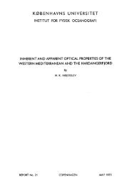
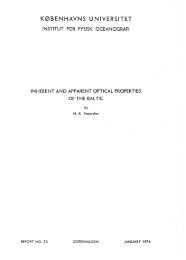
618o 2 Tox 2 ˆ T xx ;o 2 Toxoy ˆ T xz;o 2 Toy 2 ˆ T yy;o 2 Toyoz ˆ T yz2 Ground data collectiono 2 Toz 2 ˆ T zz;o 2 Toxoy ˆ T xy;Ground data may be used for two purposes. Onepurpose is the use of the data in combination withsatellite data. Another is the use of the data for thecalibration of the satellite data, i.e. the assessment of theresult of downward continued values or the detection ofpossible systematic errors in the space data. It is thelatter application which we will describe here.The gravity data set used in the present study wasmade available to the authors by R Forsberg (pers.comm). This data set includes 14,177 point free-airgravity anomalies in the area bounded by(56 / 68 ; 126 k 106 ).The distribution of the data is shown in Fig. 1. As itis seen from Fig. 1, the distribution of the data is verydense except in the area close to the meridian of)124 o and in the regions of several lakes. The statistics ofthe point gravity values are shown in Table 1. In Fig. 2the corresponding free-air gravity ®eld after removal ofthe OSU91A (Rapp and Pavlis, 1990) contribution isshown. From Fig. 2, as well as from the statistics ofTable 1, it is clear that the reduced free-air gravityanomaly ®eld is very smooth, especially in the centre ofthe test area.Omitting the data west of the meridian of )124 o , thefree-air gravity anomalies (after the removal of the-126-121-116-111-10665 6562 6259 5956 56-121-116Fig. 1. Distribution of point gravity data-111Table 1. Statistics of the free-air gravity anomalies in Canada(mGal)No. Mean SD Min MaxOriginal 14,177 )10.77 22.42 )81.10 133.00Original ) 14,177 0.95 12.68 )159.06 148.10OSU91AOriginal )OSU91A a 13,339 1.21 10.89 )42.80 73.05a After omitting the data to the west of the meridian of )124 o wherethe data coverage is poor.OSU91A contribution) covering the area (56 / 68 ; 124 k 106 ), in future called area A, wereused for the creation of simulated space data sets asdescribed in Sect. 3.3 Creation of simulated space data in the test area atdi€erent altitudesThe LSC method as implemented in the programGEOCOL (Tscherning 1995) was used to predictsatellite data from ground data at di€erent altitudes.This is done by multiplying covariances between theground and the space data with weights obtained bysolving a system of equations with a dimension equal tothe number of ground data used. If data are clustered,singularities may occur in the case of points havingalmost identical coordinates. In order to avoid thisproblem a new data set was created by selecting dataclosest to the nodes of a 3¢ ´ 3¢ grid. The equidistance ofthis grid corresponds to the mean distance between theoriginal data.The covariances of the ground data are estimated byforming products between all data and grouping thedata in bins according to the distance. In order to reducethis task, data point values were selected closest to thenodes of a 10¢ ´ 10¢ grid. In this way the empirical covariancefunction was computed from 6324 point values.The computed empirical covariance function has a correlationlength equal to about 6.5¢. The empirical covariancefunction was ®tted with an analytic expression(model) using the program COVFIT (Knudsen 1987).Using the model parameters the auto- and cross-covariancefunction of any other kind of quantities relatedto the gravity ®eld can be analytically computed, at anyaltitude. The empirical and the estimated analytical covariancefunctions of free-air gravity anomalies areshown in Fig. 3. The analytically derived values ofstandard deviations for various quantities related to thegravity ®eld at three di€erent altitudes are shown inTable 2.The correlation length of the cross-covariance functionsbetween gravity anomalies and second-order derivativesis considerably larger than the correspondingone of the auto-covariance function of gravity anomaliesat ground level. Moreover, this correlation length increaseswith altitude. In Fig. 4 the cross-covariancefunction between gravity anomalies and T zz is shown for

619-126-121-116-111-10665 65Above 140130 - 140120 - 130110 - 120100 - 11090 - 10080 - 9070 - 8060 - 7050 - 6040 - 5030 - 4020 - 3010 - 200 - 10-10 - 0-20 - -10-30 - -20-40 - -30-50 - -40-60 - -50-70 - -60-80 - -70-90 - -80-100 - -90-110 - -100-120 - -110-130 - -120-140 - -130-150 - -140-160 - -150Below -16062 6259 5956 56-121-116-111Fig. 2. The free-air gravity anomalies afterremoval of OSU91A contribution100.00.0375Covariance (mGal )262.525.0-12.5-50.00123Spherical distance (degree)Fig. 3. Covariance function of the free-air gravity anomalies reducedto OSU91A in Canada (data set A). Dashed line Empirical; solid lineanalyticalTable 2. Analytically derived standard deviations of gravity and ofthree di€erent types of second-order derivatives (for four di€erentaltitudes related to area A)Altitude(km)Gravity(mGal)T zz(EU)2*T xy(EU)T xx(EU)0 10.027 21.005 14.849 12.849200 0.200 0.017 0.012 0.010300 0.104 0.007 0.004 0.004400 0.062 0.003 0.003 0.0001three di€erent altitudes. Due to this correlation length,for the prediction of second-order derivatives in a testarea, gravity anomalies in a considerably larger area4Covariance (mGal )20.02500.01250-0.01250300 km400 km200 km1.25 2.50 3.75Spherical distance (degree)5.00Fig. 4. Cross-covariance function between free-air gravity anomaliesat ground level and Tzz at three di€erent altitudes (200, 300 and400 km)should be taken into account. For this reason, and inorder to reduce the number of input data in the collocationexperiments, a 30¢ ´ 30¢ data set of gravityanomalies was computed by averaging the point values.This data set was used as input in the LSC upwardcontinuation experiments for the computation of gravitygradients at three di€erent satellite altitudes: 200, 300and 400 km. Using LSC we computed T zz , T xx , T yy , T xz ,T yz and T xy on a 15 ´ 15 ft. grid in the area bounded by(59:5 / 64:5 ; 117:5 k 112:5 ).The equidistance of the grid was chosen to agree withthe expected resolution of the satellite gravity gradiometermeasurements. In this way, 3 ´ 6 new ®les werecreated with the simulated gradients (21 ´ 21 values per®le) at the three di€erent satellite altitudes. Simultaneously,the prediction (upward continuation) error was

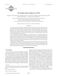
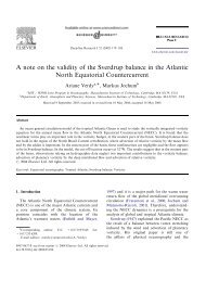
620computed. In the following this data set will be calleddata set A.Slightly better results in terms of the signal-to-noiseratio were obtained using a ``more local'' covariancefunction, i.e. a covariance function computed using onlythe data included in the point data selection area(59:5 / 64:5 ; 117:5 k 112:5 ). Thisinner area, in future called area B, is smoother than theentire area, having a variance of the gravity anomaliesequal to 52 mGal 2 (see Fig. 5). The standard deviationsfor various quantities according to this ``local'' covariancefunction are given in Table 3. In future on this dataset will be called data set B.The real satellite measurements are actually high- andlow-pass ®ltered values along track. This means thatspectral features above and below a certain frequencyare not included in their spectrum. In order to simulatesuch measurements we have to ®lter out the high- andthe low-frequency information. One way to do the ®rst isto substitute the point values by mean values along trackwith the same sampling as the real measurements. The®ltering of the lower frequencies has been simulated bysubtracting a high-order ®eld (OSU91A). If the calculationsare to be carried out for a speci®c instrument, theappropriate ®lter characteristics should obviously beused.With the following experiment we tried to investigatewhether the high-order frequencies would cause aproblem, by comparing second-order derivatives predicted:(a) as point values at a certain height and (b) asmean values along track with a certain sampling, at thesame height (computed by numerical integration).Covariance (mGal )26040200For this reason we predicted again T zz at 200 kmaltitude, in the previously mentioned 15¢ ´ 15¢ grid, asmean values along track with a data sampling correspondingto 4 s (15 arc min). Track azimuth equal to 0°was adopted in this case in order to simplify calculations.The comparison between the point and mean T zzshowed di€erences up to 0.0001 EU. These di€erencesare considered as negligible, so that in the experimentsconcerning the recovery of the systematic errors we decidedto use the ®les with the second-order derivativespredicted as point values. It should be noted that thismay not be a valid procedure in areas with a morevarying gravity ®eld.In order to study the e€ect of the resolution of thesurface data in the upward continuation procedure, weperformed four numerical experiments according to thefollowing scheme: we used point data in a2 2 ; 3 3 ; 4 4 and 5 5 area surroundedeach time by mean 30¢ ´ 30¢ data up to theouter bounds of the test ®eld. In Fig. 6 the variation ofthe prediction error for T zz along the meridian of 115°by increasing the point data collection area is shown.The Poisson integral implemented in algorithms takingadvantage of the FFT (Tscherning et al., 1994) wasalso used in order to create simulated gravity gradientdata. For this reason, the gravity anomaly ®eld was upward-continuedto 200, 300 and 400 km altitude andsubsequently these values were transformed to secondorderderivative values at the corresponding altitudes. InFig. 7 the free-air gravity anomaly ®eld at 200 km altitudeis presented, while in Fig. 8 the corresponding T zz®eld at 200 km is shown. From Fig. 7 it is seen that thefree-air gravity ®eld is very smooth at 200 km altitudeand from Fig. 8 it is evident that the T zz ®eld is stronglycorrelated with the free-air gravity ®eld. Finally, in Fig. 9the T zz component at 200 km altitude computed by LSCis presented. The computed T zz using FFT agree with thecorresponding T zz from LSC within three times the estimatederror of upward continuation calculated by LSC.4 Simulations of the recovery of systematic errors anderrors of the recovered quantities-2000.250.50 0.75 1.00Spherical distance (degree)1.251.50With LSC it is possible to study the recovery ofsystematic errors without using ``data''. The errorFig. 5. Covariance function of the free-air gravity anomalies reducedto OSU91A in Canada (data set B). Dashed line Empirical; solid lineanalyticalTable 3. Analytically derived standard deviations of gravity and ofthree di€erent types of second-order derivatives for four di€erentaltitudes (related to area B)Altitude(km)Gravity(mGal)T zz(EU)2*T xy(EU)T xx(EU)0 7.416 2.688 1.634 1.897200 0.523 0.053 0.032 0.037300 0.233 0.018 0.011 0.013400 0.126 0.008 0.004 0.005Collocation error (EU)0.010000.008750.007500.006250.0050059.560.04° x 4°3° x 3°5° x 5°60.5 61.0Latitude (degree)2° x 2°61.562.0Fig. 6. Variation of the error of prediction of Tzz at 200 km altitudealong the 115 ° meridian by increasing the point data collection area

621-126-121-116-111-10665 6562 62Above 0.70.6 - 0.70.5 - 0.60.4 - 0.50.3 - 0.40.2 - 0.30.1 - 0.20 - 0.1-0.1 - 0-0.2 - -0.1-0.3 - -0.2-0.4 - -0.3-0.5 - -0.4Below -0.559 5956 56-121-116-111Fig. 7. Free-air gravity anomalies minusOSU91A at 200 km altitude. (mGal)-126-121-116-111-106Above 0.0750.070 - 0.0750.065 - 0.0700.060 - 0.0650.055 - 0.0600.050 - 0.0550.045 - 0.0500.040 - 0.0450.035 - 0.0400.030 - 0.0350.025 - 0.0300.020 - 0.0250.015 - 0.0200.010 - 0.0150.005 - 0.0100 - 0.005-0.005 - 0-0.010 - -0.005-0.015 - -0.010-0.020 - -0.015-0.025 - -0.020-0.030 - -0.025-0.035 - -0.030-0.040 - -0.035Below -0.04065 6562 6259 5956 56-121-116-111Fig. 8. Tzz minus OSU91A at 200 kmaltitude computed by FFT (EU)estimates obtained from LSC are calculated solely fromthe covariances. However, we wanted to test theconsistency between the error estimates and di€erencesobtained using simulated data. Therefore new simulateddata sets were produced, adding biases and tilts to thepreviously described simulated gravity gradients. Thesesystematic errors were added in such a way that datalying on the same ``track'' (e.g. data with the same

622-126-121-116-111-10665 6562 62Above 0-0.01 - 0-0.01 - -0.01-0.02 - -0.01-0.02 - -0.02-0.03 - -0.02-0.03 - -0.03Below -0.0359 5956 56-121-116-111Fig. 9. Tzz ) OSU91A at 200 km altitudecomputed by LSC (EU)longitude) present the same bias and the same tilt. Theexperiments started assuming that the gradients werea€ected only by bias. However, in actual experiment onehas to assume simultaneously bias and tilt, here we weretrying to illustrate the problem step by step. In apreliminary experiment, bias was added to the T zz valuesfrom data set B at 200 km. The biased T zz values wereused to predict ground surface point data and simultaneouslyto estimate the bias parameters together withthe error of the estimation.The bias parameters in this case were 21 di€erentvalues (one per each track) with a priori known statistics(mean value and standard deviation equal to 0 and to0.03 EU, respectively). However, this standard deviationis about two times larger than the standard deviation ofe.g. T zz at 200 km altitude (see Table 2); it should bementioned that the values of Table 2 are reduced toOSU91A. The corresponding standard deviation of theunreduced quantities reaches 0.05879 EU, which isabout two times larger than the standard deviation ofthe bias parameters. With this level of systematic errorswe have values which are neither too small nor too large,when used to illustrate the results by examples. Thecomparison of the estimated with the original bias parametersshowed that the estimated quantities agreedwith the original ones within the error of estimation (seeTable 4).Since the collocation error estimates depends stronglyon the choice of the covariance function we tried tostudy the e€ect of the accuracy adopted for the data onthe results of the parameters' estimation. For this reasonthe previously described experiment was repeated assumingdata accuracies equal to 0.01 and 0.0005 EU.Table 4. Original and estimated bias parameters and the error ofestimation. The 21 original bias parameters have an a priori meanvalue and SD equal to 0 and 0.03 EU, respectively. Accuracy of theT zz values (collocation estimates) is equal to 0.005 EUOriginal biasparametersEstimatedbiasparametersError ofestimation1 )0.040 )0.054061 0.0056252 0.004 )0.009495 0.0056103 )0.038 0.050961 0.0055984 0.004 )0.008407 0.0055895 0.005 )0.006811 0.0055836 )0.069 )0.080197 0.0055787 0.036 0.015476 0.0055758 0.043 0.033178 0.0055729 0.047 0.037921 0.00557110 0.001 )0.007322 0.00557011 )0.041 )0.048520 0.00557012 0.015 0.008275 0.00557013 )0.031 )0.036945 0.00557114 0.002 )0.003139 0.00557215 0.023 0.018646 0.00557516 )0.026 )0.029578 0.00557817 )0.013 )0.015828 0.00558318 )0.052 )0.054090 0.00558919 0.007 0.005600 0.00559820 )0.023 )0.023749 0.00561021 )0.043 )0.043144 0.005625The statistics of the comparison between the originalbias parameters and the corresponding estimated aresummarized in Table 5, column 1.From Table 5 it is shown that 84.5% of the standarddeviation of the original bias has been recovered in the

623Table 5. Statistics of the differencesbetween original andestimated bias parameters forthree di€erent data accuracies(21 bias parameters). Meanerror of the estimation is shownin parenthesisData accuracyInput data (EU)T zzT zz + gravity anomaliesMean SD Mean SD0.01 0.008260 0.004657(0.0060)0.005 0.007998 0.004661(0.0059)0.0005 0.007341 0.004495(0.0056)0.000357 0.003861(0.00433)0.000313 0.003880(0.00381)0.001425 0.003966(0.00336)simple case where no crossing tracks have been used.However, there is a bias of about 0.008 EU whichshould not be ignored. This bias is due to the fact thatLSC utilizes norm-minimization to ®x the so-called nullspace. The result is a bias signi®cantly di€erent fromzero.In theory this situation could be signi®cantly improvedby combining ground level data (e.g. gravityanomalies) with the satellite second-order derivatives(null space). This was veri®ed in the next experimentswhere a set of point gravity anomalies with a resolutionof 10 ft was added to the previous T zz data set (seeTable 5, column 2). The experiment was performedagain for three di€erent accuracy values for the T zz data,while for the gravity data the value of 1 mGal wasadopted for the three cases.The lower accuracy for data accuracy equal to 0.0005is an e€ect caused by numerical instabilities of the normalequations used to compute the values. The noisevariance is in LSC added to the diagonal elements of thenormal equations, so a high noise stabilizes the solutionprocess. It therefore does not indicate that better resultscan not be obtained using other numerical procedures.The case of using crossing ground tracks (not``crossing'' at satellite altitude) is more interesting sincethe accuracy of the estimation of the bias parameters wassigni®cantly improved. In the following experiments,seven tracks in the direction East were to West wereadded to the previously described T zz data set consistingof 21 tracks in the direction from South to North, so thatthe new data set simulated crossing satellite tracks. Inthis case we have 28 bias parameters chosen also to havemean value equal to 0 and SD equal to 0.03 EU. Figure10 shows the T zz ®eld biased in this way. From this®gure it is evident that a bias with SD equal to 0.03 EUcauses a very strong distortion of the T zz ®eld. The resultsof the bias estimation (without the combination ofdata at ground level) in terms of the mean value and SDof the di€erences (original)estimated parameters) aresummarized in Table 6, column 1.However, the uncertainty in the mean is almost thesame as in the case of Table 5 (column 1) but there theSD has been considerably decreased.When surface gravity anomalies are combined withthe T zz data set there is a signi®cant improvement in themean uncertainty, as it is shown in Table 6, column 2. Inaddition, the increase in the corresponding SD after thecombination of T zz with gravity data is due to the lack ofAbove 0.060.05 - 0.060.04 - 0.050.03 - 0.040.02 - 0.030.01 - 0.020 - 0.01-0.01 - 0-0.02 - -0.01-0.03 - -0.02-0.04 - -0.03-0.05 - -0.04-0.06 - -0.05-0.07 - -0.06-0.08 - -0.07-0.09 - -0.08Below -0.0963626160-117 -116 -115 -114 -113-116 -115 -114Fig. 10. Tzz ) OSU91A at 200 km altitude arti®cially biased (EU)the stabilizing e€ect. Nevertheless, the results of Table 6are signi®cantly better than those of Table 5, at least interms of standard deviation of the di€erences betweenobserved and estimated bias parameters.Another sequence of experiments was carried outwhere the bias parameters from T zz (data set B) at altitudesof 300 and 400 km were estimated. The experimentswere performed for the cases of (a) crossing tracks(28 parameters) and (b) the combination of crossingtracks with surface gravity anomalies. In these experimentsthe a priori standard deviation of the bias parametersin 300 km altitude was set equal to 0.01 EU andfor 400 km 0.005 EU. For the T zz data an accuracy equalto 0.002 and 0.001 EU was adopted for 300 and 400 km,63626160

624Table 6. Statistics of the comparisonof the estimated biaswith the original in the case ofcrossing tracks. Number ofparameters is 28 with meanvalue 0 and SD 0.03 EU. Meanerror of the estimation is shownin parenthesisData accuracyInput data (EU)T zzT zz + gravity anomaliesMean SD Mean SD0.01 0.007403 0.000369(0.00485)0.005 0.006982 0.000182(0.00412)0.0005 0.007188 0.000024(0.00332)0.000105 0.000794(0.00393))0.000138 0.000371(0.00342)0.001478 0.000026(0.00298)Table 7. Statistics of the differences(EU) between originaland estimated bias parametersfrom crossing tracks of T zz at300 and 400 km, respectively.Mean error of the collocationestimation is given in parenthesisHeight (km)Input data (EU)T zzT zz + gravity anomaliesMean SD Mean SD300 0.005320 0.000097(0.0001942)400 0.003697 0.000051(0.001071)0.002903 0.000192(0.0001729)0.002960 0.000086(0.001025)respectively. These values are the collocation error estimatesof the prediction of T zz from gravity anomalies.The results of these experiments are shown in Table 7.In order to study the possibility of recovering the biasparameters in the case of a lower signal-to-noise ratio,we have use biased T zz from the data set A in order toestimate the bias parameters. In the experiment the apriori standard deviation of the bias parameters wasequal to 0.03 EU and the bias was estimated from (a)T zz (crossing tracks, 28 parameters) only and (b) fromcombination of T zz (crossing tracks) with surface gravityanomalies. The results from these experiments aresummarized in Table 8.Comparing the results of Table 8 (column 1) with thecorresponding results of Table 6 (column 2, row 2), wesee that in the case of data set A these are slightly betterthan the corresponding from data set B. Comparing theresults of Table 8, column 2, with the correspondingresults of Table 6 (column 2, row 2), we see that the T zzfrom data set B gives a better mean value of di€erences,but T zz from A gives better standard deviation, so thatfrom the results of the last experiments it is not possibleto draw a conclusion.In order to study the possibility of estimating a verysmall bias, e.g. of the order of 2±3% of the standarddeviation of the corresponding data in the correspondingaltitude, we performed experiments using T zz fromdata set A and bias with an a priori SD equal to0.0005 EU. The results from these experiments areshown in Table 9.From Table 9 it is also evident that a very small biascan be detected especially in the case of combiningsurface gravity anomalies with the second-order derivativesat satellite altitude.Finally, the T xz values from data set B at 200 kmhave been used in order to estimate the bias parameters.The results of this estimation are shown inTable 10.Table 9. Statistics of the di€erences (EU) between original andestimated bias parameters from T zz (data set A) at 200 km crossingtracks (28 parameters) and from a combination of T zz with surfacegravity anomalies. The a priori standard deviation of the biasparameters was equal to 0.0005 EU. For T zz data an accuracy equalto 0.005 EU was adopted. Mean error of the collocation estimationis given in parenthesisT zzT zz + gravity anomaliesMean 0.005045 0.000039SD 0.000043 (0.003619) 0.000056 (0.002511)Table 8. Statistics of the di€erences (EU) between original andestimated bias parameters from T zz (data set A) at 200 km crossingtracks (28 parameters) and from a combination of T zz with surfacegravity anomalies. The a priori standard deviation of the biasparameters was equal to 0.03 EU. For T zz data an accuracy equal to0.005 EU was adopted. Mean error of the collocation estimation isgiven in parenthesisTable 10. Statistics of the di€erences (EU) (original ± estimated)bias parameters from T xz (data set B) at 200 km crossing tracks (28parameters) and from a combination of T xz with surface gravityanomalies. The a priori standard deviation of the bias parameterswas equal to 0.03 EU. For T zz data an accuracy equal to 0.003 EUwas adopted. Mean error of the collocation estimation is given inparenthesisT zzT zz + gravity anomaliesT xzT xz + gravity anomaliesMean 0.005363 )0.000857SD 0.000138 (0.0004118) 0.000269 (0.003011)Mean )0.007924 )0.007628SD 0.000125 (0.002466) 0.000186 (0.002451)

Table 11. Statistics of the di€erences between original and estimated bias and tilt parameters from T zz (data set B) at 200 km (28 parametersfor bias and 28 for tilt), alone or in combination with surface gravity data. The a priori standard deviation of the bias parameters was equalto 0.003 EU and that of the tilt equal to 0.003 EU/100 km. For the T zz data an accuracy equal to 0.005 EU was adopted. Mean error of thecollocation estimation is given in parenthesis625Bias (EU)Tilt (EU/100 km)Mean SD Mean SDCrossing tracks )0.007050 0.005778 (0.008205) )0.000014 0.000397 (0.000652)Crossing tracks + gravity )0.000178 0.005679 (0.006630) 0.000014 0.000394 (0.000559)anomaliesConsidering the results of Table 10, we see that thebias remains almost the same even after the combinationof surface gravity anomalies. Concerning the standarddeviation of the di€erences (observed ) predicted), thesituation is very similar to the corresponding one whenusing the T zz values for the bias estimation.The experiments for the estimation of systematic errorswere completed by investigating the case where thedata are a€ected simultaneously by bias and tilt, sincethis is the realistic situation. For this reason tilt wasarti®cially added to the already biased predicted secondorderderivatives, used in the previous experiments forthe recovery of the bias parameters. The tilt addedpresents a mean value equal to 0 EU and a SD equal to0.003 EU/100 km. This value was selected based on theobservation that the total length of the simulated tracksin the North±South direction is about 555 km, so the SDof the tilt of a track from North to South is about 0.017EU, i.e. equal to the SD of the T zz values (data set A) at200 km altitude. The results summarized in Table 11concern the bias and tilt estimation in the case of (a) T zzcrossing tracks, and (b) T zz crossing tracks combinedwith surface gravity anomalies.From the results of Table 11 we see that the standarddeviation of the di€erences between original and estimatedbias and tilt agree with the corresponding meanerror estimate from collocation. As in the earlier results,this is only showing that the actual software implementation(GEOCOL) works correctly.5 ConclusionThe described simulations showed that the recovery ofbias parameters from second-order derivative SGG``measurements'' is possible with an accuracy down to50% of the random data noise. The use of crossingtracks helps to improve the bias estimation.The mean value of the di€erences (original ) estimatedbias parameters) obtained from simulated data isrelatively large compared to the standard deviation ofthe corresponding second-order derivative component atthe corresponding height. This mean value almost vanisheswhen gravity data at ground level are combinedwith the second-order derivative data set. This shows theusefulness of combining space data with ground data.In the case of simultaneous estimation of bias and tiltparameters from T zz ``measurements'', the collocationerror estimates are double the error estimates obtainedwhen the observations are only supposed to be contaminatedby a bias noise. However, this error is still atthe level of the supposed random data noise. This veri-®es that such errors can be consistently removed.Acknowledgements. Thanks are due to R. Forsberg (NationalSurvey & Cadastre, Denmark) for providing gravity data and toR.H. Rapp (Columbus, Ohio) for the OSU91A model. This paperhas been carried out in the framework of a project supported byESA/ESTEC contract JP/95-4-137/MS/NR.ReferencesKnudsen P (1987) Estimation and modelling of the local empiricalcovariance function using gravity and satellite altimeter data.Bull Geod 61: 145±160Moritz H (1980) Advanced physical geodesy. H. Wichmann,KarlsruheRapp RH, Pavlis NK (1990) The development of geopotentialcoecient models to spherical harmonic degree 360. J GeophysRes 95: 21885±21911Schwarz KP, Sideris MG, Forsberg R (1990) The use of FFTtechniques in physical geodesy. Geophys J Int 100: 485±514Tscherning CC (1995) GEOCOL ± a FORTRAN program forgravity ®eld approximation by collocation, 11th edn. Technicalnote, Geophysical Institute, University of CopenhagenTscherning CC, Knudsen P, Forsberg R (1994) Description of theGRAVSOFT package, 4th edn. Technical report, GeophysicalInstitute, University of Copenhagen