Chapter 06.05 Adequacy of Models for Regression
Chapter 06.05 Adequacy of Models for Regression
Chapter 06.05 Adequacy of Models for Regression

You also want an ePaper? Increase the reach of your titles
YUMPU automatically turns print PDFs into web optimized ePapers that Google loves.
<strong>06.05</strong>.2 <strong>Chapter</strong> <strong>06.05</strong>Figure 1 Plot <strong>of</strong> coefficient <strong>of</strong> thermal expansion vs. temperature data points and regressionline.2. Calculate the standard error <strong>of</strong> estimate.The standard error <strong>of</strong> estimate is defined asSrsα/ T= n − 2whereSr=n∑i=1(αi− a0 − a1Ti)2Table 2 Residuals <strong>for</strong> data.Ti-340-260-180-100-2060αi2.453.584.525.285.866.36α −a + 0a1Tiia − 0a1Ti2.73573.51144.28715.06295.83866.6143-0.285710.0685710.232860.217140.021429-0.25429
<strong>Adequacy</strong> <strong>of</strong> <strong>Regression</strong> Model <strong>06.05</strong>.3Table 2 shows the residuals <strong>of</strong> the data to calculate the sum <strong>of</strong> the square <strong>of</strong> residuals as2222= ( −0.28571)+ (0.068571) + (0.23286) + (0.21714)S r+ (0.021429)= 0.25283The standard error <strong>of</strong> estimateSrsα/ T= n − 22+ ( −0.25429)0.25283=6 − 2= 0.25141The units <strong>of</strong> s α / Tare same as the units <strong>of</strong> α . How is the value <strong>of</strong> the standard error <strong>of</strong>estimate interpreted? We may say that on average the difference between the observed andpredicted values is 0.25141μin/in/ F . Also, we can look at the value as follows. About 95%<strong>of</strong> the observed α values are between ± 2s α / T<strong>of</strong> the predicted value (see Figure 2). Thiswould lead us to believe that the value <strong>of</strong> α in the example is expected to be accurate within± = ± 2 × 0. 25141= ± 0.50282 μin/in/ F .2s α / T2Figure 2 Plotting the linear regression line and showing the regression standard error.
<strong>06.05</strong>.4 <strong>Chapter</strong> <strong>06.05</strong>One can also look at this criterion as finding if 95% <strong>of</strong> the scaled residuals <strong>for</strong> the model arein the domain [-2,2], that isαi− a0− a1TiScaled residual =sα/ TFor the example,s α / T= 0.25141Table 4 Residuals and scaled residuals <strong>for</strong> data.Tiαiα − ia 0a1TiScaled Residuals-340-260-180-100-20602.453.584.525.285.866.36-0.285710.0685710.232860.217140.021429-0.25429-1.13640.272750.926220.863690.085235-1.0115and the scaled residuals are calculated in Table 4. All the scaled residuals are in the [-2,2]domain.3. Calculate the coefficient <strong>of</strong> determination.Denoted by r 2 , the coefficient <strong>of</strong> determination is another criterion to use <strong>for</strong> checking theadequacy <strong>of</strong> the model.To answer the above questions, let us start from the examination <strong>of</strong> some measures <strong>of</strong>discrepancies between the whole data and some key central tendency. Look at the twoequations given below.whereSrS t===n∑i=1n( α − ˆ α )αii=α = 1 nFor the example datai∑( αi− a0− a1Ti)i22i=1n2∑( αi−α)(2)i=1n∑6∑αi= 1α = i 62 .45 + 3.58 + 4.52 + 5.28 + 5.86 + 6.36=6= 4.6750 μin/in/ F(1)
<strong>Adequacy</strong> <strong>of</strong> <strong>Regression</strong> Model <strong>06.05</strong>.5S t=n∑( αi−α)2i=122222( −2.2250)+ ( −1.0950)+ ( −0.15500)+ (0.60500) + (1.1850) +== 10.783(1.6850)2Table 5 Difference between observed and average value.Tiαiα i−α-340 2.45 -2.2250-260 3.58 -1.0950-180 4.52 -0.15500-100 5.28 0.60500-20 5.86 1.185060 6.36 1.6850where Sris the sum <strong>of</strong> the square <strong>of</strong> the residuals (residual is the difference between theobserved value and the predicted value), and Stis the sum <strong>of</strong> the square <strong>of</strong> the differencebetween the observed value and the average value.What inferences can we make about the two equations? Equation (2) measures thediscrepancy between the data and the mean. Recall that the mean <strong>of</strong> the data is a measure <strong>of</strong>a single point that measures the central tendency <strong>of</strong> the whole data. Equation (2) contrastswith Equation (1) as Equation (1) measures the discrepancy between the vertical distance <strong>of</strong>the point from the regression line (another measure <strong>of</strong> central tendency). This line obtainedby the least squares method gives the best estimate <strong>of</strong> a line with least sum <strong>of</strong> deviation. Sras calculated quantifies the spread around the regression line.The objective <strong>of</strong> least squares method is to obtain a compact equation that bestdescribes all the data points. The mean can also be used to describe all the data points. Themagnitude <strong>of</strong> the sum <strong>of</strong> squares <strong>of</strong> deviation from the mean or from the least squares line isthere<strong>for</strong>e a good indicator <strong>of</strong> how well the mean or least squares characterizes thewhole data. We can liken the sum <strong>of</strong> squares deviation around the mean, Stas the error orvariability in y without considering the regression variable x , while Sr, the sum <strong>of</strong> squaresdeviation around the least square regression line is error or variability in y remaining afterthe dependent variable x has been considered.The difference between these two parameters measures the error due to describing orcharacterizing the data in one <strong>for</strong>m instead <strong>of</strong> the other. A relative comparison <strong>of</strong> thisdifference ( St − S r), with the sum <strong>of</strong> squares deviation associated with the mean Stdescribes2a quantity called coefficient <strong>of</strong> determination, r2 St− Srr =(5)St10.783− 0.25283=10.783= 0.97655
<strong>06.05</strong>.6 <strong>Chapter</strong> <strong>06.05</strong>Based on the value obtained above, we can claim that 97.7% <strong>of</strong> the original uncertainty in thevalue <strong>of</strong> α can be explained by the straight-line regression model <strong>of</strong>α ( T ) = 6.0325 + 0. 0096964T .Going back to the definition <strong>of</strong> the coefficient <strong>of</strong> determination, one can see that Stis thevariation without any relationship <strong>of</strong> y vs. x , while Sris the variation with the straight-linerelationship.2The limits <strong>of</strong> the values <strong>of</strong> r are between 0 and 1. What do these limiting values <strong>of</strong>2r mean? If r 2 = 0 , then St= Sr, which means that regressing the data to a straight linedoes nothing to explain the data any further. If r 2 = 1, then Sr= 0 , which means that thestraight line is passing through all the data points and is a perfect fit.Caution in the use <strong>of</strong>2r2a) The coefficient <strong>of</strong> determination, r can be made larger (assumes no collinear points)by adding more terms to the model. For instance, n −1terms in a regression equation<strong>for</strong> which n data points are used will give an r 2 value <strong>of</strong> 1 if there are no collinearpoints.b) The magnitude <strong>of</strong> r 2 also depends on the range <strong>of</strong> variability <strong>of</strong> the regressor (x)2variable. Increase in the spread <strong>of</strong> x increases r while a decrease in the spread <strong>of</strong> xdecreases r 2 .2c) Large regression slope will also yield artificially high r .d) The coefficient <strong>of</strong> determination, r 2 does not measure the appropriateness <strong>of</strong> the2linear model. r may be large <strong>for</strong> nonlinearly related x and y values.2e) Large coefficient <strong>of</strong> determination r value does not necessarily imply the regressionwill predict accurately.2f) The coefficient <strong>of</strong> determination , r does not measure the magnitude <strong>of</strong> the regressionslope.g) These statements above imply that one should not choose a regression model solely2based on consideration <strong>of</strong> r .4. Find if the model meets the assumptions <strong>of</strong> random errors.These assumptions include that the residuals are negative as well as positive to give a mean<strong>of</strong> zero, the variation <strong>of</strong> the residuals as a function <strong>of</strong> the independent variable is random, theresiduals follow a normal distribution, and that there is no auto correlation between the datapoints.To illustrate this better, we have an extended data set <strong>for</strong> the example that we took.Instead <strong>of</strong> 6 data points, this set has 22 data points (Table 6). Drawing conclusions fromsmall or large data sets <strong>for</strong> checking assumption <strong>of</strong> random error is not recommended.
<strong>Adequacy</strong> <strong>of</strong> <strong>Regression</strong> Model <strong>06.05</strong>.7Table 6 Instantaneous thermal expansion coefficient as a function <strong>of</strong> temperature.TemperatureInstantaneousThermal Expansion° Fμin/in/° F80 6.4760 6.3640 6.2420 6.120 6.00-20 5.86-40 5.72-60 5.58-80 5.43-100 5.28-120 5.09-140 4.91-160 4.72-180 4.52-200 4.30-220 4.08-240 3.83-260 3.58-280 3.33-300 3.07-320 2.76-340 2.45
<strong>06.05</strong>.8 <strong>Chapter</strong> <strong>06.05</strong>Figure 3 Plot <strong>of</strong> thermal expansion coefficient vs. temperature data points and regression line<strong>for</strong> more data points.Regressing the data from Table 2 to the straight line regression lineα ( T ) = a0+ a1Tand following the procedure <strong>for</strong> conducting linear regression as given in <strong>Chapter</strong> 06.03, weget (Figure 3)α = 6 .0248 + 0.0093868T
<strong>Adequacy</strong> <strong>of</strong> <strong>Regression</strong> Model <strong>06.05</strong>.9Figure 4 Plot <strong>of</strong> residuals.Figure 4 shows the residuals <strong>for</strong> the example as a function <strong>of</strong> temperature. Althoughthe residuals seem to average to zero, but within a range, they do not exhibit this zero mean.For an initial value <strong>of</strong> T , the averages are below zero. For the middle values <strong>of</strong> T , theaverages are below zero, and again <strong>for</strong> the final values <strong>of</strong> T , the averages are below zero.This may be considered a violation <strong>of</strong> the model assumption.Figure 4 also shows the residuals <strong>for</strong> the example are following a nonlinear variance.This is a clear violation <strong>of</strong> the model assumption <strong>of</strong> constant variance.
<strong>06.05</strong>.10 <strong>Chapter</strong> <strong>06.05</strong>Figure 5 Histogram <strong>of</strong> residuals.Figure 5 shows the histogram <strong>of</strong> the residuals. Clearly, the histogram is not showinga normal distribution, and hence violates the model assumption <strong>of</strong> normality.To check that there is no autocorrelation between observed values, the following rule<strong>of</strong> thumb can be used. If n is the number <strong>of</strong> data points, and q is the number <strong>of</strong> times thesign <strong>of</strong> the residual changes, then if( n −1)n −1− n −1≤ q ≤ + n −1,22you most likely do not have an autocorrelation. For the example, n = 22 , then(22 −1)22 −1− 22 −1≤ q ≤ + 22 −1225.9174≤ q ≤ 15.083is not satisfied as q = 2 . So this model assumption is violated.ReferencesADEQUACY OF REGRESSION MODELSTopic <strong>Adequacy</strong> <strong>of</strong> <strong>Regression</strong> <strong>Models</strong>Summary Textbook notes <strong>of</strong> <strong>Adequacy</strong> <strong>of</strong> <strong>Regression</strong> <strong>Models</strong>Major General Engineering
<strong>Adequacy</strong> <strong>of</strong> <strong>Regression</strong> Model <strong>06.05</strong>.11Authors Autar Kaw, Egwu KaluDate May 31, 2013Web Site http://numericalmethods.eng.usf.edu