Wireless Ad Hoc and Sensor Networks

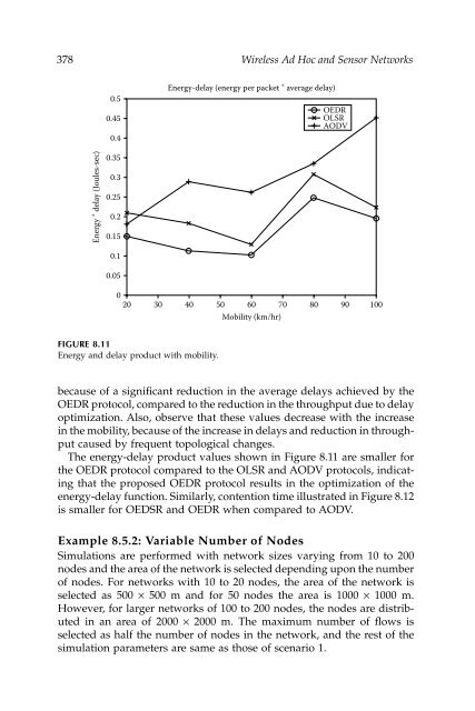
378 Wireless Ad Hoc and Sensor Networks0.50.450.4Energy-delay (energy per packet ∗ average delay)OEDROLSRAODVEnergy ∗ delay (Joules-sec)0.350.30.250.20.150.10.05020 30 40 50 60 70Mobility (km/hr)80 90 100FIGURE 8.11Energy and delay product with mobility.because of a significant reduction in the average delays achieved by theOEDR protocol, compared to the reduction in the throughput due to delayoptimization. Also, observe that these values decrease with the increasein the mobility, because of the increase in delays and reduction in throughputcaused by frequent topological changes.The energy-delay product values shown in Figure 8.11 are smaller forthe OEDR protocol compared to the OLSR and AODV protocols, indicatingthat the proposed OEDR protocol results in the optimization of theenergy-delay function. Similarly, contention time illustrated in Figure 8.12is smaller for OEDSR and OEDR when compared to AODV.Example 8.5.2: Variable Number of NodesSimulations are performed with network sizes varying from 10 to 200nodes and the area of the network is selected depending upon the numberof nodes. For networks with 10 to 20 nodes, the area of the network isselected as 500 × 500 m and for 50 nodes the area is 1000 × 1000 m.However, for larger networks of 100 to 200 nodes, the nodes are distributedin an area of 2000 × 2000 m. The maximum number of flows isselected as half the number of nodes in the network, and the rest of thesimulation parameters are same as those of scenario 1.