Wireless Ad Hoc and Sensor Networks
Wireless Ad Hoc and Sensor Networks Wireless Ad Hoc and Sensor Networks
Distributed Power Control of Wireless Cellular and Peer-to-Peer Networks 185This is a stable linear system driven by a constant bounded input η i .Applying the well-known theory of linear systems (Lewis 1999), it is easyito show that xi( ∞ ) = η . In the absence of protection margin, the SIRkierror approaches to zero as t →∞.x iREMARK 1The transmission power is subject to the constraint pmin≤ pi≤ pmaxwherep min is the minimum value needed to transmit, p max is the maximumallowed power, and p i is the transmission power of the user i. Hence, fromEquation 5.11, pi( l+ 1)can be written as pi( l+ 1) = min( pmax, ( vi( l) Ii( l) + pi( l))).The power update presented in Theorem 5.2.1 does not use any optimizationfunction. Hence, it may not render optimal transmitter powervalues though it guarantees convergence of actual SIR of each link to itstarget. Therefore, in Table 5.2, an optimal DPC is proposed.THEOREM 5.2.2 (OPTIMAL CONTROL)Given the hypothesis presented in the previous Theorem 5.2.1, for DPC, with thefeedback selected as v() l =− k x() l +η , where the feedback gains are taken asi i i i( )−1k = H S H + T H S Ji i T ∞ i i i T ∞ i(5.14)TABLE 5.2Optimal Distributed Power ControllerSIR system state equationPerformance indexSIR errorAssumptionsFeedback controllerPower updateR( l+ 1) = R( l) + v () l∞∑i=1i i ixTx+vQvi T i i i T i ix () l = R()l −γi i iTi ≥ 0, Qi> 0 all are symmetricT−1TS = J [ S − SH ( H S H + T) H S ] J + Qiii i i iTi i i iT− Tk = ( H S H + T) 1 H S Jii∞v () l =− k x () l +ηi i i ii i ip( l+ 1) = ( v ( l) I ( l) + p( l))i i i i∞iiiwherek i, γ i , andηi are design parameters
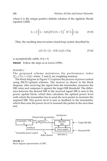
186 Wireless Ad Hoc and Sensor Networkswhere is the unique positive definite solution of the algebraic Ricattiequation (ARE)S iS J S SH H S H T H S J Q( )⎡= − +⎣⎢⎤⎦⎥ +i i T i i i i T i i i i T i i−1(5.15)Then, the resulting time-invariant closed-loop system described byx( l+ 1) = ( J − HK ) x( l)+ Hηi i i i i i i(5.16)is asymptotically stable, if = 0.PROOF Follow the steps as in Lewis (1999).η iREMARK 2The proposed scheme minimizes the performance index∞∑ i=xTx i T i i + vQv i T i i where and are weighting matrices.The block diagram in Figure 5.1 explains the process of power controlusing SSCD/optimal schemes. The receiver as shown in the blockdiagram, after receiving the signal from the transmitter, measures theSIR value and compares it against the target SIR threshold. The differencebetween the desired SIR to the received signal SIR is sent to thepower update block, which then calculates the optimal power levelwith which the transmitter has to send the next packet to maintain therequired SIR. This power level is sent as feedback to the transmitter,which then uses the power level to transmit the packet in the next timeslot.1 T i Q iInterferenceTransmitter ∗ TPCP iFeedback∗ Transmitter power controlChannel with uncertaintiesTPC commandRadio channelReceiverDPCPower updateIEEE 802.11Target SIR (dB)Measured SIRFIGURE 5.1Block diagram representation of DPC.
- Page 157 and 158: 134 Wireless Ad Hoc and Sensor Netw
- Page 159 and 160: 136 Wireless Ad Hoc and Sensor Netw
- Page 161 and 162: 138 Wireless Ad Hoc and Sensor Netw
- Page 163 and 164: 140 Wireless Ad Hoc and Sensor Netw
- Page 165 and 166: 142 Wireless Ad Hoc and Sensor Netw
- Page 167 and 168: 144 Wireless Ad Hoc and Sensor Netw
- Page 170 and 171: 4Admission Controller Design for Hi
- Page 172 and 173: Admission Controller Design for Hig
- Page 174 and 175: Admission Controller Design for Hig
- Page 176 and 177: Admission Controller Design for Hig
- Page 178 and 179: Admission Controller Design for Hig
- Page 180 and 181: Admission Controller Design for Hig
- Page 182 and 183: Admission Controller Design for Hig
- Page 184 and 185: Admission Controller Design for Hig
- Page 186 and 187: Admission Controller Design for Hig
- Page 188 and 189: Admission Controller Design for Hig
- Page 190 and 191: Admission Controller Design for Hig
- Page 192 and 193: Admission Controller Design for Hig
- Page 194 and 195: Admission Controller Design for Hig
- Page 196 and 197: Admission Controller Design for Hig
- Page 198: Admission Controller Design for Hig
- Page 201 and 202: 178 Wireless Ad Hoc and Sensor Netw
- Page 203 and 204: 180 Wireless Ad Hoc and Sensor Netw
- Page 205 and 206: 182 Wireless Ad Hoc and Sensor Netw
- Page 207: 184 Wireless Ad Hoc and Sensor Netw
- Page 211 and 212: 188 Wireless Ad Hoc and Sensor Netw
- Page 213 and 214: 190 Wireless Ad Hoc and Sensor Netw
- Page 215 and 216: 192 Wireless Ad Hoc and Sensor Netw
- Page 217 and 218: 194 Wireless Ad Hoc and Sensor Netw
- Page 219 and 220: 196 Wireless Ad Hoc and Sensor Netw
- Page 221 and 222: 198 Wireless Ad Hoc and Sensor Netw
- Page 223 and 224: 200 Wireless Ad Hoc and Sensor Netw
- Page 225 and 226: 202 Wireless Ad Hoc and Sensor Netw
- Page 227 and 228: 204 Wireless Ad Hoc and Sensor Netw
- Page 229 and 230: 206 Wireless Ad Hoc and Sensor Netw
- Page 231 and 232: 208 Wireless Ad Hoc and Sensor Netw
- Page 233 and 234: 210 Wireless Ad Hoc and Sensor Netw
- Page 235 and 236: 212 Wireless Ad Hoc and Sensor Netw
- Page 237 and 238: 214 Wireless Ad Hoc and Sensor Netw
- Page 239 and 240: 216 Wireless Ad Hoc and Sensor Netw
- Page 241 and 242: 218 Wireless Ad Hoc and Sensor Netw
- Page 243 and 244: 220 Wireless Ad Hoc and Sensor Netw
- Page 245 and 246: 222 Wireless Ad Hoc and Sensor Netw
- Page 247 and 248: 224 Wireless Ad Hoc and Sensor Netw
- Page 249 and 250: 226 Wireless Ad Hoc and Sensor Netw
- Page 251 and 252: 228 Wireless Ad Hoc and Sensor Netw
- Page 253 and 254: 230 Wireless Ad Hoc and Sensor Netw
- Page 255 and 256: 232 Wireless Ad Hoc and Sensor Netw
- Page 257 and 258: 234 Wireless Ad Hoc and Sensor Netw
186 <strong>Wireless</strong> <strong>Ad</strong> <strong>Hoc</strong> <strong>and</strong> <strong>Sensor</strong> <strong>Networks</strong>where is the unique positive definite solution of the algebraic Ricattiequation (ARE)S iS J S SH H S H T H S J Q( )⎡= − +⎣⎢⎤⎦⎥ +i i T i i i i T i i i i T i i−1(5.15)Then, the resulting time-invariant closed-loop system described byx( l+ 1) = ( J − HK ) x( l)+ Hηi i i i i i i(5.16)is asymptotically stable, if = 0.PROOF Follow the steps as in Lewis (1999).η iREMARK 2The proposed scheme minimizes the performance index∞∑ i=xTx i T i i + vQv i T i i where <strong>and</strong> are weighting matrices.The block diagram in Figure 5.1 explains the process of power controlusing SSCD/optimal schemes. The receiver as shown in the blockdiagram, after receiving the signal from the transmitter, measures theSIR value <strong>and</strong> compares it against the target SIR threshold. The differencebetween the desired SIR to the received signal SIR is sent to thepower update block, which then calculates the optimal power levelwith which the transmitter has to send the next packet to maintain therequired SIR. This power level is sent as feedback to the transmitter,which then uses the power level to transmit the packet in the next timeslot.1 T i Q iInterferenceTransmitter ∗ TPCP iFeedback∗ Transmitter power controlChannel with uncertaintiesTPC comm<strong>and</strong>Radio channelReceiverDPCPower updateIEEE 802.11Target SIR (dB)Measured SIRFIGURE 5.1Block diagram representation of DPC.


