Wireless Ad Hoc and Sensor Networks
Wireless Ad Hoc and Sensor Networks Wireless Ad Hoc and Sensor Networks
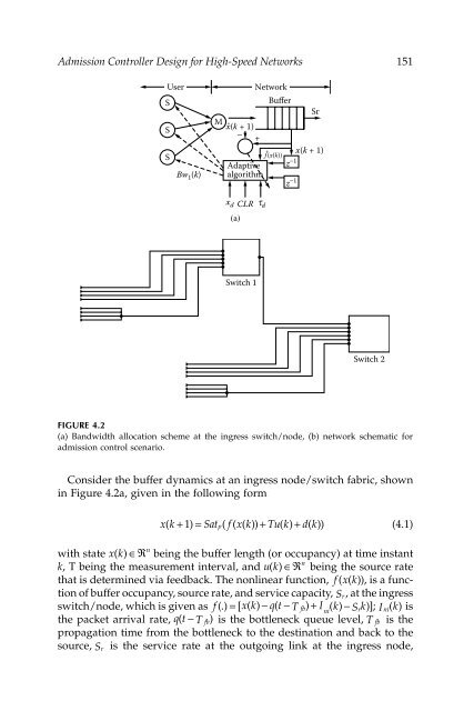
Admission Controller Design for High-Speed Networks 151UserSSSBw 1 (k)NetworkBufferSrMx(k + 1)− +x(k + 1)f (x(k))Adaptive z −1algorithmz −1x d CLR(a)t dSwitch 1Switch 2FIGURE 4.2(a) Bandwidth allocation scheme at the ingress switch/node, (b) network schematic foradmission control scenario.Consider the buffer dynamics at an ingress node/switch fabric, shownin Figure 4.2a, given in the following formxk ( + 1) = Sat( f( xk ( )) + Tuk ( ) + dk ( ))p(4.1)nwith state xk ( )∈R being the buffer length (or occupancy) at time instantnk, T being the measurement interval, and uk ( )∈R being the source ratethat is determined via feedback. The nonlinear function, f( x( k)), is a functionof buffer occupancy, source rate, and service capacity, S r , at the ingressswitch/node, which is given as f (.) = [ xk ( ) −qt ( − T fb) + I ( k) − S k ; isni r )] I ni( k)the packet arrival rate, qt ( − T fb)is the bottleneck queue level, T fb is thepropagation time from the bottleneck to the destination and back to thesource, is the service rate at the outgoing link at the ingress node,S r
152 Wireless Ad Hoc and Sensor Networksand Sat (.) is a saturation function that satisfies the following:pSat () z = 0,ifz ≤ 0,This value of T fb is obtained from the round-trip delay time (RTT−RTT min), where RTT is the round-trip delay and RTT min is the minimumpropagation time obtained from the link bandwidth. The unknown disturbancevector acting on the system at the instant k is dk ( )∈R , which isnassumed to be bounded by a known constant |( dk)|≤ d M . Here, the disturbancevector dk ( ) can be an unexpected traffic burst/load or change inavailable bandwidth owing to the presence of a network fault. Thestate xk ( ) is a positive scalar if a single-switch or single-buffer scenario isconsidered, whereas it becomes a vector when multiple network switchesor multiple buffers are involved. The first step in the proposed approachis to estimate the buffer occupancy, using an estimate of the network trafficat the switch. For the sake of convenience, we will eliminate saturationby not allowing xk ( ) to saturate.The objective here is to construct a model to identify the traffic accumulationat the switch as:xk ˆ( + 1 ) = f ˆ( xk ( )) + Tuk ( ) , (4.2)nwhere the state of the model, xk ˆ( ) ∈R , is the buffer occupancy estimateat time instant k, with the nonlinear function f ˆ( x( k))being the trafficaccumulation estimate. Define the performance criterion in terms of bufferoccupancy estimation error aswhere the packet/cell losses, for a buffer size ofp= p,if z ≥ p,= z, otherwiseek ( ) = xk ( ) −xkˆ( ), (4.3)x d, are given byck ( ) = max( 0, ek ( ))(4.4)Equation 4.3 can be expressed using Equation 4.4 and Equation 4.5 as:ek ( + 1) = f̃( xk ( )) + dk ( ), (4.5)where ek ( + 1)and xk ( + 1)denote the error in buffer occupancy and thebuffer occupancy at the instant , respectively, and the traffic flowmodeling error is given by ̃f k + 1( x ( k )) = f ( x ( k )) − f ˆ( x ( k )) . Equation 4.5 relatesthe buffer occupancy estimation error with the traffic flow modeling error.
- Page 123 and 124: 100 Wireless Ad Hoc and Sensor Netw
- Page 125 and 126: 102 Wireless Ad Hoc and Sensor Netw
- Page 127 and 128: 104 Wireless Ad Hoc and Sensor Netw
- Page 129 and 130: 106 Wireless Ad Hoc and Sensor Netw
- Page 131 and 132: 108 Wireless Ad Hoc and Sensor Netw
- Page 133 and 134: 110 Wireless Ad Hoc and Sensor Netw
- Page 135 and 136: 112 Wireless Ad Hoc and Sensor Netw
- Page 137 and 138: 114 Wireless Ad Hoc and Sensor Netw
- Page 139 and 140: 116 Wireless Ad Hoc and Sensor Netw
- Page 141 and 142: 118 Wireless Ad Hoc and Sensor Netw
- Page 143 and 144: 120 Wireless Ad Hoc and Sensor Netw
- Page 145 and 146: 122 Wireless Ad Hoc and Sensor Netw
- Page 147 and 148: 124 Wireless Ad Hoc and Sensor Netw
- Page 149 and 150: 126 Wireless Ad Hoc and Sensor Netw
- Page 151 and 152: 128 Wireless Ad Hoc and Sensor Netw
- Page 153 and 154: 130 Wireless Ad Hoc and Sensor Netw
- Page 155 and 156: 132 Wireless Ad Hoc and Sensor Netw
- Page 157 and 158: 134 Wireless Ad Hoc and Sensor Netw
- Page 159 and 160: 136 Wireless Ad Hoc and Sensor Netw
- Page 161 and 162: 138 Wireless Ad Hoc and Sensor Netw
- Page 163 and 164: 140 Wireless Ad Hoc and Sensor Netw
- Page 165 and 166: 142 Wireless Ad Hoc and Sensor Netw
- Page 167 and 168: 144 Wireless Ad Hoc and Sensor Netw
- Page 170 and 171: 4Admission Controller Design for Hi
- Page 172 and 173: Admission Controller Design for Hig
- Page 176 and 177: Admission Controller Design for Hig
- Page 178 and 179: Admission Controller Design for Hig
- Page 180 and 181: Admission Controller Design for Hig
- Page 182 and 183: Admission Controller Design for Hig
- Page 184 and 185: Admission Controller Design for Hig
- Page 186 and 187: Admission Controller Design for Hig
- Page 188 and 189: Admission Controller Design for Hig
- Page 190 and 191: Admission Controller Design for Hig
- Page 192 and 193: Admission Controller Design for Hig
- Page 194 and 195: Admission Controller Design for Hig
- Page 196 and 197: Admission Controller Design for Hig
- Page 198: Admission Controller Design for Hig
- Page 201 and 202: 178 Wireless Ad Hoc and Sensor Netw
- Page 203 and 204: 180 Wireless Ad Hoc and Sensor Netw
- Page 205 and 206: 182 Wireless Ad Hoc and Sensor Netw
- Page 207 and 208: 184 Wireless Ad Hoc and Sensor Netw
- Page 209 and 210: 186 Wireless Ad Hoc and Sensor Netw
- Page 211 and 212: 188 Wireless Ad Hoc and Sensor Netw
- Page 213 and 214: 190 Wireless Ad Hoc and Sensor Netw
- Page 215 and 216: 192 Wireless Ad Hoc and Sensor Netw
- Page 217 and 218: 194 Wireless Ad Hoc and Sensor Netw
- Page 219 and 220: 196 Wireless Ad Hoc and Sensor Netw
- Page 221 and 222: 198 Wireless Ad Hoc and Sensor Netw
- Page 223 and 224: 200 Wireless Ad Hoc and Sensor Netw
<strong>Ad</strong>mission Controller Design for High-Speed <strong>Networks</strong> 151UserSSSBw 1 (k)NetworkBufferSrMx(k + 1)− +x(k + 1)f (x(k))<strong>Ad</strong>aptive z −1algorithmz −1x d CLR(a)t dSwitch 1Switch 2FIGURE 4.2(a) B<strong>and</strong>width allocation scheme at the ingress switch/node, (b) network schematic foradmission control scenario.Consider the buffer dynamics at an ingress node/switch fabric, shownin Figure 4.2a, given in the following formxk ( + 1) = Sat( f( xk ( )) + Tuk ( ) + dk ( ))p(4.1)nwith state xk ( )∈R being the buffer length (or occupancy) at time instantnk, T being the measurement interval, <strong>and</strong> uk ( )∈R being the source ratethat is determined via feedback. The nonlinear function, f( x( k)), is a functionof buffer occupancy, source rate, <strong>and</strong> service capacity, S r , at the ingressswitch/node, which is given as f (.) = [ xk ( ) −qt ( − T fb) + I ( k) − S k ; isni r )] I ni( k)the packet arrival rate, qt ( − T fb)is the bottleneck queue level, T fb is thepropagation time from the bottleneck to the destination <strong>and</strong> back to thesource, is the service rate at the outgoing link at the ingress node,S r


