Wireless Ad Hoc and Sensor Networks

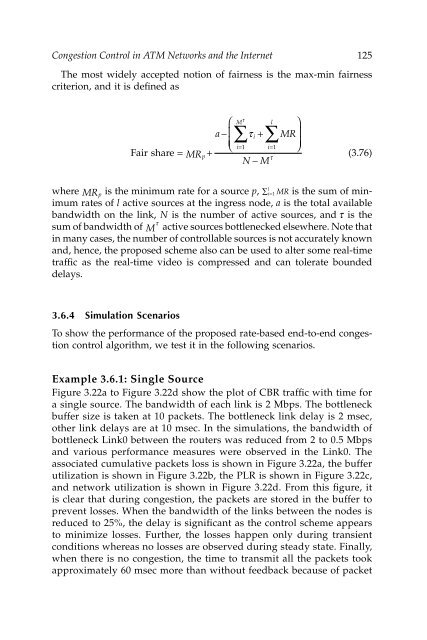
Congestion Control in ATM Networks and the Internet 125The most widely accepted notion of fairness is the max-min fairnesscriterion, and it is defined asτ⎛ M l ⎞a− ⎜ i + MR⎝⎜∑τ∑⎟i i ⎠⎟= 1 = 1Fair share = MRp+(3.76)τN−Mlwhere MRpis the minimum rate for a source p, ∑ i=1 MR is the sum of minimumrates of l active sources at the ingress node, a is the total availablebandwidth on the link, N is the number of active sources, and τ is theτsum of bandwidth of M active sources bottlenecked elsewhere. Note thatin many cases, the number of controllable sources is not accurately knownand, hence, the proposed scheme also can be used to alter some real-timetraffic as the real-time video is compressed and can tolerate boundeddelays.3.6.4 Simulation ScenariosTo show the performance of the proposed rate-based end-to-end congestioncontrol algorithm, we test it in the following scenarios.Example 3.6.1: Single SourceFigure 3.22a to Figure 3.22d show the plot of CBR traffic with time fora single source. The bandwidth of each link is 2 Mbps. The bottleneckbuffer size is taken at 10 packets. The bottleneck link delay is 2 msec,other link delays are at 10 msec. In the simulations, the bandwidth ofbottleneck Link0 between the routers was reduced from 2 to 0.5 Mbpsand various performance measures were observed in the Link0. Theassociated cumulative packets loss is shown in Figure 3.22a, the bufferutilization is shown in Figure 3.22b, the PLR is shown in Figure 3.22c,and network utilization is shown in Figure 3.22d. From this figure, itis clear that during congestion, the packets are stored in the buffer toprevent losses. When the bandwidth of the links between the nodes isreduced to 25%, the delay is significant as the control scheme appearsto minimize losses. Further, the losses happen only during transientconditions whereas no losses are observed during steady state. Finally,when there is no congestion, the time to transmit all the packets tookapproximately 60 msec more than without feedback because of packet