Wireless Ad Hoc and Sensor Networks
Wireless Ad Hoc and Sensor Networks Wireless Ad Hoc and Sensor Networks
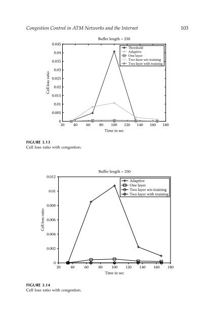
Congestion Control in ATM Networks and the Internet 103Cell loss ratio0.0450.040.0350.030.0250.020.015Buffer length = 250ThresholdAdaptiveOne layerTwo layer w/o trainingTwo layer with training0.010.005020 40 60 80 100 120 140 160 180Time in secFIGURE 3.13Cell loss ratio with congestion.0.0120.01Buffer length = 250AdaptiveOne layerTwo layer w/o trainingTwo layer with training0.008Cell loss ratio0.0060.0040.002020 40 60 80 100Time in sec120 140 160 180FIGURE 3.14Cell loss ratio with congestion.
104 Wireless Ad Hoc and Sensor NetworksMoreover, it is observed that the two-layer NN method performed betterin providing a low CLR during congestion, compared to the adaptiveARMAX, threshold, and one-layer methods. However, as expected, themultilayer NN method takes longer to transfer cells from the source tothe destination compared to the open-loop scenario. In addition, providingoffline training did indeed reduce the cell-transfer delay, whereas theCLR is still near zero. From the figures, it is clear that the CLR resultingfrom the two-layer NN method outperforms the adaptive, thresholding,and one-layer NN methods. Finally, the overall delay observed for twolayerNN was within 1% of the total transmission time of 167 sec, whereasother schemes took longer than 3%.Figure 3.15 and Figure 3.16 present the buffer utilization using adaptiveARMAX, one-layer NN, multilayer NN with and without a priori training.The buffer utilization is very low for the thresholding method because ofa threshold value of 40%, whereas the one-layer NN stores cells in thebuffer frequently resulting in a very high utilization. The multilayer NNwithout a priori training does not utilize the buffer as much as the multilayerNN with training. This is due to the inaccurate knowledge of thetraffic flow with no a priori training. Also, as more buffer space is providedto the multilayer NN with no a priori training, the utilization increaseswith buffer size. However, as pointed out earlier, the overall delay issmaller than other schemes even though the queuing delay is slightlyhigher.100Feedback delay = 0Buffer utilization9080706050ThresholdAdaptiveOne layerTwo layer w/o trainingTwo layer with training4030150 200 250 300 350Buffer length (cells)FIGURE 3.15Cell loss ratio with congestion.
- Page 76 and 77: Background 53with x( 0)being the in
- Page 78 and 79: Background 55with tr(.) the matrix
- Page 80 and 81: Background 57nGiven a function ft (
- Page 82 and 83: Background 592.3.2 Lyapunov Stabili
- Page 84 and 85: Background 61as well as Jagannathan
- Page 86 and 87: Background 63The subsequent example
- Page 88 and 89: Background 65Evaluating this along
- Page 90 and 91: Background 67Now, select the feedba
- Page 92 and 93: Background 69is SISL if and only if
- Page 94 and 95: Background 71L 1 (x)L(x, t)L 0 (x)0
- Page 96 and 97: Background 73for some R > 0 such th
- Page 98 and 99: Background 75Evaluating the first d
- Page 100: Background 77Section 2.4Problem 2.4
- Page 103 and 104: 80 Wireless Ad Hoc and Sensor Netwo
- Page 105 and 106: 82 Wireless Ad Hoc and Sensor Netwo
- Page 107 and 108: 84 Wireless Ad Hoc and Sensor Netwo
- Page 109 and 110: 86 Wireless Ad Hoc and Sensor Netwo
- Page 111 and 112: 88 Wireless Ad Hoc and Sensor Netwo
- Page 113 and 114: 90 Wireless Ad Hoc and Sensor Netwo
- Page 115 and 116: 92 Wireless Ad Hoc and Sensor Netwo
- Page 117 and 118: 94 Wireless Ad Hoc and Sensor Netwo
- Page 119 and 120: 96 Wireless Ad Hoc and Sensor Netwo
- Page 121 and 122: 98 Wireless Ad Hoc and Sensor Netwo
- Page 123 and 124: 100 Wireless Ad Hoc and Sensor Netw
- Page 125: 102 Wireless Ad Hoc and Sensor Netw
- Page 129 and 130: 106 Wireless Ad Hoc and Sensor Netw
- Page 131 and 132: 108 Wireless Ad Hoc and Sensor Netw
- Page 133 and 134: 110 Wireless Ad Hoc and Sensor Netw
- Page 135 and 136: 112 Wireless Ad Hoc and Sensor Netw
- Page 137 and 138: 114 Wireless Ad Hoc and Sensor Netw
- Page 139 and 140: 116 Wireless Ad Hoc and Sensor Netw
- Page 141 and 142: 118 Wireless Ad Hoc and Sensor Netw
- Page 143 and 144: 120 Wireless Ad Hoc and Sensor Netw
- Page 145 and 146: 122 Wireless Ad Hoc and Sensor Netw
- Page 147 and 148: 124 Wireless Ad Hoc and Sensor Netw
- Page 149 and 150: 126 Wireless Ad Hoc and Sensor Netw
- Page 151 and 152: 128 Wireless Ad Hoc and Sensor Netw
- Page 153 and 154: 130 Wireless Ad Hoc and Sensor Netw
- Page 155 and 156: 132 Wireless Ad Hoc and Sensor Netw
- Page 157 and 158: 134 Wireless Ad Hoc and Sensor Netw
- Page 159 and 160: 136 Wireless Ad Hoc and Sensor Netw
- Page 161 and 162: 138 Wireless Ad Hoc and Sensor Netw
- Page 163 and 164: 140 Wireless Ad Hoc and Sensor Netw
- Page 165 and 166: 142 Wireless Ad Hoc and Sensor Netw
- Page 167 and 168: 144 Wireless Ad Hoc and Sensor Netw
- Page 170 and 171: 4Admission Controller Design for Hi
- Page 172 and 173: Admission Controller Design for Hig
- Page 174 and 175: Admission Controller Design for Hig
Congestion Control in ATM <strong>Networks</strong> <strong>and</strong> the Internet 103Cell loss ratio0.0450.040.0350.030.0250.020.015Buffer length = 250Threshold<strong>Ad</strong>aptiveOne layerTwo layer w/o trainingTwo layer with training0.010.005020 40 60 80 100 120 140 160 180Time in secFIGURE 3.13Cell loss ratio with congestion.0.0120.01Buffer length = 250<strong>Ad</strong>aptiveOne layerTwo layer w/o trainingTwo layer with training0.008Cell loss ratio0.0060.0040.002020 40 60 80 100Time in sec120 140 160 180FIGURE 3.14Cell loss ratio with congestion.


