Predict Failures: Crow-AMSAA 101 and Weibull 101 - Barringer and ...
Predict Failures: Crow-AMSAA 101 and Weibull 101 - Barringer and ... Predict Failures: Crow-AMSAA 101 and Weibull 101 - Barringer and ...
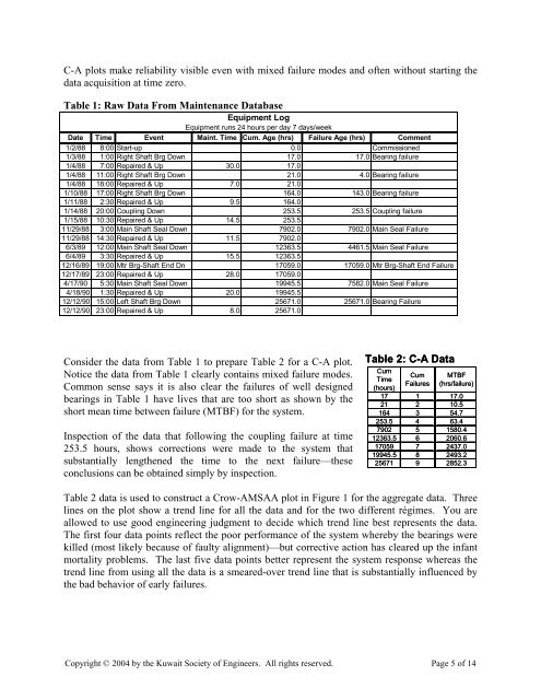
C-A plots make reliability visible even with mixed failure modes and often without starting thedata acquisition at time zero.Table 1: Raw Data From Maintenance DatabaseEquipment LogEquipment runs 24 hours per day 7 days/weekDate Time Event Maint. Time Cum. Age (hrs) Failure Age (hrs) Comment1/2/88 8:00 Start-up 0.0 Commissioned1/3/88 1:00 Right Shaft Brg Down 17.0 17.0 Bearing failure1/4/88 7:00 Repaired & Up 30.0 17.01/4/88 11:00 Right Shaft Brg Down 21.0 4.0 Bearing failure1/4/88 18:00 Repaired & Up 7.0 21.01/10/88 17:00 Right Shaft Brg Down 164.0 143.0 Bearing failure1/11/88 2:30 Repaired & Up 9.5 164.01/14/88 20:00 Coupling Down 253.5 253.5 Coupling failure1/15/88 10:30 Repaired & Up 14.5 253.511/29/88 3:00 Main Shaft Seal Down 7902.0 7902.0 Main Seal Failure11/29/88 14:30 Repaired & Up 11.5 7902.06/3/89 12:00 Main Shaft Seal Down 12363.5 4461.5 Main Seal Failure6/4/89 3:30 Repaired & Up 15.5 12363.512/16/89 19:00 Mtr Brg-Shaft End Dn 17059.0 17059.0 Mtr Brg-Shaft End Failure12/17/89 23:00 Repaired & Up 28.0 17059.04/17/90 5:30 Main Shaft Seal Down 19945.5 7582.0 Main Seal Failure4/18/90 1:30 Repaired & Up 20.0 19945.512/12/90 15:00 Left Shaft Brg Down 25671.0 25671.0 Bearing Failure12/12/90 23:00 Repaired & Up 8.0 25671.0Consider the data from Table 1 to prepare Table 2 for a C-A plot.Notice the data from Table 1 clearly contains mixed failure modes.Common sense says it is also clear the failures of well designedbearings in Table 1 have lives that are too short as shown by theshort mean time between failure (MTBF) for the system.Inspection of the data that following the coupling failure at time253.5 hours, shows corrections were made to the system thatsubstantially lengthened the time to the next failure—theseconclusions can be obtained simply by inspection.Table 2: C-A DataCumCumMTBFTimeFailures(hrs/failure)(hours)17 1 17.021 2 10.5164 3 54.7253.5 4 63.47902 5 1580.412363.5 6 2060.617059 7 2437.019945.5 8 2493.225671 9 2852.3Table 2 data is used to construct a Crow-AMSAA plot in Figure 1 for the aggregate data. Threelines on the plot show a trend line for all the data and for the two different régimes. You areallowed to use good engineering judgment to decide which trend line best represents the data.The first four data points reflect the poor performance of the system whereby the bearings werekilled (most likely because of faulty alignment)—but corrective action has cleared up the infantmortality problems. The last five data points better represent the system response whereas thetrend line from using all the data is a smeared-over trend line that is substantially influenced bythe bad behavior of early failures.Copyright © 2004 by the Kuwait Society of Engineers. All rights reserved. Page 5 of 14
Figure 1: Crow-AMSAA Plot Of Data From Table 2The early failures are represented by the statistics λ=0.5596 and β=0.355 for the “ancient”history. We have little interest in this phase of the data as corrective actions have beenimplemented.The most current history is represented by the statistics λ=0.05116 and β=0.509 which will beused to make a “fearless forecast” of future failures for the system using the equationN(t)=λ*t β . Solving the equation for cumulative time gives t=(N(t)/λ) (1/β) . We can forecast thenext failure, failure number 10, will occur at t=(10/0.05116) (1/0.509) = 31704.3 hours which isforecasted as 31704.3 – 25671 = 6033.3 hours into the future.Skeptics will now say you cannotforecast the future with anyaccuracy. So simply try thisexperiment using the data in Table2 as unfolded in Table 3 as thedataset develops over time. Theforecasted failures are roughlywithin 10% of the actualcumulative times as observedfrom the error data—more dataTable 3: C-A Forecast Using Small Data SetCumCumCumCumCumCumTimeTimeTimeFailuresFailuresFailures(hours)(hours)(hours)12363.5 6 12363.5 6 12363.5 617059 7 17059 7 17059 719945.5 8 19945.5 825671 9λ = 0.06587 0.01836 0.05116β= 0.479 0.614 0.509Fcst (hrs) = 22468.3 8 24083.0 9 31704.3 10∆ Time (hrs)= 5409.3 4137.5 6033.3Error (hrs)= 2522.8 -1588.0 ?Copyright © 2004 by the Kuwait Society of Engineers. All rights reserved. Page 6 of 14
- Page 1: Predict Failures:Crow-AMSAA 101 and
- Page 5: Seventy years ago we accepted that
- Page 9 and 10: humans are involved in the safety i
- Page 11 and 12: the time interval. The plots are
- Page 13 and 14: Figure 5: Weibull Plot Showing Infa
- Page 15: Using the range of beta valuesfrom
C-A plots make reliability visible even with mixed failure modes <strong>and</strong> often without starting thedata acquisition at time zero.Table 1: Raw Data From Maintenance DatabaseEquipment LogEquipment runs 24 hours per day 7 days/weekDate Time Event Maint. Time Cum. Age (hrs) Failure Age (hrs) Comment1/2/88 8:00 Start-up 0.0 Commissioned1/3/88 1:00 Right Shaft Brg Down 17.0 17.0 Bearing failure1/4/88 7:00 Repaired & Up 30.0 17.01/4/88 11:00 Right Shaft Brg Down 21.0 4.0 Bearing failure1/4/88 18:00 Repaired & Up 7.0 21.01/10/88 17:00 Right Shaft Brg Down 164.0 143.0 Bearing failure1/11/88 2:30 Repaired & Up 9.5 164.01/14/88 20:00 Coupling Down 253.5 253.5 Coupling failure1/15/88 10:30 Repaired & Up 14.5 253.511/29/88 3:00 Main Shaft Seal Down 7902.0 7902.0 Main Seal Failure11/29/88 14:30 Repaired & Up 11.5 7902.06/3/89 12:00 Main Shaft Seal Down 12363.5 4461.5 Main Seal Failure6/4/89 3:30 Repaired & Up 15.5 12363.512/16/89 19:00 Mtr Brg-Shaft End Dn 17059.0 17059.0 Mtr Brg-Shaft End Failure12/17/89 23:00 Repaired & Up 28.0 17059.04/17/90 5:30 Main Shaft Seal Down 19945.5 7582.0 Main Seal Failure4/18/90 1:30 Repaired & Up 20.0 19945.512/12/90 15:00 Left Shaft Brg Down 25671.0 25671.0 Bearing Failure12/12/90 23:00 Repaired & Up 8.0 25671.0Consider the data from Table 1 to prepare Table 2 for a C-A plot.Notice the data from Table 1 clearly contains mixed failure modes.Common sense says it is also clear the failures of well designedbearings in Table 1 have lives that are too short as shown by theshort mean time between failure (MTBF) for the system.Inspection of the data that following the coupling failure at time253.5 hours, shows corrections were made to the system thatsubstantially lengthened the time to the next failure—theseconclusions can be obtained simply by inspection.Table 2: C-A DataCumCumMTBFTime<strong>Failures</strong>(hrs/failure)(hours)17 1 17.021 2 10.5164 3 54.7253.5 4 63.47902 5 1580.412363.5 6 2060.617059 7 2437.019945.5 8 2493.225671 9 2852.3Table 2 data is used to construct a <strong>Crow</strong>-<strong>AMSAA</strong> plot in Figure 1 for the aggregate data. Threelines on the plot show a trend line for all the data <strong>and</strong> for the two different régimes. You areallowed to use good engineering judgment to decide which trend line best represents the data.The first four data points reflect the poor performance of the system whereby the bearings werekilled (most likely because of faulty alignment)—but corrective action has cleared up the infantmortality problems. The last five data points better represent the system response whereas thetrend line from using all the data is a smeared-over trend line that is substantially influenced bythe bad behavior of early failures.Copyright © 2004 by the Kuwait Society of Engineers. All rights reserved. Page 5 of 14


