A Priority-Based Model of Routing - Chicago Journal of Theoretical ...

A Priority-Based Model of RoutingBabak Farzad, Neil Olver and Adrian Vetta ∗February 5, 2008AbstractWe consider a priority-based selfish routing model, where agents may have differentpriorities on a link. An agent with a higher priority on a link can traverse it with asmaller delay or cost than an agent with lower priority. This general framework can beused to model a number of different problems. The structural properties that lead toinefficiencies in routing choices appear different in this priority-based model comparedto the classical model. In particular, in parallel link networks with nonatomic agents,the price of anarchy is exactly one in the priority-based model; that is, selfish behaviourleads to optimal routings. In contrast, in the standard model the worst possible price ofanarchy can be achieved in a simple two-link network. For multi-commodity networks,selfish routing does lead to inefficiencies in the priority-based model. We present tightbounds on the price of anarchy for such networks. Specifically, in the nonatomic casethe worst-case price of anarchy is exactly (d + 1) d+1 for polynomial latency functionsof degree d (hence 4 for linear cost functions). For atomic games, the worst-case priceof anarchy is exactly 3 + 2 √ 2 in the weighted case, and exactly 17/3 in the unweightedcase. An upper bound of O(2 d d d ) is also shown for polynomial cost functions in theatomic case, although this is not tight. Our framework (and results) also generalise toinclude models similar to congestion games.ACM Classification: F.2.0, F.2.2AMS Classification: 68Q25, 68M10, 90B18Key words and phrases: selfish routing, price of anarchy1 IntroductionThis work is motivated by the simple observation that, in a transportation network, a cartraversing a road can only cause congestion delays to those cars that use the road at a latertime. Moreover, this is a common feature of most traffic networks and queuing models.The study of congestion and transportation networks is not new. The ideas were firstdiscussed qualitatively by Pigou [14] in 1920, and later placed on a sound mathematicalfooting by Wardrop [20]. The book of Beckmann, McGuire and Winsten [4] gives a verythorough treatment. More recently, applications to communication networks such as the∗ McGill University. Email: {babak,olver,vetta}@math.mcgill.ca1

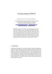
f e (x e )f e (x (j)e )x (j)ex eFigure 1: Classical versus priority-based selfish routinginternet spurred interest from the computer science community. The concept of the price ofanarchy was introduced by Koutsoupias and Papadimitriou [12]. It is the ratio between thecosts of the worst Nash equilibrium and the optimal routing, and is essentially a quantitativemeasure of the loss of efficiency attributable to the lack of a central coordinating authority.In this classical selfish routing model, each link e has an associated cost function f e (x);the delay experienced by the users of this link is then f e (x e ), where x e is the total trafficon the link. Thus all users of a link experience the same latency. One practical situation inwhich this may arise is when users are continuously using a network, making the conceptof time redundant. There are many situations where this assumption is not valid however.For example, imagine someone driving home during rush hour in a large city. The timethat they leave will make a big difference to how long the trip takes; it will be much shorterif they leave early enough to avoid the worst of the traffic.Here we show that a simple modification to the classical model does allow us to incorporatesome elements of time dependence. In the classical model, the total cost associatedwith a link e is the delay experienced on that link, multiplied by the number of playersusing it, i.e. f e (x e )x e . In our model, the total cost will instead be given by the area underthe cost function, i.e. the integral ∫ x e0f e (z)dz. The idea is that the area under the costfunction can be partitioned amongst the users so that earlier users are associated withsmaller latencies. If a player j has an amount x (j)e of flow ahead of it, it will experience adelay of f e (x (j)e ). The difference between the models is represented visually in Figure 1; thetotal cost associated with link e in the classical model is given by the area of the lightlyshaded rectangle, and in the priority-based model it is given by the area under the curve.There are other reasons aside from time-based considerations why different users mightexperience different delays or costs; for instance, certain users might simply be given priority,and always experience lower latencies. Our model allows the ordering of the playersto be defined very generally; various examples will be discussed later.Both the classical and priority-based models can be broadly divided into two variants;atomic and nonatomic. In the atomic case, there are a finite number of agents, each with acertain amount of flow to route. The flow may be splittable, or unsplittable, in which case2

each agent must pick a single path for its entire flow. In the nonatomic case, there are aninfinite number of agents, and each controls only a negligible fraction of the total flow. Theresults and techniques will be different for these two variants; the atomic case is generallymore difficult to analyse.This simple modification of using an integral rather than a rectangle to measure the coston a link has more of an effect than one might expect. Roughgarden and Tardos [18, 16]showed that in the classical model with nonatomic agents, the worst-case price of anarchyis 4/3 for linear cost functions, and (1 − d(d + 1) −1−1/d ) −1 = Θ(d log d) for polynomial costfunctions of degree d. By contrast, we show that in the nonatomic priority-based model,the worst-case price of anarchy is exactly 4 for linear cost functions, and (d + 1) d+1 forpolynomial cost functions of degree d; these are considerably larger.In addition, some of the causes of the inefficiencies due to selfish routing appear tobe different. In particular, it is known [16] that even in single-commodity networks (infact, even in simple parallel link networks), the above worst-case bounds in the standardnonatomic model can be achieved. Thus the worst-case price of anarchy is essentiallyindependent of the network topology in the standard model. By contrast, we will showthat selfish routing leads to optimal solutions in parallel link networks in the priority-basedmodel, for any choice of priority scheme. For some important special cases of our model(including the time-based model mentioned earlier), this is still true for arbitrary singlecommoditynetworks, where all agents have the same origin and destination.The atomic unsplittable case of the classical model was considered by Azar, Awerbuchand Epstein [3]. They show that for linear cost functions, (3+ √ 5)/2 is a tight upper boundfor the price of anarchy; this is reduced to 2.5 in the unweighted case, where all users routeone unit of demand (see Christodoulou and Koutsoupias [5] for an independent proof). Weshow that in the priority-based model with linear cost functions, the worst-case price ofanarchy is 3 + 2 √ 2, and reduces to 17/3 in the unweighted case. They also show that forpolynomial cost functions of degree d, the worst possible price of anarchy is d Θ(d) ; this waslater determined exactly by Aland et al. [2] (see also Olver [13]). We show an upper boundof O(2 d d d ) in our model for this case.Related work Rosenthal [15] introduced atomic selfish routing games, as well as congestiongames, an important generalisation which removes the network structure. Our modelgeneralises in an analogous way.Correa, Schulz and Stier-Moses [6] gave shorter proofs of some of the price of anarchyresults for nonatomic games, as well as some new results. Some of our proofs are inspiredby their technique.Independently of this work, Harks, Heinz and Pfetsch [9] consider an online versionof the multicommodity routing problem. The greedy online algorithm they consider canbe interpreted as the Nash equilibrium in an instance of what we call the global prioritymodel, a special case of the priority-based model. Thus price of anarchy results in theglobal priority model are related to online competitiveness results in their model. Harksand Végh [10] generalise [9] to an online selfish routing game; in this game, a sequence ofstandard selfish routing games are played, and players in a particular game are aware ofthe choices made by the players in earlier games, but not later ones. This model are insome sense a generalisation of the global priority model where some players have identical3

priorities.Paper outline In Section 2 we present the priority-based selfish routing model, consideringatomic and nonatomic agents. We also give a number of motivating applications, and showsome sufficient conditions for the existence of Nash equilibria. The bulk of the paper isdevoted to deriving the exact value for the price of anarchy under certain restrictions onthe cost functions. In Section 3, we consider the price of anarchy of nonatomic agents;single-commodity networks are considered first, followed by the general multicommoditycase. Atomic agents are dealt with in Section 4.2 The ModelWe now define the model rigorously. We begin with the atomic unsplittable case, since thisis actually easier to define (although more difficult to analyse).2.1 The unsplittable atomic caseWe begin with a network, represented as a directed graph G = (V, E), and a finite numbern of players. Each player j has a flow requirement of w j units, which must be routed fromnode s j to node t j . The players must each pick a single path to route their entire demand.A particular routing is then defined by P = {P 1 , . . .,P n }, where P j is an s j − t j path foreach j, representing the route taken by that player. We also define the flow vector x(P) byx e (P) = ∑ j:e∈P jw j , the total flow on edge e. We will write simply x e if the desired routingis clear. Each edge has an associated cost function f e that is nonnegative and increasing.We will also sometimes refer to these as latency functions, since they represent the delayexperienced by the user on the edge. So far, nothing we have described differs from thestandard network routing model. But now we introduce a priority scheme that will allowus to order the users of a particular edge, prescribing different latencies to the users basedon this order. We will allow this to be very general—the priority ordering on an edge candepend arbitrarily on the current routing P. This can include dependence on routings thatdo not use that edge. If player i has higher priority than player j on edge e under routingP, we write i ≻ P,e j. For a fixed e and P , the relation ≻ P,e must define a total orderingof the players using edge e; this is the only restriction we impose. If it is clear from thecontext what edge or routing is being referred to, we will omit it.For an arbitrarily defined priority scheme, it might not be computationally feasibleto calculate a player’s best response, since there are an exponential number of paths toconsider and the priority orderings could be different for all of them. In that case, bestresponse dynamics and Nash equilibria would not be of much practical interest. Manynatural priority schemes that we consider do allow best responses to be easily calculated.For example, one possibility would be to give an ordering to the players, and assign thepriority along all the edges based on this ordering. Another option would be to assignpriorities based on the time that the players arrive at the beginning of the link. We willdescribe in detail a number of possible priority schemes, including these ones, in Section 2.2.In the classical selfish routing model, the total (or social) cost of a routing is givenby C(P) = ∑ e∈E f e(x e )x e . As mentioned in the introduction, we will modify this in our4

2.2 Some possible priority schemesHere we list some natural and interesting games that fall within the framework of ourmodel, by picking the priority scheme appropriately.The global priority game This is the simplest possible case; the ordering is independentof the routing, and is also the same for all edges. In other words, there is a fixed priorityordering of the players.This model has an interesting interpretation as an online routing problem, as discussedby Harks et al. [9]. Suppose players are charged for their use of a network, and would liketo choose the cheapest route for their demand. The players arrive one at a time however,and the amount charged to a player for using an edge depends on the current congestionon the edge; later players may be charged more for some edges than earlier players. Thesocial optimum is taken to be the total cost incurred by all the players. In this setting, aNash equilibrium can be interpreted as a greedy online algorithm, and the price of anarchycorresponds to the competitiveness of this algorithm. Most of the results in Harks et al.correspond to the atomic model, but with splittable flow; for instance, they show thatwith n unweighted splittable players, and linear cost functions, the price of anarchy cannotexceed 4n/(2 + n).The fixed priority game A more general model than the global priority one, herewe still insist that the priorities are independent of the routing, but we allow differentorderings on different edges. One application within this framework is Quality of Servicein telecommunication networks such as the internet. In the absence of network neutrality,telecommunication companies could charge for faster access to the portion of the internetthat they own. The players in this case would be companies with a large internet presence;these companies want to serve content to their users as quickly as possible. The prioritieswould then be determined by contracts between the companies and the service providers.The timestamp game The priorities of agents are determined by their arrival times atthe start of the edge. Associate with each agent j an additional value τ j that representsthe starting time of that agent. Now take a specific routing P = {P 1 , . . .,P n }. The timeagent j arrives at a vertex u ∈ P j is then τ j plus the time taken to traverse all the edgeson the subpath of P j from s j to u, denoted P j [s j , u].Of course, the latency of player j along an edge in P j [s j , u] depends on the priority ofj on that edge, which in turn depends on the start times of other agents. To see that wehave enough information to uniquely determine the priorities, imagine simulating the game.Take the player with the smallest starting time, and move her along the first edge of herpath. Her timestamp is then adjusted to include the time taken to traverse this edge. Wethen repeat, taking the player with the smallest timestamp after this update (this couldbe the same player). When the simulation terminates and all players have reached theirdestinations, we can read off the priority ordering on any edge; it is simply the order inwhich the players traversed that edge in the simulation.The technical issue of ties—two agents taking the same edge with the same timestamp—can easily be resolved, either by prescribing a tie-breaking order for the players, or byperturbing the starting times by sufficiently small values to break the ties without modifyingthe ordering.6

One problem with this model is that a player using a link delays all players that traversethe link afterwards. This is not very realistic—rather, the delaying effect of a playershould only last for a short time. Congestion effects, however, complicate the situation;the duration of the delaying effect can vary quite dramatically depending on the situation.If a link is heavily congested, a player might delayed by traffic from quite some time ago.A better model could be obtained using a proper model of flow over time, where packetshave a well defined position at each moment in time, and so the amount of traffic on anedge can vary. Such a “dynamic” model was introduced by Ford and Fulkerson [7], and hasreceived considerable attention. Köhler and Skutella [11] have proposed a dynamic modelwith load-dependent transit times which can incorporate congestion effects. Investigatingthe behaviour of such a dynamic model with selfish behaviour would be an interestingavenue of research.For the congestion game variant of our model, the following is one motivating example:The subcontractor game Suppose there are a number of construction companies, eachinvolved with one or more large project. In order to complete various parts of these projects,the construction companies need to enlist the services of subcontractors. There are manysubcontractors to choose from, and different subcontractors provide different subsets ofservices (more than one subcontractor may offer the same service). Also, there might bemore than one way of completing a project, and so the construction company might havea choice of which services are required. However, if two companies decide to use the samesubcontractor, and require some of the same services, the subcontractor will not be ableto complete both requests simultaneously. A delay in construction will negatively affectthe profit of the construction company, so essentially the company that gets delayed ispaying more for the service. 1 The subcontractor’s choice as to which company to delaycould depend on many factors—the time that the contracts were made, the total value ofthe contracts, previous business relationships with the companies, etc.To model this as a priority-based congestion game, we will consider each company as anagent, and each service offered by a subcontractor as an item (the same service offered bymultiple contractors will considered as multiple items). The possible strategies for an agentwill then be any combination of services from the subcontractors that together provide allthe needs of the agent. Since our model is so general, the priority ordering could be ascomplicated as needed to take the various factors noted above into account.2.3 The nonatomic caseIf we let the fraction of the total flow controlled by any single player diminish to zero,the game becomes nonatomic. We have to be quite careful in defining things formallyhowever—there are some subtleties that do not occur in the standard model. Our approachto nonatomic games follows Schmeidler [19], in that the game is represented by an atomlessspace of players, and each player has an associated payoff function.Label the players by elements in the interval R = [0, 1]. We also have two measurable1 Alternatively, the subcontractor may experience increasing marginal costs; for example, these may bedue to overtime payments, increased costs arising from the need for additional production, etc. Theseadditional costs are then passed on to the construction companies.7

functions s, t : R → V , which specify the origin and destination of each player respectively.For each r ∈ [0, 1], the strategy of player r is given by a unit s r − t r flow y r . We areallowing splittable flow—the reason for this is discussed later in this section. A feasiblesolution is given by P = {y r : r ∈ R}. A priority ordering is defined as before; for any edgee and feasible solution P, ≻ P,e is a total ordering of the players.The total flow on edge e will then be x e = ∫ R y r(e)dµ. The amount of flow on edge eahead of player r is given by∫x e (r) (P) =L (r)e (P)y s (e)dµ,where L e (r) (P) = {s : s ≻ P,e r}. We require that L e (r) (P) be Lebesgue measurable for alle ∈ E, r ∈ R and feasible P; any reasonable ordering will satisfy this technical requirement.The total latency experienced by player r, i.e. the time taken for the player to traversefrom the source to the sink, isl r (P) = ∑ ( )f e x e (r) (P) . (4)e∈P rAnalogously to the atomic case, the requirement for P to be a Nash equilibrium is that forany r ∈ R and any s r − t r path P ′ ,l r (P) ≤ l r (P ′ ) (5)where P ′ = P\P j ∪ P ′ .The model is most easily thought of as a nonatomic version with splittable flow. There isa reason for this; in general, we cannot assign an unsplittable flow to each nonatomic player.For consider a simple two-link network with arcs e and e ′ , and define the cost functionsf e (x) = f e ′(x) = x. Assign the global priority ordering r ≻ s iff r < s. Now suppose wedemand that each player routes an unsplittable flow; consider any such solution P wherethe flows y r are all 0 − 1 vectors. Any Nash equilibrium must satisfy x e(r)all r ∈ R. Now define F = {s ∈ R : y r (e) = 1}. Thenx (r)e =∫Ry s (e)1 s≻r dµ = µ(F ∩ [0, r]).= x (r)e ′= r/2 forThis implies that µ(F ∩ [r, s]) = (s − r)/2 for all [r, s] ⊂ [0, 1]. This however contradictsLebesgue’s density theorem, which states that a measurable set has density 1 almost everywherein the set. Thus even in this very simple example, no Nash equilibrium existswith unsplittable flow. On the other hand, setting y r (e) = y r (e ′ ) = 1/2 for all r is a Nashequilibrium.The nonatomic case in the classical model is comparatively much easier to define. Inthe classical model, a solution is defined completely by the flow vector x—only the totalflow on an edge is important. Such games, where each player’s payoff depends only onthe aggregate action of the other players, have some useful simplifying properties (see e.g.Schmeidler [19]).It might not be clear then why this nonatomic game can be considered a suitable limitof the atomic unsplittable game when w j → 0. For some intuition, take again this simple8

two-link example, but with atomic agents; suppose we have n agents (labelled from 1 ton), all of size 1/n, going from the origin to the destination; the priority ordering is i ≻ jiff i < j. Then one possible Nash equilibrium is for odd-numbered players to take arc e,and all even-numbered players to take edge e ′ ; call this solution P n . Considering the set ofstrategies, this does not lead to any sensible limit as n → ∞. For a fixed r ∈ [0, 1], we dohowever have thatlim (P n ) = r/2.n→∞ x(⌊rn⌋) eIn that sense, we converge to the Nash equilibrium of the nonatomic game as we havedefined it.Generalising to congestion games is done analogously to the atomic case.2.4 Existence of Nash equilibriaWe mention a few existence and nonexistence results regarding pure Nash equilibria. First,an unsurprising negative result; in the atomic unsplittable case, allowing general priorityschemes, there need not be a pure Nash equilibrium. In particular, consider the fixedpriority game depicted in Figure 2. The edges in this network are undirected, and flow ineither direction contributes to the congestion on an edge. this point shortly). There aretwo users, each of size 1, with source-destination pairs (s 1 , t 1 ) and (s 2 , t 2 ) respectively. Alledges have cost function f e (x) = x. The priorities on each edge are shown in the figure. Itis easy to see that no matter which direction each of the two players choose to route theirflow, the player with lower priority on the single edge these routes have in common willhave an incentive to change to the other route. Thus the game has no pure Nash equilibria.Since this example is unweighted, this is in contrast with the classical mode; unweightedatomic congestion games always have a pure Nash equilibrium (but weighted ones neednot) [15].s 12 ≻ 1s 2t 22 ≻ 1t 11 ≻ 2 1 ≻ 2Figure 2: A fixed-priority game with no pure Nash equilibria.Of course, we have not explicitly allowed undirected edges in our model. But we canreplace each of the undirected edges in the construction with the widget shown in Figure 3;v and w represent the endpoints of the replaced edge (this is a standard technique; seee.g. [1]).Now for a positive result: in the global priority model, even in the atomic unsplittablecase, there is always a pure Nash equilibrium (as long as the cost functions are at leastnonnegative and increasing). This can be seen in the atomic case by an explicit algorithmto construct the Nash: simply go through the agents in priority order, and route each along9

Proof. This follows by noting that the cost of a flow x in the priority-based model,C(x) = ∑ e∈E∫ xe0f e (x)dx,is exactly the same as the cost induced in the classical model with cost functions ˆf e :Ĉ(x) = ∑ e∈Eˆf e (x e )x e = ∑ e∈E∫ xe0f e (x)dx.Corollary 2.3. In a nonatomic priority-based game, the optimal flows are exactly theWardrop equilibria of the classical network game on the same network, with the same costfunctions.Proof. The result follows directly from the following characterisation of optimal flows inthe classical model [4, 14, 17]:A flow x is optimal for a classical nonatomic game with continuously differentiable,semiconvex 2 cost functions ˆf e iff it is a Wardrop equilibrium for a game on the samenetwork, where the cost functions are replaced byfe ∗ (y) = d (y ·dyˆf)e (y) .But if the ˆf e ’s are defined as in Equation (6), then f ∗ e (y) = f e (y), and the result follows.3 The price of anarchy of nonatomic agentsThe central topic of this paper is the question: how bad can the cost of a Nash equilibriumbe compared to the cost of an optimal solution? The price of anarchy is a quantitativeanswer to this question:Definition 2. The (pure) price of anarchy of an instance is the ratio between the cost ofthe worst possible pure Nash equilibrium, and the cost of the optimal solution.An analogous definition can be made for mixed Nash equilibria; however, we will onlyconsider pure Nash equilibria in this paper. As such, we will usually omit “pure”. We willalso use the term worst-case price of anarchy in relation to a class of possible instances (forexample, all instances with linear cost functions) to refer to the supremum of the price ofanarchy over all these instances.Analysing the price of anarchy is easier in the nonatomic case, where there are aninfinite number of players, each controlling a negligible amount of flow. The special case ofsingle-commodity networks (particularly parallel link networks) give very different resultsto general networks, and we discuss these separately.2 A function f(y) is semiconvex iff yf(y) is convex.11

3.1 Single-commodity networksSingle-commodity networks refer to the case where all agents have the same source s anddestination t. We only require the cost functions be continuous, nonnegative and increasingfor the following results.Observation 1. For a single-commodity game with nonatomic agents, any flow x whereall of the s − t paths with non-zero flow are shortest paths (where length is determinedby the metric l e = f e (x e )) is a Wardrop equilibrium in the classical model, and hence byCorollary 2.3, an optimal flow in the priority-based model. In other words, a flow satisfying∑f e (x e ) ≤ ∑ f e (x e ). (7)e∈P ′e∈Pfor any s − t path P with x P > 0, and all s − t paths P ′ , is optimal.A particularly simple class of networks of this type are parallel link networks, whichconsist only of a source node, a sink node, and some number of links between them. Weshow the following:Theorem 3.1. For parallel link networks with nonatomic agents and any choice of priorityscheme, the price of anarchy is one.Proof. Let P be an arbitrary Nash equilibrium. Consider Equation (5). In our case, it canbe writtenl r (P) ≤ f e ′(x (r)e ′ ) for all e ′ ∈ E, (8)for all players r. Now for each link e, either x e = 0 or there is a player r such that P r = eand x e(r) = x e . Equation (8) then yieldsHence the result follows by Observation 1.f e (x e ) ≤ f e ′(x e ′) for all e ′ ∈ E.We can obtain a similar result for general single-commodity networks if we restrict thepriority scheme:Theorem 3.2. The nonatomic versions of both the global priority and timestamp gameshave a price of anarchy of one in single-commodity networks.Proof. We first show that in the single-commodity case, the timestamp game is exactlyequivalent to the global priority game. Take any two players r, s ∈ R whose routes in theNash routing P intersect, and where the start times satisfy τ r < τ s . Then for any edgee ∈ P r ∩P s , r must arrive at the start of this edge earlier than s. For if not, r could changeher route to be the same as s’s route until edge e, hence arriving earlier and contradictingthe Nash requirement.So we need consider only the global priority game. Take any path P on which P hasnon-zero flow. Consider player r, the lowest priority agent that takes path P. Since we areat Nash, this player has no incentive to switch; in particular, l r (P) ≤ ∑ e∈P ′ f e(x e ) for anys − t path P ′ . Thus Observation 1 applies, and P is an optimal routing.12

These results are in contrast to the classical model, where Pigou’s two-link networkyields the largest possible price of anarchy in most cases [16]. A natural question is whetherthe Nash solution in our model is always optimal, but this is not the case. The followingexample shows this for the fixed priority game (even for single-commodity flow), and laterwe will show it for other variants of the model.Consider the simple network shown in Figure 4. Take R = [0, 1] for the set of players,and set all the cost functions to x. For those edges marked >, the priority ordering isdefined by r ≻ s iff r > s; for the edge marked >Figure 4: A single-commodity game with price of anarchy larger than one.3.2 Multicommodity networksWe now investigate the price of anarchy of the priority-based model for general networks,where the behaviour is very different from the single-commodity case. We will obtain tightbounds for linear and polynomial cost functions.First a useful inequality:Theorem 3.3. For any Nash flow P, under any priority scheme,C(P) ≤ ∑ e∈Ef e (x e (P))x ∗ e. (9)where x ∗ is an arbitrary flow (in particular, it may be an optimum flow).Proof. We will use just x e to denote x e (P). Let P ∗ = {P ∗ r : r ∈ R} be some assignmentof paths to players that obtains the flow x ∗ (so formally, it is a valid routing such that∫r:e∈P ∗ r 1 dµ = x∗ e). Apply (5) with P ′ r = P ∗ r :l r (P) ≤ l r (P (r) )= ∑ ( )f e x e (r) (P (r) ) ,e∈P ∗ rwhere P (r) = P\P r ∪ Pr ∗ ; we have used Equation (4). Now clearly x e (r) (P (r) ) ≤ x e , sol r (P) ≤ ∑f e (x e ).e∈P ∗ r13

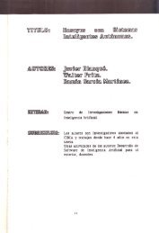
Thus∫C(P) =∫≤Rl r (P)dr∑f e (x e )drRe∈Pr∗= ∑ ∫f e (x e )e∈ER(1 e∈P ∗ r)dr= ∑ e∈Ef e (x e )x ∗ e.It is interesting to compare this to the classical model, where the variational inequality∑f e (x e )x e ≤ ∑ f e (x e )x ′ ee∈E e∈Eholds if and only if x is a Wardrop equilibrium; note that the left hand side is the cost of theflow x in the classical model. In our model, the inequality is necessary, but not sufficient.Let us now find an upper bound in the case of linear cost functions. The result issuperseded by the more general polynomial case considered next, but the proof in thelinear case is simpler and more transparent.Theorem 3.4. In the nonatomic case with linear cost functions, 4 is an upper bound onthe price of anarchy.Proof. Note the following, for any flow vector x ′ :∑f e (x ′ e)x ′ e = 2 ∑ 12 a ex ′2e + 1 2 b ex ′ ee∈E e∈E∫ x ′e≤ 2 ∑ a e x + b e dxe∈E0= 2C(x ′ ). (10)Beginning with the result of Theorem 3.3, we use a technique from [6], which they used togive a short proof of the classical price of anarchy result.C(P) ≤ ∑ e∈Ef e (x e )x ∗ eNow consider Figure 5.= ∑ f e (x ∗ e)x ∗ e + ∑ (f e (x e ) − f e (x ∗ e)) x ∗ ee∈Ee∈E≤ 2C(P ∗ ) +∑(f e (x e ) − f e (x ∗ e)) x ∗ e from (10).e∈E:x e≥x ∗ e14

f e (x e )f e (x ∗ e)x ∗ ex eFigure 5: A visual proof that (f e (x e ) − f e (x ∗ e))x ∗ e ≤ 1 4 f e(x e )x e .Clearly the area of the grey rectangle is at most 1 4Thus we obtainof the area of the large rectangle.C(P) ≤ 2C(P ∗ ) + 1 ∑f e (x e )x e4e∈E≤ 2C(P ∗ ) + 1 2 C(P),again using (10) in the final step. Thus C(P)/C(P ∗ ) ≤ 4, as required.We now extend this result to polynomial cost functions.Theorem 3.5. For the nonatomic case with polynomial cost functions of maximum degreed, there is an upper bound of (d + 1) d+1 for the price of anarchy.Proof. The proof uses a generalisation of the technique used to prove Theorem 3.4. Letα ≥ 1 be a constant to be chosen later. Let f e (x) = ∑ di=0 a e,ix i . We haveC(P) ≤ ∑ e∈Ef e (x e )x ∗ e= α ∑ f e (x ∗ e)x ∗ e + ∑e∈Ee∈E≤ α(d + 1)C(P ∗ ) +(f e (x e ) − αf e (x ∗ e))x ∗ e∑(f e (x e ) − αf e (x ∗ e)) x ∗ e (11)e∈E:f e(x e)≥αf e(x ∗ e)15

Now consider:(f e (x e ) − αf e (x ∗ e))x ∗ ef e (x e )x e= x∗ ex e− α · fe(x ∗ e)x ∗ ef e (x e )x e≤ x∗ ex e− α · min0≤i≤da e,i x ∗i+1ea e,i x i+1 e( )= x∗ e x∗ d+1− α e(since x ∗ e ≤ x e ).x e x eSince the maximum value of the function φ −αφ d+1 occurs at φ m = (α(d+1)) −1/d , an easycalculation yields(f e (x e ) − αf e (x ∗ e))x ∗ e ≤ dd + 1 · 1(α(d + 1)) 1/d · f e(x e )x e .Substituting into (11), and using ∑ e∈E f e(x e )x e ≤ (d + 1)C(P), it follows thatNow set α = (d + 1) d−1 ; this givesC(P)C(P ∗ ) ≤ α(d + 1)1 − d(α(d + 1)) −1/d.C(P)C(P ∗ ) ≤ (d + 1)d+1 .Having obtained an upper bound, we now show that it cannot be improved, by demonstratinghow to construct a game with price of anarchy arbitrarily close to this upper bound.We will need (and again later) the following useful lemma:Lemma 3.6. For a, b ≥ 0, r ≥ 1 and 0 < γ < 1,(a + b) r ≤ γ 1−r a r + (1 − γ) 1−r b r . (12)Proof.( ( a(a + b) r = γγ)( ) a r≤ γ + (1 − γ)γ( b+ (1 − γ))) r1 − γ) r(by convexity)( b1 − γ= γ 1−r a r + (1 − γ) 1−r b r .Theorem 3.7. For the nonatomic case with polynomial cost functions of maximum degreed, there is a lower bound of (d + 1) d+1 for the worst-case price of anarchy in the globalpriority model.16

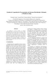
Proof sketch. Some calculations have been omitted; the full proof is given in the appendix.Consider a network of the form shown in Figure 6. There are two types of latencyfunction in the network. Each link of the form (s i , s i+1 ) has latency zero, and each linke i = (s i , t) has latency l e (x) = x d /i. We have a large number of infinitesimally small agents,all trying to get to t from one of the s i ’s. The total amount of traffic originating at each s i isunity. In addition, for all j < i all agents originating at s i have higher priority than agentsoriginating at s j . Agents originating at the same vertex are indistinguishable, except forsome fixed priority ordering among them.tl 1 (x)l 2 (x)l 3 (x)l n−1 (x)l n (x)s 10s 20s 3s n−1Figure 6: Lower bound construction for polynomial cost functions.0s nLet P n and P ∗ n be respectively the Nash equilibria and optimum solutions of this constructionfor each n.Any agent is unaffected by the choices of lower priority agents, so we can calculate theNash by working from the highest priority agents (i.e those starting from s n ) to the lowest(starting at s 1 ). Define x i,j to be the flow on the edge (s i , t) after all the players withorigins in {s j , s j+1 , . . .,s n } have played; in addition, define x i,n+1 = 0. Let y j = f ej (x j,j ).It is easy to see that the Nash condition implies thatFrom this, it can be shown thatf ei (x i,j ) = f ej (x j,j ) = y j for all i ≤ j.n∑ (C(P n ) ≥ (d + 1) d j 1/d (j + 1) −1/d − (n + 2) −1/d) d+1. (13)j=1Applying Lemma 3.6 to (13) with a = (j + 1) −1/d − (n + 2) −1/d , b = (n + 2) −1/d andr = d + 1, we obtain that for any constant 0 < γ < 1,⎛⎞n∑( ) γ d n∑C(P n ) ≥ (d + 1) d ⎝γ d j −1 (1 + 1 j )−1−1/d − (n + 2) −1−1/d j 1/d ⎠.1 − γj=1j=1Some calculations then show thatC(P n ) ≥ γ d (d + 1) d H n − D γ ,where D γ is a constant that depends on γ, but not n.17

Let P n ′ be the solution obtained by sending all flow from s i through arc e i for each i.This yields a cost ofC(P n) ′ = 1 n∑ 1d + 1 i = H nd + 1 ,which is an upper bound on the cost of the optimal solution P ∗ n.We thus get a bound for the price of anarchy for any given n:C(P n )C(P ∗ n) ≥ γd (d + 1) d H n − D γ(d + 1) −1 H n= γ d (d + 1) d+1 − D γ(d + 1)H n.Consequently, letting n → ∞, we find that γ d (d + 1) d+1 is a lower bound for the price ofanarchy. Finally, since γ was an arbitrary constant strictly less than 1, we send γ → 1 toobtain (d + 1) d+1 as a lower bound.Note that the priority ordering used in the above construction can also easily be producedin the timestamp case. Let any agent originating at s i have an earlier start-timeτ i than any agent originating at s j , for all j < i. The relative ordering of timestamps foragents originating at the same vertex is unimportant. We may assume that that start-timesare measured to an arbitrary precision so that ties do not arise.Combining the previous two theorems, we have an exact value of (d + 1) d+1 for theworst-case price of anarchy of our model with polynomial latency functions.4 The price of anarchy for unsplittable atomic agentsIn this section we consider the case of unsplittable agents. We will present a tight upperbound for the linear case, as well as a number of matching lower bound constructions fordifferent priority schemes. For polynomial cost functions, we will only provide an upperbound.Denote the set of players by J. As usual let P be a Nash flow, P ∗ be an unsplittableoptimal flow, and define P (j) = P\P j ∪ Pj ∗ , where everyone follows P except player j. Webegin with a useful inequality that holds for any Nash flow P. Using equations (2) and (3),But x (j)e (P (j) ) ≤ x e , soC j (P) ≤ C j (P (j) )= ∑e∈P ∗ ji=1∫ (j) x e (P (j) )+w jx (j)e (P (j) )f e (x)dx.C j (P) ≤ ∑e∈P ∗ j∫ xe+w jx ef e (x)dx.18

Summing over all j yields4.1 Linear cost functionsC(P) ≤ ∑ j∈J= ∑ e∈E∑e∈P ∗ j∑j:e∈P ∗ j∫ xe+w jx e∫ xe+w jf e (x)dxx ef e (x)dx. (14)Theorem 4.1. In the unsplittable case with linear latency functions, the price of anarchyis at most 3 + 2 √ 2.Proof. Let P and P ∗ be a Nash flow and an optimal unsplittable flow respectively. WritingEquation (14) in the linear case with f e (x) = a e x + b e , we obtainC(P) ≤ ∑ ∑ ((ae x e + b e )w j + 1 2 a ewj)2e∈E≤ ∑ e∈E= ∑ e∈Ej:e∈P ∗ j((ae x e + b e )x ∗ e + 1 2 a ex ∗2ea e x e x ∗ e + ∑ e∈E( 1 2 a ex ∗ e + b e )x ∗ e.)We now apply the Cauchy-Schwarz inequality to the first term to obtain√ ∑C(P) ≤ a e x 2 e · ∑a e x ∗2 e + C(P ∗ )e∈Ee∈E≤ √ 2C(P) · 2C(P ∗ ) + C(P ∗ ).Let α = C(P)C(P ∗ ) . The above gives us α ≤ 2√ α + 1, and so the price of anarchy is at most3 + 2 √ 2 ≈ 5.828.We now provide some matching lower bounds for various game variants. We begin witha weighted congestion game construction. We will require different priority orderings ondifferent edges.Let the set of items be I = {1, 2, 3, ¯1, ¯2, ¯3}, and the players be J = {1, 2, 3, ¯1, ¯2, ¯3}. Oneshould think of the barred items as mirror copies of the originals, and the barred playersas reflected copies. We also define ¯1 = 1, etc. and {A} = {Ā}.We define the set of strategies for player j ∈ J as S j = {S j , S ∗ j } whereS 1 = {1, 2, 3}S 2 = {1, 2}S 3 = {1, 2}S1 ∗ = {¯1}S2 ∗ = {¯2}S3 ∗ = {¯3}and S¯j = ¯S j for j = 1, 2, 3.19

The player weights w j are given byThe priority ordering isw 1 = w¯1 = w 2 = w¯2 = 1,w 3 = w¯3 = √ 2 − 1.1 ≻ 2 ≻ 3 ≻ ¯1 ≻ ¯2 ≻ ¯3 for items 1, 2, 3¯1 ≻ ¯2 ≻ ¯3 ≻ 1 ≻ 2 ≻ 3 for items ¯1, ¯2, ¯3The cost function for item i is f i (x) = a i x wherea 1 = a¯1 = 2√ 23 + 2 √ 2 , (15)3a 2 = a¯2 =3 + 2 √ 2 , (16)a 3 = a¯3 = 2 √ 2 − 1. (17)We claim that if all players pick strategy S j , we have a Nash equilibrium. To show this,we need to show that no player has an incentive to switch to Sj ∗ . Note that the priorityordering is such that a player would have the lowest priority on an item if they switched.Let the cost for player j when all players are playing S j be C j . Some easy calculationsyield:C 1 =C 2 =C 3 =∫ w10∫ w1 +w 2f 1 (x) + f 2 (x) + f 3 (x)dx = √ 2w 1f 1 (x) + f 2 (x)dx = 3 2∫ w1 +w 2 +w 3w 1 +w 2f 1 (x) + f 2 (x)dx = √ 2 − 1 2 .Let ˜C j be the cost player j pays upon switching. Then˜C 1 =˜C 2 =˜C 3 =∫ w¯1+w¯2+w¯3+w 1w¯1+w¯2+w¯3∫ w¯1+w¯2+w¯3+w 2w¯1+w¯2+w¯3∫ w¯1+w 3w¯1f¯1(x)dx = √ 2f¯2(x)dx = 3 2f¯3(x)dx = √ 2 − 1 2 .So none of players 1, 2, 3 have an incentive to switch, and by symmetry neither do players¯1, ¯2, ¯3. So we do have a Nash equilibrium. The optimal strategy is for all players toplay S ∗ j . Now notice that the utilisation of each item under the Nash is exactly 1 + √ 220

times the utilisation under the optimal strategy. It follows that the price of anarchy is(1 + √ 2) 2 = 3 + 2 √ 2.We can turn this into a network game, as shown in Figure 7. The dashed arcs have zerocost, and the remaining arcs are labelled to correspond with the items of the congestiongame, and have the same cost functions, and the same priority orderings. The sourcess j and destinations t j of the players are also labelled. It can easily be verified that thisnetwork game reduces to the above congestion game, and so also has a price of anarchy of3 + 2 √ 2.¯s 2 = ¯t 1 ¯s 3 = t 321s 1 = ¯s 1 ¯3 3 t 2 = ¯t 2¯1s 2 = t 1¯2s 3 = ¯t 3Figure 7: A network game construction with a price of anarchy of 3 + 2 √ 2.While the above construction uses different priorities on different edges, we can usethe basic idea for constructions with other priority schemes. First, let’s go back to thecongestion game formulation and consider the global priority game. Let N be some largeinteger. Let the players beand the items beWe now set, for 1 ≤ s ≤ N,The weights areThe global priority ordering isJ = {j r,s : 1 ≤ r ≤ 3, 1 ≤ s ≤ N}I = {i r,s : 1 ≤ r ≤ 3, 1 ≤ s ≤ N + 1}.S j1,s = {i 1,s , i 2,s , i 3,s } S ∗ j 1,s= {i 1,s+1 }S j2,s = {i 1,s , i 2,s } S ∗ j 2,s= {i 2,s+1 }S j3,s = {i 1,s , i 2,s } S ∗ j 2,s= {i 3,s+1 }w j1,s = w j2,s = 1, w j3,s = √ 2 − 1.j 1,N ≻ j 2,N ≻ j 3,N ≻ j 1,N−1 ≻ j 2,N−1 · · · ≻ j 2,1 ≻ j 3,1 .21

For s ≤ N, we set the cost functions as before, i.e. f ir,s = a r for r = 1, 2, 3, with the a rdefined in Equation (15) to (17). The exception is the final group of items, which nobodyplays at Nash; thus we have to make it more expensive to ensure that players j 1,N , j 2,Nand j 3,N do not have an incentive to switch. So simply setf ir,N+1 (x) = C jr,N (P).Without this imperfection, the price of anarchy would be exactly as before, since we wouldsimply have N copies instead of two. The addition of the final group reduces the priceof anarchy slightly. However, as we increase N to infinity, the effect of this on the totalsocial cost becomes negligible. So we have a construction that yields a price of anarchy of3 + 2 √ 2 − ǫ, for any ǫ > 0; thus the upper bound is still tight in the global priority game.This construction can be turned into a network game fairly easily, in much the sameway as before (we omit the details); once we have this, we can also obtain a timestampgame construction by judicious choice of starting times. In particular, if we set the starttimes asτ i1,i = (N − i)K, τ i2,i = (N − i)K + 1, τ i3,i = (N − i)K + 2,where K is sufficiently large, we clearly end up with the same priority ordering.Next consider the unweighted case, where w j = 1 for all players j. We give a tightresult here also.Theorem 4.2. For unweighted agents and linear cost functions, the price of anarchy is atmost 17/3.Proof. We need the following easily proven lemma:Lemma 4.3. Let i, j ≥ 0 be integers. Then(2i + 1)j ≤ 2 5 i2 + 17 5 j2 .Now:C(P) ≤ ∑ e∈E(a e x e + b e )x ∗ e + ∑ e∈E∑j:e∈P ∗ j12 a ew 2 i= ∑ (a e xe + 1 )2 x∗e + ∑ b e x ∗ e (using w i = wi 2 )e∈E e∈E≤ ∑ (12 a 2e 5 x2 e + 17 2) 5 x∗ e + ∑ b e x ∗ e (using Lemma 4.3)e∈Ee∈E≤ 2 5 C(P) + 17 5 C(P∗ ).ThusC(P)C(P ∗ ) ≤ 17/51 − 2/5 = 17 3 .22

The following construction shows that this upper bound is tight. LetI = {1, 2, 3, 4, ¯1, ¯2, ¯3, ¯4} and J = {1, 2, 3, ¯1, ¯2, ¯3}be the items and players respectively. The strategies areS 1 = {1, 2, 3, 4} S1 ∗ = {¯2, ¯3}S 2 = {1, 2, 3, 4}S2 ∗ = {¯4}S 3 = {1, 2}S3 ∗ = {¯1}and S¯j = ¯S j for j = 1, 2, 3. The priority ordering is1 ≻ 2 ≻ 3 ≻ ¯1 ≻ ¯2 ≻ ¯3 on items 1, 2, 3, 4¯1 ≻ ¯2 ≻ ¯3 ≻ 1 ≻ 2 ≻ 3 on items ¯1, ¯2, ¯3, ¯4The cost function for item i is f i (x) = a i x wherea 1 = 5 7 , a 2 = 2 7 , a 3 = 1 5and a 4 = 9 5(and symmetrically for the remaining items).Defining P and P ∗ as usual, it can easily be verified thatC 1 (P) = 3 2 = C 1(P ∗ )C 2 (P) = 9 2 = C 2(P ∗ )C 3 (P) = 5 2 = C 3(P ∗ )Hence P is a Nash equilibrium. The price of anarchy is then easily calculated to be 17/3,as required.Again, it is straightforward to convert this to a network game. Variations for morerestrictive priority schemes are possible using the same approach as for the weighted case.4.2 Polynomial cost functionsWe will give only an upper bound for the polynomial case. For the lower bound, we willsimply note that the (d+1) d+1 value obtained in the nonatomic case still applies by using thesame construction with sufficiently small agents. Clearly a better construction is possible,and the upper bound is also unlikely to be tight. We will not discuss the unweightedvariations here. The proof uses a combination of the techniques used earlier, and is givenin the appendix.Theorem 4.4. The price of anarchy is O(2 d d d ) in the unsplittable atomic case with polynomialcost functions of maximum degree d.Further work In the atomic version of the model, a pure Nash equilibrium need not alwaysexist. It should be easy to extend our results to handle mixed strategy Nash equilibria. Itis not clear however if these are of much interest in our model; another avenue would be23

to investigate in these games the so called “price of sinking”, introduced by Goemans etal. [8].We have considered only linear and polynomial latency functions. Other cost functionsare of course possible, and may be of interest. All of the cost functions we have consideredare convex. This is generally assumed for traffic congestion, but may not apply for all applicationsof this model. However, utilising concave cost functions in the service game couldsometimes be appropriate, e.g. manufacturers facing decreasing marginal costs. This wouldalso allow for the modelling of other complex interactions between companies and manufacturers;for example, manufacturers could pass on the gains from decreasing marginal coststo more favoured customers.As noted earlier, it would be very interesting to consider selfish routing in a dynamicflow model, in order to obtain a much more realistic version of the timestamp game.Acknowledgements We would like to thank George Karakostas, Mohammad Mahdianand Nicolás Stier-Moses for interesting discussions on this topic. We would also like tothank the anonymous referees for their very helpful comments and suggestions.References[1] R. K. Ahuja, T. L. Magnanti, and J. B. Orlin. Network Flows: Theory, Algorithms,and Applications. Prentice Hall, 1993.[2] S. Aland, D. Dumrauf, M. Gairing, B. Monien, and F. Schoppmann. Exact price of anarchyfor polynomial congestion games. In Proceedings of the 23rd International Symposiumon Theoretical Aspects of Computer Science (STACS), pages 218–229, 2006.[3] B. Awerbuch, Y. Azar, and A. Epstein. The price of routing unsplittable flow. InProceedings of the 37th Annual ACM Symposium on Theory of Computing (STOC),pages 57–66, 2005.[4] M. J. Beckmann, C. B. Mcguire, and C. B. Winsten. Studies in the Economics ofTransportation. Yale University Press, 1956.[5] G. Christodoulou and E. Koutsoupias. In Proceedings of the 37th Annual ACM Symposiumon Theory of Computing (STOC), pages 67–73, 2005.[6] J. R. Correa, A. S. Schulz, and N. E. Stier-Moses. On the inefficiency of equilibria incongestion games. In Proceedings of the 11th Conference on Integer Programming andCombinatorial Optimization (IPCO), pages 167–181, 2005.[7] L. R. Ford and D. R. Fulkerson. Constructing maximal dynamic flows from staticflows. Operations Research, 6(3):419–433, 1958.[8] M. Goemans, V. Mirrokni, and A. Vetta. Sink equilibria and convergence. In Proceedingsof the 46th Annual IEEE Symposium on Foundations of Computer Science(FOCS), pages 142–151, 2005.24

[9] T. Harks, S. Heinz, and M. E. Pfetsch. Competitive online multicommodity routing. InProceedings of the 4th Workshop on Approximation and Online Algorithms (WAOA),pages 240–252, 2006.[10] T. Harks and L. A. Végh. Selfish routing with online demands. In Proceedings ofthe 4th Workshop on Combinatorial and Algorithmic Aspects of Networking (CAAN),pages 27–45, 2007.[11] E. Köhler and M. Skutella. Flows over time with load-dependent transit times. In Proceedingsof the 13th Annual ACM-SIAM Symposium on Discrete Algorithms (SODA),pages 174–183, 2002.[12] E. Koutsoupias and C. Papadimitriou. Worst-case equilibria. In Proceedings of the16th Annual Symposium on Theoretical Aspects of Computer Science (STACS), pages404–413, 1999.[13] N. Olver. The price of anarchy and a priority-based model of routing. Master’s thesis,McGill University.[14] A. C. Pigou. The Economics of Welfare. Macmillan, 1920.[15] R. W. Rosenthal. A class of games possessing pure-strategy nash equilibria. InternationalJournal of Game Theory, V2(1):65–67, 1973.[16] T. Roughgarden. The price of anarchy is independent of the network topology. InProceedings of the 34th Annual ACM Symposium on Theory of Computing (STOC),pages 428–437, 2002.[17] T. Roughgarden. Selfish Routing and the Price of Anarchy. MIT Press, 2005.[18] T. Roughgarden and E. Tardos. How bad is selfish routing? Journal of the ACM,49(2):236–259, 2002.[19] D. Schmeidler. Equilibrium points of nonatomic games. Journal of Statistical Physics,7(4):295–300, 1973.[20] J. G. Wardrop. Some theoretical aspects of road traffic research. In Proceedings of theInstitute of Civil Engineers, Pt II, volume 1, pages 325–378, 1952.AppendixProof of Theorem 3.7. Recall the network shown in Figure 6. Each link of the form (s i , s i+1 )has latency zero, and each link e i = (s i , t) has latency l e (x) = x d /i. For each i, there isone unit of traffic going from s i to t, and for all j < i, all agents originating at s i havehigher priority than agents originating at s j . Agents originating at the same vertex areindistinguishable, except for some fixed priority ordering among them.Any agent is unaffected by the choices of lower priority agents, so we can calculate theNash by working from the highest priority agents (i.e those starting from s n ) to the lowest(starting at s 1 ). Define x i,j to be the flow on the edge (s i , t) after all the players with25

origins in {s j , s j+1 , . . .,s n } have played; in addition, define x i,n+1 = 0. Let y j = f ej (x j,j ).The Nash condition implies thatInverting this givesf ei (x i,j ) = f ej (x j,j ) = y j for all i ≤ j.x i,j = (iy j ) 1/d for all i ≤ j.Now since the total flow from s j is 1, we have ∑ ji=1 (x i,j − x i,j+1 ) = 1, soj∑ ((iy j ) 1/d − (iy j+1 ) 1/d) = 1.Define h k := ∑ ki=1 i1/d . ThenThusi=1y 1/dj= h −1j+ y 1/dj+1 .y 1/dj=n∑k=jh −1k ,as y n+1 = 0.Since the sequence (i 1/d ) j i=1is increasing, we have the boundHenceh k ≤∫ k+10y 1/dj≥ d + 1d≥ d + 1dx 1/d dx =dd + 1 (k + 1)1+1/d .n∑(k + 1) −(1+1/d)k=j∫ n+1j(x + 1) −(1+1/d) dx= (d + 1)((j + 1) −1/d − (n + 2) −1/d )We can now get a lower bound on the cost of the Nash flow P n . Since the flow froms 1 , s 2 , . . .,s j−1 does not use edge e j , the total flow along edge e j at Nash is x j,j . Thusn∑∫ xj,jC(P n ) = f ej (x)dx=j=1n∑j=10= 1d + 1≥ 1d + 11j(d + 1) xd+1 j,jn∑j=1n∑j=1j 1/d y 1+1/dj( ) d+1j 1/d (d + 1)((j + 1) −1/d − (n + 2) −1/d )n∑ (= (d + 1) d j 1/d (j + 1) −1/d − (n + 2) −1/d) d+1. (18)j=126

We can rewrite the statement of Lemma 3.6 asa r ≥ γ r−1 (a + b) r −( ) γ r−1b r .1 − γApply this to (18) with a = (j + 1) −1/d − (n + 2) −1/d , b = (n + 2) −1/d and r = d + 1 toobtain, for any constant 0 < γ < 1,⎛⎞n∑( ) γ d n∑C(P n ) ≥ (d + 1) d ⎝γ d j −1 (1 + 1 j )−1−1/d − (n + 2) −1−1/d j 1/d ⎠.1 − γj=1j=1We deal with each term separately. We haven∑n∑( ) j 1/d(n + 2) −1−1/d j 1/d = (n + 2) −1 n + 2j=1j=1< (n + 2) −1 · n,and so the second term is O(1). For the first term, note thatj −1 ( 1 − (1 + 1 j )−1−1/d) ≤ j −1 ( 1 − (1 + 1 j )−2)≤3(j + 1) 2.It follows that ∑ j −1 (1 − (1 + 1 j )−1−1/d )is a convergent series, and hence thatn∑j −1 (1 + 1 j )−1−1/d − H n = O(1),j=1where H n is the harmonic series. Thus there exists a constant D γ , depending on γ but notn, such thatC(P n ) ≥ γ d (d + 1) d H n − D γ .Let P n ′ be the solution obtained by sending all flow from s i through arc e i for each i.This yields a cost ofC(P n) ′ = 1 n∑ 1d + 1 i = H nd + 1 ,which is an upper bound on the cost of the optimal solution P ∗ n.We thus get a bound for the price of anarchy for any given n:C(P n )C(P ∗ n) ≥ γd (d + 1) d H n − D γ(d + 1) −1 H n= γ d (d + 1) d+1 − D γ(d + 1)H n.Consequently, letting n → ∞, we find that γ d (d + 1) d+1 is a lower bound for the price ofanarchy. Finally, since γ was an arbitrary constant strictly less than 1, we send γ → 1 toobtain (d + 1) d+1 as a lower bound.i=127

Proof of Theorem 4.4. Let f e (x) = ∑ di=0 a e,ix i . Begin from Equation (14):C(P) ≤ ∑ e∈E≤ ∑ e∈E∑∫ xe+w jj:e∈Pj∗ x e∑f e (x)dxf e (x e + w j )w j= ∑ e∈Ej:e∈P ∗ j∑j:e∈P ∗ ja e,0 w j + ∑ e∈Ed∑ ∑i=1 j:e∈Pj∗a e,i (x e + w j ) i w j .Now apply Lemma 3.6, with a = x e , b = w j , r = i and γ to be determined later:C(P) ≤ ∑ e∈E∑j:e∈P ∗ ja e,0 w j + ∑ e∈Ed∑ ∑i=1 j:e∈Pj∗(a e,i γ 1−i x i ew j + a e,i (1 − γ) 1−i w i+1j).Now since ∑ j:e∈P ∗ j w j = x ∗ e, and hence ∑ j:e∈P ∗ j wi j ≤ x∗i e for i ≥ 1,C(P) ≤ ∑ a e,0 x ∗ e + ∑ d∑ ()a e,i γ 1−d x i ex ∗ e + a e,i (1 − γ) 1−d x ∗i+1ee∈E e∈E i=1≤ ∑ d∑ ()a e,i γ 1−d x i ex ∗ e + a e,i (1 − γ) 1−d x ∗i+1ee∈E i=0= γ 1−d ∑ e∈Ef e (x e )x ∗ e + (1 − γ) 1−d ∑ e∈Ef e (x ∗ e)x ∗ e≤ γ 1−d ∑ e∈Ef e (x e )x ∗ e + (1 − γ) 1−d (d + 1)C(P ∗ ).The technique used for the nonatomic case is applicable to the first term (see the proof ofTheorem 3.5). We thus obtain, for any α ≥ 1 and 0 < γ < 1,( )C(P) ≤ γ 1−d α(d + 1)C(P ∗ ) + d(α(d + 1)) −1/d C(P) + (1 − γ) 1−d (d + 1)C(P ∗ ).Thusρ ≤ (d + 1) ·Now set α = 2 d d d and γ = 1 − 12d . Thenγ 1−d α + (1 − γ) 1−d1 − γ 1−d d(α(d + 1)) −1/d.γ 1−d = (1 − 12d )1−d ≤ (e −1/2d ) 1−d ≤ e 1/2d(α(d + 1)) 1/d = 2−1 d 1/d (d + 1) −1/d ≤ 1 2 .28

ThusSo we have that ρ = O(2 d d d ).√ e2 d d d + 2 d−1 d d−1ρ ≤ (d + 1) ·1 − 2√ 1 e( √e )+12=1 − 1 √ 2 d d d−1 (d + 1)2 e29