Hadronic production of a Higgs boson in association with two jets at ...
Hadronic production of a Higgs boson in association with two jets at ...
Hadronic production of a Higgs boson in association with two jets at ...

You also want an ePaper? Increase the reach of your titles
YUMPU automatically turns print PDFs into web optimized ePapers that Google loves.
Contentsvii1.4.1 Effective Lagrangian . . . . . . . . . . . . . . . . . . . . . . . 231.4.2 φ, φ † splitt<strong>in</strong>g <strong>of</strong> the Effective Lagrangian . . . . . . . . . . . . 271.5 <strong>Higgs</strong> plus <strong>two</strong> <strong>jets</strong>: Its phenomenological role and an overview <strong>of</strong> thisthesis . . . . . . . . . . . . . . . . . . . . . . . . . . . . . . . . . . . . 282 Unitarity and on-shell methods 312.1 Unitarity . . . . . . . . . . . . . . . . . . . . . . . . . . . . . . . . . . 312.1.1 Unitarity: An Introduction . . . . . . . . . . . . . . . . . . . . 312.2 Quadruple cuts . . . . . . . . . . . . . . . . . . . . . . . . . . . . . . 342.2.1 The quadruple cut method . . . . . . . . . . . . . . . . . . . . 342.2.2 A quadruple cut example . . . . . . . . . . . . . . . . . . . . . 372.3 Forde’s Laurent expansion method . . . . . . . . . . . . . . . . . . . 402.3.1 The triple cut method . . . . . . . . . . . . . . . . . . . . . . 402.3.2 A triple cut example . . . . . . . . . . . . . . . . . . . . . . . 442.3.3 The double cut method . . . . . . . . . . . . . . . . . . . . . . 442.4 Sp<strong>in</strong>or <strong>in</strong>tegr<strong>at</strong>ion . . . . . . . . . . . . . . . . . . . . . . . . . . . . . 452.4.1 Sp<strong>in</strong>or <strong>in</strong>tegr<strong>at</strong>ion via the holomorphic anomaly . . . . . . . . 452.4.2 Sp<strong>in</strong>or <strong>in</strong>tegr<strong>at</strong>ion via Stokes’ Theorem . . . . . . . . . . . . . 482.4.3 A double cut example . . . . . . . . . . . . . . . . . . . . . . 512.5 MHV rules and BCFW recursion rel<strong>at</strong>ions . . . . . . . . . . . . . . . 522.5.1 The MHV/CSW rules . . . . . . . . . . . . . . . . . . . . . . 522.5.2 The BCFW recursion rel<strong>at</strong>ions . . . . . . . . . . . . . . . . . 542.6 The unitarity-bootstrap . . . . . . . . . . . . . . . . . . . . . . . . . 562.6.1 BCFW <strong>at</strong> one-loop . . . . . . . . . . . . . . . . . . . . . . . . 572.6.2 Cut-constructible, cut-completion, r<strong>at</strong>ional and overlap terms 592.6.3 Techniques for general helicity amplitudes . . . . . . . . . . . 62
Contentsviii2.7 D-dimensional techniques . . . . . . . . . . . . . . . . . . . . . . . . 652.8 Recent progress: One-loop autom<strong>at</strong>is<strong>at</strong>ion . . . . . . . . . . . . . . . 662.9 Summary . . . . . . . . . . . . . . . . . . . . . . . . . . . . . . . . . 683 One-loop φ-MHV amplitudes: the general helicity case 693.1 Introduction . . . . . . . . . . . . . . . . . . . . . . . . . . . . . . . . 693.2 The cut-constructible parts . . . . . . . . . . . . . . . . . . . . . . . . 703.2.1 Box coefficients from four-cuts . . . . . . . . . . . . . . . . . . 713.2.2 Triangle Coefficients . . . . . . . . . . . . . . . . . . . . . . . 833.2.3 Cancell<strong>at</strong>ion <strong>of</strong> N f ǫ −2 poles . . . . . . . . . . . . . . . . . . . 903.2.4 φ-MHV Double cuts . . . . . . . . . . . . . . . . . . . . . . . 923.2.5 Comb<strong>in</strong>ed cuts: The cut-constructible pieces <strong>of</strong> the φ-MHVamplitude . . . . . . . . . . . . . . . . . . . . . . . . . . . . . 963.3 The r<strong>at</strong>ional pieces . . . . . . . . . . . . . . . . . . . . . . . . . . . . 983.3.1 The cut-completion terms . . . . . . . . . . . . . . . . . . . . 993.3.2 The recursive terms . . . . . . . . . . . . . . . . . . . . . . . . 1003.3.3 The overlap terms . . . . . . . . . . . . . . . . . . . . . . . . . 1023.3.4 The large z behaviour <strong>of</strong> the completion terms . . . . . . . . . 1033.3.5 Comb<strong>in</strong>ed r<strong>at</strong>ional pieces . . . . . . . . . . . . . . . . . . . . . 1053.4 Cross Checks and Limits . . . . . . . . . . . . . . . . . . . . . . . . . 1063.4.1 Coll<strong>in</strong>ear limits . . . . . . . . . . . . . . . . . . . . . . . . . . 1063.4.2 Coll<strong>in</strong>ear factoris<strong>at</strong>ion <strong>of</strong> the cut-constructible contributions . 1073.4.3 The cancell<strong>at</strong>ion <strong>of</strong> unphysical s<strong>in</strong>gularities . . . . . . . . . . . 1103.4.4 Coll<strong>in</strong>ear factoris<strong>at</strong>ion <strong>of</strong> the r<strong>at</strong>ional pieces . . . . . . . . . . 1123.4.5 S<strong>of</strong>t limit <strong>of</strong> A (1)4 (φ, 1 − , 2 + , 3 − , 4 + ) . . . . . . . . . . . . . . . . 1133.5 Summary . . . . . . . . . . . . . . . . . . . . . . . . . . . . . . . . . 114
Contentsix4 One-loop <strong>Higgs</strong> plus four-gluon amplitudes: full analytic results 1164.1 Introduction . . . . . . . . . . . . . . . . . . . . . . . . . . . . . . . . 1164.2 Cut-Constructible Contributions . . . . . . . . . . . . . . . . . . . . . 1174.2.1 Box Integral Coefficients . . . . . . . . . . . . . . . . . . . . . 1174.2.2 Triangle Integral Coefficients . . . . . . . . . . . . . . . . . . . 1194.2.3 Bubble Integral Coefficients . . . . . . . . . . . . . . . . . . . 1214.2.4 The Cut-Completion terms . . . . . . . . . . . . . . . . . . . . 1234.3 R<strong>at</strong>ional Terms . . . . . . . . . . . . . . . . . . . . . . . . . . . . . . 1234.4 <strong>Higgs</strong> plus four gluon amplitudes . . . . . . . . . . . . . . . . . . . . 1254.4.1 The all-m<strong>in</strong>us amplitude A (1)4 (H, 1 − , 2 − , 3 − , 4 − ) . . . . . . . . 1264.4.2 The MHV amplitude A (1)4 (H, 1 − , 2 − , 3 + , 4 + ) . . . . . . . . . . 1264.4.3 The MHV amplitude A (1)4 (H, 1− , 2 + , 3 − , 4 + ) . . . . . . . . . . 1274.4.4 The NMHV amplitude A (1)4 (H, 1+ , 2 − , 3 − , 4 − ) . . . . . . . . . 1284.5 Numerical Evalu<strong>at</strong>ion . . . . . . . . . . . . . . . . . . . . . . . . . . . 1294.6 Summary . . . . . . . . . . . . . . . . . . . . . . . . . . . . . . . . . 1305 The φqqgg- NMHV amplitude 1325.1 Introduction . . . . . . . . . . . . . . . . . . . . . . . . . . . . . . . . 1325.1.1 Def<strong>in</strong>ition <strong>of</strong> colour ordered amplitudes . . . . . . . . . . . . 1335.1.2 Known analytic results for Hqqjj amplitudes . . . . . . . . . 1345.2 One-loop results . . . . . . . . . . . . . . . . . . . . . . . . . . . . . 1375.2.1 Results for A 4;1 (φ, 1¯q , 2 q , 3 − g , 4− g ) . . . . . . . . . . . . . . . . . 1375.2.2 Results for A 4;3 (φ, 1¯q , 2 q , 3 − g , 4− g ) . . . . . . . . . . . . . . . . . 1425.3 Numerical results . . . . . . . . . . . . . . . . . . . . . . . . . . . . . 1455.4 Summary . . . . . . . . . . . . . . . . . . . . . . . . . . . . . . . . . 145
Contentsx6 Phenomenological Studies 1476.1 Introduction . . . . . . . . . . . . . . . . . . . . . . . . . . . . . . . . 1476.2 Improvements from the semi-numeric code . . . . . . . . . . . . . . . 1486.3 Parameters . . . . . . . . . . . . . . . . . . . . . . . . . . . . . . . . 1496.4 Tev<strong>at</strong>ron results . . . . . . . . . . . . . . . . . . . . . . . . . . . . . . 1506.4.1 Effect <strong>of</strong> additional search cuts . . . . . . . . . . . . . . . . . 1536.5 LHC results . . . . . . . . . . . . . . . . . . . . . . . . . . . . . . . . 1546.5.1 Weak <strong>boson</strong> fusion . . . . . . . . . . . . . . . . . . . . . . . . 1566.5.2 Dynamic versus fixed scale choices . . . . . . . . . . . . . . . 1576.5.3 Consider<strong>at</strong>ions from the effective theory . . . . . . . . . . . . 1616.6 Summary . . . . . . . . . . . . . . . . . . . . . . . . . . . . . . . . . 1647 Conclusions 167Appendix 170A Sp<strong>in</strong>or Helicity Formalism and Tree-level Amplitudes 170A.1 Sp<strong>in</strong>or Helicity Formalism not<strong>at</strong>ion and conventions . . . . . . . . . . 170A.1.1 Sp<strong>in</strong>or not<strong>at</strong>ions . . . . . . . . . . . . . . . . . . . . . . . . . 170A.1.2 Colour order<strong>in</strong>g <strong>of</strong> φ plus parton amplitudes <strong>at</strong> tree-level andone-loop . . . . . . . . . . . . . . . . . . . . . . . . . . . . . . 172A.2 Tree-level amplitudes . . . . . . . . . . . . . . . . . . . . . . . . . . . 173A.3 Pure QCD amplitudes . . . . . . . . . . . . . . . . . . . . . . . . . . 174A.4 φ plus parton amplitudes . . . . . . . . . . . . . . . . . . . . . . . . . 175B One-loop Basis Integrals 176B.1 Extraction <strong>of</strong> k<strong>in</strong>em<strong>at</strong>ic factors . . . . . . . . . . . . . . . . . . . . . 176
ContentsxiB.2 Box Integral Functions . . . . . . . . . . . . . . . . . . . . . . . . . . 177B.2.1 Triangle basis <strong>in</strong>tegrals . . . . . . . . . . . . . . . . . . . . . . 178B.2.2 Bubble basis <strong>in</strong>tegrals . . . . . . . . . . . . . . . . . . . . . . 179
LIST OF FIGURESxivB.1 Conventions for labell<strong>in</strong>g the three scalar box <strong>in</strong>tegrals appear<strong>in</strong>g <strong>in</strong>the one-loop H plus parton amplitudes. . . . . . . . . . . . . . . . . . 177B.2 Conventions for labell<strong>in</strong>g the three scalar triangle <strong>in</strong>tegrals appear<strong>in</strong>g<strong>in</strong> the one-loop H plus parton amplitudes. . . . . . . . . . . . . . . . 179
1.1. The Standard Model <strong>of</strong> Particle Physics 3the conjug<strong>at</strong>ion ensures th<strong>at</strong> the α dependence drops out). However, the deriv<strong>at</strong>iveterm is not <strong>in</strong>variant. This is because the deriv<strong>at</strong>ive oper<strong>at</strong>ion n<strong>at</strong>urally acts onfields by deform<strong>in</strong>g x by small amounts x → x + ǫ. However the po<strong>in</strong>ts x and x + ǫtransform <strong>with</strong> different rot<strong>at</strong>ions under eq. (1.2), so no cancell<strong>at</strong>ion occurs. Wewish to def<strong>in</strong>e an object which transforms <strong>in</strong> the follow<strong>in</strong>g wayD(x, y) → e iα(y) D(x, y)e −iα(x) (1.3)This then ensures th<strong>at</strong> D(x, y)ψ(y) has the same transform<strong>at</strong>ion as ψ(x). Us<strong>in</strong>gthis we can construct a covariant deriv<strong>at</strong>ive which has the correct transform<strong>at</strong>ionproperties,n µ 1D µ ψ = lim ǫ→0 (ψ(x + ǫn) − D(x + ǫn, x)ψ(x)) (1.4)ǫwhere we have def<strong>in</strong>ed an arbitrary direction n µ <strong>in</strong> which the deriv<strong>at</strong>ive acts. Wecan perform a Taylor expansion on D(x + ǫn, x)D(x + ǫn, x) = 1 − igǫn µ A µ (x) + O(ǫ 2 ). (1.5)The coefficient <strong>of</strong> the displacement ǫn µ is a new vector field A µ , which we use tobuild the covariant deriv<strong>at</strong>ive,D µ ψ(x) = ∂ µ ψ(x) + igA µ ψ(x). (1.6)Insert<strong>in</strong>g the Taylor series expansion <strong>in</strong>to the transform<strong>at</strong>ion equ<strong>at</strong>ion eq. (1.3) weobserve th<strong>at</strong> the vector field A µ must transform <strong>in</strong> the follow<strong>in</strong>g wayA µ (x) → A µ (x) − 1 g ∂ µα(x). (1.7)We can verify th<strong>at</strong> D µ ψ(x) now behaves as we would wish,[ (D µ ψ(x) → ∂ µ + ig A µ − 1 )]g ∂ µα e iα(x) ψ(x)= e iα(x) (∂ µ + igA µ )ψ(x) (1.8)such th<strong>at</strong> γ µ ψD µ ψ is now gauge <strong>in</strong>variant as required. We observe th<strong>at</strong> the new term<strong>in</strong> the Lagrangian is none other than the <strong>in</strong>teraction term <strong>in</strong> the QED Lagrangian.We now check th<strong>at</strong> the k<strong>in</strong>etic term for the photon is also gauge <strong>in</strong>variant. This is
1.1. The Standard Model <strong>of</strong> Particle Physics 4easy to show s<strong>in</strong>ce upon <strong>in</strong>sert<strong>in</strong>g eq. (1.7) <strong>in</strong>to the def<strong>in</strong>ition <strong>of</strong> the field strengthtensor,F µν = ∂ µ A ν − ∂ ν A µ → ∂ µ (A ν − 1 g ∂ να) − ∂ ν (A µ − 1 g ∂ µα)= F µν − 1 g (∂ µ∂ ν + ∂ ν ∂ µ )α = F µν (1.9)we observe th<strong>at</strong> F µν is <strong>in</strong>variant under gauge transform<strong>at</strong>ions. S<strong>in</strong>ce L Maxwell =− 1F µν F4 µν the QED Lagrangian is clearly gauge <strong>in</strong>variant.It is also simple to see th<strong>at</strong> a photon mass term, m 2 A µ A µ is manifestly not gauge<strong>in</strong>variant, thus gauge <strong>in</strong>variance requires th<strong>at</strong> m γ = 0. We shall see th<strong>at</strong> problemsassoci<strong>at</strong>ed <strong>with</strong> gener<strong>at</strong><strong>in</strong>g a mass term for a vector field motiv<strong>at</strong>es the <strong>in</strong>troduction<strong>of</strong> the <strong>Higgs</strong> shortly.In summary, we observed th<strong>at</strong> if we wish to cre<strong>at</strong>e a field theory for Diracfermions which is manifestly <strong>in</strong>variant under local phase rot<strong>at</strong>ions, we needed to<strong>in</strong>troduce an additional vector field A µ which through its coupl<strong>in</strong>g to the fermionsallows the deriv<strong>at</strong>ive to possess the correct transform<strong>at</strong>ion properties. Remarkablythis new term <strong>in</strong> the Lagrangian is exactly th<strong>at</strong> which <strong>in</strong> QED is associ<strong>at</strong>ed <strong>with</strong> thephoton - fermion - fermion vertex. Eq. (1.2) is actually an example <strong>of</strong> a m<strong>at</strong>hem<strong>at</strong>icalgroup known as U(1). A n<strong>at</strong>ural extension to the above example is to generalisethe pr<strong>in</strong>ciple <strong>of</strong> construct<strong>in</strong>g gauge <strong>in</strong>variant Lagrangians to <strong>in</strong>clude other m<strong>at</strong>hem<strong>at</strong>icalgroups. We will show th<strong>at</strong> the <strong>in</strong>variance under SU(N) transform<strong>at</strong>ions canbe used to construct the Lagrangians <strong>of</strong> QCD and <strong>in</strong>deed the entire SM Lagrangian.SU(N) gauge <strong>in</strong>varianceIn the previous discussion we constructed a Lagrangian based upon the pr<strong>in</strong>ciple <strong>of</strong><strong>in</strong>variance under local phase rot<strong>at</strong>ions, here we wish to generalise the approach to<strong>in</strong>clude transform<strong>at</strong>ions <strong>of</strong> the form,ψ(x) → V (x)ψ(x) (1.10)and now we allow V (x) to become an n × n unitarity m<strong>at</strong>rix, imply<strong>in</strong>g th<strong>at</strong> fieldsψ(x) form an n-plet. In general one can expand an <strong>in</strong>f<strong>in</strong>itesimal transform<strong>at</strong>ion as
1.1. The Standard Model <strong>of</strong> Particle Physics 5follows,V (x) = 1 + iα a t a + O(α 2 ). (1.11)Here t a is a m<strong>at</strong>rix and the set <strong>of</strong> t’s are the basic gener<strong>at</strong>ors <strong>of</strong> the symmetry group.Indeed s<strong>in</strong>ce V (x) is unitarity we f<strong>in</strong>d th<strong>at</strong>V (x)V † (x) = 1 =⇒ t a − (t † ) a = 0 (1.12)so t a are Hermitian. A cont<strong>in</strong>uous group <strong>with</strong> Hermitian oper<strong>at</strong>ors <strong>of</strong> this k<strong>in</strong>d isknown as a Lie group and the vector space spanned by the gener<strong>at</strong>ors def<strong>in</strong>ed <strong>with</strong>the follow<strong>in</strong>g commut<strong>at</strong>ion rel<strong>at</strong>ion,[t a , t b ] = if abc t c (1.13)def<strong>in</strong>es a Lie algebra. Here f abc are called the structure constants <strong>of</strong> the group. Liegroups can be quite diverse but <strong>in</strong> this discussion we restrict ourselves to the group<strong>of</strong> N × N unitary m<strong>at</strong>rices <strong>with</strong> determ<strong>in</strong>ants equal to 1 (SU(N)). These theorieswere first studied by Yang and Mills [14], hence the result<strong>in</strong>g gauge <strong>in</strong>variantSU(N) Lagrangian is referred to as the Yang-Mills Lagrangian. The traceless Hermitianm<strong>at</strong>rices t a def<strong>in</strong>e the fundamental represent<strong>at</strong>ion <strong>of</strong> the group, and it is thisrepresent<strong>at</strong>ion which will govern how fermions will transform given an <strong>in</strong>f<strong>in</strong>itesimaltransform<strong>at</strong>ion. The structure constants f abc def<strong>in</strong>e the adjo<strong>in</strong>t represent<strong>at</strong>ion <strong>of</strong> thegroup and it is this represent<strong>at</strong>ion th<strong>at</strong> determ<strong>in</strong>es how vector <strong>boson</strong>s transform. Wealso note th<strong>at</strong> if the structure constants all vanish (an example <strong>of</strong> which is the U(1)gauge group) then the group is called Abelian. If however, there are non-zero commut<strong>at</strong>ionrel<strong>at</strong>ions between group gener<strong>at</strong>ors the group is non-Abelian. We shall seepresently th<strong>at</strong> this has a huge effect on the physics <strong>of</strong> a gauge theory.Now th<strong>at</strong> we have def<strong>in</strong>ed the properties <strong>of</strong> the groups <strong>with</strong> which we wantphysics to be <strong>in</strong>variant under, we must def<strong>in</strong>e the <strong>in</strong>f<strong>in</strong>itesimal field transform<strong>at</strong>ionsand gauge <strong>in</strong>variant comb<strong>in</strong><strong>at</strong>ions <strong>of</strong> fields th<strong>at</strong> can be used to construct Lagrangians.The generalis<strong>at</strong>ion <strong>of</strong> the covariant deriv<strong>at</strong>ive eq. (1.6) is straightforward,D µ = ∂ µ − igA a µ ta . (1.14)
1.1. The Standard Model <strong>of</strong> Particle Physics 7Figure 1.1: A simple one-loop Feynman diagramWe have now described all the pieces needed to construct guage-<strong>in</strong>variant Lagrangiansand hence build the SM. All th<strong>at</strong> rema<strong>in</strong>s to do is to def<strong>in</strong>e the particulargauge group <strong>in</strong> which represents the various theories <strong>of</strong> n<strong>at</strong>ure. As we have shown,QED arises n<strong>at</strong>urally from a U(1) gauge group where g, the coupl<strong>in</strong>g <strong>of</strong> m<strong>at</strong>ter tophotons, is given by the electric charge <strong>of</strong> the fermions. The strong force describedby Quantum Chromodynamics (QCD) was over time shown to be described by anSU(3) non-Abelian gauge theory 2 . The weak force is more subtle. Over time itwas established th<strong>at</strong> the weak force was chiral <strong>in</strong> n<strong>at</strong>ure (i.e. it coupled to particlesdepend<strong>in</strong>g on their sp<strong>in</strong> orient<strong>at</strong>ion rel<strong>at</strong>ive to the direction <strong>of</strong> motion) and th<strong>at</strong> thedesired gauge group to describe the theory was SU(2). The problem <strong>of</strong> assign<strong>in</strong>g amass to the W and Z vector <strong>boson</strong>s <strong>in</strong> a gauge-<strong>in</strong>variant way resulted <strong>in</strong> the concept<strong>of</strong> electroweak symmetry break<strong>in</strong>g, which we will discuss <strong>in</strong> section 1.2. First we reviewa couple <strong>of</strong> other topics which are relevant to the work performed <strong>in</strong> this thesis,the regularis<strong>at</strong>ion <strong>of</strong> loop amplitudes and the k<strong>in</strong>em<strong>at</strong>ics <strong>of</strong> a hadronic collision.1.1.2 Regularis<strong>at</strong>ion <strong>of</strong> UV and IR divergencesIn this section we briefly describe the concepts regard<strong>in</strong>g the regularis<strong>at</strong>ion <strong>of</strong> loopamplitudes <strong>in</strong> quantum field theories. The need arises for regularis<strong>at</strong>ion when onemoves beyond the calcul<strong>at</strong>ion <strong>of</strong> tree-level (0-loop) amplitudes. When one considersloop diagrams it is simple to see th<strong>at</strong> one can assign any momentum to a loop particle<strong>in</strong> the diagram. This results <strong>in</strong> the need to <strong>in</strong>tegr<strong>at</strong>e over all allowed momenta whenone considers a loop diagram. One <strong>of</strong> the simplest non-trivial loop diagrams is the2 For a nice historical overview <strong>of</strong> QCD see [15].
1.1. The Standard Model <strong>of</strong> Particle Physics 8bubble diagram shown <strong>in</strong> Fig 1.1. Applic<strong>at</strong>ion <strong>of</strong> the Feynman rules and reduction<strong>of</strong> <strong>in</strong>termedi<strong>at</strong>e tensor <strong>in</strong>tegrals [16] would ultim<strong>at</strong>ely lead to the follow<strong>in</strong>g sort <strong>of</strong>term,∫I2 4D =d 4 l(2π) 4 1(l 2 )(l − P) 2 (1.21)This diagram diverges as l → ∞ (known as UV divergence) and to expose thes<strong>in</strong>gularity structure <strong>of</strong> the <strong>in</strong>tegral we wish to regularise the <strong>in</strong>tegral <strong>at</strong> <strong>in</strong>termedi<strong>at</strong>estages. By far the most popular method <strong>of</strong> regularis<strong>at</strong>ion is th<strong>at</strong> <strong>of</strong> dimensionalregularis<strong>at</strong>ion, first proposed by ’t Ho<strong>of</strong>t and Veltman [17]. In this approach onealters the number <strong>of</strong> spacetime dimensions to 4 − 2ǫ. S<strong>in</strong>gularities then revealthemselves as <strong>in</strong>verse powers <strong>of</strong> ǫ. This method has numerous advantages, <strong>in</strong>clud<strong>in</strong>gma<strong>in</strong>ta<strong>in</strong><strong>in</strong>g gauge-<strong>in</strong>variance and regularis<strong>in</strong>g both UV (l → ∞) and IR (l →0) s<strong>in</strong>gularities <strong>at</strong> the same time. This po<strong>in</strong>t needs some clarific<strong>at</strong>ion s<strong>in</strong>ce theses<strong>in</strong>gularities arise from different sources, a UV s<strong>in</strong>gularity occurs when the powers<strong>of</strong> l <strong>in</strong> the numer<strong>at</strong>or dom<strong>in</strong><strong>at</strong>e as l → ∞. To regularise these divergences wewould wish to def<strong>in</strong>e ǫ > 0. Clearly the situ<strong>at</strong>ion is reversed for IR s<strong>in</strong>gularities,where the denom<strong>in</strong><strong>at</strong>or dom<strong>in</strong><strong>at</strong>es and we would wish th<strong>at</strong> ǫ < 0. However, <strong>in</strong>practical calcul<strong>at</strong>ions one can def<strong>in</strong>e ǫ > 0, reguarlise and renormalise (which willbe expla<strong>in</strong>ed shortly) the UV s<strong>in</strong>gularities and then analytically cont<strong>in</strong>ue to ǫ < 0,which regul<strong>at</strong>es the rema<strong>in</strong><strong>in</strong>g IR s<strong>in</strong>gularities.How one tre<strong>at</strong>s external particles is up to the discretion <strong>of</strong> the calcul<strong>at</strong>or, andseveral schemes exist and are rel<strong>at</strong>ed to each other by predictable quantities. In thisthesis unless st<strong>at</strong>ed we will work <strong>in</strong> the four-dimensional helicity scheme (FDH). Thisallows us to keep external particles strictly <strong>in</strong> four-dimensions, whilst only the loopmomenta (and the metric) are D-dimensional. The t’Ho<strong>of</strong>t-Veltman scheme [17]def<strong>in</strong>es γ µ <strong>in</strong> d dimensions <strong>with</strong> γ 5 = iγ 0 γ 1 γ 2 γ 3 def<strong>in</strong>ed such th<strong>at</strong> it anticommutes<strong>with</strong> γ µ for µ ∈ {0, 1, 2, 3} and commutes <strong>with</strong> γ µ for all other µ.Of course one does not expect to predict <strong>in</strong>f<strong>in</strong>ite cross sections, and this certa<strong>in</strong>lyis not wh<strong>at</strong> is observed <strong>at</strong> colliders! Ultim<strong>at</strong>ely we wish to remove the s<strong>in</strong>gularities <strong>in</strong>ǫ and there are system<strong>at</strong>ic ways <strong>of</strong> do<strong>in</strong>g this. Ultraviolet divergences can be removedby a process known as renormalis<strong>at</strong>ion. Basically the physical quantities written <strong>in</strong>
1.1. The Standard Model <strong>of</strong> Particle Physics 9the Lagrangian such as charges and masses are not the true physical quantitiesobserved <strong>in</strong> n<strong>at</strong>ure. At each loop order one must calcul<strong>at</strong>e counterterms which areabsorbed <strong>in</strong>to the masses and charges. When comb<strong>in</strong>ed <strong>with</strong> divergent <strong>in</strong>tegrals thesecounter terms lead to (UV) f<strong>in</strong>ite amplitudes <strong>at</strong> each order <strong>in</strong> perturb<strong>at</strong>ion theory.Infra-red divergences arise from <strong>two</strong> sources, when l 2 → 0 <strong>in</strong> a loop amplitude andwhen an external (sp<strong>in</strong>-1) particle becomes s<strong>of</strong>t (E 0 → 0) or coll<strong>in</strong>ear to anotherexternal particle 3 . In the second case, an (n+1) parton amplitude is observ<strong>at</strong>ionallyequivalent to an n parton amplitude. In the first case the loop particle does notaffect the momentum flow <strong>of</strong> the diagram and the n parton m loop amplitude tendstowards an n parton (m − 1) loop amplitude. Therefore we see th<strong>at</strong> <strong>in</strong> an IR regionone can comb<strong>in</strong>e (n + 1) parton (m − 1)-loop amplitudes <strong>with</strong> n-parton m loopamplitudes, result<strong>in</strong>g <strong>in</strong> IR pole cancell<strong>at</strong>ion. This procedure works system<strong>at</strong>ically<strong>at</strong> all loop orders [18–20] and <strong>in</strong> our case we will need to comb<strong>in</strong>e (n + 1) partontree level amplitudes <strong>with</strong> n-parton one-loop amplitudes.1.1.3 An overview <strong>of</strong> a hadronic collisionIn this section we provide an extremely brief overview <strong>of</strong> a particle collision <strong>in</strong>an hadronic environment. We discuss factoris<strong>at</strong>ion <strong>of</strong> QCD amplitudes, <strong>jets</strong> andhadronis<strong>at</strong>ion.Factoris<strong>at</strong>ion and cross sectionsA hadronic collider such as the Tev<strong>at</strong>ron or the LHC collides composite objectsr<strong>at</strong>her than fundamental particles (such as electrons and positrons <strong>at</strong> LEP). Ingeneral a cross-section for a physical observable can be obta<strong>in</strong>ed from the follow<strong>in</strong>gformula [7,21],σ(S) = ∑ i,j∫dx 1 dx 2 f i (x 1 , µ 2 )f j (x 2 , µ 2 )ˆσ ij (ŝ = x 1 x 2 S, α S (µ 2 ), Q2µ 2 ) (1.22)3 Quark pairs can also produce coll<strong>in</strong>ear s<strong>in</strong>gularities through qq → g.
1.1. The Standard Model <strong>of</strong> Particle Physics 10and expla<strong>in</strong><strong>in</strong>g the various terms <strong>in</strong> this formula is the goal <strong>of</strong> this section. Calcul<strong>at</strong><strong>in</strong>gquantities <strong>in</strong> QCD is considerably more difficult than those <strong>in</strong> QED, primarilybecause we do not observe isol<strong>at</strong>ed coloured particles, but <strong>in</strong>stead we observe colourlessbound st<strong>at</strong>es (hadrons). At a certa<strong>in</strong> scale (≈ Λ QCD ∼ 1 GeV) hadronis<strong>at</strong>ionoccurs result<strong>in</strong>g <strong>in</strong> the varied spectrum <strong>of</strong> baryons and mesons observed <strong>in</strong> detectors.The problem is exacerb<strong>at</strong>ed by the fact th<strong>at</strong> we <strong>in</strong>itially collide hadrons! How canwe make predictions us<strong>in</strong>g perturb<strong>at</strong>ion theory when we are collid<strong>in</strong>g bound st<strong>at</strong>es?Fortun<strong>at</strong>ely, the situ<strong>at</strong>ion is not as bad as may be first thought. Factoris<strong>at</strong>ionallows us to split up the various problems associ<strong>at</strong>ed <strong>with</strong> the different physicalscales <strong>in</strong> the problem. This factoris<strong>at</strong>ion is apparent <strong>in</strong> eq. (1.22). The sc<strong>at</strong>ter<strong>in</strong>gwhich occurs <strong>at</strong> high energies (hard scale) is calcul<strong>at</strong>ed us<strong>in</strong>g perturb<strong>at</strong>ion theory(ˆσ), the scale µ represents the factoris<strong>at</strong>ion scale below which <strong>in</strong>teractions are absorbed<strong>in</strong>to f i , the parton-distribution functions (PDFs). The PDFs <strong>in</strong>corpor<strong>at</strong>eboth perturb<strong>at</strong>ive and non-perturb<strong>at</strong>ive physics and can be thought <strong>of</strong> as the probability<strong>of</strong> extract<strong>in</strong>g a parton <strong>of</strong> type i <strong>with</strong> a momentum fraction x 1 <strong>of</strong> the totalproton momentum. PDF’s are calcul<strong>at</strong>ed from both experimental d<strong>at</strong>a and theoreticalpredictions [22–26] and as result are quoted <strong>in</strong> terms <strong>of</strong> the order <strong>of</strong> perturb<strong>at</strong>iontheory <strong>with</strong> which they are m<strong>at</strong>ched to. Currently Next-to-Next-to Lead<strong>in</strong>g Order(NNLO) PDF’s are available, <strong>in</strong> this thesis we use the (LO or NLO) MSTW08 PDFsets [22].The str<strong>at</strong>egy to gener<strong>at</strong>e a partonic cross section is now clear. One firsts calcul<strong>at</strong>esthe partonic cross section for the hard process <strong>of</strong> <strong>in</strong>terest. Then to produce across section which can be compared <strong>with</strong> experiment one must convolve the partoniccross section <strong>with</strong> the PDFs and <strong>in</strong>tegr<strong>at</strong>e over x i , the partonic momentafraction. This deals <strong>with</strong> the issue <strong>of</strong> collid<strong>in</strong>g bound st<strong>at</strong>es. However the f<strong>in</strong>alst<strong>at</strong>es produced <strong>in</strong> a hadronic collision are predom<strong>in</strong><strong>at</strong>ely coloured objects. Theissues associ<strong>at</strong>ed <strong>with</strong> hadronis<strong>at</strong>ion are considered <strong>in</strong> the next section.
1.1. The Standard Model <strong>of</strong> Particle Physics 11Showers and <strong>jets</strong>Immedi<strong>at</strong>ely upon look<strong>in</strong>g <strong>at</strong> an image <strong>of</strong> a high-energy collision one can spot acollection <strong>of</strong> hadrons which are grouped <strong>in</strong>to a roughly cone sized area. Thesehadrons, which have travelled roughly coll<strong>in</strong>ear to each other, are known as <strong>jets</strong>.Therefore, to compare theory to experiment one needs a suitable jet algorithm todef<strong>in</strong>e exactly wh<strong>at</strong> is meant by a jet and the properties it has. Several jet algorithmsexist [27–31], the one we will use <strong>in</strong> this thesis is known as the k T algorithm andworks <strong>in</strong> the follow<strong>in</strong>g way [32]:• The algorithm beg<strong>in</strong>s <strong>with</strong> a set <strong>of</strong> preclusters, which for our theoretical calcul<strong>at</strong>ions<strong>with</strong> MCFM means partons. Each precluster is expressed <strong>in</strong> thefollow<strong>in</strong>g form(E,p) = E(1, cosφs<strong>in</strong> θ, s<strong>in</strong> φ s<strong>in</strong> θ, cosθ) (1.23)where E is the precluster energy and φ and θ are the azimuthal and polarangles respectively.• For each precluster def<strong>in</strong>e the square <strong>of</strong> the transverse momenta and rapidity,d 2 i = p2 T,i , p2 T = p2 x + p2 y and y = 1 2 ln E + p zE − p z, (1.24)• For each pair (i, j) (i ≠ j) <strong>of</strong> preclusters def<strong>in</strong>e,d ij= m<strong>in</strong>(p 2 T,i , p2 T,j )∆R2 ijD 2= m<strong>in</strong>(p 2 T,i , p2 T,j )(y i − y j ) 2 + (φ i − φ j ) 2D 2 (1.25)where D ≈ 1 is a parameter <strong>of</strong> the jet algorithm.• F<strong>in</strong>d the m<strong>in</strong>imum <strong>of</strong> all the d i and d ij and call it d m<strong>in</strong> .• If d m<strong>in</strong> is a d ij remove preclusters i and j from the list and replace them <strong>with</strong>a new merged precluster (E ij , p ij ), given byE ij = E i + E jp ij = p i + p j (1.26)
1.2. Electroweak Symmetry Break<strong>in</strong>g 12• If d m<strong>in</strong> is a d i then the precluster is not mergeable, remove precluster from thelist and def<strong>in</strong>e it as a jet.• Cont<strong>in</strong>ue until no preclusters rema<strong>in</strong>.We observe th<strong>at</strong> the algorithm produces a list <strong>of</strong> <strong>jets</strong> which are separ<strong>at</strong>ed by ∆R > Dand th<strong>at</strong> this algorithm can be applied equally well to theoretical calcul<strong>at</strong>ions orexperimental d<strong>at</strong>a.Perturb<strong>at</strong>ion theory n<strong>at</strong>urally produces amplitudes conta<strong>in</strong><strong>in</strong>g a fixed number <strong>of</strong>partons, however the naive approxim<strong>at</strong>ion th<strong>at</strong> a jet is represented by a s<strong>in</strong>gle hardparton (<strong>at</strong> higher orders <strong>in</strong> perturb<strong>at</strong>ion theory this is somewh<strong>at</strong> improved) is notreproduced <strong>in</strong> n<strong>at</strong>ure. The multiple emissions <strong>of</strong> partons <strong>in</strong> the s<strong>of</strong>t and coll<strong>in</strong>earregions (which then hadronise to form <strong>jets</strong>) are modeled theoretically by a partonshower 4 . Parton showers are a key element <strong>in</strong> Monte Carlo event gener<strong>at</strong>ors, whichfor the most part merge [33] lead<strong>in</strong>g order m<strong>at</strong>rix elements <strong>with</strong> parton showersand hadronis<strong>at</strong>ion to form a realistic prediction <strong>of</strong> particle physics collision. Somemodern examples are HERWIG [34–36], SHERPA [37,38] and PYTHIA [39,40].1.2 Electroweak Symmetry Break<strong>in</strong>gThe study <strong>of</strong> electroweak symmetry by spontaneously broken symmetries orig<strong>in</strong>allystarted <strong>in</strong> the 1960’s [41–45]. Yet the search for the <strong>Higgs</strong> is only now, nearly fiftyyears l<strong>at</strong>er, reach<strong>in</strong>g its climax. In this section we <strong>in</strong>troduce the ma<strong>in</strong> fe<strong>at</strong>ures <strong>of</strong>the <strong>Higgs</strong> mechanism and briefly review some <strong>Higgs</strong> phenomenology.1.2.1 Spontaneous break<strong>in</strong>g <strong>of</strong> O(N) symmetries, Goldstone<strong>boson</strong>sIn this section we <strong>in</strong>troduce the ma<strong>in</strong> aspects <strong>of</strong> a gauge theory which is spontaneouslybroken show<strong>in</strong>g how <strong>with</strong><strong>in</strong> these theories gauge <strong>boson</strong>s n<strong>at</strong>urally acquire a4 for an overview <strong>of</strong> parton showers see Chapter 5 <strong>of</strong> [7]
1.2. Electroweak Symmetry Break<strong>in</strong>g 13mass. We follow [6] and beg<strong>in</strong> by describ<strong>in</strong>g spontaneous symmetry <strong>of</strong> a cont<strong>in</strong>uoussymmetry first before mov<strong>in</strong>g onto discuss the break<strong>in</strong>g <strong>of</strong> gauge symmetries. Weconsider the follow<strong>in</strong>g Lagrangian consist<strong>in</strong>g <strong>of</strong> a set <strong>of</strong> N real scalar fields φ i (x),L LS = 1 2 (∂ µφ i ) 2 + 1 2 µ2 (φ i ) 2 − λ 4 [(φi ) 2 ] 2 (1.27)which is known as the l<strong>in</strong>ear sigma model. Here we choose λ, µ 2 > 0. The aboveLagrangian is <strong>in</strong>variant under the group <strong>of</strong> orthogonal rot<strong>at</strong>ions O(N),φ i → R ij φ j (1.28)The lowest-energy classical configur<strong>at</strong>ion is a constant field φ i 0 whose value m<strong>in</strong>imisesthe potential,V (φ i ) = − 1 2 µ2 (φ i ) 2 + λ 4 [(φi ) 2 ] 2 (1.29)φ i 0 s<strong>at</strong>isfies, (φ i 0) 2 = µ2λ(1.30)We observe th<strong>at</strong> this constra<strong>in</strong>t merely fixes the length <strong>of</strong> the vector φ i 0, its directionis arbitrary. We choose coord<strong>in</strong><strong>at</strong>es such th<strong>at</strong> φ i 0 po<strong>in</strong>ts <strong>in</strong> the N-th direction,φ i 0 = (0, 0, . . ., 0, v), (1.31)where v = µ/ √ λ. We now choose to expand the fields around the lowest energysolution,φ i (x) = (π k (x), v + σ(x)), k = 1, . . .N − 1 (1.32)Written <strong>in</strong> terms <strong>of</strong> these fields the Lagrangian takes the follow<strong>in</strong>g form,L LS = 1 2 (∂ µπ k ) 2 + 1 2 (∂ µσ) 2 − 1 2 (2µ2 )σ 2 − √ λµσ 3 − √ λµ(π k ) 2− λ 4 σ4 − λ 2 (πk ) 2 σ 2 − λ 4 [(πk ) 2 ] 2 . (1.33)We note the appearance <strong>of</strong> one massive field σ and N − 1 massless fields π k . Theorig<strong>in</strong>al symmetry group <strong>of</strong> the Lagrangian O(N) is no longer apparent, there isonly an O(N − 1) symmetry which rot<strong>at</strong>es π k fields amongst themselves. In this
1.2. Electroweak Symmetry Break<strong>in</strong>g 14example we have spontaneously broken the O(N) cont<strong>in</strong>uous symmetry by choos<strong>in</strong>gto express the ground st<strong>at</strong>e <strong>in</strong> terms <strong>of</strong> a particular direction <strong>in</strong> φ space. Therema<strong>in</strong><strong>in</strong>g symmetry is O(N − 1) so we would describe this break<strong>in</strong>g as O(N) →O(N − 1).The appearance <strong>of</strong> massless fields as a result <strong>of</strong> spontaneous symmetry break<strong>in</strong>gis a general result <strong>of</strong> theorem proven by Goldstone [46, 47]. Goldstone’s theoremst<strong>at</strong>es th<strong>at</strong> for every spontaneously broken cont<strong>in</strong>uous symmetry the theory mustconta<strong>in</strong> a massless particle. In the above example the orig<strong>in</strong>al symmetry O(N)had (N(N − 1))/2 symmetries, when it was broken to O(N − 1) this changed to(N − 2)(N − 1)/2. This resulted <strong>in</strong> a loss <strong>of</strong> N − 1 symmetries, hence we observedN − 1 Goldstone <strong>boson</strong>s.1.2.2 Spontaneous break<strong>in</strong>g <strong>of</strong> scalar QEDNext we consider the follow<strong>in</strong>g Lagrangian which couples a complex scalar to itselfand to an electromagnetic field,L = − 1 4 (F µν) 2 + |D µ φ| 2 − V (φ) (1.34)where D µ = ∂ µ + ieA µ . As can be seen from the discussion <strong>of</strong> section 1.1.1 theLagrangian is <strong>in</strong>variant under the follow<strong>in</strong>g U(1) transform<strong>at</strong>ions (provided V (φ) isa function <strong>of</strong> φ ∗ φ),φ(x) → e iα(x) φ(x), A µ (x) → A µ (x) − 1 e ∂ µα(x). (1.35)An <strong>in</strong>terest<strong>in</strong>g, and relevant choice <strong>of</strong> potential is the follow<strong>in</strong>gV (φ) = −µ 2 φ ∗ φ + λ 2 (φ∗ φ) 2 . (1.36)In exactly the same manner as the previous section when µ 2 > 0 there is a non-zerovacuum expect<strong>at</strong>ion value (vev),( ) µ2 1/2〈φ〉 = φ 0 = . (1.37)λWhen we expand φ(x) areound the vacuum st<strong>at</strong>e,φ(x) = φ 0 + √ 1 (φ 1 (x) + φ 2 (x)) (1.38)2
1.2. Electroweak Symmetry Break<strong>in</strong>g 15the potential takes the follow<strong>in</strong>g form,V (φ) = − 12λ µ4 + 1 2 (2µ2 )φ 2 1 + O(φ3 i ). (1.39)We note th<strong>at</strong> φ 1 ga<strong>in</strong>s the mass √ 2µ and φ 2 is the massless Goldstone <strong>boson</strong>. Untilnow the discussions <strong>of</strong> this section and th<strong>at</strong> preced<strong>in</strong>g it have been identical. However,this Lagrangian conta<strong>in</strong>s a covariant deriv<strong>at</strong>ive l<strong>in</strong>k<strong>in</strong>g φ to the electromagneticfield A µ , and we must also <strong>in</strong>spect wh<strong>at</strong> happens to this term <strong>in</strong> the Lagrangian asa result <strong>of</strong> the symmetry break<strong>in</strong>g.2∑|D µ φ| 2 1=2 (∂ µφ i ) 2 + √ 2eφ 0 A µ ∂ µ φ 2 + e 2 φ 2 0A µ A µ + . . . (1.40)i=1where . . . represent cubic and quartic <strong>in</strong>teractions <strong>of</strong> the fields. The piece we aremost <strong>in</strong>terested <strong>in</strong> isL mA = 1 2 m2 A Aµ A µ = e 2 φ 2 0 Aµ A µ (1.41)i.e. the photon has acquired a mass which is proportional to the vacuum expect<strong>at</strong>ionvalue φ 0 . This illustr<strong>at</strong>es how the mechanism <strong>of</strong> spontaneous symmetry break<strong>in</strong>gcan be responsible for the W and Z vector <strong>boson</strong> masses. The question rema<strong>in</strong>s asto the specific gauge group to break to correctly gener<strong>at</strong>e the observed spectrum <strong>of</strong>vector <strong>boson</strong> masses.1.2.3 The <strong>Higgs</strong> mechanismMerely break<strong>in</strong>g the group SU(2) does not gener<strong>at</strong>e the correct spectrum <strong>of</strong> massesobserved <strong>in</strong> n<strong>at</strong>ure, one can gener<strong>at</strong>e either three identical mass vector <strong>boson</strong>s or<strong>two</strong> identical and one massless vector <strong>boson</strong> depend<strong>in</strong>g on the represent<strong>at</strong>ion <strong>of</strong> thescalar field. However when we couple the scalar to both SU(2) and U(1) fields wecan correctly gener<strong>at</strong>e massive <strong>boson</strong>s <strong>with</strong> different masses. A beautiful fe<strong>at</strong>ure <strong>of</strong>break<strong>in</strong>g SU(2) × U(1) is th<strong>at</strong> there is also one residual massless <strong>boson</strong> <strong>with</strong> a U(1)gauge symmetry. This n<strong>at</strong>urally becomes electrodynamics, and as result the weakand electrodynamic forces can be unified <strong>in</strong>to the larger gauge group.In terms <strong>of</strong> SU(2) × U(1) gauge theory the covariant deriv<strong>at</strong>ive for φ isD µ φ = (∂ µ − igA a µ − i1 2 g′ B µ )φ (1.42)
1.2. Electroweak Symmetry Break<strong>in</strong>g 16We note th<strong>at</strong> the s<strong>in</strong>ce the SU(2) and U(1) gauge factors commute <strong>with</strong> each other,they can have different coupl<strong>in</strong>g constants. We also note th<strong>at</strong> we have assigned acharge <strong>of</strong> 1/2 to the scalar under the U(1) symmetry and this is to eventually ensureth<strong>at</strong> the scalar rema<strong>in</strong>s electrically neutral. Assum<strong>in</strong>g th<strong>at</strong> the field acquires a vev<strong>of</strong> the form⎛〈φ〉 = √ 1 ⎝ 02 v⎞⎠, (1.43)then gauge transform<strong>at</strong>ions <strong>of</strong> the formφ → e iαa τ a e iβ/2 φ (1.44)<strong>with</strong> α 1 = α 2 = 0, α 3 = β leaves the vev <strong>in</strong>variant. It is this <strong>in</strong>variance to aparticular comb<strong>in</strong><strong>at</strong>ion <strong>of</strong> gener<strong>at</strong>ors which leaves one <strong>of</strong> the vector <strong>boson</strong>s massless.When we expand the quadr<strong>at</strong>ic terms <strong>in</strong> the Lagrangian we f<strong>in</strong>d,L mass = 1 v 22 4 [g2 (A 1 µ )2 + g 2 (A 2 µ )2 + (−gA 3 µ + g′ B µ ) 2 ], (1.45)result<strong>in</strong>g <strong>in</strong> three massive vector <strong>boson</strong>s,W ± µ = 1 √2(A 1 µ ± iA 2 µ), m W = g v 2 , (1.46)andZ 0 µ = 1√g2 + g ′2(gA3 µ − g′ B µ ), m Z = √ g 2 + g ′2v 2 . (1.47)The rema<strong>in</strong><strong>in</strong>g comb<strong>in</strong><strong>at</strong>ion <strong>of</strong> vector fields is the massless photon,A µ =1√g2 + g ′2(gA3 µ + g ′ B µ ) m A = 0 (1.48)We have seen how spontaneously break<strong>in</strong>g symmetries can result <strong>in</strong> the spectrum<strong>of</strong> masses observed <strong>in</strong> n<strong>at</strong>ure. The unified theory <strong>of</strong> electroweak <strong>in</strong>teractionsmakes predictions about the rel<strong>at</strong>ionship between the W and Z <strong>boson</strong>, masses, <strong>in</strong>particular it produces a larger Z mass n<strong>at</strong>urally. To successfully break the symmetryone needed to <strong>in</strong>troduce a new scalar field <strong>in</strong>to the Standard Model. Thisfield transform<strong>in</strong>g <strong>in</strong> the SU(2) ×U(1) gauge group has a potential <strong>with</strong> the correctparameters to <strong>in</strong>troduce a non-zero vev to the theory. The physical manifest<strong>at</strong>ion <strong>of</strong>this new scalar is the <strong>Higgs</strong> <strong>boson</strong>. In the rema<strong>in</strong>der <strong>of</strong> this chapter we will discuss<strong>Higgs</strong> phenomenology <strong>at</strong> colliders and <strong>in</strong>troduce the gluon-<strong>Higgs</strong> effective coupl<strong>in</strong>g.
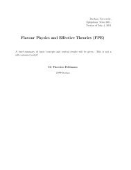
1.3. <strong>Higgs</strong> searches <strong>at</strong> colliders 17Figure 1.2: A sample <strong>Higgs</strong>strahlung diagram <strong>in</strong> which the <strong>Higgs</strong> <strong>boson</strong> is radi<strong>at</strong>edfrom a massive Z vector <strong>boson</strong>. S<strong>in</strong>ce the <strong>Higgs</strong>-electron coupl<strong>in</strong>g is small this wasthe dom<strong>in</strong>ant <strong>Higgs</strong> <strong>production</strong> mechanism <strong>at</strong> LEP.1.3 <strong>Higgs</strong> searches <strong>at</strong> collidersIn this section we describe the results <strong>of</strong> various searches for the <strong>Higgs</strong> <strong>boson</strong> <strong>at</strong>different colliders. We discuss the current lowest bound on the <strong>Higgs</strong> mass, whichcomes from LEP. We also discuss the exclusion region around 2m W observed by theTev<strong>at</strong>ron, and discuss search str<strong>at</strong>egies and potentials <strong>at</strong> the LHC.1.3.1 <strong>Higgs</strong> searches <strong>at</strong> LEPThe Large Electron-Positron (LEP) collider oper<strong>at</strong>ed <strong>at</strong> CERN between 1989 and2000, collid<strong>in</strong>g electrons and positrons <strong>with</strong> a centre <strong>of</strong> mass energy between 90 and209 GeV. Its <strong>Higgs</strong> searches focused primarily on direct <strong>production</strong> whilst precisionmeasurements <strong>of</strong> the W and Z mass allowed constra<strong>in</strong>ts to be placed on m H throughquantum effects. These <strong>in</strong>direct searches constra<strong>in</strong>ed m H < 193 GeV/c 2 <strong>at</strong> the 95%confidence level and favoured a mass <strong>in</strong> the range 81 +51−33 GeV/c 2 [48].Direct <strong>production</strong> <strong>of</strong> a <strong>Higgs</strong> <strong>boson</strong> <strong>at</strong> a lepton collider is made more difficult s<strong>in</strong>cethe collid<strong>in</strong>g particles have very small coupl<strong>in</strong>gs to the <strong>Higgs</strong> (s<strong>in</strong>ce the coupl<strong>in</strong>g isproportional to the mass <strong>of</strong> the particle). This means th<strong>at</strong> the dom<strong>in</strong>ant <strong>production</strong>mechanism <strong>of</strong> a <strong>Higgs</strong> <strong>boson</strong> <strong>at</strong> a lepton collider is through the <strong>Higgs</strong>strahlungprocess, (<strong>in</strong> which a <strong>Higgs</strong> is radi<strong>at</strong>ed from a Z <strong>boson</strong>) for which a sample diagramis shown <strong>in</strong> Fig. 1.2 [49,50]. For the range <strong>of</strong> <strong>Higgs</strong> <strong>boson</strong> masses which were relevantfor the LEP studies the <strong>Higgs</strong> predom<strong>in</strong><strong>at</strong>ely decayed to bb pairs (<strong>with</strong> a branch<strong>in</strong>g
1.3. <strong>Higgs</strong> searches <strong>at</strong> colliders 18r<strong>at</strong>io <strong>of</strong> 74%). The branch<strong>in</strong>g r<strong>at</strong>ios for the decays to τ + τ − , WW ∗ and gg are around7% <strong>with</strong> the rema<strong>in</strong><strong>in</strong>g ≈ 4% decay to cc.The f<strong>in</strong>al st<strong>at</strong>es which were <strong>in</strong>cluded <strong>in</strong> the f<strong>in</strong>al comb<strong>in</strong>ed analyses [51–55] werethe four-jet f<strong>in</strong>al st<strong>at</strong>e (H → bb)(Z → qq), the miss<strong>in</strong>g energy f<strong>in</strong>al st<strong>at</strong>e (H →bb)(Z → νν), the leptonic f<strong>in</strong>al st<strong>at</strong>e (H → bb)(Z → l + l − ) l ∈ {e, µ} and the taulepton f<strong>in</strong>al st<strong>at</strong>es, (H → bb)(Z → τ + τ − ) and (H → τ + τ − )(Z → qq). The result<strong>of</strong> the comb<strong>in</strong>ed direct searches, [51] was a limit on the lightest a SM <strong>Higgs</strong> <strong>boson</strong>could be. They found a lower bound <strong>of</strong> 114.4 GeV/c 2 <strong>at</strong> the 95% confidence level.Fig. 1.3 summarises these results.1.3.2 <strong>Higgs</strong> searches <strong>at</strong> the Tev<strong>at</strong>ron and the LHCThe <strong>two</strong> colliders currently search<strong>in</strong>g for the <strong>Higgs</strong> <strong>boson</strong>, Fermilab’s Tev<strong>at</strong>ron andCERN’s LHC are both hadronic colliders (the Tev<strong>at</strong>ron collides protons and antiprotons,the LHC collides protons). As such the ma<strong>in</strong> <strong>Higgs</strong> <strong>production</strong> mechanismsare completely different from those <strong>at</strong> LEP and are shown <strong>in</strong> Figs. 1.4-1.5, the largerenergy associ<strong>at</strong>ed <strong>with</strong> these colliders also <strong>in</strong>troduces new <strong>Higgs</strong> decay modes, whichare shown <strong>in</strong> Fig. 1.6.The dom<strong>in</strong>ant <strong>production</strong> mechanism <strong>at</strong> both colliders occurs through the gluonfusion process, which is the ma<strong>in</strong> topic <strong>of</strong> the next section. It is <strong>in</strong>terest<strong>in</strong>g tonote the differences between the subdom<strong>in</strong>ant <strong>production</strong> mechanisms between thecolliders. At the Tev<strong>at</strong>ron the second largest source <strong>of</strong> <strong>Higgs</strong> <strong>boson</strong>s occurs throughW and Z <strong>Higgs</strong>strahlung, the quark equivalent <strong>of</strong> the ma<strong>in</strong> process <strong>at</strong> LEP. However,<strong>at</strong> the LHC it is Vector-<strong>boson</strong> fusion (VBF or sometimes referred to as WBF) whichis the sub-dom<strong>in</strong>ant process. This is not merely due to the difference <strong>in</strong> centre <strong>of</strong>mass energies between the colliders, but due to the fact th<strong>at</strong> <strong>in</strong> an anti-proton thereare more valence anti-quarks than <strong>in</strong> a proton and as result processes <strong>in</strong> which quarkannihil<strong>at</strong>ion occur are favoured <strong>at</strong> the Tev<strong>at</strong>ron.We note th<strong>at</strong> <strong>in</strong> Fig. 1.6 there is a clear change <strong>in</strong> <strong>Higgs</strong> branch<strong>in</strong>g r<strong>at</strong>io aroundm H ≈ 130 GeV below these values the <strong>Higgs</strong> decays mostly <strong>in</strong>to bb pairs, whilst
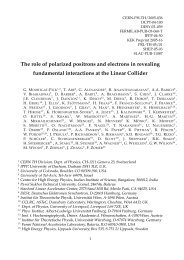
1.3. <strong>Higgs</strong> searches <strong>at</strong> colliders 19CL s110 -1LEP10 -210 -310 -4ObservedExpected forbackground10 -5114.4115.310 -6100 102 104 106 108 110 112 114 116 118 120m H(GeV/c 2 )Figure 1.3: Search results from the LEP collabor<strong>at</strong>ion [51], the solid l<strong>in</strong>e <strong>in</strong>dic<strong>at</strong>esobserv<strong>at</strong>ion, the dashed l<strong>in</strong>e <strong>in</strong>dic<strong>at</strong><strong>in</strong>g the median expect<strong>at</strong>ion for the background.The dark shaded bands <strong>in</strong>dic<strong>at</strong>e the 68% and 95% probability bands. The <strong>in</strong>tersection<strong>of</strong> the horizontal l<strong>in</strong>e for CL s = 0.05 <strong>with</strong> the observed curve is used to def<strong>in</strong>ethe 95% confidence lower bound on m H .
1.3. <strong>Higgs</strong> searches <strong>at</strong> colliders 20SM <strong>Higgs</strong> <strong>production</strong>10 3 100 120 140 160 180 200σ [fb]qq → WHgg → HTeV II10 2qq → qqH10bb → Hqq → ZH1gg,qq → ttHTeV4LHC <strong>Higgs</strong> work<strong>in</strong>g groupm H[GeV]Figure 1.4: <strong>Higgs</strong> <strong>production</strong> <strong>at</strong> the Tev<strong>at</strong>ron (taken from [56]), Run II <strong>of</strong> theTev<strong>at</strong>ron collides protons and anti-protons <strong>at</strong> a centre <strong>of</strong> mass energy <strong>of</strong> 1.96 TeV.The dom<strong>in</strong>ant <strong>production</strong> mechanism is gluon fusion. The second most dom<strong>in</strong>antmechanism is W <strong>Higgs</strong>strahlung, followed by Vector-<strong>boson</strong>-fusion (VBF).
1.3. <strong>Higgs</strong> searches <strong>at</strong> colliders 21σ [fb]10 4qq → qqHSM <strong>Higgs</strong> <strong>production</strong>gg → HLHC10 5 100 200 300 400 50010 3qq → WH10 2bb → Hqb → qtHTeV4LHC <strong>Higgs</strong> work<strong>in</strong>g groupgg,qq → ttHqq → ZHm H[GeV]Figure 1.5: <strong>Higgs</strong> <strong>production</strong> <strong>at</strong> the LHC (taken from [56]) for a design centre <strong>of</strong>mass energy <strong>of</strong> 14 TeV. In a similar fashion to the Tev<strong>at</strong>ron gluon fusion dom<strong>in</strong><strong>at</strong>esover all other channels, however, for the LHC VBF is now the subdom<strong>in</strong>ant channeland <strong>Higgs</strong>strahlung is suppressed.
1.3. <strong>Higgs</strong> searches <strong>at</strong> colliders 22m H[GeV]Figure 1.6: <strong>Higgs</strong> decay modes for an <strong>in</strong>terest<strong>in</strong>g range <strong>of</strong> <strong>Higgs</strong> masses [56,57]. Forlight <strong>Higgs</strong> <strong>boson</strong>s (m H 130 GeV) bb is the dom<strong>in</strong>ant decay mode. For all othermasses W + W − dom<strong>in</strong><strong>at</strong>es, for large masses tt becomes an important cannel.above these masses the <strong>Higgs</strong> decays preferentially <strong>in</strong>to W + W − . This l<strong>at</strong>ter channel<strong>with</strong> leptonic W decay is much cleaner <strong>at</strong> hadron colliders s<strong>in</strong>ce <strong>in</strong> an hadronicenvironment pick<strong>in</strong>g out QCD decays <strong>of</strong> the <strong>Higgs</strong> is extremely difficult due to thelarge irreducible backgrounds.The peak <strong>in</strong> the H → W + W − spectrum around m H ≈ 2m W gives a particularsensitivity to a <strong>Higgs</strong> <strong>boson</strong> <strong>in</strong> this mass range. Indeed the Tev<strong>at</strong>ron has recentlyproduced results [58] which exclude a <strong>Higgs</strong> <strong>boson</strong> <strong>in</strong> the mass range 162-166 GeV<strong>at</strong> the 95% CL. This is based on the comb<strong>in</strong>ed analysis [58] <strong>of</strong> 4.8 [59] (CDF) and5.4 [60] (D0) fb −1 d<strong>at</strong>a sets. The experiments <strong>in</strong>vestig<strong>at</strong>ed events <strong>with</strong> large miss<strong>in</strong>gtransverse energy and <strong>two</strong> oppositely charged leptons, target<strong>in</strong>g the H → W + W −signal, <strong>in</strong> which both Ws decay leptonically. The results are shown <strong>in</strong> Fig. 1.7.It should be noted th<strong>at</strong> <strong>in</strong> this analysis theoretical predictions for the <strong>Higgs</strong> crosssection play a crucial role, which we will talk more about <strong>in</strong> Chapter 6. Veryrecently, [61] the comb<strong>in</strong>ed CDF (5.9) fb −1 and D0 (6.7) fb −1 results have beenpublished, <strong>in</strong>creas<strong>in</strong>g the exclusion limits to 158 < m H < 175 GeV/c 2 , the resultsare summarised <strong>in</strong> Fig 1.8.
1.4. Effective coupl<strong>in</strong>g between gluons and a <strong>Higgs</strong> <strong>in</strong> the limit <strong>of</strong> aheavy top quark 23R lim10CDF + D0 Run IIL=4.8-5.4 fb -1ObservedExpectedExpected ±1σExpected ±2σ1SM=1130 140 150 160 170 180 190 200m H(GeV)Figure 1.7: Comb<strong>in</strong>ed CDF and D0 <strong>Higgs</strong> search results [58]. The sensitivity around2m W allows an exclusion region to develop around these masses. The exclusionoccurs where the observed l<strong>in</strong>e falls below the theoretical prediction.Over the next decade, as the LHC g<strong>at</strong>hers a large enough d<strong>at</strong>a set, the <strong>Higgs</strong><strong>boson</strong> will either be observed or excluded <strong>in</strong> the theoretically acceptable region.Like the Tev<strong>at</strong>ron, the LHC will be more sensitive to a heavy <strong>Higgs</strong> [62], howeverit should g<strong>at</strong>her a enough d<strong>at</strong>a to allow even very rare decays (but experimentallyfavourable) <strong>of</strong> light <strong>Higgs</strong> <strong>boson</strong>s such as H → γγ to be <strong>in</strong>vestig<strong>at</strong>ed.1.4 Effective coupl<strong>in</strong>g between gluons and a <strong>Higgs</strong><strong>in</strong> the limit <strong>of</strong> a heavy top quark1.4.1 Effective LagrangianIn this section we <strong>in</strong>troduce the effective Lagrangian which couples gluons to the<strong>Higgs</strong> <strong>boson</strong> [63–65]. S<strong>in</strong>ce the <strong>Higgs</strong> <strong>boson</strong> only couples to massive particles the<strong>in</strong>teraction proceeds predom<strong>in</strong>antly through a top quark loop. The dependence onthe top mass quickly makes calcul<strong>at</strong>ions extremely difficult, s<strong>in</strong>ce <strong>at</strong> LO <strong>in</strong> the full
1.4. Effective coupl<strong>in</strong>g between gluons and a <strong>Higgs</strong> <strong>in</strong> the limit <strong>of</strong> aheavy top quark 24Tev<strong>at</strong>ron Run II Prelim<strong>in</strong>ary, = 5.9 fb -195% CL Limit/SM101LEP ExclusionSM=1ExpectedObserved±1σ Expected±2σ ExpectedTev<strong>at</strong>ronExclusionTev<strong>at</strong>ron Exclusion July 19, 2010100 110 120 130 140 150 160 170 180 190 200m H(GeV/c 2 )Figure 1.8: Comb<strong>in</strong>ed CDF and D0 results [61], the <strong>in</strong>creased d<strong>at</strong>a set (rel<strong>at</strong>iveto [58]) has <strong>in</strong>creased the exclusion limit around 2m W . The results are also beg<strong>in</strong>n<strong>in</strong>gto approach the LEP lower limit on the <strong>Higgs</strong> mass.Figure 1.9: The <strong>Higgs</strong>-gluon coupl<strong>in</strong>g <strong>in</strong> the Standard Model proceeds through <strong>at</strong>op quark loop, <strong>at</strong> LO order <strong>in</strong> the full theory this is the only contribut<strong>in</strong>g diagram.
1.4. Effective coupl<strong>in</strong>g between gluons and a <strong>Higgs</strong> <strong>in</strong> the limit <strong>of</strong> aheavy top quark 25theory one must deal <strong>with</strong> massive loops and massive external particles. Amplitudes<strong>with</strong> a <strong>Higgs</strong> <strong>boson</strong> and up to four gluons have been calcul<strong>at</strong>ed <strong>at</strong> LO <strong>in</strong> the fulltheory [66–68]. Processes which allow large amounts <strong>of</strong> colour annihil<strong>at</strong>ion typicallyhave large K factors, and as such we expect NLO contributions to gluon fusion tobe large. S<strong>in</strong>ce NLO calcul<strong>at</strong>ions <strong>in</strong> the full theory <strong>in</strong>volve <strong>two</strong> loop diagrams <strong>with</strong>a massive loop, these calcul<strong>at</strong>ions are formidable. To simplify the problem we canwork <strong>in</strong> an effective theory <strong>in</strong> which the top mass is sent to <strong>in</strong>f<strong>in</strong>ity [63–65]. Thisapproxim<strong>at</strong>ion will work well provided th<strong>at</strong> m H < 2m t . In this effective theory thetop loops are <strong>in</strong>tegr<strong>at</strong>ed out to produce vertices. These vertices arise from higherdimensionalterms <strong>in</strong> the Lagrangian which directly couple <strong>Higgs</strong> <strong>boson</strong>s and gluonfield strengths. The first <strong>of</strong> these terms is five dimensional, successive terms, whichare higher dimensional, conta<strong>in</strong> higher powers <strong>of</strong> gluon field strengths,L <strong>in</strong>teff = 1 2 CH trGµν G µν + C ′ H trG µ ν Gν ρ Gρ µ + . . .. (1.49)S<strong>in</strong>ce each term <strong>in</strong> the Lagrangian is ultim<strong>at</strong>ely four dimensional we observe th<strong>at</strong>C ′ ∼ C/m 2 t, i.e. each <strong>of</strong> the higher dimensional Lagrangian pieces are suppressedby powers <strong>of</strong> m t . Therefore <strong>in</strong> the m t → ∞ limit only the first term contributes to<strong>Higgs</strong> plus gluon amplitudes. O(m 2 H /m2 t ) corrections can be <strong>in</strong>cluded by calcul<strong>at</strong><strong>in</strong>gamplitudes us<strong>in</strong>g the higher-dimensional pieces <strong>of</strong> the Lagrangian. One can use thesehigher-dimensional effective oper<strong>at</strong>ors to calcul<strong>at</strong>e O(1/m 2 t ) corrections to <strong>Higgs</strong> plusjet amplitudes <strong>in</strong> the effective theory [69].To make predictions us<strong>in</strong>g the effective theory Lagrangian we must obta<strong>in</strong> theWilson coefficient C, this can be done by m<strong>at</strong>ch<strong>in</strong>g to fixed order calcul<strong>at</strong>ions <strong>in</strong> thefull theory. In this way one obta<strong>in</strong>s C as a perturb<strong>at</strong>ion series <strong>in</strong> α S , for example<strong>at</strong> lead<strong>in</strong>g order the (colour stripped) m<strong>at</strong>rix element for H → gg <strong>in</strong> the effectivetheory is,M Eff (H → gg) = −iCg µν p 1 · p 2 ǫ ∗µ1 ǫ ∗ν2 (1.50)where p i and ǫ ∗ i represent the momentum and polaris<strong>at</strong>ion vector <strong>of</strong> gluon i. Wecan also calcul<strong>at</strong>e the H → gg amplitude <strong>in</strong> the full theory,where there is only onediagram, the triangle diagram shown <strong>in</strong> Fig 1.9. In the m t → ∞ limit the m<strong>at</strong>rix
1.4. Effective coupl<strong>in</strong>g between gluons and a <strong>Higgs</strong> <strong>in</strong> the limit <strong>of</strong> aheavy top quark 26element takes the follow<strong>in</strong>g form,M FTm t→∞ (H → gg) = −i α s6πv g µνp 1 · p 2 ǫ ∗µ1 ǫ∗ν 2 + . . . (1.51)where . . . represent pieces which are suppressed <strong>in</strong> the large top limit. We candeterm<strong>in</strong>e the coefficient C by m<strong>at</strong>ch<strong>in</strong>g eq. (1.50) and eq. (1.51).C α S= α S6πv(1.52)To compute C to higher orders <strong>in</strong> α S one must calcul<strong>at</strong>e M FTm t→∞(H → gg) <strong>at</strong>higher loops, The effective coupl<strong>in</strong>g C has been calcul<strong>at</strong>ed up to order O(αs 3 ) <strong>in</strong> [70].However, for our purposes we need it only up to order O(αs) 2 [71],(αC α2 sS = 1 + 11 )6πv 4π α s + O(αs 3 ) (1.53)One can also def<strong>in</strong>e the follow<strong>in</strong>g quantity R which is given by the r<strong>at</strong>ioR =σ(H → gg)σ mt→∞(H → gg) , (1.54)where σ(gg → H) is the total cross section. Sett<strong>in</strong>g x = 4m 2 t /m2 Hthe correction forthe f<strong>in</strong>ite mass <strong>of</strong> the top quark <strong>in</strong> the region x > 1 is [72],[3x( [R = 1 − (x − 1) s<strong>in</strong> −1 1] 2 ) ] 2√x . (1.55)2This quantity when used to normalise an effective theory cross section providesa good approxim<strong>at</strong>ion <strong>of</strong> the cross section from the full theory, see Ref. [66] andreferences there<strong>in</strong>.It has been known for a long time th<strong>at</strong> the radi<strong>at</strong>ive corrections to <strong>Higgs</strong> <strong>production</strong>through gluon fusion are large [72–74]. These NLO studies showed th<strong>at</strong>go<strong>in</strong>g beyond NLO was essential and impressively fully differential cross-sections<strong>at</strong> NNLO have now been calcul<strong>at</strong>ed [75–82]. Recent calcul<strong>at</strong>ions have studied theeffect <strong>of</strong> f<strong>in</strong>ite top masses on the NNLO calcul<strong>at</strong>ions [83–88]. They found themto be reasonably small, <strong>in</strong>dic<strong>at</strong><strong>in</strong>g th<strong>at</strong> for <strong>Higgs</strong> <strong>production</strong> through gluon fusionthe effective theory works well. The NNLO results can also be improved by <strong>in</strong>clud<strong>in</strong>gnext-to-next-to-lead<strong>in</strong>g logarithmic (NNLL) s<strong>of</strong>t gluon resumm<strong>at</strong>ion [89] 5 .5 At the Tev<strong>at</strong>ron this results <strong>in</strong> an <strong>in</strong>crease <strong>in</strong> cross section <strong>of</strong> around 13%.
1.4. Effective coupl<strong>in</strong>g between gluons and a <strong>Higgs</strong> <strong>in</strong> the limit <strong>of</strong> aheavy top quark 27These calcul<strong>at</strong>ions have been confirmed by calcul<strong>at</strong>ion <strong>of</strong> s<strong>of</strong>t terms to N 3 LO accuracy[90,91].When more partons are considered <strong>in</strong> the f<strong>in</strong>al st<strong>at</strong>e top mass effects becomemore pronounced. It has been shown th<strong>at</strong> top and bottom quark mass effects canplay an important role [92] <strong>in</strong> devi<strong>at</strong>ions from the effective theory results [93,94] for<strong>Higgs</strong> plus jet calcul<strong>at</strong>ions <strong>at</strong> NLO. We discuss the role <strong>of</strong> additional <strong>jets</strong> further(<strong>with</strong> an emphasis on <strong>two</strong> <strong>jets</strong>) <strong>in</strong> section 1.5.1.4.2 φ, φ † splitt<strong>in</strong>g <strong>of</strong> the Effective LagrangianWhen we look <strong>at</strong> a simple <strong>Higgs</strong> plus gluon helicity amplitude <strong>at</strong> tree-level a h<strong>in</strong>t <strong>of</strong>structure jumps out <strong>at</strong> us,A (0)4 (φ, 1 − , 2 + , 3 − , 4 + ) =〈13〉 4〈12〉〈23〉〈34〉〈41〉 + [24] 4[12][23][34][41] . (1.56)Here we have used the sp<strong>in</strong>or helicity formalism, which is described <strong>in</strong> Appendix A.Eq. (1.56) has a clear structure, if momentum were conserved amongst the gluons(p H → 0) then the <strong>two</strong> terms would be conjug<strong>at</strong>es <strong>of</strong> each other. With this <strong>in</strong> m<strong>in</strong>dwe make the follow<strong>in</strong>g def<strong>in</strong>itions, [95],φ =(H + iA), φ † =2(H − iA). (1.57)2Here A is a massive pseudo-scalar. We also wish to divide the gluon field strengthtensor G µν <strong>in</strong>to self-dual (SD) and anti-self dual (ASD) pieces,G µνSD = 1 2 (Gµν + ∗ G µν ) G µνASD = 1 2 (Gµν − ∗ G µν ), (1.58)<strong>with</strong>∗ G µν = i 2 ǫµνρσ G ρσ . (1.59)In terms <strong>of</strong> these def<strong>in</strong>itions the Lagrangian takes the follow<strong>in</strong>g form,][HtrG µν G µν + iAtrG ∗ µνG µνL <strong>in</strong>tH,A = C 2= C[]φtrG SD µν G µ,νSD + φ† trG ASD µν G µ,νASD. (1.60)
1.5. <strong>Higgs</strong> plus <strong>two</strong> <strong>jets</strong>: Its phenomenological role and an overview <strong>of</strong>this thesis 28The effective <strong>in</strong>teraction l<strong>in</strong>k<strong>in</strong>g gluons and scalar fields splits <strong>in</strong>to a piece conta<strong>in</strong><strong>in</strong>gφ and the self-dual gluon field strengths and another part l<strong>in</strong>k<strong>in</strong>g φ † to the anti-selfdualgluon field strengths. The last step conveniently embeds the <strong>Higgs</strong> <strong>in</strong>teraction<strong>with</strong><strong>in</strong> the MHV structure <strong>of</strong> the QCD amplitudes. The self-duality <strong>of</strong> φ amplitudesalso results <strong>in</strong> them hav<strong>in</strong>g a simpler structure than <strong>Higgs</strong> amplitudes. The full<strong>Higgs</strong> amplitudes are then written as a sum <strong>of</strong> the φ (self-dual) and φ † (anti-selfdual)components,A (l)n (H; {p k }) = A (l)n (φ, {p k }) + A (l)n (φ † , {p k }). (1.61)We can also gener<strong>at</strong>e pseudo-scalar amplitudes from the difference <strong>of</strong> φ and φ †components,A n (l) (A; {p k }) = 1 (A(l)n (φ, {p k }) − A n (l) (φ † , {p k }) ) . (1.62)iFurthermore parity rel<strong>at</strong>es φ and φ † amplitudes,(∗A n (m) (φ† , g λ 11 , . . .,gλn n ) = A n (m) (φ, g−λ 11 , . . ., gn )) −λn . (1.63)From now on, we will only consider φ-amplitudes, know<strong>in</strong>g th<strong>at</strong> all others can beobta<strong>in</strong>ed us<strong>in</strong>g eqs. (1.61)–(1.63). We will discuss tree amplitudes conta<strong>in</strong><strong>in</strong>g a φand partons <strong>in</strong> Appendix A.1.5 <strong>Higgs</strong> plus <strong>two</strong> <strong>jets</strong>: Its phenomenological roleand an overview <strong>of</strong> this thesisAs has been mentioned earlier <strong>in</strong> the chapter, an important search channel for the<strong>Higgs</strong> <strong>boson</strong>, <strong>in</strong> the mass range 115 < m H < 160 GeV, is <strong>production</strong> via weak <strong>boson</strong>fusion [96]. A <strong>Higgs</strong> <strong>boson</strong> produced <strong>in</strong> this channel is expected to be producedrel<strong>at</strong>ively centrally, <strong>in</strong> <strong>associ<strong>at</strong>ion</strong> <strong>with</strong> <strong>two</strong> hard forward <strong>jets</strong>. These strik<strong>in</strong>g k<strong>in</strong>em<strong>at</strong>icfe<strong>at</strong>ures are expected to enable a search for such events despite the otherwiseoverwhelm<strong>in</strong>g QCD backgrounds. Confidence <strong>in</strong> the theoretical prediction for the<strong>Higgs</strong> signal process is based upon knowledge <strong>of</strong> next-to-lead<strong>in</strong>g order corrections <strong>in</strong>both QCD [97–99] and <strong>in</strong> the electroweak sector [100,101].
1.5. <strong>Higgs</strong> plus <strong>two</strong> <strong>jets</strong>: Its phenomenological role and an overview <strong>of</strong>this thesis 29However, <strong>in</strong> addition to the weak process, a significant number <strong>of</strong> such eventsmay also be produced via the strong <strong>in</strong>teraction. In order to accur<strong>at</strong>ely predictthe signal and, <strong>in</strong> particular, to simul<strong>at</strong>e faithfully the expected significance <strong>in</strong> agiven <strong>Higgs</strong> model, a fully differential NLO calcul<strong>at</strong>ion <strong>of</strong> QCD <strong>production</strong> <strong>of</strong> a<strong>Higgs</strong> and <strong>two</strong> hard <strong>jets</strong> is also required. The <strong>in</strong>terference between the weak <strong>boson</strong>fusion process and gluon fusion have been calcul<strong>at</strong>ed and shown to be experimentallynegligible [102].In the Standard Model the <strong>Higgs</strong> couples to <strong>two</strong> gluons via a top-quark loop.Calcul<strong>at</strong>ions which <strong>in</strong>volve the full dependence on m t are difficult and a drasticsimplific<strong>at</strong>ion can be achieved if one works <strong>in</strong> an effective theory <strong>in</strong> which the mass <strong>of</strong>the top quark is large [65,72,73]. For <strong>in</strong>clusive <strong>Higgs</strong> <strong>production</strong> this approxim<strong>at</strong>ionis valid over a wide range <strong>of</strong> <strong>Higgs</strong> masses and, for processes <strong>with</strong> additional <strong>jets</strong>,the approxim<strong>at</strong>ion is justified provided th<strong>at</strong> the transverse momentum <strong>of</strong> each jetis smaller than m t [67]. Tree-level calcul<strong>at</strong>ions have been performed <strong>in</strong> both thelarge-m t limit [64,103] and <strong>with</strong> the exact-m t [67] dependence.Results for the one-loop corrections to all <strong>of</strong> the <strong>Higgs</strong> + 4 parton processes havebeen published <strong>in</strong> 2005 [104]. Although analytic results were provided for the <strong>Higgs</strong>¯qq¯qq processes, the bulk <strong>of</strong> this calcul<strong>at</strong>ion was performed us<strong>in</strong>g a semi-numericalmethod. In this approach the loop <strong>in</strong>tegrals were calcul<strong>at</strong>ed analytically whereasthe coefficients <strong>with</strong> which they appear <strong>in</strong> the loop amplitudes were computed numericallyus<strong>in</strong>g a recursive method. Although some phenomenology was performedus<strong>in</strong>g this calcul<strong>at</strong>ion [105], the implement<strong>at</strong>ion <strong>of</strong> fully analytic formulae will leadto a faster code and permit more extensive phenomenological <strong>in</strong>vestig<strong>at</strong>ions, whichis the ma<strong>in</strong> goal <strong>of</strong> this thesis.S<strong>in</strong>ce then there has been a drive to produce analytic results for the process,<strong>with</strong> the aim <strong>of</strong> improv<strong>in</strong>g the speed <strong>of</strong> the calcul<strong>at</strong>ion. This thesis conta<strong>in</strong>s calcul<strong>at</strong>ionsfor the most complic<strong>at</strong>ed helicity configur<strong>at</strong>ions; the φ-NMHV helicityconfigur<strong>at</strong>ions (both the pure gluon and qqgg cases), and the non-adjacent MHVhelicity gluon configur<strong>at</strong>ion. The rema<strong>in</strong><strong>in</strong>g calcul<strong>at</strong>ions have been performed elsewhere;the r<strong>at</strong>ional amplitudes (φ + + + +), (φ, − + ++) and (φ, qq + +) have
1.5. <strong>Higgs</strong> plus <strong>two</strong> <strong>jets</strong>: Its phenomenological role and an overview <strong>of</strong>this thesis 30been performed <strong>in</strong> [106] the all m<strong>in</strong>us and adjacent m<strong>in</strong>us MHV case can be found<strong>in</strong> [107,108], whilst the φqq-MHV amplitudes (as well as φqqQQ helicity amplitudes)can be found <strong>in</strong> [109].This thesis proceeds as follows, <strong>in</strong> chapter 2 we present an overview <strong>of</strong> the on-shelltechniques which we will use throughout the thesis. Chapter 3 conta<strong>in</strong>s the calcul<strong>at</strong>ion<strong>of</strong> the φ MHV amplitude <strong>with</strong> general helicites, we present the cut-constructiblepieces for all multiplicities, whilst for the r<strong>at</strong>ional pieces we focus on the four-gluonamplitude we are ultim<strong>at</strong>ely <strong>in</strong>terested <strong>in</strong>. Chapter 4 describes the calcul<strong>at</strong>ion <strong>of</strong>the φ-NMHV and summarises the results for the four gluon amplitudes. The lastchapter deal<strong>in</strong>g <strong>with</strong> analytic calcul<strong>at</strong>ions is chapter 5, which presents the rema<strong>in</strong><strong>in</strong>ghelicity amplitude, the φqq-NMHV amplitude. Chapter 6 then moves from analyticcalcul<strong>at</strong>ions <strong>in</strong>to describ<strong>in</strong>g some phenomenology which can be performed <strong>with</strong> thenew results. In chapter 7 we draw our conclusions. Appendix A conta<strong>in</strong>s a review<strong>of</strong> both the sp<strong>in</strong>or helicity formalism and colour order<strong>in</strong>g <strong>of</strong> tree and one-loop amplitudesas well as a list <strong>of</strong> useful tree amplitudes. Appendix B conta<strong>in</strong>s explicitformulae for the basis <strong>in</strong>tegrals we use <strong>in</strong> this work.
Chapter 2Unitarity and on-shell methods2.1 UnitarityInspired by the optical theorem, unitarity techniques have recently become widelyused <strong>in</strong> the calcul<strong>at</strong>ion <strong>of</strong> one-loop multi-particle amplitudes. These techniques,orig<strong>in</strong>ally pioneered by Bern, Dixon, Dunbar and Kosower <strong>in</strong> the mid-90’s [110,111],have been revolutionised over the last few years by the <strong>in</strong>troduction <strong>of</strong> complexmomenta and generalised unitarity.In this section we will outl<strong>in</strong>e the ma<strong>in</strong> pr<strong>in</strong>ciples <strong>of</strong> generalised unitarity. In a broadsense these methods can be classified as either four or D-dimensional techniques,both <strong>of</strong> which are <strong>in</strong>troduced <strong>in</strong> the follow<strong>in</strong>g sections. We will also discuss on-shelltechniques for the gener<strong>at</strong>ion <strong>of</strong> tree-level amplitudes, the MHV rules and BCFWrecursion rel<strong>at</strong>ions. The unitarity-boostrap, a fully four-dimensional method forgener<strong>at</strong><strong>in</strong>g one-loop amplitudes, is also <strong>in</strong>troduced. F<strong>in</strong>ally we review the recentprogress towards one-loop automis<strong>at</strong>ion.2.1.1 Unitarity: An IntroductionAt the heart <strong>of</strong> unitarity methods lies the optical theorem, which rel<strong>at</strong>es the discont<strong>in</strong>uity<strong>of</strong> a m<strong>at</strong>rix element to its imag<strong>in</strong>ary part. When expanded <strong>in</strong> a perturb<strong>at</strong>ionseries <strong>in</strong> the relevant coupl<strong>in</strong>g constant the first non-trivial result rel<strong>at</strong>es the product31
2.1. Unitarity 32<strong>of</strong> <strong>two</strong> tree level amplitudes to the discont<strong>in</strong>uity <strong>of</strong> a one-loop <strong>in</strong>tegral function. Thediscont<strong>in</strong>uity <strong>of</strong> a one-loop <strong>in</strong>tegral associ<strong>at</strong>ed <strong>with</strong> a k<strong>in</strong>em<strong>at</strong>ic scale s = P 2 can bedeterm<strong>in</strong>ed by replac<strong>in</strong>g (or cutt<strong>in</strong>g) the follow<strong>in</strong>g propag<strong>at</strong>ors,1l 2 + iǫ → −2πiδ(l2 ),1(l + P) 2 + iǫ → −2πiδ((l + P)2 ). (2.1)In the mid-90’s Bern, Dixon, Dunbar and Kosower used these rel<strong>at</strong>ions to calcul<strong>at</strong>ea series <strong>of</strong> one-loop amplitudes [110,111]. The method <strong>in</strong>volves tak<strong>in</strong>g a cut <strong>in</strong> acerta<strong>in</strong> k<strong>in</strong>em<strong>at</strong>ic scale and then us<strong>in</strong>g the simplify<strong>in</strong>g k<strong>in</strong>em<strong>at</strong>ics <strong>of</strong> the cut (e.g. afour dimensional on-shell loop momenta) to reduce the complexity <strong>of</strong> the coefficients<strong>of</strong> the cut loop functions. The cut propag<strong>at</strong>ors are then re<strong>in</strong>st<strong>at</strong>ed so th<strong>at</strong> the <strong>in</strong>tegrandreturns to be<strong>in</strong>g a one-loop <strong>in</strong>tegral. This approach successfully determ<strong>in</strong>esthe coefficients <strong>of</strong> all basis <strong>in</strong>tegrals which conta<strong>in</strong> a cut <strong>in</strong> the k<strong>in</strong>em<strong>at</strong>ic scale. Integralswhich do not conta<strong>in</strong> a cut propag<strong>at</strong>or, but can arise <strong>in</strong> the reduction process,must be dropped and recovered <strong>in</strong> the appropri<strong>at</strong>e cuts.A major simplific<strong>at</strong>ion occurs when four-dimensional tree amplitudes are used<strong>in</strong> the cuts. This is because one can use the sp<strong>in</strong>or helicity formalism (which isdescribed <strong>in</strong> Appendix A) to produce compact helicity amplitudes. However, theprice <strong>of</strong> us<strong>in</strong>g four-dimensional cuts is the <strong>in</strong>ability to determ<strong>in</strong>e pieces <strong>of</strong> the amplitudewhich do not conta<strong>in</strong> discont<strong>in</strong>uities <strong>in</strong> the k<strong>in</strong>em<strong>at</strong>ic <strong>in</strong>variants. These pieces,lack<strong>in</strong>g such discont<strong>in</strong>uities, are referred to as the r<strong>at</strong>ional pieces [110,111]. Theirorig<strong>in</strong>, and elusiveness <strong>in</strong> four-dimensions can be thought <strong>of</strong> as follows, a generalterm <strong>in</strong> a one-loop amplitude has the follow<strong>in</strong>g structure,(C i · I i = (c 0 + c 1 ǫ + c 2 ǫ 2 I−2+ . . .) ·ǫ + I )−1+ I 2 0 · log({s, t, . . . }) + . . . . (2.2)ǫHere C i · I i represents a basis <strong>in</strong>tegral I i <strong>with</strong> a coefficient C i . In general I i canconta<strong>in</strong> poles <strong>of</strong> up to second order <strong>in</strong> the dimensionally regul<strong>at</strong><strong>in</strong>g parameter ǫ.The term log({s, t, . . . }) represents a generic piece <strong>of</strong> the <strong>in</strong>tegral which conta<strong>in</strong>slogarithms (these could also be di-logarithms or ln 2 ). It is these pieces which conta<strong>in</strong>a discont<strong>in</strong>uity <strong>in</strong> a k<strong>in</strong>em<strong>at</strong>ic <strong>in</strong>variant and hence enter the optical theorem.However when one uses four-dimensional trees, one loses all sensitivity to the higherorder pieces <strong>in</strong> ǫ which enter the coefficient multiply<strong>in</strong>g the discont<strong>in</strong>uity. Hence,
2.1. Unitarity 33four dimensional cuts are only sensitive to terms <strong>of</strong> the form c 0 I 0 . The miss<strong>in</strong>gpieces, which are <strong>of</strong> higher order <strong>in</strong> ǫ <strong>in</strong> the coefficient contribute f<strong>in</strong>ite pieces whenmultiply<strong>in</strong>g the pole pieces <strong>of</strong> the <strong>in</strong>tegral. This is why they can be thought <strong>of</strong> ashav<strong>in</strong>g no discont<strong>in</strong>uities <strong>in</strong> the k<strong>in</strong>em<strong>at</strong>ic <strong>in</strong>variants (but can still be detected byD-dimensional cuts).The separ<strong>at</strong>ion <strong>in</strong>to r<strong>at</strong>ional and cut-constructible pieces leads to divide andconquer str<strong>at</strong>egies for methods which rely on four-dimensional cuts. Unitarity techniquescan be used to calcul<strong>at</strong>e the cut-constructible pieces leav<strong>in</strong>g the r<strong>at</strong>ionalpieces to be determ<strong>in</strong>ed by some other method. For amplitudes <strong>in</strong> N = 4 andN = 1 supersymmetric Yang-Mills (SYM) theories, no additional methods areneeded, s<strong>in</strong>ce these amplitudes are completely determ<strong>in</strong>ed by their four-dimensionalcuts [110,111]. This realis<strong>at</strong>ion has led to many calcul<strong>at</strong>ions <strong>of</strong> amplitudes <strong>in</strong> thesetheories [110–116]. In addition to be<strong>in</strong>g <strong>in</strong>terest<strong>in</strong>g <strong>in</strong> their own right, these amplitudescan be used to construct gluonic amplitudes. If one comb<strong>in</strong>es one N = 4multiplet (which conta<strong>in</strong>s one gluon four fermions and three complex scalars), <strong>with</strong>four N = 1 chiral multiplets (each one conta<strong>in</strong><strong>in</strong>g one fermion and one complexscalar) one f<strong>in</strong>ds th<strong>at</strong>A gluonn = A N=4n − 4A N=1n + An N=0,scalar(2.3)Here the gluon loop is represented <strong>in</strong> terms <strong>of</strong> <strong>two</strong> pieces which are cut-constructibleand one piece which conta<strong>in</strong>s a complex scalar. This last piece, although not cutconstructible<strong>in</strong> four-dimensions, is simpler than the <strong>in</strong>itial gluon loop. Importantly,the r<strong>at</strong>ional pieces can be thought <strong>of</strong> aris<strong>in</strong>g from diagrams which conta<strong>in</strong> scalars,r<strong>at</strong>her than gluons, circul<strong>at</strong><strong>in</strong>g around the loop. The piece <strong>of</strong> gluon amplitudes whicharises from a fermion loop (and is proportional to the number <strong>of</strong> light flavours N F )has a similar breakdown.A gluon,N Fn = A N=1n − An N=0,scalar(2.4)So th<strong>at</strong> the r<strong>at</strong>ional parts <strong>of</strong> pure gluonic amplitudes are always proportional to(1 − N F /N C ) (which will be useful <strong>in</strong> l<strong>at</strong>er chapters).The unitarity method as described above (<strong>with</strong> various techniques to determ<strong>in</strong>e
2.2. Quadruple cuts 34the r<strong>at</strong>ional part) was used to calcul<strong>at</strong>e several phenomenologically important processes[117–119]. The ma<strong>in</strong> drawback <strong>of</strong> the method be<strong>in</strong>g th<strong>at</strong> for a given cut onewould f<strong>in</strong>d multiple basis <strong>in</strong>tegrals (for example a cut could conta<strong>in</strong> box, triangle andbubble contributions and all can enter simultaneously) and the appearance <strong>of</strong> terms<strong>in</strong> the reduction <strong>of</strong> tensors which do not conta<strong>in</strong> the appropri<strong>at</strong>e cut propag<strong>at</strong>ors.In 2004 unitarity methods were re<strong>in</strong>vigor<strong>at</strong>ed by several developments <strong>in</strong> onshelltechniques. New methods for gener<strong>at</strong><strong>in</strong>g compact helicity expressions werediscovered, the BCFW recursion rel<strong>at</strong>ions, and the MHV rules. At the same timethe idea <strong>of</strong> us<strong>in</strong>g multiple cuts was established as a useful technique, known asgeneralised unitarity.2.2 Quadruple cuts2.2.1 The quadruple cut methodAs discussed previously, massless one-loop amplitudes can be written <strong>in</strong> the follow<strong>in</strong>gbasis,A (1)n= ∑ i(c 4;i I 4,i + c 3;i I 3;i + c 2;i I 2;i ) + R n , (2.5)where I i;j is a basis <strong>in</strong>tegral <strong>with</strong> i propag<strong>at</strong>ors <strong>with</strong> a topology denoted by j (<strong>in</strong>the above equ<strong>at</strong>ion the summ<strong>at</strong>ion is over the various allowed topologies given theexternal momenta). S<strong>in</strong>ce the basis is process <strong>in</strong>dependent, the calcul<strong>at</strong>ion <strong>of</strong> oneloopamplitudes is essentially reduced to extract<strong>in</strong>g the coefficients <strong>of</strong> each basis<strong>in</strong>tegral as efficiently as possible. With this <strong>in</strong> m<strong>in</strong>d it was proposed [120] th<strong>at</strong> onecould isol<strong>at</strong>e a given box coefficient by apply<strong>in</strong>g four (r<strong>at</strong>her than <strong>two</strong>) cuts. S<strong>in</strong>ceonly the box terms <strong>in</strong> eq. (2.5) conta<strong>in</strong> four propag<strong>at</strong>ors each four-cut should isol<strong>at</strong>ean <strong>in</strong>dividual box,∫d 4 l4∏i=1δ(l 2 i)A (0)1 (l 1 , l 2 )A (0)2 (l 2 , l 3 )A (0)3 (l 3 , l 4 )A (0)4 (l 4 , l 1 )= c 4,{P }∫d 4 l4∏δ(l 2 i) (2.6)i=1
2.2. Quadruple cuts 35Here the LHS <strong>of</strong> eq. (2.6) represents the applic<strong>at</strong>ion <strong>of</strong> the four on-shell constra<strong>in</strong>tsδ(l 2 i ) to the LHS <strong>of</strong> eq. (2.5), shown schem<strong>at</strong>ically <strong>in</strong> Fig. 2.1, whilst the RHSrepresents the applic<strong>at</strong>ion <strong>of</strong> the four cuts to the basis <strong>in</strong>tegral. In four-dimensionsthe loop momenta has the same number <strong>of</strong> components as there are cut propag<strong>at</strong>orsand as such is frozen by the cuts. S<strong>in</strong>ce the <strong>in</strong>tegral over the cut phase space merelycontributes a Jacobian, which is identical on both sides <strong>of</strong> the equ<strong>at</strong>ion, we canrel<strong>at</strong>e the coefficient <strong>of</strong> a box (<strong>with</strong> a given topology P) to the solution <strong>of</strong> the fourproducts <strong>of</strong> treesA (0)1 (l 1 , l 2 )A (0)2 (l 2 , l 3 )A (0)3 (l 3 , l 4 )A (0)4 (l 4 , l 1 ) = c 4,{P } , (2.7)where the loop momenta are solved via the on-shell constra<strong>in</strong>ts.There is a subtlety, however, regard<strong>in</strong>g the applic<strong>at</strong>ion <strong>of</strong> four cuts to a one-loopamplitude. There are six classes <strong>of</strong> box <strong>in</strong>tegral which can be classified <strong>in</strong> terms <strong>of</strong>the number <strong>of</strong> legs bunched <strong>at</strong> each corner. Two or more legs <strong>at</strong> a specific cornerresults <strong>in</strong> a “mass” s<strong>in</strong>ce the squared sum <strong>of</strong> corner momenta is no longer zero. Forfour external (massless) particles it is thus possible to have a zero-mass box. As thenumber <strong>of</strong> external particles <strong>in</strong>crease so can the number <strong>of</strong> masses, one can drawa one-mass box, <strong>two</strong> <strong>two</strong>-mass boxes 1 , a three-mass and a four-mass box. For allbut the the four-mass box, after the applic<strong>at</strong>ion <strong>of</strong> the four-cut, one f<strong>in</strong>ds a cornerconta<strong>in</strong><strong>in</strong>g a three-po<strong>in</strong>t vertex A (0)3 (1λ 1, 2 λ 2, 3 λ 3). S<strong>in</strong>ce this amplitude is Lorentz<strong>in</strong>variant it must depend only on squares <strong>of</strong> the <strong>in</strong>dividual momenta p 2 i, or <strong>in</strong>variantproducts between them p i · p j . For massless momenta p 2 i = 0 so the amplitudecan only depend on <strong>in</strong>variant products between momenta. However, conserv<strong>at</strong>ion <strong>of</strong>momenta forces each product to be zero,(p i + p j ) 2 = p 2 k = 0 =⇒ p i · p j = 0, (2.8)which implies A (0)3 (1 λ 1, 2 λ 2, 3 λ 3) = 0. For real momenta this appears to be a majorflaw <strong>in</strong> the quadruple cut approach. The crucial observ<strong>at</strong>ion <strong>in</strong> [120] is th<strong>at</strong> ifone switches to complex momenta this obstacle can be overcome. Specifically, <strong>in</strong>1 The <strong>in</strong>tegral <strong>in</strong> which the massive corners are opposite is called the easy configur<strong>at</strong>ion. Theother configur<strong>at</strong>ion <strong>in</strong> which the masses are adjacent is referred to as the hard configur<strong>at</strong>ion
2.2. Quadruple cuts 360000000111111100000001111111000000011111110000000111111100000001111111000000011111110000000111111100000001111111000000011111110000000111111100000001111111000000011111110000000111111100000001111111000000011111110000000111111100000001111111000000011111110000000111111100000001111111000000011111110000000111111100000001111111000000011111110000000111111100000001111111000000011111110000000111111100000001111111000000011111110000000111111100000001111111000000011111110000000111111100000001111111000000011111110000000111111100000001111111000000011111110000000111111100000001111111000000011111110000000111111100000001111111Figure 2.1: The applic<strong>at</strong>ion <strong>of</strong> four cuts to a one-loop amplitude results <strong>in</strong> thefactoris<strong>at</strong>ion onto the product <strong>of</strong> four tree amplitudes. S<strong>in</strong>ce boxes are the onlyone-loop basis function to conta<strong>in</strong> four propag<strong>at</strong>ors each four cut selects a uniquebox function from the basis. In addition for four-dimensional cuts the loop momentais frozen by the cutt<strong>in</strong>g procedure.
2.2. Quadruple cuts 37M<strong>in</strong>kowskii space (+ − −−) a bisp<strong>in</strong>or (light-like four vector) has the form p aȧ =λ a˜λȧ. For real momenta λ and ˜λ are complex but are rel<strong>at</strong>ed to each other, ˜λ = ±λ.This means th<strong>at</strong> when an <strong>in</strong>variant p i · p j = 0 both 〈ij〉 and [ij] equal zero (s<strong>in</strong>cethey are conjug<strong>at</strong>es <strong>of</strong> each other). If however, one drops the reality condition, suchth<strong>at</strong> λ and ˜λ are <strong>in</strong>dependent, one can still s<strong>at</strong>isfy momenta conserv<strong>at</strong>ion by hav<strong>in</strong>geither [ij] = 0 and 〈ij〉 ≠ 0 or [ij] ≠ 0 and 〈ij〉 = 0.Choos<strong>in</strong>g which sp<strong>in</strong>or product should be set equal to zero is made simple by<strong>in</strong>spect<strong>in</strong>g the structure <strong>of</strong> the three gluon amplitude. There are <strong>two</strong> non-zerohelicity configur<strong>at</strong>ions,A (0)3 (1 + , 2 + , 3 − ) = [12]3[23][31]and A (0)3 (1 + , 2 − , 3 − ) = 〈23〉3〈12〉〈31〉 . (2.9)For the (+ + −) configur<strong>at</strong>ion one should set 〈12〉 = 〈23〉 = 〈31〉 = 0 s<strong>in</strong>ce theamplitude is <strong>in</strong>dependent <strong>of</strong> these variables and vice versa for (+ − −). This techniquewas shown <strong>in</strong> [120] to correctly reproduce one-loop amplitudes <strong>in</strong> N = 4 SYM(which conta<strong>in</strong> only box terms to O(ǫ)).2.2.2 A quadruple cut exampleAs an example <strong>of</strong> the method we calcul<strong>at</strong>e the coefficient <strong>of</strong> a <strong>two</strong>-mass easy boxwhich appears <strong>in</strong> the amplitude A (1)4 (φ, 1 − , 2 + , 3 − , 4 + ) c 4;φ|1|23|4 , the products <strong>of</strong> fourtrees are as follows,c 4;φ|1|23|4 = A (0)3 (l − 1 , φ, l − 2 )A (0)3 (l + 2 , 1 − , l + 3 )A (0)4 (l − 3 , 2 + , 3 − , l + 4 )A (0)3 (l − 4 , 4 + , l + 1 )= −〈l 1 l 2 〉 2 [l 2l 3 ] 3 〈l 3 3〉 4 [4l 1 ] 3(2.10)[l 2 1][1l 3 ] 〈l 3 2〉〈23〉〈3l 4 〉〈l 4 l 3 〉 [l 4 4][l 4 l 1 ]Momentum conserv<strong>at</strong>ion requires th<strong>at</strong>l 2 = l, (2.11)l 3 = l − p 1 , (2.12)l 4 = l − P 123 , (2.13)l 1 = l − P 1234 . (2.14)We choose to expand l <strong>in</strong> terms <strong>of</strong> a basis made out <strong>of</strong> the <strong>two</strong> massless legs,l µ = αp µ 1 + βpµ 4 + 1 2 (δ〈1|γµ |4] + ρ〈4|γ µ |1]). (2.15)
2.2. Quadruple cuts 38We now must solve for {α, β, δ, γ} us<strong>in</strong>g the on-shell constra<strong>in</strong>ts l 2 i = 0. Firstlyp 1 · l = 0 implies th<strong>at</strong> β = 0, while putt<strong>in</strong>g l on-shell l 2 2 = 0 implies th<strong>at</strong>,0 = s 14 (δρ) (2.16)so th<strong>at</strong> one <strong>of</strong> δ or ρ is zero. We choose ρ = 0, such th<strong>at</strong>l µ = αp µ 1 + 1 2 δ〈1|γµ |4]. (2.17)The next <strong>two</strong> equ<strong>at</strong>ions are slightly more complic<strong>at</strong>ed,0 = −2α(p 1 · P 123 ) − δ〈1|P 23 |4] + s 123 (2.18)0 = −2α(p 1 · P 1234 ) − δ〈1|P 23 |4] + s 1234 (2.19)The difference <strong>of</strong> these equ<strong>at</strong>ions determ<strong>in</strong>es αWe can now solve for δ,0 = αs 14 − 〈4|P 123 |4] =⇒ α = 〈4|P 123|4]s 14(2.20)0 = − 〈1|P 123|1]〈4|P 123 |4]s 14− δ〈1|P 123 |4] + s 123= 〈1|P 123|4]〈4|P 123 |1]s 14− δ〈1|P 123 |4]δ = 〈4|P 123|1]s 14(2.21)We now have solved for the loop momenta <strong>in</strong> terms <strong>of</strong> the external k<strong>in</strong>em<strong>at</strong>ics,l µ = 〈4|P 123|4]p µ 1 + 1 〈4|P 123 |1]〈1|γ µ |4]. (2.22)s 14 2 s 14We can simplify this further,()l µ 1= 〈4|P 123 |4]〈1|γ µ |1] + 〈4|P 123 |1]〈1|γ µ |4]2s 14= 〈4|P 123γ µ |1〉. (2.23)2〈14〉The above can be proven by convert<strong>in</strong>g the second term <strong>in</strong>to a trace and commut<strong>in</strong>gp 1 <strong>with</strong> γ µ . In terms <strong>of</strong> sp<strong>in</strong>ors,|l〉 = |1〉 |l] = |P 123|4〉〈14〉(2.24)
2.2. Quadruple cuts 39We also note th<strong>at</strong> this solution only required knowledge <strong>of</strong> the <strong>two</strong>-mass easy boxmomentum structure. It is, therefore, applicable to any <strong>two</strong>-mass easy topology<strong>with</strong> arbitrary helicity structure. However, here we see a problem <strong>with</strong> our solution,a priori we do not know whether p 1 will be <strong>in</strong> a MHV or MHV configur<strong>at</strong>ion. If itforms part <strong>of</strong> a MHV three po<strong>in</strong>t vertex we see th<strong>at</strong> 〈l 2 1〉 = 0, which is not wh<strong>at</strong> wewanted. Wh<strong>at</strong> should be noted is th<strong>at</strong> earlier we explicitly chose ρ = 0, if however,we chose δ = 0 we would have found th<strong>at</strong>,l µ = αp µ 1 + 1 2 ρ〈1|γµ |4] (2.25)Clearly the solution for α is unchanged the equ<strong>at</strong>ion to determ<strong>in</strong>e ρ is given by0 = 〈1|P 123|4]〈4|P 123 |1]s 14− ρ〈4|P 123 |1]such th<strong>at</strong> the second solution for l is given byρ = 〈1|P 123|4]s 14, (2.26)|l] = |1] |l〉 = |P 123|4][41](2.27)One should <strong>in</strong>clude the contributions from both solutions to the loop momenta whencalcul<strong>at</strong><strong>in</strong>g a box coefficient (although <strong>in</strong> this case one solution is always killed bythe MHV or MHV three po<strong>in</strong>t amplitude). For our coefficient <strong>of</strong> <strong>in</strong>terest we first rewritethe <strong>in</strong>tegrand such th<strong>at</strong> it solely depends on l 2 us<strong>in</strong>g momentum conserv<strong>at</strong>ionthen substitute <strong>in</strong> our calcul<strong>at</strong>ed result.c 4;φ|1|23|4 = 〈l 1 l 2 〉 2 [l 2l 3 ] 3 〈l 3 3〉 4 [4l 1 ] 3[l 2 1][1l 3 ] 〈l 3 2〉〈23〉〈3l 4 〉〈l 4 l 3 〉 [l 4 4][l 4 l 1 ][4|l 1 |l 2 〉 2 [l 2 |l 3 |3〉 3 〈l 3 3〉[4l 1 ]=[l 2 1][1|l 3 |2〉〈23〉〈3|l 4 |l 1 ]〈l 3 |l 4 |4]= [4|P 123|l 2 〉 2 [l 2 1]〈13〉 4〈l 2 2〉〈23〉〈34〉〈1|P 23 |4]= A (0)4 (φ, 1− , 2 + , 3 − , 4 + )[4|P 23 1P 23 |4〉= A (0)4 (φ, 1 − , 2 + , 3 − , 4 + )(s 234 s 123 − s 1234 s 23 ) (2.28)Here the coefficient is given by the tree-level amplitude multiplied by a k<strong>in</strong>em<strong>at</strong>icfunction associ<strong>at</strong>ed <strong>with</strong> the <strong>two</strong> mass box [121].
2.3. Forde’s Laurent expansion method 40The quadruple cut method reduces the extraction <strong>of</strong> the box coefficients <strong>in</strong> theone-loop basis expansion (eq. (2.5)) to an algebraic oper<strong>at</strong>ion. For QCD amplitudesthe rema<strong>in</strong><strong>in</strong>g cut-constructible pieces are the coefficients <strong>of</strong> the triangle and bubble<strong>in</strong>tegral functions. Inspired by the multiple cut techniques, new methods weredeveloped to isol<strong>at</strong>e the coefficients <strong>of</strong> these <strong>in</strong>tegral functions. Two <strong>of</strong> these aredescribed below, Forde’s Laurent expansion method [122] and sp<strong>in</strong>or <strong>in</strong>tegr<strong>at</strong>ion[123].2.3 Forde’s Laurent expansion method2.3.1 The triple cut methodThe Laurent expansion method [122] allows each coefficient <strong>in</strong> eq. (2.5) to be isol<strong>at</strong>edand determ<strong>in</strong>ed <strong>in</strong>dividually. Once the coefficients <strong>of</strong> the box terms have beendeterm<strong>in</strong>ed from quadruple cuts, one applies a triple cut to the amplitude (as depicted<strong>in</strong> Fig. 2.2). For four-dimensional loop momenta, three <strong>of</strong> the componentsare fixed by the constra<strong>in</strong>ts. This means th<strong>at</strong> the loop momenta can be expressed<strong>in</strong> terms <strong>of</strong> one free parameter t,l µ = a µ 0 t + 1 t aµ 1 + aµ 2 . (2.29)Here a i are orthogonal null four-vectors to ensure l 2 = 0, the a i are completely fixedby the k<strong>in</strong>em<strong>at</strong>ics <strong>of</strong> the cut however for now we are <strong>in</strong>terested <strong>in</strong> the t-dependence<strong>of</strong> the cut. The denom<strong>in</strong><strong>at</strong>or <strong>of</strong> the product <strong>of</strong> three trees can conta<strong>in</strong> propag<strong>at</strong>ors<strong>of</strong> the general form (l −P) 2 , which we associ<strong>at</strong>e <strong>with</strong> box terms. These propag<strong>at</strong>orsgo on-shell when the follow<strong>in</strong>g equ<strong>at</strong>ion is s<strong>at</strong>isfied,(l − P) 2 = 0 =⇒ 2(a 0 · P)t + 2(a 1 · P)t+ 2(a 2 · P) − P 2 = 0. (2.30)The use <strong>of</strong> partial fraction<strong>in</strong>g allows us to separ<strong>at</strong>e the pieces aris<strong>in</strong>g from poles <strong>in</strong>t from the rema<strong>in</strong><strong>in</strong>g terms,∫d 4 l2∏δ(l 2 i)A 1 A 2 A 3i=0
2.3. Forde’s Laurent expansion method 4100000001111111 0000000111111100000001111111 0000000111111100000001111111 0000000111111100000001111111 0000000111111100000001111111 0000000111111100000001111111000000000000001111111 000000011111111111111 0000000111111100000001111111 0000000111111100000001111111 0000000111111100000001111111 0000000111111100000001111111 0000000111111100000001111111 0000000111111100000001111111000 111000000111111000000111111000000111111 000000111111000000111111 000000111111000000111111 000000111111000000111111 000000111111000000011111110000000111111100000001111111000000011111110000000111111100000001111111000000011111110000000111111101010100 1100 1100 1100 1100 110000000111111100000001111111000000011111110000000111111100000001111111 0000000111111100000001111111 00000001111111 0000000111111100000001111111 00000001111111 0000000111111100000001111111 00000001111111 0000000111111100000001111111 00000001111111 0000000111111100000001111111 00000001111111 0000000111111100000001111111 00000001111111 0000000111111100000001111111 00000001111111Figure 2.2: The applic<strong>at</strong>ion <strong>of</strong> three cuts to a one-loop amplitude results <strong>in</strong> thefactoris<strong>at</strong>ion onto the product <strong>of</strong> three tree amplitudes. Both boxes and triangle<strong>in</strong>tegral functions appear <strong>in</strong> a triple cut, s<strong>in</strong>ce multiple boxes can share a specificset <strong>of</strong> three propag<strong>at</strong>ors more than one box can enter. Each cut selects a specifictriangle <strong>in</strong>tegral function. For four-dimensional cuts the loop momenta has one freeparameter.0000000111111100000001111111000000011111110000000111111100000001111111000000011111110000000111111100000001111111000000011111110000000111111100000001111111000000011111110000000111111100000001111111000000011111110000000111111100000001111111000000011111110000000111111100000001111111000000011111110000000111111100000001111111Figure 2.3: The applic<strong>at</strong>ion <strong>of</strong> <strong>two</strong> cuts to a one-loop amplitude results <strong>in</strong> thefactoris<strong>at</strong>ion onto the product <strong>of</strong> <strong>two</strong> tree amplitudes. Boxes, triangle and bubble<strong>in</strong>tegral functions appear <strong>in</strong> a double cut, aga<strong>in</strong> <strong>with</strong> multiple triangle and boxcontributions <strong>with</strong> an <strong>in</strong>dividual bubble term. For four-dimensional cuts the loopmomenta has <strong>two</strong> free parameters.
2.3. Forde’s Laurent expansion method 42∫=d 4 l2∏i=0δ(l 2 i ) ([Inf t A 1 A 2 A 3 ](t) + ∑poles j)Res t=tj A 1 A 2 A 3. (2.31)t − t jIn the above equ<strong>at</strong>ion l i = l − K i where K i is one <strong>of</strong> the <strong>two</strong> k<strong>in</strong>em<strong>at</strong>ic <strong>in</strong>variantswhich appear <strong>in</strong> the triple cut, l 0 = l. Inf t A 1 A 2 A 3 conta<strong>in</strong>s all the pieces <strong>of</strong> the<strong>in</strong>tegrand which conta<strong>in</strong> no poles 2 <strong>in</strong> t, i.e.()lim [Inf t A 1 A 2 A 3 ](t) − A 1 (t)A 2 (t)A 3 (t)) = 0. (2.32)t→∞We can decompose the Inf piece as follows[Inf t A 1 A 2 A 3 ](t) =m∑f i t i . (2.33)i=0The residue contributions <strong>in</strong> eq. (2.31) arise from propag<strong>at</strong>ors <strong>of</strong> the form (l − P) 2go<strong>in</strong>g on-shell. S<strong>in</strong>ce this equ<strong>at</strong>ion is quadr<strong>at</strong>ic we expect <strong>two</strong> solutions (labelledt = t ± ) and this is <strong>in</strong>deed wh<strong>at</strong> we observed when calcul<strong>at</strong><strong>in</strong>g solutions to the fouron-shell constra<strong>in</strong>ts <strong>in</strong> the previous section.∫d 4 l2∏i=0δ(l 2 i ) 1(l − P) 2 ∼ 1t + − t −( ∫∫−2∏d 4 l δ(l 2 i ) 1t − ti=0 +2∏)δ(l 2 i ) 1t − t −d 4 li=0(2.34)Therefore, after suitable partial fraction<strong>in</strong>g we can write the triple cut <strong>in</strong>tegrand asfollows,∫d 4 l2∏∫δ(l 2 i)A 1 A 2 A 3 =i=0(∑ m )dtJ t f i t i + ∑i=0boxes{l}d l D cut0 . (2.35)Here we sum over the various triple cut boxes <strong>in</strong> which the t dependence has beenelim<strong>in</strong><strong>at</strong>ed by evalu<strong>at</strong><strong>in</strong>g the loop momenta <strong>at</strong> the specific residue values. Therema<strong>in</strong><strong>in</strong>g piece <strong>of</strong> the equ<strong>at</strong>ion is a sum over the positive powers <strong>of</strong> t. J t representsa Jacobian factor obta<strong>in</strong>ed by the transform<strong>at</strong>ion <strong>of</strong> the <strong>in</strong>tegr<strong>at</strong>ion variable from lto t. S<strong>in</strong>ce there is a freedom <strong>in</strong> how we def<strong>in</strong>e the loop expansion (i.e. a freedom <strong>in</strong>how we choose a i ), we can choose a specific basis <strong>in</strong> which <strong>in</strong>tegrals over non-zero2 This oper<strong>at</strong>ion will also be useful when calcul<strong>at</strong><strong>in</strong>g the r<strong>at</strong>ional terms [124]
2.3. Forde’s Laurent expansion method 43powers <strong>of</strong> t vanish,∫ 2∏∫d 4 l δ(l 2 i)A 1 A 2 A 3 = f 0i=0dtJ t + ∑boxes{l}d l D cut0 . (2.36)If this parameteris<strong>at</strong>ion is possible then one has successfully isol<strong>at</strong>ed the coefficient<strong>of</strong> the scalar triangle (which is represented by ∫ dtJ t ) from the previously knownbox coefficients (although if unknown these can be extracted also). In general thecoefficient is given by,c 3;P = −[Inf t A 1 A 2 A 3 ](t)∣ . (2.37)t=0All th<strong>at</strong> rema<strong>in</strong>s to be done is to def<strong>in</strong>e the correct momentum parameteris<strong>at</strong>ionsuch th<strong>at</strong> <strong>in</strong>tegrals over non-zero powers <strong>of</strong> t vanish. The basis is <strong>in</strong>spired by oneproposed <strong>in</strong> [125] and relies on the follow<strong>in</strong>g massless projections <strong>of</strong> the (potentially)massive vectors K 1 and K 2 (the <strong>two</strong> momenta which appear as legs <strong>of</strong> the triangle),K ♭,µ1 = Kµ 1 − (S 1 /γ)K µ 21 − (S 1 S 2 /γ 2 ) , K♭,µ 2 = Kµ 2 − (S 2 /γ)K µ 11 − (S 1 S 2 /γ 2 ) . (2.38)Here γ ± = (K 1 · K 2 ) ± √ ∆ and ∆ = (K 1 · K 2 ) 2 . When determ<strong>in</strong><strong>in</strong>g the trianglecoefficient we must average over the γ solutions. In terms <strong>of</strong> these basis vectors theloop momenta has the follow<strong>in</strong>g form,<strong>with</strong>l µ = α 02 K ♭,µ1 + α 01 K ♭,µ2 + t 2 〈K♭,− 1 |γ µ |K ♭,−2 〉 + α 01α 022t〈K ♭,−2 |γ µ |K ♭,−1 〉, (2.39)α 01 = S 1(γ − S 2 )(γ 2 − S 1 S 2 ) , α 02 = S 2(γ − S 1 )(γ 2 − S 1 S 2 ) . (2.40)The other <strong>two</strong> on-shell loop momenta l i = l − K i have a similar basis expansionand the coefficients α i1 and α i2 are given explicitly <strong>in</strong> [122]. Importantly it has beenshown [122,125] th<strong>at</strong> us<strong>in</strong>g this basis∫ ∫1dtJ tt = 0, dtJ n t t n = 0, for n ≥ 1, (2.41)which ensures the validity <strong>of</strong> eq.(2.37). Thus to extract a triangle coefficient onemerely has to parameterise the loop momenta <strong>in</strong> the above basis, and extract thecoefficient <strong>of</strong> t 0 <strong>in</strong> an expansion around t = ∞.
2.3. Forde’s Laurent expansion method 442.3.2 A triple cut exampleAs an example <strong>of</strong> the triple cut method we describe the calcul<strong>at</strong>ion <strong>of</strong> C 3;φ|12|34 ,the coefficient <strong>of</strong> a three-mass triangle which appears <strong>in</strong> the φ-NMV amplitudeA (1)4 (φ, 1 + , 2 − , 3 − , 4 − ). The product <strong>of</strong> the three amplitudes has the follow<strong>in</strong>g form,C 3;φ|12|34 = A (0)2 (φ, l − 0 , l− 2 )A(0) 4 (l + 2 , 4− , 3 − , l + 1 )A(0) 4 (l − 1 , 2− , 1 + , l + 0 ) (2.42)= −〈l 0 l 2 〉 2 〈34〉 3 〈l 1 2〉 3〈l 2 4〉〈3l 1 〉〈l 1 l 2 〉 〈12〉〈1l 0 〉〈l 0 l 1 〉(2.43)We now <strong>in</strong>sert the def<strong>in</strong>itions for l i <strong>in</strong> terms <strong>of</strong> K ♭µ1t dependent function,and K♭µ 2 , gener<strong>at</strong><strong>in</strong>g the follow<strong>in</strong>g∆〈34〉 3 (t〈K ♭C 3;φ|12|34 = −12〉 + 〈K22〉α ♭ 11 ) 3〈12〉(t〈K1 ♭1〉 + 〈K♭ 2 1〉α 01)(t〈K1 ♭3〉 + 〈K♭ 2 3〉α 11)(t〈K1 ♭4〉 + 〈K♭ 2 4〉α 21)(2.44)where∆ =(α 01 − α 21 ) 2(α 11 − α 21 )(α 01 − α 11 )(2.45)and the def<strong>in</strong>itions for α ij can be found <strong>in</strong> [122]. The triangle coefficient is foundby tak<strong>in</strong>g the t 0 coefficient <strong>in</strong> a series expansion <strong>of</strong> eq. (2.44) around t = ∞.∑C 3;φ|12|34 (φ, 1 + , 2 − , 3 − , 4 − ) =γ=γ ± (p φ ,p 1 +p 2 )m 4 φ−〈K♭ 1 2〉3 〈34〉 32γ(γ + m 2 φ )〈K♭ 11〉〈K13〉〈K ♭ 14〉〈12〉 , ♭(2.46)2.3.3 The double cut methodThe Laurent expansion method also <strong>in</strong>cludes double cuts [122]. Two cut propag<strong>at</strong>orsimplies th<strong>at</strong> <strong>two</strong> parameters are needed to encapsul<strong>at</strong>e the rema<strong>in</strong><strong>in</strong>g degrees <strong>of</strong>freedom <strong>of</strong> the loop momenta,l µ = y2t aµ 0 + y t aµ 1 + ya µ 2 + ta µ 3 + a µ 4. (2.47)The general approach is the same as the triple cut. One wishes to f<strong>in</strong>d a parameteris<strong>at</strong>ion<strong>of</strong> the loop momenta which cleanly separ<strong>at</strong>es triangle box and bubblecontributions such th<strong>at</strong> we can extract the bubble contribution. Although more
2.4. Sp<strong>in</strong>or <strong>in</strong>tegr<strong>at</strong>ion 45complic<strong>at</strong>ed than the triple cut procedure this has been achieved [122]. The analyticresults which arise from Forde’s double cut method tend to be more complic<strong>at</strong>edthan those which arise from sp<strong>in</strong>or <strong>in</strong>tegr<strong>at</strong>ion (which will be described <strong>in</strong>section 2.4). S<strong>in</strong>ce <strong>in</strong> this thesis we are <strong>in</strong>terested <strong>in</strong> obta<strong>in</strong><strong>in</strong>g compact analyticresults for one-loop <strong>Higgs</strong> plus parton amplitudes this double cut method will notbe described <strong>in</strong> any more detail. The ma<strong>in</strong> advantage <strong>of</strong> the Laurent expansionmethod is its algorithmic n<strong>at</strong>ure and as such it has been successfully implemented<strong>in</strong> the program Blackh<strong>at</strong> [126] (which will also be described <strong>in</strong> section 2.8).2.4 Sp<strong>in</strong>or <strong>in</strong>tegr<strong>at</strong>ionThe technique known as sp<strong>in</strong>or <strong>in</strong>tegr<strong>at</strong>ion was first proposed <strong>in</strong> 2005 by Britto,Buchb<strong>in</strong>der, Cachazo and Feng [123]. Sp<strong>in</strong>or <strong>in</strong>tegr<strong>at</strong>ion n<strong>at</strong>urally separ<strong>at</strong>es the<strong>in</strong>tegrand <strong>in</strong>to pieces which <strong>in</strong>tegr<strong>at</strong>e to logarithmic functions <strong>in</strong> the k<strong>in</strong>em<strong>at</strong>ic <strong>in</strong>variantsand those which <strong>in</strong>tegr<strong>at</strong>e to r<strong>at</strong>ional functions. Further, each type <strong>of</strong>triangle or box has a specific logarithm which can be used to identify it <strong>in</strong> the cut.This technique was used to calcul<strong>at</strong>e the miss<strong>in</strong>g three mass triangle and bubblecontributions to the six gluon amplitudes <strong>in</strong> N = 1 [123] and N scalar = 0 [127]theories. In addition a triple cut method based on sp<strong>in</strong>or <strong>in</strong>tegr<strong>at</strong>ion [128] has beenused to calcul<strong>at</strong>e analytic forms for the six photon amplitude [129].2.4.1 Sp<strong>in</strong>or <strong>in</strong>tegr<strong>at</strong>ion via the holomorphic anomalyThe start<strong>in</strong>g po<strong>in</strong>t, <strong>in</strong> a similar fashion to all unitarity methods, is the product <strong>of</strong><strong>two</strong> tree amplitudes <strong>in</strong>tegr<strong>at</strong>ed over a cut phase space,∫c 2;P =d 4 lδ(l 2 )δ((l − P) 2 )A (0)1 (l, . . ., l − P)A (0)2 (−(l − P), . . ., −l) (2.48)shown schem<strong>at</strong>ically <strong>in</strong> Fig. 2.3. The name sp<strong>in</strong>or <strong>in</strong>tegr<strong>at</strong>ion arises from the redef<strong>in</strong>ition<strong>of</strong> the phase space <strong>in</strong> terms <strong>of</strong> sp<strong>in</strong>ors λ and ˜λ = λ [130,131],∫d 4 lδ(l 2 ) =∫ ∞0∫dt t〈λ, dλ〉[˜λ, d˜λ]. (2.49)
2.4. Sp<strong>in</strong>or <strong>in</strong>tegr<strong>at</strong>ion 46Here we have used l α, ˙α = tλ α˜λ ˙α . The <strong>in</strong>tegr<strong>at</strong>ion over t is actually frozen by thesecond delta function,δ((l − P) 2 ) = δ(P 2 − t〈λ|P |λ]) =⇒ t = P 2〈λ|P |λ] . (2.50)A generic double cut <strong>in</strong>tegrand has the follow<strong>in</strong>g form,∫P 2c 2;P = 〈λ, dλ〉[˜λ, d˜λ]〈λ|P |λ] 2g(λ, ˜λ), (2.51)where g(λ, ˜λ) arises from the product <strong>of</strong> the tree amplitudes. The ma<strong>in</strong> crux <strong>of</strong> theidea beh<strong>in</strong>d sp<strong>in</strong>or <strong>in</strong>tegr<strong>at</strong>ion is th<strong>at</strong> <strong>in</strong> the above equ<strong>at</strong>ion one can system<strong>at</strong>icallyperform one <strong>of</strong> the <strong>in</strong>tegr<strong>at</strong>ions (either <strong>in</strong> λ or ˜λ), whilst the rema<strong>in</strong><strong>in</strong>g contour<strong>in</strong>tegr<strong>at</strong>ion can be done via the Residue Theorem. Two different methods havebeen proposed <strong>in</strong> order to perform this first <strong>in</strong>tegr<strong>at</strong>ion. In the follow<strong>in</strong>g sectionwe will discuss perform<strong>in</strong>g the <strong>in</strong>tegr<strong>at</strong>ion by the applic<strong>at</strong>ion <strong>of</strong> Stokes’ Theorem[132]. Firstly we describe the method proposed <strong>in</strong> the orig<strong>in</strong>al paper [123] via theholomorphic anomaly.We beg<strong>in</strong> by consider<strong>in</strong>g the <strong>in</strong>tegr<strong>at</strong>ion <strong>of</strong> a simpler function g(λ) which dependson λ only, i.e. it has the general form,∏ ki=1g(λ) =〈λ, A i〉∏ kj=1 〈λ, B j〉 . (2.52)The follow<strong>in</strong>g identity follows from the Schouten identity,[λ dλ]〈λ|P |˜λ] = ∂ ( )[˜λη]2 −d˜λċ , (2.53)∂˜λċ 〈λ|P |˜λ]〈λ|P |η]and holds for all values <strong>of</strong> λ, apart from those where the denom<strong>in</strong><strong>at</strong>or vanishes alongthe <strong>in</strong>tegr<strong>at</strong>ion contour (where ˜λ = λ) <strong>at</strong> this po<strong>in</strong>t,−d˜λċ ∂∂˜λċ1= 2πδ(〈λ, χ〉) (2.54)〈λχ〉the def<strong>in</strong>ition <strong>of</strong> δ is such th<strong>at</strong> it freezes the <strong>in</strong>tegr<strong>at</strong>ion <strong>in</strong> λ,∫〈λdλ〉δ(〈λ, χ〉)B(λ) = −iB(χ). (2.55)With the knowledge <strong>of</strong> the holomorphic anomaly (2.54) <strong>in</strong> hand, we can re-writeeq. (2.53) for use <strong>with</strong> our function g(λ),( )[λ dλ] ∂ [˜λη]g(λ)= −d˜λċ〈λ|P |˜λ] 2g(λ) ∂˜λċ 〈λ|P |λ]〈λ|P |η]
2.4. Sp<strong>in</strong>or <strong>in</strong>tegr<strong>at</strong>ion 47+ 2π[˜λη] (1− δ(〈λ|P |η])g(λ) +〈λ|P |˜λ]〈λ|P |η]k∑j=1)δ(〈λB j 〉)g(λ)〈λB j 〉 . (2.56)Th<strong>at</strong> is we sum over the poles com<strong>in</strong>g from g(λ) and the denom<strong>in</strong><strong>at</strong>or 〈λ|P |λ]〈λ|P |η].At first glance one might expect to see a piece proportional to δ(〈λ|P |λ]), howeverone cannot s<strong>at</strong>isfy the vanish<strong>in</strong>g <strong>of</strong> the 〈λ| and the conjug<strong>at</strong>ion rel<strong>at</strong>ion simultaneously,so there is no pole here. Upon <strong>in</strong>tegr<strong>at</strong>ion over λ the first term vanishes suchth<strong>at</strong> the <strong>in</strong>tegral is localised by the rema<strong>in</strong><strong>in</strong>g δ functions. This allows to write thesp<strong>in</strong>or <strong>in</strong>tegral <strong>of</strong> our function g(λ) as,∫P 2I = 〈λ, dλ〉[˜λ, d˜λ]〈λ|P |λ] 2g(λ)= − 1k∑P 2g(λ P) +j=1[B j η]〈B j |P |B j ]〈B j |P |η]∏ ki=1 〈B jA i 〉∏l≠j 〈B jB l 〉(2.57)where |λ P 〉 = |P |η]. Knowledge <strong>of</strong> the <strong>in</strong>tegral <strong>of</strong> the function g(λ) allows us totrivially determ<strong>in</strong>e the double cut <strong>of</strong> a bubble <strong>in</strong>tegral, g(λ) = 1,∆I 2 = −1. (2.58)We can also <strong>in</strong>vestig<strong>at</strong>e the cut <strong>of</strong> a three mass triangle,∫∆I 3 = d 4 lδ(l 2 )δ(l − K 1 ) 2 1(l + K 3 ) 2∫ ∞∫= t dt 〈λ, dλ〉[˜λ, d˜λ] δ(K2 1 − t〈λ|K 1 |˜λ])0K3 2 + t〈λ|K 3|˜λ]∫K12 〈λ|K 1 |λ]= 〈λ, dλ〉[˜λ, d˜λ]〈λ|K 1 |˜λ] 2 K3 2〈λ|K 1|˜λ] + K∫1 2〈λ|K 3|˜λ]1= 〈λ, dλ〉[˜λ, d˜λ]〈λ|K 1 |˜λ]〈λ|Q|˜λ] , (2.59)where Q µ = K2 3K µ K1 2 1 + Kµ 3 . We can further simplify this by <strong>in</strong>troduc<strong>in</strong>g a Feynmanparameter x which comb<strong>in</strong>es the <strong>two</strong> denom<strong>in</strong><strong>at</strong>ors <strong>at</strong> the cost <strong>of</strong> one extra<strong>in</strong>tegr<strong>at</strong>ion,∫11〈λ|K 1 |˜λ]〈λ|Q|˜λ] = 1dx(2.60)〈λ|R|˜λ] 2<strong>with</strong> R = (1 − x)K + xQ. As a result <strong>of</strong> this transform<strong>at</strong>ion the <strong>in</strong>tegral over λ isequal to th<strong>at</strong> <strong>of</strong> the scalar bubble which leaves only the x <strong>in</strong>tegr<strong>at</strong>ion,∆I 3= −0∫ 10dx 1 R2. (2.61)
2.4. Sp<strong>in</strong>or <strong>in</strong>tegr<strong>at</strong>ion 48The explicit value <strong>of</strong> this <strong>in</strong>tegral is not <strong>of</strong> <strong>in</strong>terest here (it be<strong>in</strong>g dependent onwhether the external momenta Ki 2 are positive or neg<strong>at</strong>ive), the po<strong>in</strong>t <strong>of</strong> <strong>in</strong>terest isth<strong>at</strong> it <strong>in</strong>tegr<strong>at</strong>es to a logarithmic function. In fact, all basis <strong>in</strong>tegrals other thanthe scalar bubble <strong>in</strong>tegr<strong>at</strong>e <strong>in</strong> the double cut regime to a logarithmic function <strong>of</strong> thek<strong>in</strong>em<strong>at</strong>ics. This is a very useful observ<strong>at</strong>ion, s<strong>in</strong>ce if one can separ<strong>at</strong>e the <strong>in</strong>tegral<strong>in</strong>to pieces which <strong>in</strong>tegr<strong>at</strong>e to logarithmic funcitons, and those th<strong>at</strong> do not, thenthe task <strong>of</strong> extract<strong>in</strong>g the coefficient <strong>of</strong> the scalar bubble becomes simpler. It wasshown <strong>in</strong> [123] th<strong>at</strong> one can always separ<strong>at</strong>e these contributions and determ<strong>in</strong>e thecoefficient <strong>of</strong> the scalar bubble us<strong>in</strong>g the holomorphic anomaly eq. (2.56). S<strong>in</strong>ce theorig<strong>in</strong>al paper, this approach has been extended to D dimensions [133–135], andclosed forms for all basis <strong>in</strong>tegrals appear <strong>in</strong> the double cuts have been provided[136,137].In this thesis we used a more recent variant <strong>of</strong> sp<strong>in</strong>or <strong>in</strong>tegr<strong>at</strong>ion [132], which usesStokes’ Theorem r<strong>at</strong>her than the holomorphic anomaly to perform the <strong>in</strong>tegr<strong>at</strong>ions<strong>in</strong> λ. This is described <strong>in</strong> the follow<strong>in</strong>g section.2.4.2 Sp<strong>in</strong>or <strong>in</strong>tegr<strong>at</strong>ion via Stokes’ TheoremIn this section we describe the applic<strong>at</strong>ion <strong>of</strong> sp<strong>in</strong>or <strong>in</strong>tegr<strong>at</strong>ion via Stokes’ Theorem[132]. Firstly <strong>of</strong> course, we start <strong>with</strong> the double cut measure,∫∫ ∞d 4 l 1 δ(l 2 1)δ((l 1 − P) 2 ) = t dt δ(t − P ) 2 ∫ 〈l dl〉[ldl]〈l|P |l] 〈l|P |l]0(2.62)Here as <strong>in</strong> eq. (2.49) we have rescaled l 1 (the loop momenta appear<strong>in</strong>g <strong>in</strong> the treeproducts) as l µ 1 = t〈l|γµ |l]/2, which is equivalent to the follow<strong>in</strong>g sp<strong>in</strong>or shifts,|l 1 〉 = √ t|l〉 and |l 1 ] = √ t|l]. (2.63)At first glance there appears <strong>in</strong> eq. (2.62) an <strong>in</strong>verse factor <strong>of</strong> 〈l|P |l] rel<strong>at</strong>ive toeq. (2.49). This however is expected, s<strong>in</strong>ce <strong>in</strong> eq. (2.49) the second δ function(which is <strong>of</strong> the form δ(f(t)) has not been applied, whereas <strong>in</strong> the above equ<strong>at</strong>ionthe δ function is <strong>of</strong> the form δ(t − a).To proceed one notices th<strong>at</strong> <strong>with</strong> <strong>two</strong> free parameters one can write the loopmomentum <strong>in</strong> terms <strong>of</strong> <strong>two</strong> vectors p µ and η µ , such th<strong>at</strong> the sum <strong>of</strong> p and η is equal
2.4. Sp<strong>in</strong>or <strong>in</strong>tegr<strong>at</strong>ion 49to the cut momentum P, i.e.l µ = p µ + zz η µ + z 2 〈η|γµ |p] + z 2 〈p|γµ |η]. (2.64)This is identical to mak<strong>in</strong>g the follow<strong>in</strong>g sp<strong>in</strong>or shifts,|l〉 = |p〉 + z|η〉 and |l] = |p] + z|η]. (2.65)In terms <strong>of</strong> the new variables the measure becomes,∫∮ ∫d 4 l 1 δ(l 2 1 )δ((l 1 − P) 2 1) = dz dz(1 + zz) 2.(2.66)Here the not<strong>at</strong>ion deserves some justific<strong>at</strong>ion. We have written the <strong>in</strong>tegral over z asa contour <strong>in</strong>tegr<strong>at</strong>ion, <strong>with</strong> the rema<strong>in</strong><strong>in</strong>g <strong>in</strong>tegr<strong>at</strong>ion <strong>in</strong> z as an <strong>in</strong>def<strong>in</strong>ite <strong>in</strong>tegral.This is because we <strong>in</strong>tend to perform the explicit <strong>in</strong>tegr<strong>at</strong>ion <strong>in</strong> z thereby produc<strong>in</strong>gr<strong>at</strong>ional and logarithmic terms (<strong>of</strong> course we could have swapped the role <strong>of</strong> z andz if we desired). The rema<strong>in</strong><strong>in</strong>g contour <strong>in</strong>tegral is performed by summ<strong>in</strong>g over theresidues <strong>in</strong> z, us<strong>in</strong>g Cauchy’s residue theorem. The details <strong>of</strong> the pro<strong>of</strong> use Stokes’theorem and are described <strong>in</strong> [132]. Here we sketch the technique and <strong>in</strong> the nextsection we give a detailed example.In general the product <strong>of</strong> the <strong>two</strong> trees will have the follow<strong>in</strong>g form,A (0)L (l 1, l 1 − P)A (0)R (−l 1, −l 1 + P) = A(0) L(z, z)A(0)R(z, z), (2.67)(1 + zz) α L+α Rwhere α L,R represent the powers <strong>of</strong> t which arise from the tree amplitudes and are<strong>in</strong>tegr<strong>at</strong>ed out via the second delta function. This means th<strong>at</strong> one can write thedouble cut <strong>in</strong>tegrand <strong>in</strong> the follow<strong>in</strong>g form,∮ ∫∆ 2−cut = dz dz f(z, z), <strong>with</strong> f(z, z) =P(z, z)Q(z, z) . (2.68)Now one <strong>in</strong>troduces a primitive <strong>of</strong> f <strong>with</strong> respect to z, th<strong>at</strong> is∫F(z, z) = dzf(z, z), (2.69)so th<strong>at</strong> the double cut becomes,∮∆ 2−cut =∫dzdz F z (z, z) (2.70)
2.4. Sp<strong>in</strong>or <strong>in</strong>tegr<strong>at</strong>ion 50<strong>with</strong> F z = ∂F/∂z. This <strong>in</strong>tegral is evalu<strong>at</strong>ed by summ<strong>in</strong>g the residues <strong>in</strong> z <strong>of</strong> theprimitive function F, which is proven us<strong>in</strong>g the Cauchy-Pompeius formula,f(χ) = 1 ∫ ∫f z (z)dz ∧ dz. (2.71)2πi D χ − zThis formula is valid when f vanishes on the boundary <strong>of</strong> D (which is ensured <strong>in</strong>our case by the structure <strong>of</strong> Q). A nice overview <strong>of</strong> this formula and differentialforms can be found onl<strong>in</strong>e, [138]. In our problem we know th<strong>at</strong> the primitive mustdifferenti<strong>at</strong>e to a r<strong>at</strong>ional function, therefore <strong>in</strong> general it can conta<strong>in</strong> only r<strong>at</strong>ionaland logarithmic terms,F(z, z) = F r<strong>at</strong> (z, z) + F log (z, z) (2.72)From our physics understand<strong>in</strong>g we regard the logarithmic pieces as the cuts <strong>of</strong>triangle and box terms, the r<strong>at</strong>ional piece represents the double cut <strong>of</strong> the scalarbubble function I 2 . In fact we can always associ<strong>at</strong>e the pure scalar bubble <strong>with</strong> thez = 0 residue,∮ ∫1∆I 2 = dz dz(1 + zz)∮21= − dz(1 + |z| 2 )z= −1. (2.73)We are content to see th<strong>at</strong> the <strong>two</strong> sp<strong>in</strong>or <strong>in</strong>tegr<strong>at</strong>ion methods yield the same resultfor the double cut <strong>of</strong> a scalar bubble eq.’s (2.58) and (2.73) 3 . We also observeth<strong>at</strong> the (1 + |z| 2 ) will never produce a residue <strong>in</strong> z (which arises from 〈l|P |l] andwhich also didn’t contribute when the holomorphic anomaly was used).The rema<strong>in</strong><strong>in</strong>g residues (z ≠ 0) <strong>in</strong> the r<strong>at</strong>ional part <strong>of</strong> the primitive F contributeto the bubble coefficient but can be traced back to scalar bubbles which have arisenfrom reduction <strong>of</strong> tensor triangle and box diagrams.3 Here we have been slightly cavalier <strong>with</strong> our factors <strong>of</strong> 2πi although <strong>in</strong> practical applic<strong>at</strong>ionsthese will drop out s<strong>in</strong>ce we equ<strong>at</strong>e the LHS (which is the double cut <strong>of</strong> the tree amplitudes) <strong>with</strong>the double cut <strong>of</strong> the scalar bubble multiplied by the coefficient <strong>of</strong> <strong>in</strong>terest.
2.4. Sp<strong>in</strong>or <strong>in</strong>tegr<strong>at</strong>ion 512.4.3 A double cut exampleAs a more concrete example <strong>of</strong> the above method, we describe the calcul<strong>at</strong>ion <strong>of</strong> abubble coefficient <strong>in</strong> the s 12 channel for the one-loop amplitude A (1)4 (φ, 1− , 2 + , 3 − , 4 + ).The tree products have the follow<strong>in</strong>g form,∑i=±A (0)L (li 1, φ, 3 − , 4 + , l −i2 )A (0)R (li 2, 1 − , 2 + , l −i1 ) =−〈l 1 3〉 4 〈l 2 1〉 4 − 〈l 1 1〉 4 〈l 2 3〉 4〈l 1 3〉〈34〉〈4l 2 〉〈l 2 1〉〈12〉〈2l 1 〉〈l 1 l 2 〉 2.Us<strong>in</strong>g the Schouten identity we can re-write the numer<strong>at</strong>or <strong>in</strong> terms <strong>of</strong> three functions(which will be def<strong>in</strong>ed <strong>in</strong> chapter 3), for now, we concentr<strong>at</strong>e on one <strong>of</strong> these threefunctions,(2.74)F s12 = − 〈13〉2 〈l 1 1〉〈l 2 3〉〈34〉〈l 2 4〉〈12〉〈l 1 2〉 . (2.75)Next we use momentum conserv<strong>at</strong>ion to remove l 1 <strong>in</strong> favour <strong>of</strong> l 2 ,F s12 = − 〈13〉2 [l 2 |l 1 |1〉〈l 2 3〉〈34〉〈l 2 4〉〈12〉[l 2 |l 1 |2〉= − 〈13〉2 [l 2 |P 12 |1〉〈l 2 3〉〈34〉〈l 2 4〉〈12〉[l 2 |P 12 |2〉We rescale l 2 = tl and perform the trivial t <strong>in</strong>tegr<strong>at</strong>ion,F s12 =∆F s12 ==〈13〉 2 [l 2 2]〈l 2 3〉〈34〉〈l 2 4〉〈12〉[l 2 1]∫t 〈13〉 2 [l2]〈l3〉〈l|P 12 |l] 〈34〉〈l4〉〈12〉[l1]∫s 12 〈13〉 2 [l2]〈l3〉〈l|P 12 |l] 2 〈34〉〈l4〉〈12〉[l1](2.76)(2.77)Here we use ∆F s12 to represent the double cut <strong>in</strong>tegral (for simplicity and to highlightthe oper<strong>at</strong>ions on the <strong>in</strong>tegrand we have suppressed the details <strong>of</strong> the measure). Nextwe wish to rewrite l <strong>in</strong> terms <strong>of</strong> p and η, recall th<strong>at</strong> p + η = P, here P = P 12 so anobvious choice for p and η is p = p 1 and η = p 2 , so we write th<strong>at</strong> |l] = |1] + z|2] and<strong>in</strong>tegr<strong>at</strong>e <strong>in</strong> z dropp<strong>in</strong>g log terms.∫〈13〉 2 〈3l〉∆F s12 =〈34〉〈4l〉〈12〉〈2l〉(〈2l〉 − z〈1l〉)F<strong>in</strong>ally we replace |l〉 and take residues <strong>in</strong> z,∫〈13〉 2 (〈13〉 + z〈23〉)∆F s12 =〈34〉(〈14〉 − z〈24〉)〈12〉(1 − zz)(2.78)
2.5. MHV rules and BCFW recursion rel<strong>at</strong>ions 52∆F s12 =〈13〉 2 [42]〈24〉〈4|P 12 |4] . (2.79)We observe th<strong>at</strong> there was no residue <strong>at</strong> z = 0, mean<strong>in</strong>g th<strong>at</strong> the coefficient <strong>of</strong>the <strong>two</strong> po<strong>in</strong>t function for this <strong>in</strong>tegrand came solely from the reduction <strong>of</strong> tensortriangles, <strong>in</strong> fact 〈4|P 12 |4], which appears <strong>in</strong> the denom<strong>in</strong><strong>at</strong>or is a sign<strong>at</strong>ure <strong>of</strong> a firstrank tensor triangle.In this thesis we will use the above method to construct the coefficients <strong>of</strong> scalarbubbles for the various <strong>Higgs</strong> plus four parton one-loop amplitudes th<strong>at</strong> we study.2.5 MHV rules and BCFW recursion rel<strong>at</strong>ionsIn this section we discuss <strong>two</strong> important on-shell techniques for the gener<strong>at</strong>ion <strong>of</strong>tree-level amplitudes, the MHV rules [130,131,139] and BCFW recursion rel<strong>at</strong>ions[140,141]. These techniques have had many important applic<strong>at</strong>ions, some <strong>of</strong> whichwill be described <strong>in</strong> the follow<strong>in</strong>g sections.2.5.1 The MHV/CSW rulesThe MHV (or Parke-Taylor) amplitudes have long been known to possess a remarkablysimple structure for all gluon multiplicities [142],A (0)n (1+ , . . .,i − , . . ., j − , . . .,n + ) =〈ij〉 4∏ n−1(2.80)α=1〈α(α + 1)〉〈n1〉.MHV stands for Maximally-Helicity-Viol<strong>at</strong><strong>in</strong>g because if one classes amplitudes <strong>in</strong>terms <strong>of</strong> the number <strong>of</strong> neg<strong>at</strong>ive helicity gluons present these are the first which arenon-zero, i.e:A (0)n (1+ , . . .,i + , . . .,j + , . . .,n + ) = A (0)n (1+ , . . ., i + , . . .,j − , . . .,n + ) = 0. (2.81)MHV amplitudes are the conjug<strong>at</strong>es <strong>of</strong> eq. (2.80),A (0)n (1 − , . . .,i + , . . .,j + , . . .,n − ) =[ij] 4∏ n−1(2.82)α=1[α(α + 1)][n1].All relevant tree amplitudes (<strong>with</strong> def<strong>in</strong>itions <strong>of</strong> sp<strong>in</strong>or products) for this thesis arecollected together <strong>in</strong> Appendix A.
2.5. MHV rules and BCFW recursion rel<strong>at</strong>ions 53In 2003 Witten <strong>in</strong>terpreted the MHV amplitudes as vertices <strong>in</strong> a twistor str<strong>in</strong>gtheory, [131]. Th<strong>at</strong> is to say th<strong>at</strong> he proposed th<strong>at</strong> one could build amplitudes<strong>with</strong> an <strong>in</strong>creas<strong>in</strong>g number <strong>of</strong> neg<strong>at</strong>ive helicity gluons from MHV amplitudes. However,one immedi<strong>at</strong>ely observes an apparent contradiction, the MHV amplitudeseq. (2.80), are def<strong>in</strong>ed for on-shell gluons. How then can one promote these to vertices?Vertices are connected together by <strong>of</strong>f-shell propag<strong>at</strong>ors, and as such (upto) <strong>two</strong> <strong>of</strong> the gluons <strong>in</strong> the MHV amplitude should be <strong>of</strong>f-shell. The prescriptionfor tak<strong>in</strong>g a gluon λ <strong>of</strong>f-shell proceeds as follows [130]. One chooses an arbitraryreference vector η and then wherever one encounters λ <strong>in</strong>side an MHV vertex onereplaces,λ a = p aȧ ηȧ, (2.83)where p aȧ is the momenta which flows through the vertex. The amplitude shouldbe <strong>in</strong>dependent <strong>of</strong> η, and η should be chosen to be the same for all <strong>of</strong>f-shell gluons<strong>in</strong> the calcul<strong>at</strong>ion.S<strong>in</strong>ce the MHV amplitudes can be <strong>in</strong>terpreted as vertices <strong>in</strong> a Yang-Mills theory,one would expect to f<strong>in</strong>d a Lagrangian to derive them from. Such a Lagrangian hasbeen derived from the Yang-Mills Lagrangian us<strong>in</strong>g a light-cone expansion [143,144].In a series <strong>of</strong> remarkable papers [115, 116, 145] the MHV rules were extendedto loop level. A four-dimensional applic<strong>at</strong>ion <strong>of</strong> the MHV rules was found to directlymake contact <strong>with</strong> unitarity cuts and as such was able to calcul<strong>at</strong>e the cutconstructiblepieces <strong>of</strong> the all n gluon MHV one-loop amplitudes <strong>in</strong> N = 4, 1 and0 theories. As we have seen, this comb<strong>in</strong><strong>at</strong>ion <strong>of</strong> SYM amplitudes can be used toconstruct the cut-constructible pieces <strong>of</strong> the gluonic QCD amplitude.Another <strong>in</strong>terest<strong>in</strong>g applic<strong>at</strong>ion <strong>of</strong> the MHV rules relevant for this thesis has been<strong>in</strong> the construction <strong>of</strong> the φ and φ † plus parton amplitudes <strong>at</strong> tree-level [95,146].The Lagrangian which is associ<strong>at</strong>ed <strong>with</strong> this splitt<strong>in</strong>g <strong>of</strong> the <strong>Higgs</strong> field <strong>in</strong>to dualand anti-self dual pieces has been discussed <strong>in</strong> section 1.4.2. Here we comment onthe MHV structure <strong>of</strong> the theory. It was proven <strong>in</strong> [95] th<strong>at</strong> the follow<strong>in</strong>g amplitudesvanish,A (0)n (φ, 1± , 2 + , . . .,n + ) = 0 (2.84)
2.5. MHV rules and BCFW recursion rel<strong>at</strong>ions 54as well as the relevant parity conjug<strong>at</strong>es. This similarity to the pure QCD amplitudesholds <strong>at</strong> the MHV level, whereA (0)n (φ, 1+ , . . ., i − , . . .,j − , . . .,n + ) =〈ij〉 4∏ n−1(2.85)α=1〈α(α + 1)〉〈n1〉.The only difference be<strong>in</strong>g th<strong>at</strong> <strong>in</strong> the pure QCD case ∑ ni=1 pµ i = 0, here ∑ ni=1 pµ i =−p µ φ. A major difference between QCD and the φ plus gluon amplitudes are theall-m<strong>in</strong>us amplitudes (which are zero <strong>in</strong> QCD). The φ all-m<strong>in</strong>us amplitudes have thefollow<strong>in</strong>g form,A (0)n (φ, 1 − , . . .,i − , . . ., j − , . . .,n − ) =(−1) n m 4 H∏ n−1(2.86)α=1[α(α + 1)][n1].φ plus parton amplitudes have also been derived [146] and are listed <strong>in</strong> Appendix A.MHV rules have also been derived for amplitudes coupl<strong>in</strong>g gluons to massive(coloured) scalars [147,148]. These are relevant s<strong>in</strong>ce eq. (2.4) shows th<strong>at</strong> the onlypart <strong>of</strong> gluon loop amplitudes which are not cut-constructible are the N scalar = 0pieces. One way <strong>of</strong> implement<strong>in</strong>g D dimensional unitarity is to consider the −2ǫpieces <strong>of</strong> the loop momenta as a mass µ. It has been shown [149], th<strong>at</strong> one can useunitarity cuts to construct one-loop amplitudes from the MHV rules <strong>of</strong> [147,148].2.5.2 The BCFW recursion rel<strong>at</strong>ionsThe BCFW recursion rel<strong>at</strong>ions [140, 141] represent a remarkably simple yet deepapproach to the calcul<strong>at</strong>ion <strong>of</strong> tree amplitudes <strong>in</strong> gauge theories. Essentially theyshow th<strong>at</strong> the entire spectrum <strong>of</strong> tree amplitudes can be calcul<strong>at</strong>ed <strong>in</strong> a theory fromknowledge <strong>of</strong> the three po<strong>in</strong>t vertices alone. The pro<strong>of</strong> is remarkably simple andrelies only on complex analysis and the universal factoris<strong>at</strong>ion <strong>of</strong> tree amplitudes.There has been a huge range <strong>of</strong> applic<strong>at</strong>ions <strong>of</strong> the recursion rel<strong>at</strong>ions, <strong>in</strong>clud<strong>in</strong>g (butnot limited to) QCD [150–154], QED [155,156] and more exotic theories [157–160].Here we sketch the details <strong>of</strong> the pro<strong>of</strong> for a pure gluonic amplitude [141].One beg<strong>in</strong>s by tak<strong>in</strong>g an on-shell amplitude A (0)nand select<strong>in</strong>g <strong>two</strong> <strong>of</strong> the gluonsp i and p j for special tre<strong>at</strong>ment. We wish to shift these momenta such th<strong>at</strong> overall
2.5. MHV rules and BCFW recursion rel<strong>at</strong>ions 55momentum conserv<strong>at</strong>ion is reta<strong>in</strong>ed,p µ i → p µ i + z 2 〈j|γµ |i] and p µ j → pµ j − z 2 〈j|γµ |i] (2.87)We note th<strong>at</strong> p i (z) + p j (z) = p i + p j such th<strong>at</strong> local momentum conserv<strong>at</strong>ion is alsopreserved. Furthermorep 2 i(z) = (p µ i + z 2 〈j|γµ |i])(p i,µ + z 2 〈j|γ µ|i]) = 0 (2.88)which implies th<strong>at</strong> p i (z) is also on-shell. The shifts we have made are equivalent tothe follow<strong>in</strong>g sp<strong>in</strong>or shifts,|i〉 → |i〉 + z|j〉 and |j] → |j] − z|i], (2.89)whilst leav<strong>in</strong>g |i] and |j〉 unaltered. Immedi<strong>at</strong>ely we see th<strong>at</strong> we are no longer deal<strong>in</strong>g<strong>with</strong> real momenta <strong>in</strong> M<strong>in</strong>kowski space (where λ = ±˜λ), and just as <strong>in</strong> the quadruplecuts <strong>of</strong> section 2.2 we work <strong>with</strong> complex momenta.The shifted amplitude A (0)n (z) is thus also an on-shell tree amplitude and <strong>in</strong>particular will share properties associ<strong>at</strong>ed <strong>with</strong> physical on-shell tree amplitudes.Firstly we note th<strong>at</strong> A (0)n (z) is a r<strong>at</strong>ional function <strong>in</strong> z. Indeed A (0)n (z) only has simplepoles <strong>in</strong> z. This can be seen by consider<strong>in</strong>g how poles <strong>of</strong> tree-level amplitudes occur.Tree-level amplitudes can only develop a pole when an <strong>in</strong>ternal propag<strong>at</strong>or goes onshelli.e. P 2 abc → 0, where P abc is some generic comb<strong>in</strong><strong>at</strong>ion <strong>of</strong> external momenta.S<strong>in</strong>ce propag<strong>at</strong>ors are quadr<strong>at</strong>ic one may expect th<strong>at</strong> double poles <strong>in</strong> z could arise,however if the propag<strong>at</strong>or P α...β goes on-shell and i ∈ {α, . . ., β}, j /∈ {α, . . ., β}then we have,P(z) 2 α...β = (p α + · · · + p i + z|j〉[i| + · · · + p β ) 2 = P 2 α...β + z〈j|P α...β |i] (2.90)If both i ∈ {α, . . ., β} and j ∈ {α, . . ., β} then the z dependence drops out,P(z) 2 α...β = (p α + · · · + p i + z|j〉[i| + . . .p j − z|j〉[i] + · · · + p β ) 2 = P 2 α...β . (2.91)So only simple poles can occur and a residue occurs when z is <strong>of</strong> the form z =P 2 α...β /〈j|P α...β|i].
2.6. The unitarity-bootstrap 56Next we assume th<strong>at</strong> A(z) → 0 as z → ∞, this means th<strong>at</strong> one can write A(z)<strong>in</strong> the follow<strong>in</strong>g formA(z) = ∑ ijc ijz − z ij. (2.92)Ultim<strong>at</strong>ely we wish to know the physical amplitude A(0),A(0) = ∑ ijc ijz ij(2.93)All th<strong>at</strong> needs to be determ<strong>in</strong>ed are the coefficients <strong>of</strong> the residues <strong>at</strong> z ij , this is asimple task however, s<strong>in</strong>ce the only source <strong>of</strong> poles <strong>in</strong> a tree amplitude occurs whenan <strong>in</strong>ternal propag<strong>at</strong>or goes on-shell. When this happens the amplitude factors onto <strong>two</strong> lower po<strong>in</strong>t amplitudes (the so-called left and right amplitudes). This meansth<strong>at</strong> we can write A(z) asA(z) = ∑ h=±∑ijA L,−h (z ij )A R,h (z ij )P 2ij (z) , (2.94)the sum over h represents the <strong>two</strong> helicity orient<strong>at</strong>ions <strong>of</strong> the propag<strong>at</strong>or. We requireA(0) where,A(0) = ∑ h=±∑Eq. (2.95) is the BCFW recursion rel<strong>at</strong>ion.ijA L,−h (z ij )A R,h (z ij ). (2.95)Pij22.6 The unitarity-bootstrapSo far <strong>in</strong> this chapter we have described methods for calcul<strong>at</strong><strong>in</strong>g the cut-constructiblepieces <strong>of</strong> one-loop amplitudes for massless theories. Eq. (2.5) shows th<strong>at</strong> by work<strong>in</strong>g<strong>in</strong> four dimensions we lose <strong>in</strong>form<strong>at</strong>ion associ<strong>at</strong>ed <strong>with</strong> higher order pieces <strong>in</strong> ǫ <strong>of</strong> thecoefficient <strong>of</strong> the basis <strong>in</strong>tegrals. These miss<strong>in</strong>g pieces are referred to as the r<strong>at</strong>ionalpieces. In this section we describe a method which obta<strong>in</strong>s these r<strong>at</strong>ional pieces andis still four-dimensional, the unitarity-bootstrap [124,161–165].
2.6. The unitarity-bootstrap 572.6.1 BCFW <strong>at</strong> one-loopS<strong>in</strong>ce the r<strong>at</strong>ional pieces <strong>of</strong> one-loop amplitudes conta<strong>in</strong> no discont<strong>in</strong>uities they havethe same k<strong>in</strong>em<strong>at</strong>ic structure as tree-level amplitudes. This lead to the realis<strong>at</strong>ionth<strong>at</strong> they could be calcul<strong>at</strong>ed, <strong>in</strong> pr<strong>in</strong>ciple, us<strong>in</strong>g BCFW recursion rel<strong>at</strong>ions [161].In the previous section the pro<strong>of</strong> <strong>of</strong> BCFW recursion rel<strong>at</strong>ions was sketched, herewe consider the <strong>in</strong>tegral over the shifted amplitude A(z),I = 1 ∮A(z)2πi z . (2.96)CThe contour C is taken around the circle <strong>at</strong> <strong>in</strong>f<strong>in</strong>ity, if, as was required <strong>in</strong> the pro<strong>of</strong>,A(z) → 0 as z → ∞, we f<strong>in</strong>d the follow<strong>in</strong>g result,0 = A(0) + ∑poles αRes z=zαA(z)z . (2.97)If, on the other hand there is a contribution from A(z) as z → ∞ (equal to C ∞ ),the rel<strong>at</strong>ion would beA(0) = C ∞ − ∑poles αRes z=zαA(z)z . (2.98)For one-loop amplitudes many <strong>of</strong> the properties <strong>of</strong> the shifted amplitude A(z) changefrom those <strong>at</strong> tree-level. For example the pro<strong>of</strong> <strong>in</strong> the previous section required th<strong>at</strong>the amplitude conta<strong>in</strong>ed only simple poles which arose from <strong>in</strong>ternal propag<strong>at</strong>orsgo<strong>in</strong>g on-shell. At one-loop the situ<strong>at</strong>ion changes and logarithms appear whichpossess discont<strong>in</strong>uities and are def<strong>in</strong>ed on the complex plane <strong>with</strong> a branch cut. Thedifferences between the complex planes for tree-level and one-loop amplitudes areshown schem<strong>at</strong>ically <strong>in</strong> Fig. 2.4 and Fig. 2.5. The BCFW recursion rel<strong>at</strong>ions mustbe altered to work <strong>at</strong> one-loop [161–163]. We beg<strong>in</strong> by assum<strong>in</strong>g once aga<strong>in</strong> th<strong>at</strong>for a specific shift A(z) → 0 as z → ∞. We then consider the follow<strong>in</strong>g vanish<strong>in</strong>g<strong>in</strong>tegral which is taken along the circle <strong>at</strong> ∞ and deformed such th<strong>at</strong> it moves aroundthe branch cuts.0 = 1 ∮A(z)2πi C z . (2.99)The <strong>in</strong>tegral, although it still vanishes, is no longer equal to the sum <strong>of</strong> residues<strong>of</strong> the simple poles. We must also <strong>in</strong>clude the contribution from the l<strong>in</strong>e <strong>in</strong>tegrals
2.6. The unitarity-bootstrap 58Figure 2.4: Tree-level amplitudes conta<strong>in</strong> only simple poles <strong>in</strong> the shift parameterz, these are each associ<strong>at</strong>ed <strong>with</strong> an <strong>in</strong>ternal propag<strong>at</strong>or go<strong>in</strong>g on-shellFigure 2.5: One-loop amplitudes conta<strong>in</strong> both simple poles and discont<strong>in</strong>uous functions(illustr<strong>at</strong>ed by the branch cut) <strong>in</strong> the shift parameter z.
2.6. The unitarity-bootstrap 59deformed around the discont<strong>in</strong>uity (here referred to as B),∮1 A(z)+ 1 ∮A(z)2πi z 2πi z . (2.100)B ↑ +iǫB ↓ −iǫS<strong>in</strong>ce A(z) has a non-vanish<strong>in</strong>g discont<strong>in</strong>uity along B,one may write2πi Disc B A(z) = A(z + iǫ) − A(z − iǫ) (2.101)0 = A(0) + ∑poles αRes z=zαA(z)z+ ∑ Disc B∫Bdzz Disc BA(z), (2.102)this is the structure <strong>of</strong> a one-loop amplitude under a BCFW shift. Of course, onemust take special care if a pole is loc<strong>at</strong>ed along a branch cut, here must one movethe pole away from the branch cut by a small amount δ calcul<strong>at</strong>e the branch cutterms separ<strong>at</strong>ely and take the limit δ goes to zero <strong>at</strong> the end <strong>of</strong> the calcul<strong>at</strong>ion.2.6.2 Cut-constructible, cut-completion, r<strong>at</strong>ional and overlaptermsEq. (2.102) describes the properties <strong>of</strong> one-loop amplitudes under a generic BCFWshift (which vanishes <strong>at</strong> ∞). However, as been described <strong>in</strong> detail <strong>in</strong> this chapter,we have simple and generic methods to extract the cut-constructible pieces <strong>of</strong> oneloopamplitudes. Ideally we would wish to only extract the r<strong>at</strong>ional pieces from arecursion rel<strong>at</strong>ion, which are missed by our four-dimensional methods. S<strong>in</strong>ce thesepieces conta<strong>in</strong> no discont<strong>in</strong>uities they should have simpler recursive properties thanthe whole one-loop amplitude.There is one complic<strong>at</strong>ion however s<strong>in</strong>ce r<strong>at</strong>ional and cut-constructible piecesneed to communic<strong>at</strong>e <strong>with</strong> each other to ensure correct factoris<strong>at</strong>ion. Specificallywe will use the follow<strong>in</strong>g basis functions which arise from the reduction <strong>of</strong> tensortriangles,L i (s, t) =1log (s/t). (2.103)(s − t)iThese terms become s<strong>in</strong>gular for i > 1 as s → t, s<strong>in</strong>ce this is a non-physical s<strong>in</strong>gularityit must be cancelled by some part <strong>of</strong> the r<strong>at</strong>ional piece. To aid <strong>in</strong> the stability
2.6. The unitarity-bootstrap 60<strong>of</strong> our results we shift (or complete) the basis such th<strong>at</strong> no basis functions developunphysical s<strong>in</strong>gularities. The completed basis has the follow<strong>in</strong>g form,(L 3 (s, t) → ˆL 1 13 (s, t) = L 3 (s, t) −2(s − t) 2 s + 1 ),tL 2 (s, t) → ˆL 1 12 (s, t) = L 2 (s, t) −2(s − t)(s + 1 ),tL 1 (s, t) → ˆL 1 (s, t) = L 1 (s, t),L 0 (s, t) → ˆL 0 (s, t) = L 0 (s, t). (2.104)The r<strong>at</strong>ional pieces associ<strong>at</strong>ed <strong>with</strong> the above functions are called the cut-completionterms, we will use the follow<strong>in</strong>g not<strong>at</strong>ion to describe the various pieces <strong>of</strong> the amplitude.The r<strong>at</strong>ional pieces are those left when all <strong>of</strong> the logs, dilogs and π 2 termsvanish,R n (z) = 1 ∣∣∣∣log,Li,πA n , (2.105)c Γ 2 →0so th<strong>at</strong> the total (z dependent) amplitude is def<strong>in</strong>ed asA n (z) = c Γ (C n (z) + R n (z)). (2.106)As described above the cut-constructible pieces can be completed by <strong>in</strong>clud<strong>in</strong>g somer<strong>at</strong>ional terms,Ĉ n (z) = C n (z) + ĈR n(z) (2.107)whereĈR n (z) = Ĉn(z)∣ . (2.108)r<strong>at</strong>Of course the total r<strong>at</strong>ional piece R n is the sum <strong>of</strong> completion terms CR n and therema<strong>in</strong><strong>in</strong>g r<strong>at</strong>ional piecesR n (z) = ĈR n(z) + ̂R n (z). (2.109)We now wish to consider the follow<strong>in</strong>g <strong>in</strong>tegral∫Bdzz Disc BĈn(z) (2.110)
2.6. The unitarity-bootstrap 61which, s<strong>in</strong>ce the r<strong>at</strong>ional pieces conta<strong>in</strong> no discont<strong>in</strong>uities, corresponds to the discont<strong>in</strong>uities<strong>of</strong> the shifted amplitude A(z). If Ĉn(z) vanishes as z → ∞, then thesame logic which was applied to the total amplitude A(z) can be applied to Ĉn(z)Ĉ n (0) = − ∑poles αRes z=zαĈ n (z)z− ∑ Disc B∫Now when we use this <strong>in</strong>form<strong>at</strong>ion <strong>in</strong> eq. (2.102) we f<strong>in</strong>dA n (0) = −c Γ[ ∑poles α= c Γ[Ĉ n (0) − ∑Res z=zα̂Rn (z)zpoles α+ ∑poles αRes z=zα̂Rn (z)zBdzz Ĉn(z) (2.111)Ĉ n (z)Res z=zα + ∑ ∫ ]dzzDiscB z Ĉn(z)B]. (2.112)This is exactly the form we require and the cut-constructible pieces which we calcul<strong>at</strong>e<strong>with</strong> the unitarity method C n are cleanly separ<strong>at</strong>ed from the unknown r<strong>at</strong>ionalpieces, which only require summ<strong>in</strong>g over residues <strong>in</strong> z to determ<strong>in</strong>e. The task is nowto determ<strong>in</strong>e the exact recursive behaviour <strong>of</strong> ̂R n .It was shown <strong>in</strong> [163] th<strong>at</strong> due to the separ<strong>at</strong>e factoris<strong>at</strong>ion <strong>of</strong> r<strong>at</strong>ional and cutconta<strong>in</strong><strong>in</strong>g pieces one can devise a one-loop recursion rel<strong>at</strong>ion for the pure r<strong>at</strong>ionalpieces,− ∑poles αRes z=zαR n (z)z= R D n= ∑ h=±∑ijR L,−h (z ij )A R,h (z ij )P 2ij+ AL,−h (z ij )R R,h (z ij )P 2ij+A L,−h (z ij )R(P 2ij )AR,h (z ij ). (2.113)Here R L,R represents a lower po<strong>in</strong>t r<strong>at</strong>ional part <strong>of</strong> a one-loop amplitude on theleft (or right) hand side <strong>of</strong> the partition which results <strong>in</strong> the <strong>in</strong>ternal (massless)propag<strong>at</strong>or P 2ij go<strong>in</strong>g on-shell. The piece A(0) RA (0) is a new contribution <strong>at</strong> oneloopand represents one-loop corrections to the propag<strong>at</strong>or 4 . With this recursionrel<strong>at</strong>ion <strong>in</strong> place we are nearly f<strong>in</strong>ished. Eq. (2.113) does not discrim<strong>in</strong><strong>at</strong>e between4 In MHV helicity configur<strong>at</strong>ions this term does not contribute s<strong>in</strong>ce one <strong>of</strong> the trees alwaysvanishes.
2.6. The unitarity-bootstrap 62r<strong>at</strong>ional pieces which arise recursively and those which are def<strong>in</strong>ed as completionterms. Therefore to avoid double count<strong>in</strong>g we must remove the overlapp<strong>in</strong>g residuesR D n = − ∑poles αRes z=zαĈR n (z)z− ∑poles α̂Rn (z)Res z=zα . (2.114)zSo th<strong>at</strong> the f<strong>in</strong>al amplitude is given byA n (0) = c Γ[Ĉ n (0) + R D n + ∑poles α]ĈR n (z)Res z=zαz(2.115)This is the unitarity-bootstrap method. One first calcul<strong>at</strong>es C n us<strong>in</strong>g unitaritymethods, then after complet<strong>in</strong>g the L i functions one calcul<strong>at</strong>es the residues <strong>of</strong> ĈRassoci<strong>at</strong>ed <strong>with</strong> the shift parameter z. F<strong>in</strong>ally from the knowledge <strong>of</strong> lower po<strong>in</strong>tamplitudes one calcul<strong>at</strong>es the r<strong>at</strong>ional piece R D .2.6.3 Techniques for general helicity amplitudesIn the previous section we described the unitarity-bootstrap technique <strong>in</strong> the optimumcase (where A(z) → 0 as z → ∞ and the recursive pieces conta<strong>in</strong>ed onlysimple poles). In this section we discuss the general approach when these conditionsfail [124,165].We beg<strong>in</strong> the discussion <strong>with</strong> the more serious problem associ<strong>at</strong>ed <strong>with</strong> the appearance<strong>of</strong> double poles. We consider a three vertex A µ (ε a , ε b ) for which a and bare external on-shell gluons and µ is the Lorentz <strong>in</strong>dex for the <strong>in</strong>termedi<strong>at</strong>e gluonwhich is go<strong>in</strong>g on-shell <strong>in</strong> a particular way (either 〈ab〉 or [ab] is zero). The generaltensor structure can be written as [124,166–169],) ()A µ k a · η 13(ε a , ε b ) = g 1(s ab ,ε µ ε b · k a − ε µ b(k a + k b ) · η s ε a · k b + k µ b ε a · ε bab) (k a · η kµ+g 2(s ab ,aε a · ε b − ε )a · k b ε b · k a. (2.116)(k a + k b ) · η s ab k a · k bHere the dependence on the reference vector η describes how the form factors dependon the way <strong>in</strong> which a and b go on-shell. The first tensor structure is th<strong>at</strong> whichappears <strong>at</strong> tree-level,A tree,µ3 (ε a , ε b ) = 1s ab(ε µ ε b · k a − ε µ b ε a · k b + k µ b ε a · ε b). (2.117)
2.6. The unitarity-bootstrap 63The second tensor structure vanishes when a and b have opposite helicities,(ε + a · ε − b − ε+ a · k b ε − b · k )a= − [aq b]〈bq a 〉k a · k b 〈aq a 〉[bq b ] + [ab]〈bq a〉〈ba〉[aq b ]〈aq a 〉[bq b ]〈ab〉[ba] = 0. (2.118)The def<strong>in</strong>itions <strong>of</strong> the polaris<strong>at</strong>ion vectors <strong>in</strong> terms <strong>of</strong> their reference vectors q i aregiven <strong>in</strong> Appendix A. S<strong>in</strong>ce the tensor structure vanishes <strong>at</strong> tree-level it should alsovanish for all loops (because the loops only change the form factor g 2 ). Thereforewhen the <strong>two</strong> gluons a and b have opposite helicity only the tree-like tensor structureenters the game and we understand the factoris<strong>at</strong>ion for complex momenta. However,when the <strong>two</strong> momenta have the same helicity the tensor structure no longervanishes,(ε + a · ε+ b − ε+ a · k b ε + b · k )ak a · k b= [ab]〈q bq a 〉〈aq a 〉〈bq b 〉 − [ab]〈bq a〉[ba]〉〈aq b 〉〈aq a 〉〈bq b 〉〈ab〉[ba]()[ab]= −〈ab〉〈q a q b 〉 + 〈bq a 〉〈aq b 〉〈ab〉〈aq a 〉〈bq b 〉= − [ab]〈ab〉 . (2.119)This tensor structure still vanishes if we approach the on-shell limit such th<strong>at</strong> [ab] →0 (or 〈ab〉 → 0 for the <strong>two</strong> neg<strong>at</strong>ive case). In these cases the tree-level also piece alsovanishes. If this tensor structure survives <strong>in</strong> the on-shell limit then it can producedouble poles <strong>in</strong> 〈ab〉 (when multiplied by the 1/s ab ). These double poles producesublead<strong>in</strong>g s<strong>in</strong>gle poles whose complex momenta behaviour is not fully understood,and, <strong>at</strong> the moment, there is no system<strong>at</strong>ic way to <strong>in</strong>clude them <strong>in</strong>to the recursionrel<strong>at</strong>ions.Therefore when us<strong>in</strong>g the recursion rel<strong>at</strong>ions <strong>at</strong> one-loop we have to ensure th<strong>at</strong>there are no shifts which conta<strong>in</strong> a three po<strong>in</strong>t vertex <strong>with</strong> <strong>two</strong> external gluons <strong>of</strong>the same helicity. However, as mentioned above if the tree-level amplitude for aparticular shift vanishes these diagrams do not contribute, e.g. if we shift |i〉 →|i〉 + z|k〉 and i is a neg<strong>at</strong>ive gluon found <strong>in</strong> a tree amplitude <strong>with</strong> j and ̂P ij thenwe f<strong>in</strong>d,̂P 2ij = 0 =⇒ 0 = P 2ij + z〈kj〉[ji] =⇒ z = −〈ij〉〈kj〉 . (2.120)
2.6. The unitarity-bootstrap 64After us<strong>in</strong>g the Schouten identity we f<strong>in</strong>d th<strong>at</strong> <strong>with</strong> this z solution|i〉 = 〈ik〉 |j〉 =⇒ 〈ij〉 = 0. (2.121)〈kj〉Thus if we choose our shift such th<strong>at</strong> |i〉 (and not |i]) is shifted and k (the othershifted vector) does not have a non-zero three po<strong>in</strong>t tree amplitude <strong>with</strong> an externalgluon <strong>of</strong> the same helicity, then the unitarity bootstrap will still yield the correctanswer.Clearly unphysical double poles can spoil the BCFW recursion rel<strong>at</strong>ions <strong>at</strong> oneloopand shifts which result <strong>in</strong> this behaviour should be avoided. The other assumptionmade <strong>in</strong> deriv<strong>in</strong>g eq. (2.115) is th<strong>at</strong> there is no large-z behaviour for theamplitude A n . If this were not the case then one would have to modify eq. (2.115)as follows,]A n = InfA n + c Γ[Ĉ n (0) + Rn D + O n . (2.122)Here we have used O n to denote the overlap terms which appear <strong>in</strong> eq. (2.115).The appearance <strong>of</strong> boundary terms is a less serious issue s<strong>in</strong>ce <strong>in</strong> general one candeterm<strong>in</strong>e these contributions. It was shown <strong>in</strong> [124] th<strong>at</strong> by perform<strong>in</strong>g additionalshifts one could determ<strong>in</strong>e these pieces. For example, suppose a shift [i, j〉 on A nhad some non-zero z → ∞ terms. Then one could perform an auxiliary shift [k, l〉and calcul<strong>at</strong>e the r<strong>at</strong>ional terms associ<strong>at</strong>ed <strong>with</strong> these pieces. Then by apply<strong>in</strong>g theorig<strong>in</strong>al shift to these new r<strong>at</strong>ional contributions one would get a polynomial <strong>in</strong> z.By tak<strong>in</strong>g the z 0 term <strong>in</strong> an expansion around z = ∞ we f<strong>in</strong>d a piece <strong>of</strong> InfA n . Weare only <strong>in</strong>terested <strong>in</strong> z 0 s<strong>in</strong>ce higher order pieces do not contribute to the physical(z = 0) amplitude we are ultim<strong>at</strong>ely <strong>in</strong>terested <strong>in</strong>. If we choose the auxiliary shiftcarefully we can determ<strong>in</strong>e the InfA n <strong>in</strong> its entirety 5 .5 In general one would have to take multiple shifts to determ<strong>in</strong>e whether the auxiliary shift haddeterm<strong>in</strong>ed InfA n fully. Coll<strong>in</strong>ear limits also provide a check. In this thesis we are able to checkthe r<strong>at</strong>ional pieces aga<strong>in</strong>st a Feynman diagram calcul<strong>at</strong>ion.
2.7. D-dimensional techniques 652.7 D-dimensional techniquesThis chapter has focused on four-dimensional on-shell techniques for the gener<strong>at</strong>ion<strong>of</strong> one-loop amplitudes. As has been described, us<strong>in</strong>g four-dimensional trees <strong>in</strong> theoptical theorem results <strong>in</strong> only a partial reconstruction <strong>of</strong> the entire amplitude. Toobta<strong>in</strong> the full amplitude from unitarity cuts one should use D-dimensional trees. Atfirst glance this is somewh<strong>at</strong> unappeal<strong>in</strong>g, s<strong>in</strong>ce when us<strong>in</strong>g four-dimensional trees,we have a vast utility <strong>of</strong> tools and techniques associ<strong>at</strong>ed <strong>with</strong> the sp<strong>in</strong>or helicityformalism <strong>at</strong> our disposal. Indeed the number <strong>of</strong> polaris<strong>at</strong>ions <strong>of</strong> a gluon <strong>in</strong> Ddimensions is 2 − ǫ, which spoils the compact helicity amplitudes used previously.To avoid this one can work <strong>in</strong> the four dimensional helicity scheme (FDH), <strong>in</strong> whichexternal st<strong>at</strong>es are kept <strong>in</strong> four dimensions and only the loop momenta are cont<strong>in</strong>uedto D-dimensions. Then one can consider the −2ǫ components <strong>of</strong> the loop moment<strong>at</strong>o be a mass µ s<strong>in</strong>ce the only place these will enter <strong>in</strong> the FDH scheme are from l 2 ,and some <strong>of</strong> the advantages <strong>of</strong> unitarity can still be used [170].The scalar n-po<strong>in</strong>t function <strong>in</strong> massless theories is given <strong>in</strong> D dimensions by,∫ dIn D [1] = i(−1) n+1 (4π) D/2 D L1(2π) D L 2 (L − p 1 ) 2 . . .(L − ∑ n−1i=1 p (2.123)i) 2.Here L exists fully <strong>in</strong> D = 4 − 2ǫ dimensions, whist <strong>in</strong> the FDH the external sums<strong>of</strong> momenta are four dimensional. This allows us to make the separ<strong>at</strong>ionL = l + µ, (2.124)where l is 4 dimensional and µ are the −2ǫ components <strong>of</strong> L. This transforms themeasure as,∫∫d D L =∫d −2ǫ µd 4 l. (2.125)The transform<strong>at</strong>ion re-writes (2.123) as,∫ dIn D −2ǫ ∫[1] = µ d 4 li(−1) n+1 (4π) 2−ǫ(2π) −2ǫ (2π) 4 (l 2 − µ 2 )((l − p 1 ) 2 − µ 2 ) . . .((l − ∑ n−1i=1 p i) 2 − µ 2 ) ,(2.126)thus transform<strong>in</strong>g a massless <strong>in</strong>tegral <strong>in</strong> D dimensions <strong>in</strong>to a massive four dimensional<strong>in</strong>tegral. An arbitrary numer<strong>at</strong>or now acquires a dependence on µ 2 , and a
2.8. Recent progress: One-loop autom<strong>at</strong>is<strong>at</strong>ion 66generic <strong>in</strong>tegral becomes a polynomial <strong>in</strong> this parameter. We can use the results<strong>of</strong> [170] to rel<strong>at</strong>e these <strong>in</strong>tegrals <strong>with</strong> factors <strong>of</strong> µ 2 <strong>in</strong> the numer<strong>at</strong>or to higherdimensionalscalar <strong>in</strong>tegrals.∫ dIn D [(µ2 ) r −2ǫ ∫µ d 4 li(−1) n+1 (4π) 2−ǫ (µ 2r )] =(2π) −2ǫ (2π) 4 (l 2 − µ 2 )((l − p 1 ) 2 − µ 2 ) . . .((l − ∑ n−1i=1 p i) 2 − µ 2 )= −ǫ(1 − ǫ) . . .(r − 1 − ǫ)In D+2r [1]. (2.127)Over the past few years many authors have <strong>in</strong>vestig<strong>at</strong>ed D-dimensional unitaritysett<strong>in</strong>g vary<strong>in</strong>g numbers <strong>of</strong> denom<strong>in</strong><strong>at</strong>ors on-shell <strong>with</strong> delta functions. These <strong>in</strong>cludeD-dimensional generalised unitarity, [171,172] where 4-3 and 2-cuts were usedto determ<strong>in</strong>e amplitudes. A D-dimensional version <strong>of</strong> the triple cut was derived<strong>in</strong> [128]. Double cuts us<strong>in</strong>g sp<strong>in</strong>or <strong>in</strong>tegr<strong>at</strong>ion <strong>in</strong> D-dimensions have been studiedextensively <strong>in</strong> [133–137, 173]. An implement<strong>at</strong>ion <strong>of</strong> the Laurent expansion <strong>in</strong> Ddimensions has also been developed [172].2.8 Recent progress: One-loop autom<strong>at</strong>is<strong>at</strong>ionBefore clos<strong>in</strong>g this chapter the culm<strong>in</strong><strong>at</strong>ion <strong>of</strong> recent years work on autom<strong>at</strong>is<strong>at</strong>ionshould be reviewed. For a long time the bottleneck <strong>in</strong> multi-leg processes was thecalcul<strong>at</strong>ion <strong>of</strong> virtual corrections to 2 → 4 processes. The number <strong>of</strong> Feynmandiagrams associ<strong>at</strong>ed <strong>with</strong> 2 → n processes grows factorially and as n <strong>in</strong>creases newtensor <strong>in</strong>tegrals arise which must be reduced to the known set <strong>of</strong> basis <strong>in</strong>tegrals[16]. Until recently no 2 → 4 processes had been completed <strong>at</strong> one-loop us<strong>in</strong>gFeynman diagram techniques, however over the last couple <strong>of</strong> years gre<strong>at</strong> strides <strong>in</strong>this direction have been made, <strong>in</strong>clud<strong>in</strong>g the complete calcul<strong>at</strong>ion <strong>of</strong> pp → tt + bb[174–176] and qq → bbbb [177]. Despite the recent progress each new parton <strong>in</strong> thef<strong>in</strong>al st<strong>at</strong>e br<strong>in</strong>gs <strong>with</strong> it many complic<strong>at</strong>ions for the older approach. The unitaritymethods described <strong>in</strong> this chapter are well suited to multi-leg processes s<strong>in</strong>ce thegrowth <strong>in</strong> complexity is only l<strong>in</strong>ked to the growth <strong>in</strong> complexity <strong>of</strong> the (on-shell) treeamplitudes from which the loops are made. Over the last couple <strong>of</strong> years severalgroups have implemented these methods <strong>in</strong>to programs which can autom<strong>at</strong>icallygener<strong>at</strong>e one-loop amplitudes.
2.8. Recent progress: One-loop autom<strong>at</strong>is<strong>at</strong>ion 67Blackh<strong>at</strong> [126, 178–181] is a program which implements the four-dimensionalmethods described <strong>in</strong> this chapter. The Laurent expansion method [122] is applied<strong>in</strong> four dimensions to determ<strong>in</strong>e the coefficients <strong>of</strong> the cut-constructible pieces. Ther<strong>at</strong>ional pieces are then calcul<strong>at</strong>ed us<strong>in</strong>g the unitarity-bootstrap approach <strong>with</strong> multipleshifts [124,161–165]. The program also <strong>in</strong>cludes the D-dimensional applic<strong>at</strong>ion<strong>of</strong> the Laurent expansion [172] for an altern<strong>at</strong>e method <strong>of</strong> gener<strong>at</strong><strong>in</strong>g the r<strong>at</strong>ionalterms. This program has been successfully <strong>in</strong>tegr<strong>at</strong>ed <strong>with</strong> the Monte Carlo eventgener<strong>at</strong>or Sherpa [33,37,38], which provides an efficient mechanism for gener<strong>at</strong><strong>in</strong>gthe real m<strong>at</strong>rix elements and perform<strong>in</strong>g the <strong>in</strong>tegr<strong>at</strong>ion over phase space. Blackh<strong>at</strong>has been successfully applied to the calcul<strong>at</strong>ion <strong>of</strong> V +3 <strong>jets</strong> (<strong>at</strong> NLO) [126,178–181]where V is massive vector <strong>boson</strong>.The program Rocket also uses unitarity techniques to numerically gener<strong>at</strong>e oneloopamplitudes [182]. Rocket uses a numerical implement<strong>at</strong>ion <strong>of</strong> D-dimensionalunitarity [183–185], which can be applied to massive and massless particles. Thisprogram also uses the QCDLoop package [186] which calcul<strong>at</strong>es the scalar basis<strong>in</strong>tegrals. Rocket has also calcul<strong>at</strong>ed W + 3 <strong>jets</strong> [187,188] and the results betweenthe <strong>two</strong> groups are <strong>in</strong> agreement. Very recently, Rocket has been used <strong>with</strong> MCFMto compute pp → W + W + + 2j [189].In addition to the unitarity based programs described above the Helac-Phegascollabor<strong>at</strong>ion [190] have calcul<strong>at</strong>ed ttbb <strong>production</strong> and tt + 2j [191] us<strong>in</strong>g the OPPreduction technique [125,192–195]. This reduction algorithm is similar to unitaritytechniques <strong>in</strong> th<strong>at</strong> it is four-dimensional and solves for coefficients <strong>of</strong> basis <strong>in</strong>tegralsus<strong>in</strong>g on-shell constra<strong>in</strong>ts, however the OPP method can be applied equallyto products <strong>of</strong> amplitudes (as <strong>in</strong> the unitarity case) or to <strong>in</strong>dividual Feynman diagrams.The r<strong>at</strong>ional pieces are gener<strong>at</strong>ed differently however, <strong>with</strong> a separ<strong>at</strong>ion <strong>in</strong>topieces which can be gener<strong>at</strong>ed recursively and those which can be deduced from thereduction. The OPP method has also been applied to the calcul<strong>at</strong>ion <strong>of</strong> tri-<strong>boson</strong><strong>production</strong> [196,197].Efforts have also been made to autom<strong>at</strong>e 2 → 4 Feynman diagram calcul<strong>at</strong>ionsand the GOLEM collabor<strong>at</strong>ion [198, 199] has made progress <strong>in</strong> this direction, <strong>in</strong>-
2.9. Summary 68clud<strong>in</strong>g the recent calcul<strong>at</strong>ion <strong>of</strong> qq → bbbb [177]. This program uses improvedFeynman diagram reduction techniques [200–202] and has been used to calcul<strong>at</strong>ethe six photon amplitude [129].2.9 SummaryIn this chapter on-shell methods for calcul<strong>at</strong><strong>in</strong>g one-loop amplitudes have been described<strong>in</strong> detail. Several unitarity methods which will be used <strong>in</strong> l<strong>at</strong>er chaptershave been discussed. Inspired by the use <strong>of</strong> complex momenta generalised unitarityand the BCFW recursion rel<strong>at</strong>ions have been detailed <strong>with</strong> examples given <strong>of</strong>the techniques we will apply <strong>in</strong> the follow<strong>in</strong>g chapters. Other on-shell techniques,the MHV rules and D-dimensional unitarity have also been <strong>in</strong>cluded for completeness,although they will play a limited role <strong>in</strong> the rema<strong>in</strong>der <strong>of</strong> this thesis. A shortoverview <strong>of</strong> the recent progress towards automis<strong>at</strong>ion has been given.In the next chapter we will use the techniques described <strong>in</strong> the previous sectionsto calcul<strong>at</strong>e the φ-MHV amplitude. We will calcul<strong>at</strong>e the cut-constructible piecesfor all multiplicities, the r<strong>at</strong>ional pieces for the amplitude A (1)4 (φ, 1 − , 2 + , 3 − , 4 + ) willalso be calcul<strong>at</strong>ed us<strong>in</strong>g the BCFW recursion rel<strong>at</strong>ions.
Chapter 3One-loop φ-MHV amplitudes: thegeneral helicity case3.1 IntroductionIn this chapter we present the calcul<strong>at</strong>ion <strong>of</strong> the φ-MHV amplitudes where the<strong>two</strong> neg<strong>at</strong>ive helicity gluons are positioned arbitrarily. This builds on previous work[108] <strong>in</strong> which the <strong>two</strong> neg<strong>at</strong>ive helicity gluons were constra<strong>in</strong>ed to be colour adjacent.We will use the methods <strong>of</strong> generalised unitarity to determ<strong>in</strong>e the cut-constructiblepieces <strong>of</strong> the amplitude. Coefficients associ<strong>at</strong>ed <strong>with</strong> box <strong>in</strong>tegrals will be calcul<strong>at</strong>edus<strong>in</strong>g the four-cut method <strong>of</strong> Britto, Cachazo and Feng [120], which has been discussed<strong>in</strong> section 2.2. It will be shown th<strong>at</strong> for the φ-MHV amplitudes only oneand<strong>two</strong>-mass easy boxes appear. The triangle coefficients will be determ<strong>in</strong>ed us<strong>in</strong>gForde’s Laurent expansion method [122] described <strong>in</strong> section 2.3 (we will alsoshow th<strong>at</strong> one can use IR conditions to fix the triangles once the box coefficients areknown). F<strong>in</strong>ally, the bubble (or 2-po<strong>in</strong>t) coefficients will be determ<strong>in</strong>ed us<strong>in</strong>g Mastrolia’sStokes’ Theorem method [132], which was <strong>in</strong>troduced <strong>in</strong> section 2.4. Due tothe simplicity <strong>of</strong> these methods it is easy to generalise the cut-constructible piecesto <strong>in</strong>clude n gluon multiplicities.The r<strong>at</strong>ional pieces will be calcul<strong>at</strong>ed us<strong>in</strong>g the unitarity bootstrap approach69
3.2. The cut-constructible parts 70[124,165] (see section 2.6), and checked us<strong>in</strong>g Feynman diagrams. For simplicity,we focus our efforts on the four po<strong>in</strong>t amplitude A (1)4 (φ, 1− , 2 + , 3 − , 4 + ) which we areultim<strong>at</strong>ely <strong>in</strong>terested <strong>in</strong>.The tree-level φ-MHV amplitude has the follow<strong>in</strong>g form [95],A (0)n (φ, 1− , 2 + , . . ., m − , (m + 1) + , . . .,n + ) =〈1m〉 4∏ n−1(3.1)α=1〈α(α + 1)〉〈n1〉.Here we refer to the colour stripped primitive amplitude. The details <strong>of</strong> how toobta<strong>in</strong> colour dressed φ plus parton amplitudes are given <strong>in</strong> Appendix A. We willdecompose the loop amplitude <strong>in</strong>to cut-constructible and r<strong>at</strong>ional pieces C n and R nrespectively, which are def<strong>in</strong>ed as follows,A (1)n (φ, 1− , 2 + , . . ., m − , . . ., n + ) = c Γ(C n (φ, 1 − , 2 + , . . .,m − , . . .,n + ))+R n (φ, 1 − , 2 + , . . .,m − , . . .,n + ) , (3.2)wherec Γ = Γ2 (1 − ǫ)Γ(1 + ǫ)(4π) 2−ǫ Γ(1 − 2ǫ) . (3.3)We will also use the follow<strong>in</strong>g not<strong>at</strong>ion to def<strong>in</strong>e the cut-completed cut-constructiblepieces Ĉn and the rema<strong>in</strong><strong>in</strong>g r<strong>at</strong>ional terms ̂R n (<strong>with</strong> the completion terms removed).A (1)n (φ, 1− , 2 + , . . ., m − , . . ., n + ) = c Γ(Ĉ n (φ, 1 − , 2 + , . . .,m − , . . .,n + ))+ ̂R n (φ, 1 − , 2 + , . . .,m − , . . .,n + ) . (3.4)In the follow<strong>in</strong>g section we calcul<strong>at</strong>e the cut-constructible part Ĉn for all n, then<strong>in</strong> section 4.3 we use the BCFW recursion rel<strong>at</strong>ions to calcul<strong>at</strong>e the r<strong>at</strong>ional contribution̂R n , which we check aga<strong>in</strong>st a Feynman diagram calcul<strong>at</strong>ion. F<strong>in</strong>ally <strong>in</strong>section 3.4 we justify the calcul<strong>at</strong>ions by perform<strong>in</strong>g extensive coll<strong>in</strong>ear and s<strong>of</strong>tchecks on the amplitude.3.2 The cut-constructible partsIn this section we will use generalised unitarity methods to calcul<strong>at</strong>e C n whichappears <strong>in</strong> eq. (3.2). In general the cut-constructible pieces have the follow<strong>in</strong>g basis
3.2. The cut-constructible parts 71decomposition,C n (φ, 1 − , 2 + , . . .,m − , . . .,n + ) = ∑ iC 4;i I 4;i + ∑ iC 3;i I 3;i + ∑ iC 2;i I 2;i . (3.5)Here C j;i represents the coefficient <strong>of</strong> a j-po<strong>in</strong>t scalar basis <strong>in</strong>tegral (I j;i ) <strong>with</strong> adistribution <strong>of</strong> momenta {i}. Us<strong>in</strong>g the methods described <strong>in</strong> Chapter 2 we willisol<strong>at</strong>e each coefficient separ<strong>at</strong>ely us<strong>in</strong>g a dedic<strong>at</strong>ed cut for th<strong>at</strong> <strong>in</strong>tegral. We work<strong>with</strong> a top down approach and calcul<strong>at</strong>e the box <strong>in</strong>tegral coefficients first [120], thenthe triangle coefficients [122] f<strong>in</strong>ally us<strong>in</strong>g a double cut to determ<strong>in</strong>e the coefficientassoci<strong>at</strong>ed <strong>with</strong> the <strong>two</strong>-po<strong>in</strong>t functions [132].3.2.1 Box coefficients from four-cutsWe beg<strong>in</strong> by discuss<strong>in</strong>g the boxes which do not contribute to the φ-MHV amplitude.Specifically these are the four-, three- and <strong>two</strong>-mass hard boxes, which are shown<strong>in</strong> Figs. 3.1-3.3. The three- and four-mass box configur<strong>at</strong>ions vanish trivially, s<strong>in</strong>cehowever one assigns the helicities to the loop momenta one always f<strong>in</strong>ds <strong>at</strong> least onezero-tree amplitude <strong>at</strong> one <strong>of</strong> the corners. Many <strong>of</strong> the <strong>two</strong>-mass hard topologiesvanish for a more subtle reason. When <strong>two</strong> MHV or MHV three-po<strong>in</strong>t amplitudesare adjacent <strong>in</strong> a box topology the correspond<strong>in</strong>g coefficient is zero. This can beillustr<strong>at</strong>ed by consider<strong>in</strong>g the follow<strong>in</strong>g product <strong>of</strong> <strong>two</strong> on-shell MHV amplitude,A 2×MHV = A (0)3 (l + 1 , 2 − , l − 2 )A (0)3 (l + 2 , 3 − , l − 3 )〈l 2 2〉 3 〈l 3 3〉 3=〈l 1 2〉〈l 2 l 1 〉 〈l 2 3〉〈l 3 l 2 〉 . (3.6)The complex solution <strong>of</strong> the on-shell constra<strong>in</strong>ts ensure th<strong>at</strong> [l 2 2] = 0 from (l 2 +p 2 ) 2 = 0. However, the constra<strong>in</strong>t <strong>at</strong> the second vertex implies th<strong>at</strong> (l 2 + p 3 ) 2 = 0,for which the complex solution is th<strong>at</strong> [l 2 3] = 0. This then implies th<strong>at</strong> [23] = 0, or|2] ∝ |3]. This solution is unphysical and as such we must throw it away.Therefore we have established th<strong>at</strong> the only box functions which can appear <strong>in</strong>the general one-loop φ-MHV amplitude are one and <strong>two</strong>-mass easy box functions.We will now classify the boxes and their solutions for general gluon multiplicities.
eplacemen3.2. The cut-constructible parts 72++−−±∓±−−++−−++0000 1111∓±∓+−+−(a) (b) (c)Figure 3.1: Configur<strong>at</strong>ions where the coefficient <strong>of</strong> the four-mass box vanishes, externalparticles are either; positive helicity gluons (solid black l<strong>in</strong>es) <strong>of</strong> which therecan be an arbitrary number <strong>at</strong> any vertex, neg<strong>at</strong>ive helicity gluons (shown <strong>in</strong> green)<strong>of</strong> which there can be only <strong>two</strong> and one φ (dashed black l<strong>in</strong>e). In each configur<strong>at</strong>ion(a) − (c) we f<strong>in</strong>d one zero tree-level amplitude, these are highlighted by the redboxes.One-mass boxesThe one-mass box is simplest and we beg<strong>in</strong> by classify<strong>in</strong>g the <strong>two</strong> solutions forthe loop momenta l <strong>with</strong> the general k<strong>in</strong>em<strong>at</strong>ics shown <strong>in</strong> Fig.3.4. The on-shellconditions for the various loop momenta are as follows,(l + m 1 ) 2 = 0 (3.7)l 2 = 0 (3.8)(l − m 2 ) 2 = 0 (3.9)(l − M 23 ) 2 = 0 (3.10)where we have used the shorthand not<strong>at</strong>ion M ij = m i +m j . We choose to expand l <strong>in</strong>terms <strong>of</strong> <strong>two</strong> massless basis vectors m 1 and m 2 <strong>with</strong> four free parameters {α, β, ρ, δ}which are fixed by the on-shell constra<strong>in</strong>ts.l µ = αm µ 1 + βmµ 2 + ρ 2 〈m 2|γ µ |m 1 ] + δ 2 〈m 1|γ µ |m 2 ]. (3.11)The first and third on-shell constra<strong>in</strong>t require th<strong>at</strong>, α = β = 0. Then sett<strong>in</strong>g l onshell requires th<strong>at</strong> either ρ or δ = 0. We beg<strong>in</strong> by choos<strong>in</strong>g δ = 0. Then the f<strong>in</strong>al
3.2. The cut-constructible parts 73++−−+−++−−++−+−−+−−+ − +− +(a) (b) (c)+−−+−+−−−−−+++++−+−+(d) (e) (f)Figure 3.2: As <strong>in</strong> the four-mass case three-mass boxes do not contribute to φ-MHVamplitudes. External particles are either; positive helicity gluons (solid black l<strong>in</strong>es)<strong>of</strong> which there can be an arbitrary number <strong>at</strong> any vertex, neg<strong>at</strong>ive helicity gluons(shown <strong>in</strong> green) <strong>of</strong> which there can be only <strong>two</strong> and one φ (dashed black l<strong>in</strong>e). Ineach configur<strong>at</strong>ion (a) − (f) we f<strong>in</strong>d th<strong>at</strong> whichever way we distribute the helicitieswe have <strong>at</strong> least one zero tree-level amplitude (highlighted by the red boxes).
3.2. The cut-constructible parts 74++−+−−+−−−++−++−(a) (b) (c)−+−+−+++−++−−− + −−− +− +− +(d) (e) (f)+−−+−−−+ − +−++++−+(g) (h) (i)Figure 3.3: As <strong>in</strong> the four- and three-mass cases <strong>two</strong>-mass hard boxes do not contributeto φ-MHV amplitudes. Here for simplicity we suppress helicities which areunfixed (i.e. ±, ∓). A new fe<strong>at</strong>ure for the <strong>two</strong>-mass boxes which does not happenfor three- and four-mass is the zero<strong>in</strong>g <strong>of</strong> diagrams <strong>with</strong> <strong>two</strong> adjacent MHV (MHV)three po<strong>in</strong>t amplitudes. These are highlighted by the blue boxes.
3.2. The cut-constructible parts 750000000001111111110100000000011111111101000000000111111111010000000001111111110100000 1111100000 1111100000 1111100000 11111m 1l − M 23l00000 1111100000 1111100000 1111100000 11111ml − m 2 00000 1111100000 11111m 2Figure 3.4: A one-mass box <strong>with</strong> arbitrary massless legs m 1 , m 2 and m 3on-shell constra<strong>in</strong>t fixes ρ,0 = s m2 m 3− ρ〈m 2 |m 3 |m 1 ] =⇒ ρ = [m 2m 3 ][m 3 m 1 ] . (3.12)If on the other hand we had taken ρ = 0 we would have found th<strong>at</strong>0 = s m2 m 3− δ〈m 1 |m 3 |m 2 ] =⇒ δ = 〈m 2m 3 〉〈m 1 m 3 〉 , (3.13)so th<strong>at</strong> the <strong>two</strong> solutions to the on-shell conditions are,l µ (1) = [m 2m 3 ]2[m 3 m 1 ] 〈m 2|γ µ |m 1 ] and l µ (2) = 〈m 2m 3 〉2〈m 1 m 3 〉 〈m 1|γ µ |m 2 ]. (3.14)We will average over the solutions, but <strong>in</strong> general one is always zero due to thehelicities <strong>of</strong> m 1 and m 2 . With the general solution <strong>in</strong> hand we now proceed todeterm<strong>in</strong>e the types <strong>of</strong> one-mass box which can appear <strong>in</strong> the φ-MHV amplitude.S<strong>in</strong>ce there is only one-mass, φ must always be present <strong>at</strong> the massive vertex. We arethen free to assign the <strong>two</strong> neg<strong>at</strong>ive helicity gluons throughout the various vertices,for which the general topologies are shown <strong>in</strong> Fig. 3.5.Diagrams 3.5(a), (b), (d) and (e) only allow gluons to propag<strong>at</strong>e <strong>in</strong> the loop, andwe consider these first, diagram 3.5(a) has the follow<strong>in</strong>g <strong>in</strong>tegrand,D (a) = A (0)n−1(φ, l + 1 , i+ , . . .,1 − , . . .,m − , . . .,j + , l + 2 )A(0) 3 (l − 2 , (j + 1)+ , l + 3 )×A (0)3 (l− 3 , (j + 2)+ , l − 4 )A(0) 3 (l+ 4 , (i − 1)+ , l − 1 ) (3.15)
3.2. The cut-constructible parts 76D (a) =〈1m〉 4 [(j + 1)l 3 ] 3∏ j−1α=i 〈α(α + 1)〉〈l 1i〉〈jl 2 〉〈l 2 l 1 〉 [l 2 (j + 1)][l 3 l 2 ]〈l 4 l 3 〉 3 [l 4 (i − 1)] 3×〈l 3 (j + 2)〉〈(j + 2)l 4 〉 [(i − 1)l 1 ][l 1 l 4 ](3.16)(D (a) = A (0)[(j + 1)|l 3 l 4 |(i − 1)] 3 )ρn〈j|l 2 l 3 |(j + 2)〉〈(j + 2)|l 4 l 1 |i〉[(i − 1)|l 1 l 2 |(j + 1)](3.17)Here, and <strong>in</strong> the rest <strong>of</strong> this chapter, we use A (0)nto refer to the n-po<strong>in</strong>t φ-MHV treeamplitude given by eq. (3.1), ρ = 〈j(j + 1)〉〈(j + 1)(j + 2)〉〈(j + 2)(i − 1)〉〈(i − 1)i〉.In terms <strong>of</strong> the general solution (eq. (3.14)) we havel 3 = l (3.18)l 4 = l − p j+2 (3.19)l 1 = l 4 − p i−1 (3.20)l 2 = l + p j+1 (3.21)We can use these equ<strong>at</strong>ions to write the <strong>in</strong>tegrand solely <strong>in</strong> terms <strong>of</strong> l,( )〈(j + 2)|l|(j + 1)][(j + 2)(i −D (a) = A (0)1)]si−1,j+2 〈(j + 1)(j + 2)〉n〈(j + 2)|l|(i − 1)](3.22)The <strong>two</strong> solutions for l are as follows,l µ (1)l µ (2)=[(j + 2)(i − 1)]2[(i − 1)(j + 1)] 〈(j + 2)|γµ |(j + 1)]=〈(j + 2)(j + 1)〉2〈(j + 1)(i − 1)〉 〈(j + 1)|γµ |(j + 2)] (3.23)D (a)l→l (1)= 0 so th<strong>at</strong> only the l 2 solution contributes to the coefficient,D (a) = A(0) n2 s i−1,j+2s j+1,j+2 . (3.24)In a similar fashion, we f<strong>in</strong>d th<strong>at</strong> the diagrams which only allow a gluon to propag<strong>at</strong>e<strong>in</strong> the loop (Fig.3.5(b), (d) and (e)) have the same form <strong>of</strong> solution (<strong>with</strong> the relevantchanges to i and j).where α ∈ {(b), (d), (e)}.D (α) = A(0) n2 s i−1,j+2s j+1,j+2 (3.25)
3.2. The cut-constructible parts 77i0100000001111111 0100000001111111 010000000111111101+j000001111100000111110000011111++−−0000 11110000 11110000 11110000 1111+−0000 11110000 11110000 111100000011111101000000111111010000001111110100000011111101+−0000 11110000 11110000 11110000 1111− ++ −0000 11110000 11110000 11110000 1111+0000 11110000 11110000 11110000 111100000001111111 0100000001111111 0100000001111111 011111111000000001±0000011111000001111100000111110000011111± ∓(a) (b) (c)−∓∓±0000011111000001111100000111110000011111±∓00000111110000011111000001111100000111110000001111110000001111110000001111111111110 000000000 1 111−−+0000 11110000 11110000 11110000 1111+00000001111111000000011111110000000111111100000001111111 1 −−+000001111100000111110000011111+000000011111110000000111111100000001111111000000011111110 1 −−+0000 11110000 11110000 11110000 1111−+0000 11110000 11110000 11110000 1111−− + − ++ + −− +0000 11110000 11110000 11110000 11110000011111000001111100000111110000011111000001111100000111110000011111000001111100000111110000011111(d) (e) (f)+0000 11110000 11110000 11110000 1111Figure 3.5: One-mass boxes for the φ-MHV amplitudes are def<strong>in</strong>ed by the position<strong>of</strong> the <strong>two</strong> neg<strong>at</strong>ive helicity gluons, there can be an arbitrary number <strong>of</strong> positivehelicity gluons <strong>at</strong> the massive vertex <strong>of</strong> which the end po<strong>in</strong>ts are denoted i and j.Diagrams (a) − (e) are non-zero whilst diagram (f) which is a special case for the5-po<strong>in</strong>t amplitude, is zero. Diagram (c) is <strong>of</strong> <strong>in</strong>terest s<strong>in</strong>ce it allows fermions (andscalars) to propag<strong>at</strong>e <strong>in</strong> the loop.
3.2. The cut-constructible parts 78This leaves Fig.3.5(c), which has a far richer structure than those previouslystudied. Each loop helicity is unconstra<strong>in</strong>ed, which means th<strong>at</strong> fermions as well asgluons can propag<strong>at</strong>e around the loop. In addition, there are now <strong>two</strong> contribut<strong>in</strong>gtopologies which we label D (c)g,+ and D (c)g,− the subscript <strong>in</strong>dic<strong>at</strong><strong>in</strong>g the species andhelicity <strong>of</strong> l 1 <strong>in</strong> the φ conta<strong>in</strong><strong>in</strong>g amplitude.D (c)g,+ = A (0)n−1(φ, l + 1 , (n − 1)+ , . . .,m − , . . .,3 + , l − 2 )A(0) 3 (l + 2 , 2+ , l − 3 )×A (0)3 (l+ 3 , 1− , l − 4 )A(0) 3 (l+ 4 , n+ , l − 1 ), (3.26)D (c)g,− = A (0)n−1(φ, l − 1 , (n − 1) + , . . .,m − , . . .,3 + , l + 2 )A (0)3 (l − 2 , 2 + , l + 3 )×A (0)3 (l− 3 , 1− , l + 4 )A(0) 3 (l− 4 , n+ , l + 1 ). (3.27)There are <strong>two</strong> diagrams which have the same topology as (c), one <strong>with</strong> p 1 ∈ P i,j andone <strong>with</strong> p m ∈ P i,j (P i,j represents the massive leg). For convenience we consideronly the case where p m ∈ P i,j explicitly, s<strong>in</strong>ce it is trivial to obta<strong>in</strong> the rema<strong>in</strong><strong>in</strong>gdiagram from this one. The momentum constra<strong>in</strong>ts are as follows,and the <strong>two</strong> specific solutions for l arel µ (1) = [1n]2[n2] 〈1|γµ |2] andl 2 = l + p 2 (3.28)l 3 = l (3.29)l 4 = l − p 1 (3.30)l 1 = l 4 − p n (3.31)l µ (2) = 〈1n〉2〈2n〉 〈2|γµ |1]. (3.32)Once aga<strong>in</strong> the solution associ<strong>at</strong>ed <strong>with</strong> l (1) does not contribute and we are left <strong>with</strong>only l → l (2) . We comb<strong>in</strong>e the <strong>two</strong> helicity solutions (eqs. (3.26)-(3.27))D (c)g =〈m|l 1 |n] 4 〈1|l 3 |2] 4 + 〈m|l 2 |2] 4 〈1|l 4 |n] 4γ〈l 2 l 1 〉〈l 1 (n − 1)〉〈l 2 3〉〈l 3 l 4 〉〈l 3 1〉〈l 4 1〉[l 3 l 2 ][l 4 l 1 ][nl 1 ][nl 4 ][2l 2 ][2l 3 ] . (3.33)Here we have <strong>in</strong>troduced γ = ∏ 4α=n−1〈α(α − 1)〉 to simplify the formula. Next weuse the momentum constra<strong>in</strong>ts to remove l 1 and l 2 from the numer<strong>at</strong>or.D (c)g =〈m|l 4 |n] 4 〈1|l 3 |2] 4 + 〈m|l 3 |2] 4 〈1|l 4 |n] 4γ〈l 2 l 1 〉〈l 1 (n − 1)〉〈l 2 3〉〈l 3 l 4 〉〈l 3 1〉〈l 4 1〉[l 3 l 2 ][l 4 l 1 ][nl 1 ][nl 4 ][2l 2 ][2l 3 ] .
3.2. The cut-constructible parts 79(3.34)We can use the Schouten identity to rewrite the numer<strong>at</strong>or〈m|l 4 |n] 4 〈1|l 3 |2] 4 + 〈m|l 3 |2] 4 〈1|l 4 |n] 4 = 〈1m〉 4 [2|l 3 l 4 |n] 4+4〈1m〉 2 [2|l 3 l 4 |n] 2 〈m|l 4 |n]〈1|l 3 |2]〈m|l 3 |2] 4 〈1|l 4 |n]+2〈m|l 4 |n] 2 〈1|l 3 |2] 2 〈m|l 3 |2] 2 〈1|l 4 |n] 2 . (3.35)When we calcul<strong>at</strong>e the contributions which arise when a fermion propag<strong>at</strong>es <strong>in</strong> theloop we f<strong>in</strong>dD (c)f= − 〈m|l 4|n] 3 〈1|l 3 |2] 3 〈m|l 3 |2]〈1|l 4 |n] + 〈m|l 3 |2] 3 〈1|l 4 |n] 3 〈m|l 4 |n]〈1|l 3 |2]D (c),denomg(3.36)where D (c),denomgis the denom<strong>in</strong><strong>at</strong>or <strong>of</strong> eq. (3.34). We expand the fermionic numer<strong>at</strong>or<strong>in</strong>to the follow<strong>in</strong>g,〈m|l 4 |n] 3 〈1|l 3 |2] 3 〈m|l 3 |2]〈1|l 4 |n] + 〈m|l 3 |2] 3 〈1|l 4 |n] 3 〈m|l 4 |n]〈1|l 3 |2] =〈1m〉 2 [2|l 3 l 4 |n] 2 〈m|l 4 |n]〈1|l 3 |2]〈m|l 3 |2] 4 〈1|l 4 |n]+2〈m|l 4 |n] 2 〈1|l 3 |2] 2 〈m|l 3 |2] 2 〈1|l 4 |n] 2 . (3.37)The fermion and gluon loops are hence made <strong>of</strong> similar contributions. This willoccur frequently <strong>in</strong> this chapter and we use the follow<strong>in</strong>g not<strong>at</strong>ion to describe therelevant contributions,D (c)= D g(c) + N fDfc N c(= G 1m (1) + 4 1 − N ) (fF 1m (1) + 2 1 − N )fS 1m (1) (3.38)4N c N cHere the subscript <strong>in</strong>dic<strong>at</strong>es the cut <strong>in</strong>tegral we are referr<strong>in</strong>g to, and the bracketsdescribe the k<strong>in</strong>em<strong>at</strong>ic dependence (here <strong>in</strong>dic<strong>at</strong><strong>in</strong>g th<strong>at</strong> p 1 is the massless leg r<strong>at</strong>herthan p m ). These <strong>in</strong>tegrals have the follow<strong>in</strong>g form,G 1m (1) = −A (0)nF 1m (1) = A (0)n〈(n − 1)n〉〈n1〉〈12〉〈23〉[2|l 3 l 4 |n] 3〈l 1 l 2 〉〈l 1 (n − 1)〉〈l 2 3〉〈l 3 1〉〈l 4 1〉[l 3 l 2 ][l 4 l 1 ][nl 1 ][2l 2 ]〈l 3 l 4 〉〈l 3 m〉〈l 4 m〉〈(n − 1)n〉〈n1〉〈12〉〈23〉[nl 4 ] 3 [2l 3 ] 3〈l 1 l 2 〉〈l 1 (n − 1)〉〈l 2 3〉〈1m〉 2 [l 3 l 2 ][l 4 l 1 ][nl 1 ][2l 2 ](3.39)(3.40)
3.2. The cut-constructible parts 80S 1m (1) = A (0) 〈l 3 m〉 2 〈l 4 m〉 2 〈l 3 1〉〈l 4 1〉〈(n − 1)n〉3〈n1〉〈12〉〈23〉[nl 4 ] 3 [2l 3 ] 3n〈l 1 l 2 〉〈l 1 (n − 1)〉〈l 2 3〉〈1m〉 4 〈l 3 l 4 〉[l 3 l 2 ][l 4 l 1 ][nl 1 ][2l 2 ](3.41)The procedure to calcul<strong>at</strong>e these quantities is straightforward, remove l 1 , l 2 and l 4<strong>in</strong> terms <strong>of</strong> l 3 and substitute <strong>in</strong> the solution l (2) . This yields the follow<strong>in</strong>gG 1m (1) = A(0) n2 s 12s 1n , (3.42)( (0) ) AF 1m n 〈mn〉〈2m〉〈1n〉〈12〉(1) =2 s 12s 1n , (3.43)〈1m〉 2 〈2n〉 2( (0) )( ) 2 AS 1m n 〈mn〉〈2m〉〈1n〉〈12〉(1) = −2 s 12s 1n . (3.44)〈1m〉 2 〈2n〉 2This completes the analysis for one-mass boxes, we will observe <strong>in</strong> the next sectionth<strong>at</strong> the calcul<strong>at</strong>ion <strong>of</strong> the <strong>two</strong>-mass box coefficients proceeds <strong>in</strong> an identical fashion.Two-mass boxesWhen calcul<strong>at</strong><strong>in</strong>g the coefficients <strong>of</strong> one-mass boxes which appear <strong>in</strong> φ-MHV amplitudeswe noted th<strong>at</strong> there were <strong>two</strong> sorts <strong>of</strong> contributions. Diagrams <strong>in</strong> whichthe loop particle was constra<strong>in</strong>ed to be a gluon had a coefficient <strong>of</strong> the follow<strong>in</strong>gform, A (0)n s 1 s 2 where s 1 and s 2 are the <strong>in</strong>variants associ<strong>at</strong>ed <strong>with</strong> pairs <strong>of</strong> (adjacent)massless legs. The diagrams which allowed fermions to propag<strong>at</strong>e <strong>in</strong> the loop havea more complic<strong>at</strong>ed structure, they also conta<strong>in</strong> a piece <strong>of</strong> the form A (0)n s 1 s 2 but <strong>in</strong>addition conta<strong>in</strong> pieces proportional to N f , the number <strong>of</strong> light flavours.We f<strong>in</strong>d an identical situ<strong>at</strong>ion <strong>with</strong> the <strong>two</strong>-mass boxes which are depicted <strong>in</strong>Fig. 3.6. Diagrams (a), (b), (d) and (e) which conta<strong>in</strong> a gluon loop alone havecoefficients <strong>of</strong> the form A (0)n (s 1 s 2 − P 2 Q 2 ) where P and Q are the momenta <strong>of</strong> themassive legs. An example <strong>of</strong> this type <strong>of</strong> term was given <strong>in</strong> the previous chapter.We also f<strong>in</strong>d th<strong>at</strong> the diagrams which allow a fermion to propag<strong>at</strong>e <strong>in</strong> the loop havethe same breakdown as the one-mass boxes,(D (c) = G 2m (a, i, j) + 4 1 − N ) (fF 2m (a, i, j) + 2 1 − N )fS 2m (a, i, j).4N c N c(3.45)
3.2. The cut-constructible parts 810000000111111100000001111111000000011111110000000111111100000001111111 0000 1 111i+−0000 11110000 11110000 1111++−−0000011111000001111100000111110000011111010101+−j00000011111101000000111111010000001111110100000011111101+−0000 11110000 11110000 11110000 1111− ++ −0000 11110000 11110000 11110000 1111010101+00000001111111000000011111110000000111111100000001111111 1 −±00000 1111100000 1111100000 11111± ∓(a) (b) (c)∓00000 1111100000 1111100000 11111±∓∓ ±00000011111101000000111111111111000100000011111110000001−−+0000 11110000 11110000 11110000 1111+00000001111111 010000000111111100000001111111 0 0100000001111111 1−−+00000 1111100000 1111100000 11111+00000001111111 01000000011111110000000111111100000001111111000111−−+00000 1111100000 1111100000 1111100000 11111−+0000 11110000 11110000 11110000 1111−− + − ++ + −− +0000000111111101010100000 1111100000 1111100000 11111000000011111110101010000 11110000 11110000 11110000 1111(d) (e) (f)+010000001111110101Figure 3.6: Two-mass easy boxes for the φ-MHV amplitudes are def<strong>in</strong>ed by theposition <strong>of</strong> the <strong>two</strong> neg<strong>at</strong>ive helicity gluons, there can be an arbitrary number <strong>of</strong>positive helicity gluons <strong>at</strong> the massive vertices. The <strong>two</strong> massless legs are denotedi and j. Diagrams (a) − (e) are non-zero whilst diagram (f) which is a special casefor the 5-po<strong>in</strong>t amplitude, is zero. Diagram (c) is <strong>of</strong> <strong>in</strong>terest s<strong>in</strong>ce it allows fermions(and scalars) to propag<strong>at</strong>e <strong>in</strong> the loop.
3.2. The cut-constructible parts 82Here a ∈ {1, m} <strong>in</strong>dic<strong>at</strong>es which neg<strong>at</strong>ive helicity gluon is not paired <strong>with</strong> φ <strong>at</strong> themassive vertex. The <strong>in</strong>tegr<strong>at</strong>ion is almost identical to the one-mass case the onlydifference be<strong>in</strong>g th<strong>at</strong> i and j now play the roles <strong>of</strong> p 2 and n (or (m ± 1)). Thecoefficients are constructed from the follow<strong>in</strong>g function,b ij1m = 〈mi〉〈j1〉〈mj〉〈i1〉〈1m〉 2 〈ij〉 2 = tr −(m, i, j, 1) tr − (m, j, i, 1)s 2 ij s2 1m(3.46)where we have <strong>in</strong>troduced the not<strong>at</strong>ion tr − (a, b, c, d) = 〈ab〉[bc]〈cd〉[da]. In terms <strong>of</strong>this quantity we have the general resultsG 2m (a, i, j) = A(0) n2 (s i,j−1s j,i−1 − s i,j s i+1,j−1 ) (3.47)F 2m (a, i, j) = b ij A (0)n1m2 (s i,j−1s j,i−1 − s i,j s i+1,j−1 ) (3.48)S 2m (a, i, j) = −(b ij1m )2A(0)n2 (s i,j−1s j,i−1 − s i,j s i+1,j−1 ) (3.49)We stress a crucial not<strong>at</strong>ion subtlety <strong>in</strong> the above sets <strong>of</strong> formula when we refer tos ij we mean s ij = 〈ij〉[ji] and is the <strong>in</strong>variant formed between the pair <strong>of</strong> partons p iand p j . When we refer to s i,j we refer to s i,j = (p i + p i+1 + · · · + p j−1 + p j ) 2 whichis a mass associ<strong>at</strong>ed <strong>with</strong> the <strong>two</strong>-mass box.We observe th<strong>at</strong> we can obta<strong>in</strong> the one-mass box coefficients from the s<strong>of</strong>t-limit<strong>of</strong> the <strong>two</strong> mass boxes. This means th<strong>at</strong> to f<strong>in</strong>alise the box coefficients we merelyhave to def<strong>in</strong>e the summ<strong>at</strong>ion over the allowed boxes. In total we f<strong>in</strong>d th<strong>at</strong> the boxcoefficients associ<strong>at</strong>ed <strong>with</strong> the φ-MHV amplitude equal(−4Cn;1 4−cut (φ, 1 − , 2 + , . . ., m − , . . ., n + ) = A (0)n(1 − N f4N c)A φF,4−cutn;1 (m, n) − 2(A φG,4−cut1 − N fN c)A φS,4−cutn;1 (m, n)n;1 (m, n)), (3.50)where we def<strong>in</strong>ed A φ{G,F,S},4−cutn;1 to be the tree-factored comb<strong>in</strong><strong>at</strong>ions <strong>of</strong> box <strong>in</strong>tegralsmultiplied by their relevant coefficient. ExplicitlyA φG,4−cutn;1 (m, n) = − 1 2− 1 2n∑n+i−1∑i=1 j=i+3n∑i=1F 2me4 (s i+1,j , s i,j−1 ; s i,j , s i+1,j−1 )F 1m4 (s i,i+1, s i+1,i+2 ; s i,i+2 ) (3.51)
3.2. The cut-constructible parts 83We note th<strong>at</strong> A φG,4−cutn;1 (m, n) is <strong>in</strong>dependent <strong>of</strong> the position <strong>of</strong> the <strong>two</strong> neg<strong>at</strong>ivehelicity gluons.A φF,4−cutn;1 (m, n) =m−1∑n∑i=2 j=m+1m−1∑+n∑i=2 j=m+1b ij1m F 2me4 (s i+1,j , s i,j−1 ; s i,j , s i+1,j−1 )b ij1m F2me 4 (s j+1,i , s j,i−1 ; s j,i , s j+1,i−1 ) (3.52)andm−1∑A φS,4−cutn;1 (m, n) = −−n∑i=2 j=m+1n∑m−1∑i=m+1 j=2(b ij1m) 2 F 2me4 (s i+1,j , s i,j−1 ; s i,j , s i+1,j−1 )(b ij1m) 2 F 2me4 (s i+1,j , s i,j−1 ; s i,j , s i+1,j−1 ). (3.53)We leave the explicit def<strong>in</strong>itions <strong>of</strong> the basis functions F 2me4 and F 1m4 to AppendixB, not<strong>in</strong>g th<strong>at</strong> the def<strong>in</strong>itions we use are rel<strong>at</strong>ed to the basis <strong>in</strong>tegral I 4by a k<strong>in</strong>em<strong>at</strong>ic factor (which cancels those appear<strong>in</strong>g <strong>in</strong> the coefficients given <strong>in</strong>this chapter). The summ<strong>at</strong>ions <strong>in</strong> A φF,4−cutn;1 and A φS,4−cutn;1 do not explicitly refer toone-mass boxes, this is because these terms arise n<strong>at</strong>urally from the <strong>two</strong>-mass boxeswhen one <strong>of</strong> the massive legs becomes s<strong>of</strong>t.3.2.2 Triangle CoefficientsIn this section we determ<strong>in</strong>e the coefficients associ<strong>at</strong>ed <strong>with</strong> the triangle basis <strong>in</strong>tegrals.For the general φ-MHV configur<strong>at</strong>ion we show th<strong>at</strong> there can never be anynon-zero three-mass triangle coefficients. Further, we show th<strong>at</strong> the rema<strong>in</strong><strong>in</strong>g coefficients<strong>at</strong>tributed to the one- and <strong>two</strong>-mass triangles can be split <strong>in</strong>to <strong>two</strong> pieces.The first <strong>of</strong> these pieces is helicity bl<strong>in</strong>d whilst the second conta<strong>in</strong>s pieces proportionalto N f , and depends on the position <strong>of</strong> the <strong>two</strong> neg<strong>at</strong>ive helicity gluons. S<strong>in</strong>cethe three-mass triangles do not contribute, knowledge <strong>of</strong> the triangle coefficients canalso be determ<strong>in</strong>ed by <strong>in</strong>fra-red safety conditions.
3.2. The cut-constructible parts 84The vanish<strong>in</strong>g <strong>of</strong> three-mass triangle coefficientsThe three-mass triangle <strong>in</strong>tegral is listed <strong>with</strong> the other basis <strong>in</strong>tegrals <strong>in</strong> Appendix Band is f<strong>in</strong>ite (i.e. it has no poles <strong>in</strong> the dimensional parameter ǫ) and as such thecoefficient <strong>of</strong> the three-mass triangle cannot be fixed by <strong>in</strong>fra-red safety conditions.However, for any φ-MHV helicity configur<strong>at</strong>ion there can be no non-zero three-masstriangle coefficients. The general topologies are shown <strong>in</strong> Fig. 3.7 for each one thereis always <strong>at</strong> least one vertex which vanishes.One- and <strong>two</strong>-mass triangle coefficientsThe rema<strong>in</strong><strong>in</strong>g triangle coefficients which are associ<strong>at</strong>ed <strong>with</strong> one- and <strong>two</strong>-masstriangles can be calcul<strong>at</strong>ed from <strong>in</strong>fra-red safety conditions. To ensure correct <strong>in</strong>fraredbehaviour the ǫ −2 pieces <strong>of</strong> the amplitude must have the follow<strong>in</strong>g form,A (1)n= − c Γǫ 2 A(0) nn∑( µ2i=1−s i,i+1) ǫ+ O(ǫ 0 ). (3.54)In general we expect the coefficients <strong>of</strong> the various triangles to possess a similarstructure to the box coefficients, i.e. we expect to f<strong>in</strong>d the follow<strong>in</strong>g sorts <strong>of</strong> terms<strong>in</strong> our amplitude,(−4(Cn;1 3−cut (φ, 1 − , 2 + , . . ., m − , . . ., n + ) = A (0)n(1 − N f4N c)A φF,3−cutn;1 (m, n) − 2A φG,3−cut1 − N fN c)A φS,3−cutn;1 (m, n)n;1 (m, n)). (3.55)In this decomposition it is clear th<strong>at</strong> only A φG,3−cutn;1 (m, n) can contribute to eq. (3.54),further we can <strong>in</strong>fer th<strong>at</strong> s<strong>in</strong>ce no <strong>in</strong>fra-red poles are proportional to N f (s<strong>in</strong>ce thereexists no (n+1) φ plus gluon tree amplitude which has an N f dependence) we knowth<strong>at</strong> the triangles which occur <strong>in</strong> these pieces must cancel the poles which arise fromthe box contributions. The case where m = 2 has been calcul<strong>at</strong>ed [108] and thefollow<strong>in</strong>g contributions were found,A φG,3−cutn;1 (2, n) =n∑i=1(F 1m3 (s i,n+i−2 ) − F 1m3 (s i,n+i−1 )) (3.56)A φF,3−cutn;1 (2, n) = A φS,3−cutn;1 (2, n) = 0 (3.57)
3.2. The cut-constructible parts 85−++−++−+−−+−+−++−+−+−+−−Figure 3.7: For each three mass triangle there is always <strong>at</strong> least one vertex correspond<strong>in</strong>gto a zero tree-level amplitude. As <strong>in</strong> previous diagrams external neg<strong>at</strong>iveheclicity gluons are represented as green l<strong>in</strong>es and there can be an arbitrary number<strong>of</strong> positive helicity gluons <strong>at</strong> each vertex.j (i − 1)(j − 1)K 2(i + 1)i = K 1Figure 3.8: The k<strong>in</strong>em<strong>at</strong>ic structure <strong>of</strong> a generic <strong>two</strong>-mass triangle which appears<strong>in</strong> our calcul<strong>at</strong>ions. The same k<strong>in</strong>em<strong>at</strong>ics can be used to represent the one-masstriangle <strong>with</strong> (i − 1) = j <strong>with</strong> no loss <strong>of</strong> generality.
3.2. The cut-constructible parts 86−++±∓±+−−−+−∓±∓+−+(a) (b) (c)−−+−+−−−+++ + +(d) (e) (f)−−+−+±∓±+−∓∓±∓+−±(g)(h)Figure 3.9: One- and <strong>two</strong>-mass topologies which appear <strong>in</strong> φ-MHV amplitudes. Ofparticular <strong>in</strong>terest are topologies (b) and (g) which allow fermions and gluons topropag<strong>at</strong>e <strong>in</strong> the loop and hence have a richer structure. The rema<strong>in</strong><strong>in</strong>g diagramsfactorise <strong>in</strong>to a helicity bl<strong>in</strong>d <strong>in</strong>tegral and are the same as those which appear <strong>in</strong> [108].
3.2. The cut-constructible parts 87We will presently show th<strong>at</strong> A φG,3−cut is helicity bl<strong>in</strong>d and as such A φG,3−cutn;1 (2, n) =A φ,G,3−cutn;1 (m, n) = A φ,G,3−cutn;1 (n). It was also shown <strong>in</strong> [108] th<strong>at</strong> the comb<strong>in</strong><strong>at</strong>ion<strong>of</strong> A φG,3−cut and A φG,4−cut correctly gener<strong>at</strong>es the pole structure <strong>of</strong> eq. (3.54). Thegeneral structure <strong>of</strong> one- and <strong>two</strong>-mass triangles are shown <strong>in</strong> Fig. 3.9 <strong>of</strong> these (a)(c) − (f) and (h) represent pieces which only contribute to A φG . As an example weconsider (a) <strong>in</strong> detail and show th<strong>at</strong> the dependence on p m factors <strong>in</strong>to the tree-levelprefactor. The product <strong>of</strong> tree amplitudes has the follow<strong>in</strong>g form,D (a) = A (03 (φ, l − 1 , l − 2 )A (0) (l + 2 , i + , l − 3 )A (0) (l − 3 , (i + 1) + , 1 − , . . ., m − , (i − 1) + , l + 1 )= −〈l 1 l 2 〉 2 [l 2 i] 3〈1m〉 4[il 3 ][l 3 l 2 ] 〈l 3 (i + 1)〉 ∏ i−2α=i+1 〈α(α + 1)〉〈(i − 1)l 1〉〈l 1 l 3 〉= −A (0 〈l 1 l 2 〉 2 [l 2 i] 3 〈i(i + 1)〉〈(i − 1)i〉n[l 3 l 2 ][il 3 ]〈l 3 (i + 1)〉〈(i − 1)l 1 〉〈l 1 l 3 〉 . (3.58)It is trivial to show th<strong>at</strong> diagrams (c) − (f) and (h) factorise <strong>in</strong> the same manner.As such we know th<strong>at</strong> these <strong>in</strong>tegrals will be identical to the adjacent m<strong>in</strong>us φ-MHVcase [108]. This leaves us <strong>with</strong> the task <strong>of</strong> determ<strong>in</strong><strong>in</strong>g the coefficients representedby Fig. 3.9(b) which allow both fermions and gluons to propag<strong>at</strong>e <strong>in</strong> the loops.We follow the same procedure as we did for the box diagrams and decompose thediagram <strong>in</strong>to constituent pieces,(D (b) = G 2,1m (a, i, j) + 4 1 − N )(fF 2,1m (a, i, j) + 2 1 − N )fS 2,1m (a, i, j)4N c N c(3.59)As before a ∈ {1, m} <strong>in</strong>dic<strong>at</strong>es which <strong>of</strong> the neg<strong>at</strong>ive helicity gluons is not paired<strong>with</strong> φ <strong>at</strong> a vertex. Here we do not dist<strong>in</strong>guish explicitly between one- and <strong>two</strong>-masstriangles (i.e. we consider (b) know<strong>in</strong>g we can obta<strong>in</strong> (g) <strong>in</strong> the s<strong>of</strong>t limit), <strong>in</strong> theapproach we will use [122] we choose <strong>two</strong> momenta K 1 and K 2 (which are externalmomenta) and parameterise the loop momentum <strong>in</strong> terms <strong>of</strong> massless projections<strong>of</strong> these vectors. In these calcul<strong>at</strong>ions we can always set K 2 1 = 0 K2 2 ≠ 0 regardless<strong>of</strong> whether the triangle has one or <strong>two</strong> massive legs. A schem<strong>at</strong>ic represent<strong>at</strong>ion <strong>of</strong>the k<strong>in</strong>em<strong>at</strong>ics we will use for the calcul<strong>at</strong>ion is shown <strong>in</strong> Fig. 3.8. The masslessprojections <strong>of</strong> K 1 and K 2 which we will use to construct our basis <strong>in</strong> which the loopmomentum is decomposed have the follow<strong>in</strong>g form,K ♭,µ1 = p µ i , (3.60)
3.2. The cut-constructible parts 88K ♭,µ2 = P µ j;i − P 2 j;i〈i|P j;i |i] pµ i . (3.61)The general solution for the loop momenta, as prescribed <strong>in</strong> [122] is,l µ = α 02 K ♭,µ1 + α 01 K ♭,µ2 + t 2 〈K♭ 1|γ µ |K2] ♭ + α 01α 02〈K ♭2t2|γ µ |K1]. ♭ (3.62)Specifically for the triangle topologies we are study<strong>in</strong>g here, α 01 = 0, α 02 = P 2 j;i /〈i|P j;i|i].Next we turn our <strong>at</strong>tention to obta<strong>in</strong><strong>in</strong>g the G, F and S <strong>in</strong>tegrands relevant for thesecoefficients. The product <strong>of</strong> trees is equal to,D (b),±g = A (0) (φ, l ± , (i + 1) + , 1 − , (j − 1) + , l ∓ 2 )×A (0) (l ± 2 , j + , m − , (i − 1) + , l ∓ 1 )A (0) (l ± 1 , i + , l ∓ ). (3.63)Comb<strong>in</strong><strong>in</strong>g the <strong>two</strong> diagrams we f<strong>in</strong>dD (b) =〈1l 2 〉 4 〈ml 1 〉 4 [l 1 i] 4 + 〈1l〉 4 〈ml 2 〉 4 [li] 4〈l(i + 1)〉 ∏ j−2i+1 〈(j − 1)l 2〉〈l 2 l〉〈l 2 j〉 ∏ i−2j〈(i − 1)l 1 〉〈l 1 l 2 〉[l 1 i][il][l 1 l] . (3.64)Here we have <strong>in</strong>troduced the short-hand not<strong>at</strong>ion ∏ ba = ∏ bα=a〈α(α +1)〉 to simplifythe formula. Us<strong>in</strong>g the k<strong>in</strong>em<strong>at</strong>ics <strong>of</strong> the cut we can re-write the <strong>in</strong>tegrand asD (b) =〈1l 2 〉 4 〈m|l|i] 4 + 〈1|l|i] 4 〈ml 2 〉 4〈l(i + 1)〉 ∏ j−2i+1 〈(j − 1)l 2〉〈l 2 l〉〈l 2 j〉 ∏ i−2j〈(i − 1)l 1 〉〈l 1 l 2 〉[l 1 i][il][l 1 l] . (3.65)From this we can extract G, F and S <strong>in</strong> the same way as we did for the box terms,(D (b) = G 2,1m (1, i, j) + 4 1 − N )(fF 2,1m (1, i, j) + 2 1 − N )fS 2,1m (1, i, j),4N c N c<strong>with</strong>(3.66)G 2,1m (1, i, j) = A (0) 〈l 2 l〉 2 [li]〈(j − 1)j〉〈i(i + 1)〉n〈l(i + 1)〉〈(j − 1)l 2 〉〈l 2 j〉 , (3.67)F 2,1m (1, i, j) = A (0)nS 2,1m (1, i, j) = −A (0)n〈1l 2 〉〈ml〉〈1l〉〈ml 2 〉[li]〈(j − 1)j〉〈i(i + 1)〉, (3.68)〈1m〉 2 〈l(i + 1)〉〈(j − 1)l 2 〉〈l 2 j〉〈1l 2 〉 2 〈ml〉 2 〈1l〉 2 〈ml 2 〉 2 [li]〈(j − 1)j〉〈i(i + 1)〉. (3.69)〈1m〉 4 〈ll 2 〉 2 〈l(i + 1)〉〈(j − 1)l 2 〉〈l 2 j〉
3.2. The cut-constructible parts 89As expected we see th<strong>at</strong> G factors onto the tree-level amplitude multiply<strong>in</strong>g ahelicity bl<strong>in</strong>d function. The denom<strong>in</strong><strong>at</strong>ors <strong>in</strong> the above equ<strong>at</strong>ions have exactlythe form we expect from our four-cut calcul<strong>at</strong>ions. Sp<strong>in</strong>or products <strong>of</strong> the form〈lj〉 ∝ (l − p j ) 2 /[lj] are l<strong>in</strong>ked to Feynman propag<strong>at</strong>ors and can be associ<strong>at</strong>ed <strong>with</strong>box diagrams. Indeed the residues <strong>of</strong> these propag<strong>at</strong>ors correspond to sett<strong>in</strong>g afurther propag<strong>at</strong>or on-shell and as such correspond to a four-cut. At first glancewe observe three sp<strong>in</strong>or products associ<strong>at</strong>ed <strong>with</strong> <strong>in</strong>sert<strong>in</strong>g additional propag<strong>at</strong>ors(l − p j ) 2 , (l − p j+1 ) 2 and (l − p i+1 ) 2 . Of these the first <strong>two</strong> correspond to <strong>two</strong>-masseasy boxes and the third corresponds to a <strong>two</strong>-mass hard topology. We observed <strong>in</strong>the previous section th<strong>at</strong> there are no such contributions to the φ-MHV amplitude,imply<strong>in</strong>g th<strong>at</strong> somehow this residue must not contribute to a box-coefficient. Uponcloser <strong>in</strong>spection we see th<strong>at</strong> there is <strong>in</strong>deed no residue associ<strong>at</strong>ed <strong>with</strong> this terms<strong>in</strong>ce the non-vanish<strong>in</strong>g three-po<strong>in</strong>t vertex <strong>in</strong> the triangle requires th<strong>at</strong> |l〉 ∝ |i〉 andas such when the solution for the loop-momenta is <strong>in</strong>serted there is a cancell<strong>at</strong>ionbetween 〈i(i + 1)〉 <strong>in</strong> the denom<strong>in</strong><strong>at</strong>or and numer<strong>at</strong>or.To determ<strong>in</strong>e F and S one merely has to <strong>in</strong>sert the parameteris<strong>at</strong>ion for the loopmomentum <strong>in</strong> terms <strong>of</strong> eq. (3.62) and take the t 0 coefficient <strong>in</strong> a series expansionaround t = ∞. We f<strong>in</strong>d,F 2,1m (1, i, j) = A (0)n(〈j(j − 1)〉 〈im〉〈i1〉 2 〈m|P j;i |i]+ 〈im〉2 〈i1〉〈1|P j;i |i]〈1m〉 2 〈ij〉〈i(j − 1)〉 〈ij〉〈i(j − 1)〉− 〈im〉2 〈i1〉 2 〈j|P j;i |i]〈ij〉 2 〈i(j − 1)〉)− 〈im〉2 〈i1〉 2 〈(j − 1)|P j;i |i]. (3.70)〈ij〉〈i(j − 1)〉 2After us<strong>in</strong>g the Schouten identity to simplify the above formula we f<strong>in</strong>dF 2,1m (1, i, j) = A (0)n (−bij 1m + b i(j−1)1m )〈i|P j;i |i], (3.71)where b ij1m is def<strong>in</strong>ed as <strong>in</strong> eq. (3.46). The calcul<strong>at</strong>ion for S is identical to th<strong>at</strong> <strong>of</strong>F (although here the <strong>in</strong>termedi<strong>at</strong>e formulae are more complic<strong>at</strong>ed so we quote onlythe f<strong>in</strong>al result)S 2,1m (1, i, j) = A (0)n ((bij 1m )2 − (b i(j−1)1m )2 )〈i|P j;i |i]. (3.72)With these solutions <strong>in</strong> hand we are now able to calcul<strong>at</strong>e the coefficient <strong>of</strong> anyone- or <strong>two</strong>-mass triangle appear<strong>in</strong>g <strong>in</strong> the φ-MHV amplitude. All th<strong>at</strong> rema<strong>in</strong>s is
3.2. The cut-constructible parts 90iβjαβ−iαii αβj − + j +αjiβjFigure 3.10: The above comb<strong>in</strong><strong>at</strong>ion <strong>of</strong> four <strong>two</strong>-mass triangles <strong>with</strong> the <strong>two</strong>-masseasy box is IR f<strong>in</strong>ite. The above comb<strong>in</strong><strong>at</strong>ions uses the F def<strong>in</strong>itions <strong>of</strong> Appendix B,these are rel<strong>at</strong>ed to the scalar basis <strong>in</strong>tegrals I by a k<strong>in</strong>em<strong>at</strong>ic factor. The def<strong>in</strong>itionsα = (j − 1) and β = (i + 1) are used to simplify the Figure.to correctly def<strong>in</strong>e the sum over allowed triangles and check the IR safety <strong>of</strong> theformula.3.2.3 Cancell<strong>at</strong>ion <strong>of</strong> N f ǫ −2 polesWe show how our results for the <strong>two</strong>-mass triangles result <strong>in</strong> the cancell<strong>at</strong>ion <strong>of</strong>the N f ǫ −2 poles which arise from the <strong>two</strong>-mass boxes. We consider <strong>two</strong>-mass boxeswhich are proportional to (1 − N f /4N c ) (i.e F terms) for simplicity, however thepro<strong>of</strong> for the (1 − N f /N c ) boxes proceeds identically.A given <strong>two</strong>-mass box <strong>in</strong> A φF,4−cutn;1 has a coefficient b ij1m, we f<strong>in</strong>d four <strong>two</strong>-masstriangles which have a term proportional to b ij1m . The comb<strong>in</strong><strong>at</strong>ion <strong>of</strong> all <strong>of</strong> thecontributions <strong>with</strong> a piece proportional to b ij1m (W(b ij1m)) is given by,W(b ij1m ) = −bij 1m F2me 4 (s i+1,j , s i,j−1 ; s i,j , s i+1,j−1 )(+ (−b ij1m + b i(j+1)1m )(F 1m3 (Pi,j) 2 − F 1m3 (Pi+1,j))2+ (−b ij+ (−b i(j−1)1m+ (−b (i+1)j1m1m + b(i−1)j) 1m)(F 1m3 (P i,j 2 ) − F1m 3 (P i,j−1 2 ))+ b ij1m)(F 1m3 (P 2i,j−1) − F 1m3 (P 2i+1,j−1))+ b ij)1m)(F 1m3 (P i+1,j 2 ) − F1m 3 (P i+1,j−1). 2 )) (3.73)When we expand the above we f<strong>in</strong>d us<strong>in</strong>g the def<strong>in</strong>itions <strong>in</strong> Appendix BW(b ij1m ) = −bij 1m F2me 4F (s i,j, s i+1,j−1 ; s i+1,j , s i,j−1 ) + . . ., (3.74)
3.2. The cut-constructible parts 91where . . . <strong>in</strong>dic<strong>at</strong>es terms th<strong>at</strong> are not proportional to b ij1m and as a result to donot contribute to this particular box. We observe th<strong>at</strong> the triangles have exactlycancelled the pole pieces <strong>of</strong> the box function, leav<strong>in</strong>g on the f<strong>in</strong>ite piece. The comb<strong>in</strong><strong>at</strong>ionis shown <strong>in</strong> Fig 3.10, we note th<strong>at</strong> the term 〈i|P j;i |i] = P 2 j;i − P 2 j;(i−1) <strong>in</strong>eq. (3.71) explicitly cancels the k<strong>in</strong>em<strong>at</strong>ic factor appear<strong>in</strong>g <strong>in</strong> the denom<strong>in</strong><strong>at</strong>or <strong>of</strong>I 2m3 result<strong>in</strong>g <strong>in</strong> the F 1m3 terms used <strong>in</strong> eq. (3.73).By summ<strong>in</strong>g over all <strong>of</strong> the allowed triangle topologies we cancel all the polesassoci<strong>at</strong>ed <strong>with</strong> N f boxes.Comb<strong>in</strong>ed quadruple and triple cutsPutt<strong>in</strong>g the results from the previous <strong>two</strong> sections altogether we f<strong>in</strong>d for the comb<strong>in</strong><strong>at</strong>ion<strong>of</strong> triple and quadruple cutswhereC n;1 (φ, 1 − , 2 + , . . ., m − , . . .,n + )| 3,4cut =((A (0)n A φGn;1(m, n)| 3,4cut − 4 1 − N )fA φF4Nn;1(m, n)| 3,4cut(c−2 1 − N ) )fA φSn;1N (m, n)| 3,4cut , (3.75)cA φGn;1 (m, n)| 3,4cut = − 1 2− 1 2n∑i=1n∑n+i−1∑i=1 j=i+3F 2me4 (s i+1,j , s i,j−1 ; s i,j , s i+1,j−1 )F 1m4 (s i,i+1 , s i+1,i+2 ; s i,i+2 ) + (F 1m3 (s i,n+i−2 ) − F 1m3 (s i,n+i−1 )), (3.76)F<strong>in</strong>allyA φFn;1(m, n)| 3,4cut =m−1∑m−1∑n;1(m, n)| 3,4cut = −A φS−n∑i=2 j=m+1m−1∑+n∑i=2 j=m+1n∑i=2 j=m+1n∑m−1∑i=m+1 j=2b ij1m F 2me4F (s i+1,j , s i,j−1 ; s i,j , s i+1,j−1 )b ij1m F2me 4F (s j+1,i, s j,i−1 ; s j,i , s j+1,i−1 ). (3.77)(b ij1m) 2 F 2me4F (s i+1,j, s i,j−1 ; s i,j , s i+1,j−1 )(b ij1m) 2 F 2me4F (s i+1,j , s i,j−1 ; s i,j , s i+1,j−1 ) (3.78)
3.2. The cut-constructible parts 92i+ −± ∓− ++ −∓ ±− +(a)j(b) (c)±∓∓±−−+− ++ − +(d) (e) (f)Figure 3.11: Double cut topologies which can appear <strong>in</strong> φ-MHV amplitudes. Diagramswhich allow both fermions and gluons to propag<strong>at</strong>e <strong>in</strong> the loop are colouredblue. The rema<strong>in</strong><strong>in</strong>g diagrams only allow gluons to propag<strong>at</strong>e <strong>in</strong> the loop.In eq. (3.76)-(3.78) F 2me4F<strong>in</strong> Appendix B. The coefficients b ij1mrepresents the f<strong>in</strong>ite part <strong>of</strong> a <strong>two</strong>-mass box and is def<strong>in</strong>edare def<strong>in</strong>ed by eq. (3.46).3.2.4 φ-MHV Double cutsWith the calcul<strong>at</strong>ion <strong>of</strong> the box and triangle coefficients now complete we turn our<strong>at</strong>tention to determ<strong>in</strong><strong>in</strong>g the coefficients <strong>of</strong> the various <strong>two</strong> po<strong>in</strong>t functions th<strong>at</strong>appear <strong>in</strong> φ-MHV amplitudes. The general double cut topologies are depicted <strong>in</strong>Fig. 3.11, and, as was found <strong>with</strong> the four and three cut topologies, the position <strong>of</strong>the <strong>two</strong> neg<strong>at</strong>ive helicity gluons determ<strong>in</strong>es wh<strong>at</strong> species <strong>of</strong> particle can propag<strong>at</strong>e<strong>in</strong> the loop.We beg<strong>in</strong> by consider<strong>in</strong>g diagram 3.11(a), this diagram only allows gluonic contributions,D (a) = A (0)n+2−(j−i) (φ, l+ 1 , (j + 1)+ , . . .,1 − , . . .,m − , . . .,(i − 1) + , l + 2 )= −×A (0)(j−i)+2 (l− 2 , i+ , . . ., j + , l − 1 )〈1m〉 4 〈l 2 l 1 〉 2〈l 1 (j + 1)〉 ∏ i−2α=(j+1) 〈α(α + 1)〉〈(i − 1)l 2〉〈l 2 i〉 ∏ j−1β=i 〈β(β + 1)〉〈l 1j〉= −A (0 〈l 1 l 2 〉 2 〈(i − 1)i〉〈j(j + 1)〉n〈l 1 (j + 1)〉〈(i − 1)l 2 〉〈l 2 i〉〈l 1 j〉 . (3.79)
3.2. The cut-constructible parts 93It is trivial to see th<strong>at</strong> diagrams 3.11(c), 3.11(e) and 3.11(f) have exactly the same<strong>in</strong>tegrand (<strong>with</strong> the relevant values <strong>of</strong> i and j). Therefore to consider the puregluediagrams we merely need perform the double cut <strong>in</strong>tegr<strong>at</strong>ion <strong>of</strong> the follow<strong>in</strong>gfunction,I ij = 〈l 1l 2 〉 2 〈(i − 1)i〉〈j(j + 1)〉〈l 1 (j + 1)〉〈(i − 1)l 2 〉〈l 2 i〉〈l 1 j〉 . (3.80)The Schouten identity can be used to rel<strong>at</strong>e I ij to simpler functions G ij ,I ij = −G ij + G (i−1)j + G i(j+1) − G (i−1)(j+1) (3.81)<strong>with</strong>G ij = 〈il 1〉〈jl 2 〉〈il 2 〉〈jl 1 〉 . (3.82)We will now proceed to <strong>in</strong>tegr<strong>at</strong>e G ij us<strong>in</strong>g the method <strong>of</strong> [132]. First remove l 1 <strong>in</strong>favour <strong>of</strong> l 2 = l 1 + P and replace l 2 = tλ, t is then fixed by the δ function, leav<strong>in</strong>gthe follow<strong>in</strong>g <strong>in</strong>tegrand,∫∫G ij =dλs P i,j〈jλ〉〈i|P |λ]〈iλ〉〈j|P |λ]〈λ|P |λ] 2. (3.83)Next we replace |λ〉 <strong>with</strong> |p〉+z|η〉 and <strong>in</strong>tegr<strong>at</strong>e <strong>in</strong> z remov<strong>in</strong>g the pieces proportionalto logarithms. It is <strong>in</strong>terest<strong>in</strong>g to note th<strong>at</strong> if we had started <strong>with</strong> I ij and <strong>in</strong>tegr<strong>at</strong>edwe would have found no pieces which are not proportional to logarithms and hencewould have concluded th<strong>at</strong> I ij ∝ boxes and triangles. However, when we work <strong>with</strong>G ij we f<strong>in</strong>d a non-zero piece which has a non-zero residue <strong>at</strong> z = 0. In the previouschapter we described how these pieces arise from the <strong>in</strong>tegrand <strong>of</strong> a cut-bubble. Thisimplies th<strong>at</strong> G ij conta<strong>in</strong>s bubbles whilst I ij does not. For both these st<strong>at</strong>ements tobe correct implies th<strong>at</strong> G ij does not depend on i or j, <strong>in</strong>deed we f<strong>in</strong>d th<strong>at</strong>∫G ij | 2−po<strong>in</strong>t = 1, (3.84)which ensures th<strong>at</strong> I ij | 2−po<strong>in</strong>t = 0 as expected. In conclusion there are no pieces <strong>of</strong>diagrams 3.11(a), 3.11(c), 3.11(e) and 3.11(f), which are not proportional to boxesand triangles (and hence already known).This leaves diagrams 3.11(b) and 3.11(d) which are rel<strong>at</strong>ed to each other ((d)can be obta<strong>in</strong>ed from (b)), here the <strong>in</strong>tegrands are more complic<strong>at</strong>ed s<strong>in</strong>ce there are
3.2. The cut-constructible parts 94<strong>two</strong> helicity solutions and <strong>two</strong> species can contribute. In previous sections we foundth<strong>at</strong> these types <strong>of</strong> terms had the follow<strong>in</strong>g breakdown,(D ∝ G + 1 − N ) (fF + 1 − N )fS (3.85)4N c N c<strong>with</strong> G, F and S becom<strong>in</strong>g <strong>in</strong>creas<strong>in</strong>gly more complic<strong>at</strong>ed. With this <strong>in</strong> m<strong>in</strong>d we<strong>in</strong>spect the <strong>in</strong>tegrand <strong>of</strong> diagram (b),D (b)g,+ = A (0)n+2−(j−i) (φ, l+ 1 , (j + 1)+ , . . .,1 − , . . .,(i − 1) + , l − 2 )×A (0)(j−i)+2 (l+ 2 , i + , . . .,m − , . . .,j + , l − 1 )= −A (0) 〈1l 2 〉 4 〈ml 1 〉 4 〈(i − 1)i〉〈j(j + 1)〉n〈l 1 (j + 1)〉〈(i − 1)l 2 〉〈l 2 l 1 〉 2 〈l 2 i〉〈jl 1 〉〈1m〉4, (3.86)D (b)g,− = A (0)n+2−(j−i) (φ, l− 1 , (j + 1)+ , . . .,1 − , . . .,(i − 1) + , l + 2 )×A (0)(j−i)+2 (l− 2 , i+ , . . .,m − , . . .,j + , l + 1 )= −A (0) 〈ml 2 〉 4 〈1l 1 〉 4 〈(i − 1)i〉〈j(j + 1)〉n〈l 1 (j + 1)〉〈(i − 1)l 2 〉〈l 2 l 1 〉 2 〈l 2 i〉〈jl 1 〉〈1m〉 4.(3.87)When we comb<strong>in</strong>e the <strong>two</strong> contributions we f<strong>in</strong>d the follow<strong>in</strong>g,g = −A (0) (〈1l 2 〉 4 〈ml 1 〉 4 + 〈ml 2 〉 4 〈1l 1 〉 4 )〈(i − 1)i〉〈j(j + 1)〉n(3.88)〈l 1 (j + 1)〉〈(i − 1)l 2 〉〈l 2 l 1 〉 2 〈l 2 i〉〈jl 1 〉〈1m〉 4D (b)The Schouten identity now can be applied <strong>in</strong> the same manner as previous casesand produces the follow<strong>in</strong>g <strong>in</strong>tegrands,((D (b) = −A (0)n G 2−cut (a, i, j) + 4 1 − N )fF 2−cut (a, i, j)4N( c+2 1 − N ) )fS 2−cut (a, i, j)N c<strong>with</strong>,G 2−cut (a, i, j) =(3.89)〈(i − 1)i〉〈j(j + 1)〉〈l 1 l 2 〉 2〈l 1 (j + 1)〉〈(i − 1)l 2 〉〈l 2 i〉〈jl 1 〉 , (3.90)F 2−cut (a, i, j) = 〈1l 2〉〈ml 1 〉〈ml 2 〉〈1l 1 〉〈(i − 1)i〉〈j(j + 1)〉〈l 1 (j + 1)〉〈(i − 1)l 2 〉〈l 2 i〉〈jl 1 〉〈1m〉 2 , (3.91)S 2−cut (a, i, j) = 〈1l 2〉 2 〈ml 1 〉 2 〈ml 2 〉 2 〈1l 1 〉 2 〈(i − 1)i〉〈j(j + 1)〉〈l 1 (j + 1)〉〈(i − 1)l 2 〉〈l 2 i〉〈jl 1 〉〈1m〉 4 〈l 1 l 2 〉 2 . (3.92)In these equ<strong>at</strong>ions a ∈ {1, m} refers to the neg<strong>at</strong>ive helicity leg which is not paired<strong>with</strong> φ. We note th<strong>at</strong> G 2−cut = I ij and as such has no 2-po<strong>in</strong>t coefficient associ<strong>at</strong>ed<strong>with</strong> it. This leaves us <strong>with</strong> F and S which we will proceed to <strong>in</strong>tegr<strong>at</strong>e.
3.2. The cut-constructible parts 95We can compare F to G by us<strong>in</strong>g the same technique th<strong>at</strong> was applied to I ij tosplit the <strong>in</strong>tegrand <strong>in</strong>to four simpler pieces,F 2−cut (a, i, j) = −f i,j + f i,j+1 + f i−1,j − f i−1,j+1 , (3.93)<strong>with</strong>f ij = 〈il 1〉〈jl 2 〉〈l 1 1〉〈l 2 m〉〈l 2 1〉〈ml 1 〉〈il 2 〉〈jl 1 〉〈l 1 l 2 〉 2 〈1m〉 2 (3.94)We note th<strong>at</strong> f ij ∝ G ij 〈l 1 1〉〈l 2 m〉〈l 2 1〉〈ml 1 〉 and th<strong>at</strong> G ij conta<strong>in</strong>ed only a purebubble function which cancelled when the four G functions were comb<strong>in</strong>ed. Herewe see th<strong>at</strong> there are products <strong>of</strong> sp<strong>in</strong>ors <strong>in</strong> the numer<strong>at</strong>or, which will contribute tohigher-rank tensor <strong>in</strong>tegrals some <strong>of</strong> which will reduce to 2-po<strong>in</strong>t functions. Therefore,from f we expect to f<strong>in</strong>d a less trivial 2-po<strong>in</strong>t coefficient than from G ij .F is actually simple enough to apply the method <strong>of</strong> [132] directly. We firstremove l 1 <strong>in</strong> favour <strong>of</strong> l 2 = tλ and after <strong>in</strong>tegr<strong>at</strong><strong>in</strong>g t <strong>with</strong> the second delta funtionwe obta<strong>in</strong> the follow<strong>in</strong>g <strong>in</strong>tegrand∫F 2−cut (1, i, j) =s Pi,j 〈1m〉 2 〈1λ〉〈4λ〉〈1|P i;j |λ]〈4|P i,j |λ]dλ〈(i − 1)λ〉〈iλ〉〈j|P i,j |λ]〈(j + 1)|P i,j |λ]〈λ|P i,j |λ] 2.(3.95)Next we def<strong>in</strong>e |λ〉 = |p〉 + z|η〉 and <strong>in</strong>tegr<strong>at</strong>e <strong>in</strong> z discard<strong>in</strong>g the logarithmic pieces(which as described earlier contribute only to box and triangle coefficients). Inthe rema<strong>in</strong><strong>in</strong>g r<strong>at</strong>ional <strong>in</strong>tegral we def<strong>in</strong>e |λ] = |p] + z|η] which leaves us <strong>with</strong> thefollow<strong>in</strong>g term∮F 2−po<strong>in</strong>t (1, i, j) = −〈1m〉 2 β(1) 2 β(m) 2dzz(1 − zz)β(i − 1)β(i)β(j)β(j + 1)(3.96)where β(x) = (z〈px〉 − 〈ηx〉). To obta<strong>in</strong> the 2-po<strong>in</strong>t coefficient we are <strong>in</strong>terested <strong>in</strong>,we use Cauchy’s residue theorem to perform the <strong>in</strong>tegral. After some simplific<strong>at</strong>ionus<strong>in</strong>g the Schouten identity we f<strong>in</strong>d,F 2−po<strong>in</strong>t (1, i, j) = 〈1(i − 1)〉〈1m〉2 〈(i − 1)m〉 2 〈j(j + 1)〉〈1|P i,j |(i − 1)]〈(i − 1)j〉〈(i − 1)(j + 1)〉〈(i − 1)|P i,j |(i − 1)]− 〈1i〉〈1m〉2 〈im〉 2 〈j(j + 1)〉〈1|P i,j |i]+ 〈1j〉〈1m〉2 〈jm〉 2 〈(i − 1)i〉〈1|P i,j |j]〈ij〉〈i(j + 1)〉〈i|P i,j |i]〈(i − 1)j〉〈(i − 1)j〉〈j|P i,j |j]− 〈1(j + 1)〉〈1m〉2 〈(j + 1)m〉 2 〈i(i − 1)〉〈1|P i,j |(j + 1)]〈(i − 1)(j + 1)〉〈(i − 1)(j + 1)〉〈(j + 1)|P i,j |(j + 1)] . (3.97)
3.2. The cut-constructible parts 96Each <strong>of</strong> the terms <strong>in</strong> the above equ<strong>at</strong>ion has an <strong>in</strong>verse power <strong>of</strong> the form 〈i|P i,j |i] =s i,j − s i+1,j and will m<strong>at</strong>ch up <strong>with</strong> a term from a cut <strong>with</strong> a different i and j t<strong>of</strong>orm the coefficient <strong>of</strong> the L i functions def<strong>in</strong>ed <strong>in</strong> Chapter 2. Schem<strong>at</strong>ically,=⇒F 2−po<strong>in</strong>t (1, i, j) log(s i,j ) + F 2−po<strong>in</strong>t (1, i + 1, j) log(s i+1,j )( ) ()c〈i|P i,j |i] + . . . clog (s i,j ) + −〈i|P i,j |i] + . . . log (s i+1,j )= cL 1 (s i,j , s i+1,j ) + . . . (3.98)Here the dots represent the other pieces which are not paired up from this particularcut comb<strong>in</strong><strong>at</strong>ion. We f<strong>in</strong>d th<strong>at</strong> when all cuts are considered every s<strong>in</strong>gle log pairs t<strong>of</strong>orm an L 1 . S<strong>in</strong>ce the bubble <strong>in</strong>tegral has the follow<strong>in</strong>g ǫ expansionI 2 (s) ∝ 1 ǫ+ 2 − log (s) + O(ǫ), (3.99)the pair<strong>in</strong>g <strong>of</strong> all the logarithms is equivalent to the disappearance <strong>of</strong> all ǫ −1 poles<strong>in</strong> the amplitude.The technique for obta<strong>in</strong><strong>in</strong>g S is identical to th<strong>at</strong> described above, however herethe <strong>in</strong>termedi<strong>at</strong>e <strong>in</strong>tegrands are more complic<strong>at</strong>ed. We use the follow<strong>in</strong>g form <strong>of</strong> theSchouten identity [123] to simplify the <strong>in</strong>termedi<strong>at</strong>e <strong>in</strong>tegrands, before we do the z<strong>in</strong>tegr<strong>at</strong>ion,〈aλ〉〈bλ〉〈cλ〉 = 1 ( 〈ab〉〈bc〉 〈bλ〉 − 〈ac〉 )〈cλ〉(3.100)and this has the effect <strong>of</strong> separ<strong>at</strong><strong>in</strong>g poles and simplify<strong>in</strong>g the result<strong>in</strong>g residues.To avoid repetition we delay explicitly writ<strong>in</strong>g out S until we comb<strong>in</strong>e all the cutstogether <strong>in</strong> the follow<strong>in</strong>g section.3.2.5 Comb<strong>in</strong>ed cuts: The cut-constructible pieces <strong>of</strong> theφ-MHV amplitudeWe are f<strong>in</strong>ally ready to piece together the comb<strong>in</strong><strong>at</strong>ion <strong>of</strong> four-, three- and <strong>two</strong>-cutsto obta<strong>in</strong> the full cut-constructible piece <strong>of</strong> the φ-MHV amplitude,C n (φ, 1 − , . . ., m − , . . .,n + ). In general we found th<strong>at</strong> we could write C n <strong>in</strong> the follow<strong>in</strong>gwayC n (φ, 1 − , 2 + , . . .,m − , . . .,n + )
3.2. The cut-constructible parts 97<strong>with</strong>( (= A (0)n A φGn;1 (m, n) − 4 1 − N ) (fA φFn;14N (m, n) − 2 1 − N )fA φSn;1),c N (m, n) cA φGn;1(m, n) = − 1 2− 1 2n∑i=1n∑n+i−1∑i=1 j=i+3F 2me4 (s i+1,j , s i,j−1 ; s i,j , s i+1,j−1 )(3.101)F 1m4 (s i,i+1, s i+1,i+2 ; s i,i+2 ) + (F 1m3 (s i,n+i−2) − F 1m3 (s i,n+i−1)),(3.102)A φFn;1(m, n) =m−1∑n∑i=2 j=m+1m−1∑+n∑i=2 j=m+1m−1∑−n∑i=2 j=mm−1∑++1∑i=2 j=m+1m∑n∑i=2 j=m+1m−1∑−n∑i=1 j=m+1b ij1m F 2me4F (s i+1,j , s i,j−1 ; s i,j , s i+1,j−1 )b ij1m F2me 4F (s j+1,i, s j,i−1 ; s j,i , s j+1,i−1 )tr − (m, P (i,j) , i, 1)A ijs 2 m1 L 1(P (i+1,j) , P (i,j) )1mtr − (1, P (j,i) , i, m)A i(j−1)s 2 1m L 1 (P (j,i−1) , P (j,i) )1mtr − (m, P (i,j) , j, 1)A j(i−1)s 2 m1 L 1 (P (i,j−1) , P (i,j) )1mtr − (1, P (j,i) , j, m)A jis1mL 2 1 (P (j+1,i) , P (j,i) ). (3.103)1mHere we have <strong>in</strong>troduced the follow<strong>in</strong>g function, which will make the coll<strong>in</strong>ear behaviour<strong>of</strong> eq. (3.103) more apparent,( )A ij1m = tr− (1, i, j, m)− (j → j + 1)s ij. (3.104)The f<strong>in</strong>al piece <strong>of</strong> eq. (3.101) is the most complic<strong>at</strong>ed and has the follow<strong>in</strong>g structure,m−1A φSn;1 (m, n) = − ∑−n∑i=2 j=m+1n∑m−1∑i=m+1 j=2m−1∑+n∑i=2 j=m[(b ij1m )2 F 2me4F (s i+1,j, s i,j−1 ; s i,j , s i+1,j−1 )(b ij1m) 2 F 2me4F (s i+1,j, s i,j−1 ; s i,j , s i+1,j−1 )− tr −(m, P (i,j) , i, 1) 3A ij3sm1L 4 3 (P (i+1,j) , P (i,j) )1m
3.3. The r<strong>at</strong>ional pieces 98m−1∑++n∑i=1 j=m+1m∑n∑i=2 j=m+1m−1∑+1∑i=2 j=m+1[− tr −(m, P (i,j) , i, 1) 2K2sm1L ij 4 2 (P (i+1,j) , P (i,j) )1m+ tr ]−(m, P (i,j) , i, 1)I ijs 4 m1 L 1(P (i+1,j) , P (i,j) )1m− tr −(1, P (j,i) , j, m) 3A ji3s 4 1m L 3(P (j+1,i) , P (j,i) )1m− tr −(1, P (j,i) , j, m) 2K2s1mL ji4 2 (P (j+1,i) , P (j,i) )1m]+ tr −(1, P (j,i) , j, m)s 4 1m[tr− (m, P (i,j) , j, 1) 3[3s 4 1mI ji1mL 1 (P (j+1,i) , P (j,i) )A j(i−1)m1 L 3 (P (i,j−1) , P (i,j) )+ tr −(m, P (i,j) , j, 1) 2K j(i−1)2s 4 m1 L 2 (P (i,j−1) , P (i,j) )1m− tr −(m, P (i,j) , j, 1)I j(i−1)s 4 m1 L 1 (P (i,j−1) , P (i,j) )1mtr − (1, P (j,i) , i, m) 33s 4 1mA i(j−1)1m L 3 (P (j,i−1) , P (j,i) )+ tr −(1, P (j,i) , i, m) 2K i(j−1)2s 4 1m L 2 (P (j,i−1) , P (j,i) )1m− tr ]−(1, P (j,i) , i, m)I i(j−1)s 4 1m L 1(P (j,i−1) , P (j,i) ) .1m](3.105)The new functions appear<strong>in</strong>g <strong>in</strong> A φ,S have the follow<strong>in</strong>g form,( )K ij1m = tr− (1, i, j, m) 2− (j → j + 1) , (3.106)s 2 ij( )I ij1m = tr− (1, i, j, m) 2 tr − (1, j, i, m)− (j → j + 1) . (3.107)s 3 ij3.3 The r<strong>at</strong>ional piecesIn this section we will derive the various r<strong>at</strong>ional pieces associ<strong>at</strong>ed <strong>with</strong> the φ-MHVamplitude. S<strong>in</strong>ce we are ultim<strong>at</strong>ely <strong>in</strong>terested <strong>in</strong> the φ plus four parton amplitude,A (1)4 (φ, 1− , 2 + , 3 − , 4 + ), we will not present the overlap or recursive terms for all
3.3. The r<strong>at</strong>ional pieces 99parton multiplicities. It is simple, however, to generalise the methods described <strong>in</strong>the follow<strong>in</strong>g sections to <strong>in</strong>clude <strong>in</strong>creas<strong>in</strong>g numbers <strong>of</strong> partons. When calcul<strong>at</strong><strong>in</strong>gthe r<strong>at</strong>ional terms it is simplest to <strong>in</strong>clude the cut-completion terms <strong>with</strong> C n , wedef<strong>in</strong>ed the follow<strong>in</strong>g r<strong>at</strong>ional termŝR n = R D n + O n − Inf A n , (3.108)merg<strong>in</strong>g the rema<strong>in</strong><strong>in</strong>g r<strong>at</strong>ional terms <strong>with</strong> the cut-constructible piecesĈ n = C n + CR n . (3.109)In the above equ<strong>at</strong>ions Inf A n , represents the pieces <strong>of</strong> the amplitude which do notvanish as z → ∞ (where z is the BCFW shift parameter). In our calcul<strong>at</strong>ion we willf<strong>in</strong>d th<strong>at</strong> CR n contributes an <strong>in</strong>f<strong>in</strong>ite piece <strong>of</strong> this sort. In the follow<strong>in</strong>g sections wewill analyse each <strong>of</strong> these r<strong>at</strong>ional contributions before putt<strong>in</strong>g the whole r<strong>at</strong>ionalpiece together.3.3.1 The cut-completion termsThe basis-set <strong>of</strong> logarithmic functions <strong>in</strong> which eq. (3.103) and eq. (3.105) are writtenconta<strong>in</strong>s unphysical s<strong>in</strong>gularities, which we remove by add<strong>in</strong>g <strong>in</strong> r<strong>at</strong>ional pieces, theso-called cut completion terms. The new basis is given by the transform<strong>at</strong>ion,L 1 (s, t) = ˆL 1 (s, t),L 2 (s, t) = ˆL 1 12 (s, t) +2(s − t)(t + 1 ),s(L 3 (s, t) = ˆL 1 13 (s, t) +2(s − t) 2 t + 1 ). (3.110)sFrom the breakdown <strong>of</strong> our amplitude it is clear th<strong>at</strong> only A φSnneeds to be completed.When consider<strong>in</strong>g the overlap terms <strong>in</strong> the next section it proves most convenientto write the cut-completion terms <strong>in</strong> the follow<strong>in</strong>g form,CR n (φ, 1 − , . . .,m − , . . .,n + ) = Γ n[m∑n∑i=2 j=m+1( 1ρ j,i−1m1 (P (i,j−1)) + 1 ) m−1∑−s i,j−1 s i,jn∑i=2 j=m( 1ρ i,jm1 (P (i+1,j)) + 1 )s i+1,j s i,j
3.3. The r<strong>at</strong>ional pieces 100+m−1∑∑n+1i=2 j=m+1( 1ρ i,j−11m (P (j,i−1)) + 1 ) m−1∑−s j,i−1 s j,<strong>in</strong>∑i=1 j=m+1( 1ρ j,i1m (P (j+1,i)) + 1 )].s j+1,i s j,i(3.111)The factor Γ n is given by,and<strong>with</strong>ρ a,bm1(P (i,j) ) =Γ n =2Π n α=1〈m| P(i,j) a| 1 〉 3N P3 〈 a |P (i,j) | a ] 2 Aab m1 +〈α α + 1〉,(3.112)〈m |P(i,j) a| 1 〉 22 〈 a |P (i,j) | a ] Kab m1, (3.113)A ab 〈m a〉 〈b 1〉m1 = − (b → b + 1),〈a b〉(3.114)Km1 ab 〈b 1〉 2〈a b〉 2 − (b → b + 1). (3.115)We have also <strong>in</strong>troduced the short-hand not<strong>at</strong>ion,(N P = 2 1 − N )f. (3.116)N cUltim<strong>at</strong>ely we will require the cut-completion terms for the four parton amplitudeA (1)4 (φ, 1 − , 2 + , 3 − , 4 + ),CR 4 (φ, 1 − , 2 + , 3 − , 4 + ) = N P 12 〈1 2〉 〈2 3〉 〈3 4〉 〈4 1〉[(〈3| 2 4 |1〉3 〈3 4〉 〈2 1〉 〈3| 2 4 |1〉2 〈3 4〉 2 〈2 1〉 2 )( 1× − −3(s 234 − s 23 ) 2 〈4 2〉 2(s 234 − s 23 ) 〈4 2〉 2 + 1 )]s 23 s 234+(2 ↔ 4) + (1 ↔ 3) + (1 ↔ 3, 2 ↔ 4). (3.117)3.3.2 The recursive termsWe make a complex shift [106, 140, 141, 161–163] <strong>of</strong> the <strong>two</strong> neg<strong>at</strong>ive gluons suchth<strong>at</strong>|ˆ1〉 = |1〉 + z|3〉, |ˆ3] = |3] − z|1], (3.118)ensur<strong>in</strong>g th<strong>at</strong> overall momentum is conserved s<strong>in</strong>cep µ 1 (z) = pµ 1 + z 2 〈3 |γµ | 1], p µ 3 (z) = pµ 3 − z 2 〈3 |γµ | 1]. (3.119)
3.3. The r<strong>at</strong>ional pieces 101The direct recursive terms are obta<strong>in</strong>ed us<strong>in</strong>g the follow<strong>in</strong>g formulaR D n = ∑ iA (0)L (z)R R(z) + R L (z)A (0)P 2iR (z) . (3.120)For our chosen shift (3.118), the allowed diagrams are shown <strong>in</strong> Fig. 3.12. Due toour choice <strong>of</strong> shifts the tree amplitudesA (0) (j + , ˆ1 − , −P −(1,j) ), A(0) (j + , ˆm − , −P +(m,j) )are both zero, (here j ∈ {2, 4}). Other terms th<strong>at</strong> vanish are R 2 (φ, −+) which isrequired to be zero by angular momentum conserv<strong>at</strong>ion, and R 3 (j + , ˆm − , ˆP ± ) s<strong>in</strong>cethe correspond<strong>in</strong>g splitt<strong>in</strong>g function has no r<strong>at</strong>ional pieces.To complete our calcul<strong>at</strong>ion we require the one-loop gluon amplitude <strong>with</strong> oneneg<strong>at</strong>ive helicity gluon. These are f<strong>in</strong>ite one-loop amplitudes and are entirely r<strong>at</strong>ional.The f<strong>in</strong>ite φ − + . . .+ amplitudes were computed for arbitrary numbers <strong>of</strong>positive helicity gluons <strong>in</strong> ref. [106]. As a concrete example, the three-gluon amplitudeis given by,R 3 (φ; 1 − , 2 + , 3 + ) = N P6〈12〉〈31〉[23]〈23〉 2 − 2A (0)3 (φ† ; 1 − , 2 + , 3 + ). (3.121)Similarly, the pure QCD −+. . .+ amplitudes are given to all orders <strong>in</strong> ref. [161,203].In the four gluon case, the result is,R 4 (1 − , 2 + , 3 + , 4 + ) = N P6〈2 4〉[2 4] 3[1 2] 〈2 3〉 〈3 4〉 [4 1](3.122)F<strong>in</strong>ally, there the “homogenous” terms <strong>in</strong> the recursion which depend on the φ-MHV amplitude <strong>with</strong> one gluon fewer. The first few φ-MHV amplitudes are known,R 2 (φ; 1 − , 2 − ) = 2A (0) (φ, 1 − , 2 − ), (3.123)R 3 (φ; 1 − , 2 − , 3 + ) = 2A (0) (φ, 1 − , 2 − , 3 + ), (3.124)R 3 (φ; 1 − , 2 + , 3 − ) = 2A (0) (φ, 1 − , 2 + , 3 − ). (3.125)The direct r<strong>at</strong>ional contribution is gener<strong>at</strong>ed by the recursion rel<strong>at</strong>ion (3.120) andis given by,R 4 (φ, 1 − , 2 + , 3 − , 4 + ) = A (0) (φ, ˆ1 − , ˆP − 234) 1s 234R(− ˆP + 234, 2 + , ˆ3 − , 4 + )
3.3. The r<strong>at</strong>ional pieces 102+R(4 + , ˆ1 − , 2 + , − ˆP 412) + 1 A (0) (φ,s ˆP 412, − ˆ3 − )412+R(φ, ˆ1 − , 2 + , − ˆP 34, + ) 1 A (0) (s ˆP 34, − ˆ3 − , 4 + )34+R(φ, ˆ1 − , 4 + , − ˆP 23) + 1 A (0) (s ˆP 23, − 2 + , ˆ3 − )23+A (0) (ˆ1 − , ˆP 41, + 4 + ) 1 R(φ, −s ˆP 41, − 2 + , ˆ3 − )41+A (0) (ˆ1 − , ˆP 12 + , 2+ ) 1 R(φ, −s ˆP 12 − , ˆ3 − , 4 + ), (3.126)12where we recycle the known lower po<strong>in</strong>t amplitudes. For the four-po<strong>in</strong>t amplitude,we require the r<strong>at</strong>ional parts <strong>of</strong> the φ amplitude <strong>with</strong> one m<strong>in</strong>us and <strong>two</strong> positivehelicity gluons (3.121), the <strong>two</strong> and three-po<strong>in</strong>t φ-MHV amplitudes given <strong>in</strong>eqs. (3.123), (3.124) and (3.125), as well as the pure four-gluon QCD amplitude<strong>with</strong> a s<strong>in</strong>gle neg<strong>at</strong>ive helicity <strong>of</strong> eq. (3.122).We f<strong>in</strong>d th<strong>at</strong>Similarly,In the other channels,R4 234 = N P m 4 H 〈2 4〉 [2 4] 〈3 |P 234 | 1] 26 s 234 〈4 |P 234 | 1] 2 〈2 |P 234 | 1]2. (3.127)R4 23 = −2A(0) (φ † , 4 + , 2 + , 3 − , 1 − ) − N P6 s [2 4][2 1] 〈4 |P 123 | 2]123[3 1][2 3] 〈4 |P 123 | 1]2, (3.128)R4 34 = R4 23 (2 ↔ 4). (3.129)R 414 = −2A (0) (φ, 1 − , 3 − , 2 + , 4 + ) (3.130)R 124 = R 414 (4 ↔ 2), (3.131)and f<strong>in</strong>ally,R4 412 = N P [2 4] 3 〈3 |P 412 | 1] 26 s 412 〈2 4〉[1 2] 2 [4 1]2. (3.132)3.3.3 The overlap termsThe overlap terms are def<strong>in</strong>ed as [108,124],O n = ∑ iCR n (z)Res z=zi . (3.133)z
3.3. The r<strong>at</strong>ional pieces 103They can be obta<strong>in</strong>ed by evalu<strong>at</strong><strong>in</strong>g the residue <strong>of</strong> the cut completion term CR ngiven <strong>in</strong> eq. (3.111) <strong>in</strong> each <strong>of</strong> the physical channels. Each <strong>of</strong> the r<strong>at</strong>ional pieces <strong>in</strong>the previous section contributes an overlap piece,O 4 (φ, 1 − , 2 + , 3 − , 4 + ) = O 2344 + O 234 + O34 4 + O41 4 + O12 4 + O412 4 . (3.134)Evalu<strong>at</strong><strong>in</strong>g each term explicitly,O 2344 =(N P 1 〈3| P 234 P 1234 | 2〉 2 [4 2]2s 234 3 〈2 4〉 〈2 |P 234 | 1] 2+ 1 〈3 2〉 〈3 |P 234 P 1234 | 2〉 〈3 |P 234 P 1234 | 4〉[4 2]2 〈2 4〉 2 〈2 |P 234 | 1] 〈3 |P 234 | 1])+ (2 ↔ 4) . (3.135)The overlap pieces <strong>in</strong> the s 23 and s 34 channels are given by,O 41 and O 12 both vanish, whilstO4 23 = − N (P− 〈3 2〉2 〈4 |P 123 | 2] 2 [2 4]2s 23 3 〈4 |P 123 | 1] 2 〈4 2〉+ 〈3 2〉 〈3 4〉[2 4] 〈2 |P )123| 2] 〈4 |P 123 | 2]2 [1 2] 〈4 2〉 2 , (3.136)〈4 |P 123 | 1]O4 34 = O4 23 (4 ↔ 2). (3.137)O4 412 = − N (P 1 〈2 3〉 〈4 3〉 〈3 |P 412 | 4][4 2] 2− 1 〈2 3〉 2 [4 2] 3 )2s 412 2 〈2 4〉 〈3 |P 412 | 1][4 1] 3 〈2 4〉[4 1] 2 + (2 ↔ 4) . (3.138)3.3.4 The large z behaviour <strong>of</strong> the completion termsIn order for the direct recursive contribution to correctly gener<strong>at</strong>e the r<strong>at</strong>ional terms,the shifted amplitude A (1)n (z) must vanish as z → ∞. However, the cut-completionterm CR n (z) <strong>in</strong>troduced <strong>in</strong> eq. (3.111) to ensure th<strong>at</strong> the cut constructible partdoes not have any spurious poles, does not vanish as z → ∞. We therefore haveto explicitly remove the contribution <strong>at</strong> <strong>in</strong>f<strong>in</strong>ity from the r<strong>at</strong>ional part, which nowbecomes [124,165],ˆR n = R D n + O n − Inf CR n , (3.139)whereInf CR n = limz→∞CR n (z). (3.140)
3.3. The r<strong>at</strong>ional pieces 104The calcul<strong>at</strong>ion <strong>of</strong> Inf CR n is straightforward. For the special case <strong>of</strong> adjacentneg<strong>at</strong>ive helicities, correspond<strong>in</strong>g to m = 2, the cut-completion terms behaves as1/z as z → ∞ so th<strong>at</strong>,Inf CR n (φ, 1 − , 2 − , . . .,n + ) = 0. (3.141)For the general, non-adjacent, case, there is a contribution as z → ∞ and we f<strong>in</strong>dthe contribution to be subtracted is,[Inf CR n (φ, 1 − , . . ., m − , . . .,n + N P) =2 〈m 2〉 〈n m〉 Πα=2 n−1 〈α α + 1〉m∑ n∑()ω j,i−1 1(P (i,j) ) 〈m |P(i,j−1) | 1 ] + 1〈m |P(i,j) | 1 ]<strong>with</strong>−−++−−+i=3 j=m+1m−1∑n∑i=2 j=m+1m−1∑n∑i=2 j=m+1m−1∑i=2 j=mm−1∑()ω i,j 1(P (i,j) ) 〈m |P(i+1,j) | 1 ] + 1〈m |P(i,j) | 1 ]()ω j,i 1(P (i,j) ) 〈m |P(i,j−1) | 1 ] + 1〈m |P(i,j) | 1 ]∑n−1()ω i,j+1 1(P (i,j) ) 〈m |P(i+1,j) | 1 ] + 1〈m |P(i,j) | 1 ]∑n+1i=2 j=m+2m−1∑n∑i=2 j=m+1m−1∑n∑i=2 j=m+1m−2∑n∑i=1 j=m+1()ω i,j−1 ( ˜P 1(j,i) ) 〈m |P(j,i−1) | 1 ] + 1〈m |P(j,i) | 1 ]()ω j,i ( ˜P 1(j,i) ) 〈m |P(j+1,i) | 1 ] + 1〈m |P(j,i) | 1 ]()ω i,j ( ˜P 1(j,i) ) 〈m |P(j,i−1) | 1 ] + 1〈m |P(j,i) | 1 ](ω j,i+1 ( ˜P 1(j,i) ) 〈m |P(j+1,i) | 1 ] + 1〈)], m |P(j,i) | 1 ] (3.142)ω a,b (P (i,j) ) =〈m |P(i,j) a| m 〉2 〈a m〉 〈bm〉 2and ˜P (j,i) = P (j,i) − p 1 . Specifically when n = 4 and m = 3,Inf CR 4 (φ, 1 − , 2 + , 3 − , 4 + ) = − N P22 [1 a] 〈a b〉 2 , (3.143)〈2 3〉 〈3 4〉[2 4] 2〈2 4〉 2 [1 2][4 1] . (3.144)
3.3. The r<strong>at</strong>ional pieces 1053.3.5 Comb<strong>in</strong>ed r<strong>at</strong>ional piecesComb<strong>in</strong><strong>in</strong>g contributions, the full four-po<strong>in</strong>t amplitude is given by,A (1)4 (φ, 1 − , 2 + , 3 − , 4 + ) = C 4 (φ, 1 − , 2 + , 3 − , 4 + ) + CR 4 (φ, 1 − , 2 + , 3 − , 4 + )+ ˆR 4 (φ, 1 − , 2 + , 3 − , 4 + ), (3.145)<strong>with</strong>ˆR(φ, 1 − , 2 + , 3 − , 4 + ) = O 4 (φ, 1 − , 2 + , 3 − , 4 + ) + R 4 (φ, 1 − , 2 + , 3 − , 4 + )− InfCR 4 (φ, 1 − , 2 + , 3 − , 4 + ). (3.146)After some algebra, the comb<strong>in</strong><strong>at</strong>ion <strong>of</strong> overlapp<strong>in</strong>g and recursive terms can bewritten <strong>in</strong> the follow<strong>in</strong>g form, free <strong>of</strong> spurious s<strong>in</strong>gularities 1 ,ˆR 4 (φ, 1 − , 2 + , 3 − , 4 + ) = −2A (0) (A, 1 − , 2 + , 3 − , 4 + )+ N P [2 4] 4 (6 [1 2][2 3][3 4][4 1]− s 23s 34+ 3 s 23s 34− s 12s 41+ 3 s 12s 41s 24 s 412 s 2 24 s 24 s 234 s 2 24where A (0) (A, 1 − , 2 + , 3 − , 4 + ) is the difference <strong>of</strong> φ and φ †),(3.147)amplitudes. We havechecked this amplitude aga<strong>in</strong>st a Feynman diagram calcul<strong>at</strong>ion and found agreement.F<strong>in</strong>ally the full <strong>Higgs</strong> amplitude is given by the sum <strong>of</strong> φ and φ † amplitudesA (1)4 (H, 1 − , 2 + , 3 − , 4 + ) = A (1)4 (φ, 1 − , 2 + , 3 − , 4 + ) + A (1)4 (φ † , 1 − , 2 + , 3 − , 4 + ),(3.148)<strong>with</strong>,A (1)4 (φ † , 1 − , 2 + , 3 − , 4 + ) = A (1)4 (φ, 2 − , 3 + , 4 − , 1 + ) 〈i j〉↔[i j] . (3.149)We note th<strong>at</strong> the r<strong>at</strong>ional terms not proportional to N P <strong>in</strong> eq. (3.147) cancel whenform<strong>in</strong>g the <strong>Higgs</strong> amplitude, just as for the A (1)4 (H, 1 − , 2 − , 3 + , 4 + ) amplitude <strong>of</strong>ref. [108].1 Which we have checked <strong>with</strong> the aid <strong>of</strong> the package S@M [204]
3.4. Cross Checks and Limits 1063.4 Cross Checks and Limits3.4.1 Coll<strong>in</strong>ear limitsThe general behaviour <strong>of</strong> a one-loop amplitude when gluons i and (i + 1) becomecoll<strong>in</strong>ear, such th<strong>at</strong> p i → zK and p i+1 → (1 − z)K, is well known,∑h=±[A (1)n (. . .,i λ i, i + 1 λ i+1, . . .) i‖i+−−→ 1A (1)n−1(. . .,i − 1 λ i−1, K h , i + 2 λ i+2, . . .)Split (0) (−K −h ; i λ i, i + 1 λ i+1)+A (0)n−1 (. . .,i − 1λ i−1, K h , i + 2 λ i+2, . . .)Split (1) (−K −h ; i λ i, i + 1 λ i+1) ] .(3.150)The universal splitt<strong>in</strong>g functions are given by [110,111,166],Split (0) (−K + ; 1 − , 2 + ) =Split (0) (−K + ; 1 + , 2 − ) =Split (0) (−K − ; 1 + , 2 + ) =z 2√z(1 − z) 〈1 2〉, (3.151)(1 − z) 2√z(1 − z) 〈1 2〉, (3.152)1√z(1 − z) 〈1 2〉, (3.153)Split (0) (−K − ; 1 − , 2 − ) = 0. (3.154)The one-loop splitt<strong>in</strong>g function can be written <strong>in</strong> terms <strong>of</strong> cut-constructible andr<strong>at</strong>ional components,Split (1) (−K −h , 1 λ 1, 2 λ 2) = Split (1),C (−K −h , 1 λ 1, 2 λ 2) + Split (1),R (−K −h , 1 λ 1, 2 λ 2)whereSplit (1),C (−K ± , 1 − , 2 + ) = Split (0) (−K ± , 1 − , 2 + ) c Γǫ ×( ) 2µ2 ǫ (z1 − 2 F 1(1, −ǫ; 1 − ǫ;−s 12 z − 1))− 2 F 1(1, −ǫ; 1 − ǫ;Split (1),C (−K + , 1 − , 2 − ) = Split (0) (−K + , 1 − , 2 − ) c Γǫ ×( ) 2µ2 ǫ (z1 − 2 F 1(1, −ǫ; 1 − ǫ;−s 12 z − 1))− 2 F 1(1, −ǫ; 1 − ǫ;(3.155))))z,z − 1(3.156))))z,z − 1
3.4. Cross Checks and Limits 107(3.157)Split (1),C (−K − , 1 − , 2 − ) = 0, (3.158)Split (1),R (−K ± , 1 − , 2 + ) = 0, (3.159)Split (1),R (−K + , 1 − , 2 − ) = N √P z(1 − z), (3.160)96π 2 [1 2]Split (1),R (−K − , 1 − , 2 − ) = N P96π 2 √z(1 − z) 〈1 2〉[1 2] 2 . (3.161)Explicitly, the cut-constructible parts should s<strong>at</strong>isfy,C n (. . .,i λ i, i + 1 λ i+1, . . .) i‖i+−→ 1 ∑ h=±C n−1 (. . .,i − 1 λ i−1, K h , i + 2 λ i+2, . . .) Split (0) (−K −h ; i λ i, i + 1 λ i+1)+A (0)n−1 (. . .,i − 1λ i−1, K h , i + 2 λ i+2, . . .) Split (1),C (−K −h ; i λ i, i + 1 λ i+1),(3.162)while the r<strong>at</strong>ional pieces obey,R n (. . .,i λ i, i + 1 λ i+1, . . .) i‖i+ −−→ 1 ∑ h=±R n−1 (. . .,i − 1 λ i−1, K h , i + 2 λ i+2, . . .) Split (0) (−K −h ; i λ i, i + 1 λ i+1)+A (0)n−1(. . .,i − 1 λ i−1, K h , i + 2 λ i+2, . . .) Split (1),R (−K −h ; i λ i, i + 1 λ i+1).(3.163)3.4.2 Coll<strong>in</strong>ear factoris<strong>at</strong>ion <strong>of</strong> the cut-constructible contributionsIn Ref. [108], it was demonstr<strong>at</strong>ed th<strong>at</strong> the helicity <strong>in</strong>dependent cut-constructiblegluonic contribution obeys,Cnφ{G} (. . .,i λ i, i + 1 λ i+1, . . .) i‖i+ −→ 1 ∑ h=±C φ{G}n−1 (. . .,i − 1 λ i−1, K h , i + 2 λ i+2, . . .) Split (0) (−K −h ; i λ i, i + 1 λ i+1)+A (0)n−1(. . .,i − 1 λ i−1, K h , i + 2 λ i+2, . . .) Split (1),C (−K −h ; i λ i, i + 1 λ i+1).(3.164)
3.4. Cross Checks and Limits 108Therefore to check the coll<strong>in</strong>ear behaviour <strong>of</strong> the general φ-MHV amplitude, wesimply need to check th<strong>at</strong> the fermionic and scalar contributions s<strong>at</strong>isfy the follow<strong>in</strong>grel<strong>at</strong>ion,Cnφ{F,S}∑h=±(. . .,i λ i, i + 1 λ i+1, . . .) i‖i+−−→ 1C φ{F,S}n−1 (. . .,i − 1 λ i−1, K h , i + 2 λ i+2, . . .) Split (0) (−K −h ; i λ i, i + 1 λ i+1).(3.165)In other words, the F and S contributions should factorise onto the tree-level splitt<strong>in</strong>gamplitude for the helicity <strong>of</strong> the gluons considered. Accord<strong>in</strong>g to the def<strong>in</strong>ition<strong>of</strong> C n <strong>in</strong> eq. (3.75), there is an overall factor A (0)n , which <strong>in</strong> the coll<strong>in</strong>ear limit producesthe correct tree-level splitt<strong>in</strong>g function. It therefore rema<strong>in</strong>s to show th<strong>at</strong>,A φF,φSn;1 → A φF,φSn−1;1 (3.166)<strong>in</strong> the coll<strong>in</strong>ear limit <strong>with</strong> A φFn;1(m, n) and A φSn;1(m, n) given <strong>in</strong> eqs. (3.103) and (3.105)respectively.Coll<strong>in</strong>ear behaviour <strong>of</strong> mixed helicity gluonsWe first consider the limit where <strong>two</strong> adjacent gluons become coll<strong>in</strong>ear, one <strong>of</strong> whichhas neg<strong>at</strong>ive helicity. For def<strong>in</strong>iteness, we take the limit (m − 1) ‖ m.The coefficient <strong>of</strong> the box function b ij m1 enters both A φS and A φF . In this limit,b ij m1m−1‖m tr −(K, i, j, 1) tr − (K, j, i, 1)−−−−−→ ≡ b ijs 2 ij s2 K1 . (3.167)1KFor the special cases, i = m − 1 and j = m − 1, we have,b m−1,jm1= b i,m−1m1 = 0 (3.168)so th<strong>at</strong> the box contribution correctly factorises onto the lower po<strong>in</strong>t amplitude.The rema<strong>in</strong><strong>in</strong>g terms <strong>in</strong> the sub-amplitudes are proportional to one <strong>of</strong> the auxiliaryfunctions F ijm1 <strong>with</strong> F = A, K and I and which are def<strong>in</strong>ed <strong>in</strong> eqs. (3.104), (3.106)and (3.107). We shall see th<strong>at</strong> these too have the correct factoris<strong>at</strong>ion properties.Let us first consider the ranges 2 ≤ i ≤ m − 1 and m ≤ j ≤ n. When i ≤ m − 2,
3.4. Cross Checks and Limits 109the momentum P (i,j) always conta<strong>in</strong>s both m − 1 and m, while P (j,i) never <strong>in</strong>cludeseither m − 1 or m, and we f<strong>in</strong>d rel<strong>at</strong>ions such as,tr − (m, P (i,j) , i, 1)s 2 1mA ij m1tr − (1, P (j,i) , i, m)A i(j−1)s 2 1m1mWe note th<strong>at</strong> for the special case i = m − 1,m−1‖m tr −(K, P (i,j) , i, 1)−−−−−→ A ijs 2 K1 ,1Km−1‖m tr −(1, P (j,i) , i, K)−−−−−→ A i(j−1)s 2 1K . (3.169)1KA m−1,jm1 = tr −(m, j, m − 1, 1)s m−1,j− tr −(m, j, m, 1)s m,jA m−1,j1mA i,m−1m1m−1‖m−−−−−→ 0,m−1‖m−−−−−→ 0,m−1‖m−−−−−→ 0. (3.170)Similar rel<strong>at</strong>ions hold for the terms <strong>in</strong>volv<strong>in</strong>g K and I. Therefore, all terms <strong>in</strong> the n-gluon version <strong>of</strong> A φFn;1 and AφS n;1 therefore either collapse onto similar terms, or vanish<strong>in</strong> such a way th<strong>at</strong> the reduced summ<strong>at</strong>ion precisely m<strong>at</strong>ches onto the correspond<strong>in</strong>gA φFn−1;1 and AφS n−1;1 .Two positive coll<strong>in</strong>ear limitNext we consider the limit when <strong>two</strong> positive helicity gluons become coll<strong>in</strong>ear. Wefocus on the specific example where l −1 ‖ l <strong>with</strong> 3 ≤ l ≤ m −1. As <strong>in</strong> the previoussubsection, let first consider the ranges 2 ≤ i ≤ m − 1 and m ≤ j ≤ n. We noteth<strong>at</strong>,b l−1j1mb lj1ml−1‖l−−−→l−1‖l−−−→b Kj1m ,b Kj1m. (3.171)The coll<strong>in</strong>ear factoris<strong>at</strong>ion <strong>of</strong> box functions has been well studied [110,111,166] and<strong>in</strong> this case, the rel<strong>at</strong>ion,(b l−1j1m) n (F2me4F (s l−1,j , s l,j−1 ; s l,j , s l−1,j−1 ) +(l−1‖l−−−→b lj1mb Kj1m) nF2me4F (s l,j , s l+1,j−1 ; s l+1,j , s l,j−1 )) nF2me4F (s K,j, s l+1,j−1 ; s K,j , s l+1,j−1 )ensures the box terms correctly factorise onto the lower po<strong>in</strong>t amplitude.(3.172)
3.4. Cross Checks and Limits 110The next set <strong>of</strong> functions we consider are the triangle functions which have j asthe second <strong>in</strong>dex, these functions possess the general form:l∑i=l−1tr − (m, P (i,j) , j, 1) n F j(i−1)m1 L n (P (i,j−1) , P (i,j) ). (3.173)There is no contribution when i = l, because F j(l−1)m1= F j(l−1)1mrema<strong>in</strong><strong>in</strong>g i = l − 1 contribution collapses onto the correct term,= 0, while theSimilarly, when we considertr − (m, P (K,j) , l − 1, 1) n F j(K−1)m1 L n (P (K,j−1) , P (K,j) ). (3.174)l∑i=l−1tr − (m, P (j,i) , j, 1) n F ji1mL n (P (j+1,i) , P (j,i) ), (3.175)there is no contribution when i = l − 1, while for i = l, we recover the correctcontribution.The rema<strong>in</strong><strong>in</strong>g types <strong>of</strong> triangle function are <strong>of</strong> the formS<strong>in</strong>ce F ljm1 = F(l−1)j m1show th<strong>at</strong>,l∑i=l−1tr − (m, P (i,j) , i, 1) n F ijm1L n (P (i+1,j) , P (i,j) ). (3.176)we have contributions from both terms, it is straightforward totr − (m, P (l−1,j) , l − 1, 1) n L n (P (l,j) , P (l−1,j) ) + tr − (m, P (l+1,j) , l, 1) n L n (P (l+1,j) , P (l,j) )Similar consider<strong>at</strong>ions apply tol∑i=l−1l−1‖−−→ l tr − (m, P (l+1,j) , K, 1) n L n (P (l+1,j) , P (K,j) ).(3.177)tr − (1, P (j,i) , i, m) n F i(j−1)1m L n(P (j,i−1) , P (j,i) ), (3.178)thus ensur<strong>in</strong>g the correct coll<strong>in</strong>ear factoris<strong>at</strong>ion.3.4.3 The cancell<strong>at</strong>ion <strong>of</strong> unphysical s<strong>in</strong>gularitiesThe cut constructible terms eq. (3.103) - (3.105) conta<strong>in</strong> poles <strong>in</strong> 〈i j〉. For the mostpart, i and j are non-adjacent gluons and as such there should be no s<strong>in</strong>gularity
3.4. Cross Checks and Limits 111as these become coll<strong>in</strong>ear. In the follow<strong>in</strong>g section we prove th<strong>at</strong> this is <strong>in</strong>deed thecase. To be explicit, we consider the coll<strong>in</strong>ear limit i ‖ j <strong>with</strong>,i → zK,j → (1 − z)K. (3.179)Let us consider the cut-constructible pieces associ<strong>at</strong>ed <strong>with</strong> the fermionic loopcontribution, A φFn;1(m, n) given <strong>in</strong> eq. (3.103). There are ten terms conta<strong>in</strong><strong>in</strong>g anexplicit pole <strong>in</strong> s ij which are given by,b ij1m F 2me4F (s i,j , s i+1,j−1 ; s i+1,j , s i,j−1 )+b ij1m F2me4F (s j,i, s j+1,i−1 ; s j+1,i , s j,i−1 )− tr −(m, P (i+1,j) , i, 1) tr − (m, i, j, 1)Ls 2 1 (P (i+1,j) , P (i,j) )1m s ij+ tr −(m, P (i+1,j−1) , i, 1) tr − (m, i, j, 1)s 2 1m− tr −(1, P (j,i−1) , i, m)s 2 1ms ijL 1 (P (i+1,j−1) , P (i,j−1) )tr − (1, i, j, m)s ijL 1 (P (j,i−1) , P (j,i) )+ tr −(1, P (j+1,i−1) , i, m) tr − (1, i, j, m)Ls 2 1 (P (j+1,i−1) , P (j+1,i) )1m s ij− tr −(m, P (i,j−1) , j, 1) tr − (m, j, i, 1)Ls 2 1 (P (i,j−1) , P (i,j) )1m s ij+ tr −(m, P (i+1,j−1) , j, 1) tr − (m, j, i, 1)Ls 2 1 (P (i+1,j−1) , P (i+1,j) )1m s ij− tr −(1, P (j+1,i) , j, m) tr − (1, j, i, m)s 2 1m+ tr −(1, P (j+1,i−1) , j, m)s 2 1mL 1 (P (j+1,i) , P (j,i) )s ijtr − (1, j, i, m)L 1 (P (j+1,i−1) , P (j,i−1) ). (3.180)s ijUs<strong>in</strong>g P (i+1,j) = P (i+1,j−1) + p j , P (j,i−1) = P (j+1,i−1) + p j , P (i,j−1) = P (i+1,j−1) + p i andP (j+1,i) = P (j+1,i−1) + p i , as well as tr − (1, j, i, m) = − tr − (1, i, j, m) + O(s ij ) etc, wecan rewrite these terms asb ij (1m F2me4F (s i,j , s i+1,j−1 ; s i+1,j , s i,j−1 ) − s ij L 1 (P (i+1,j) , P (i,j) ) − s ij L 1 (P (i,j−1) , P (i,j) ) )(+b ij1m F2me4F (s j,i, s j+1,i−1 ; s j+1,i , s j,i−1 ) − s ij L 1 (P (j,i−1) , P (j,i) ) − s ij L 1 (P (j+1,i) , P (j,i) ) )− tr −(m, P (i+1,j−1) , i, 1) tr − (m, i, j, 1) (L1 (Ps 2 (i+1,j) , P (i,j) ) − L 1 (P (i+1,j−1) , P (i,j−1) ) )1m s ij+ tr −(m, P (i+1,j−1) , j, 1)s 2 1mtr − (m, i, j, 1)s ij(L1 (P (i,j−1) , P (i,j) ) − L 1 (P (i+1,j−1) , P (i+1,j) ) )
3.4. Cross Checks and Limits 112− tr −(1, P (j+1,i−1) , i, m) tr − (1, i, j, m)s 2 1m+ tr −(1, P (j+1,i−1) , j, m)s 2 1mF<strong>in</strong>ally, <strong>in</strong> the i ‖ j coll<strong>in</strong>ear limit,(L1 (P (j,i−1) , P (j,i) ) − L 1 (P (j+1,i−1) , P (j+1,i) ) )s ijtr − (1, i, j, m) (L1 (P (j+1,i) , P (j,i) ) − L 1 (P (j+1,i−1) , P (j,i−1) ) ) .s ijtr − (m, P (i+1,j−1) , i, 1) ( L 1 (P (i+1,j) , P (i,j) ) − L 1 (P (i+1,j−1) , P (i,j−1) ) )(3.181)→ tr − (m, P (i+1,j−1) , j, 1) ( L 1 (P (i,j−1) , P (i,j) ) − L 1 (P (i+1,j−1) , P (i+1,j) ) ) (3.182)and not<strong>in</strong>g th<strong>at</strong> the comb<strong>in</strong><strong>at</strong>ion,F 2me4F (s i,j, s i+1,j−1 ; s i+1,j , s i,j−1 )−s ij L 1 (P (i+1,j) , P (i,j) )−s ij L 1 (P (i,j−1) , P (i,j) ) → O(s 2 ij ),we see th<strong>at</strong> all s<strong>in</strong>gularities cancel. The same arguments apply to the cut-constructiblepieces associ<strong>at</strong>ed <strong>with</strong> the scalar pieces.3.4.4 Coll<strong>in</strong>ear factoris<strong>at</strong>ion <strong>of</strong> the r<strong>at</strong>ional piecesThis section is devoted to the coll<strong>in</strong>ear factoris<strong>at</strong>ion <strong>of</strong> the r<strong>at</strong>ional pieces <strong>of</strong> thefour po<strong>in</strong>t amplitude. As a result <strong>of</strong> the symmetries <strong>of</strong> the amplitude there are <strong>two</strong><strong>in</strong>dependent limits 1 ‖ 2 and 2 ‖ 3. We first consider the coll<strong>in</strong>ear limit 2 ‖ 3. It isstraightforward to see th<strong>at</strong> the amplitude correctly factorises onto:ˆR 4 (φ, 1 − , 2 + , 3 − , 4 + ) + CR 4 (φ, 1 − , 2 + , 3 − , 4 + ) 2 −→ ‖ 3∑R 3 (φ, 1 − , K i , 4 + )Split (0) (−K −i , 2 + , 3 − ) (3.183)i=±In a similar fashion the rema<strong>in</strong><strong>in</strong>g non-trivial coll<strong>in</strong>ear limit takes the form,ˆR 4 (φ, 1 − , 2 + , 3 − , 4 + ) + CR 4 (φ, 1 − , 2 + , 3 − , 4 + ) 1 −→ ‖ 2∑R 3 (φ, K i , 3 − , 4 + )Split (0) (−K −i , 1 − , 2 + ) (3.184)i=±
3.4. Cross Checks and Limits 1133.4.5 S<strong>of</strong>t limit <strong>of</strong> A (1)4 (φ, 1− , 2 + , 3 − , 4 + )The f<strong>in</strong>al test is to take the limit as the φ momentum becomes s<strong>of</strong>t, this limit occurswhen p φ → 0 such th<strong>at</strong> m 2 φ → 0. Our naive expect<strong>at</strong>ion is th<strong>at</strong> <strong>in</strong> this limit, the φfield is essentially constant so th<strong>at</strong>CφtrG SD µν G µ,νSD → trG SD µνG µ,νSD . (3.185)In other words, the amplitude should collapse onto the gluon-only amplitude. Inref [106], it was postul<strong>at</strong>ed th<strong>at</strong> the amplitude should factorise <strong>in</strong> follow<strong>in</strong>g form,A (1)n (φ, n − g − , n + g + ) p φ→0→ n − A (1)n (n − g − , n + g + ), (3.186)whileA (1)n (φ† , n − g − , n + g + ) p† φ →0→ n + A (1)n (n −g − , n + g + ). (3.187)We first consider the cut constructible contributions. These factorise onto thefour gluon amplitude <strong>in</strong> r<strong>at</strong>her trivial manner s<strong>in</strong>ce <strong>in</strong> our construction we separ<strong>at</strong>edgluon-only like diagrams and those which require a non-vanish<strong>in</strong>g φ-momentum. Inthe s<strong>of</strong>t limit, the one and <strong>two</strong> mass easy box and triangle functions have smoothlimits so th<strong>at</strong>,( µ2−m 2 φ) ǫ pφ →0→ 0, (3.188)( ) µ2 ǫp φ →0→ 0. (3.189)−s φiFurthermore, <strong>in</strong> the s<strong>of</strong>t limit the L k functions become the massless bubble functions,L k (s 234 , s 23 ) = Bub(s 234) − Bub(s 23 ) p φ →0→(s 234 − s 23 ) kAltogether, we f<strong>in</strong>d th<strong>at</strong>( )(−1) k µ2 ǫ. (3.190)s k 23ǫ(1 − 2ǫ) −s 23C 4 (φ, 1 − , 2 + , 3 − , 4 + ) p φ→0→ 2C 4 (1 − , 2 + , 3 − , 4 + ), (3.191)where C 4 (1 − , 2 + , 3 − , 4 + ) is the cut-constructible pieces <strong>of</strong> the four-gluon amplitude.This confirms th<strong>at</strong> the cut-constructible terms <strong>of</strong> the amplitude do follow the naivefactoris<strong>at</strong>ion <strong>of</strong> eq. (3.186)
3.5. Summary 114The r<strong>at</strong>ional terms <strong>of</strong> eqs. (4.45) and (3.117), are each apparently s<strong>in</strong>gular <strong>in</strong>this limit. However, careful comb<strong>in</strong><strong>at</strong>ion reveals the s<strong>of</strong>t behaviour,ˆR 4 (φ, 1 − , 2 + , 3 − , 4 + ) + CR 4 (φ, 1 − , 2 + , 3 − , 4 + ) p φ→0→N P3 A(0) (1 − , 2 + , 3 − , 4 + ).(3.192)This is similar to the s<strong>of</strong>t limit found <strong>in</strong> ref. [108,205] for the MHV amplitudes <strong>with</strong>adjacent neg<strong>at</strong>ive helicities, but, as anticip<strong>at</strong>ed <strong>in</strong> ref. [106], is not consistent <strong>with</strong>the naive limit <strong>of</strong> eq. (3.186).3.5 SummaryIn this chapter we have <strong>in</strong>vestig<strong>at</strong>ed the φ-MHV amplitude <strong>with</strong> general helicities.Detailed descriptions <strong>of</strong> the unitarity method used to gener<strong>at</strong>e the cut-constructiblepieces for all n have been given. The r<strong>at</strong>ional pieces have also been studied, howeverto limit the number and complexity <strong>of</strong> the equ<strong>at</strong>ions we have focused on thefour-gluon amplitude for the overlap and recursive pieces. We have performed severalchecks on our results, <strong>in</strong>clud<strong>in</strong>g s<strong>of</strong>t <strong>Higgs</strong> and coll<strong>in</strong>ear checks. In the nextchapter we will use the methods described <strong>in</strong> this chapter to gener<strong>at</strong>e the φ-NMHVamplitude.
3.5. Summary 115−ˆ1 − +2 2 + ˆ3− + ˆ3 ˆ1 − + −(a)(b)2 + 2 ++ −+ −ˆ1 − (c)ˆ1 − (d)ˆ1 2 + ˆ1 −2 ++ −+ −−(e)(f)−ˆ3 −4 + 4 +−ˆ3 −4 +4 +− 44 + +Figure 3.12: Allowed diagrams which contribute to the direct recursive r<strong>at</strong>ionalpieces associ<strong>at</strong>ed <strong>with</strong> the [3, 1〉 sp<strong>in</strong>or shift .
Chapter 4One-loop <strong>Higgs</strong> plus four-gluonamplitudes: full analytic results4.1 IntroductionIn this chapter we will calcul<strong>at</strong>e the φ-NMHV amplitude A (1)4 (φ, 1 + , 2 − , 3 − , 4 − ). Wewill use the unitarity methods <strong>in</strong>troduced <strong>in</strong> chapters 2 and 3 to calcul<strong>at</strong>e thevarious cut-constructible parts <strong>of</strong> the amplitude. For this amplitude we gener<strong>at</strong>ethe r<strong>at</strong>ional parts proportional to N f from Feynman diagrams. The other r<strong>at</strong>ionalpiece is gener<strong>at</strong>ed from the recursion rel<strong>at</strong>ions. We also write down the amplitudeA (1)4 (φ, 1 − , 2 + , 3 − , 4 + ) us<strong>in</strong>g the results <strong>of</strong> chapter 3. We then summarise the <strong>Higgs</strong>plus four gluon amplitudes by giv<strong>in</strong>g explicit formulae for each <strong>of</strong> the helicity amplitudesA (1)4 (H, 1 λ 1, 2 λ 2, 3 λ 3, 4 λ 4).whereWe choose to expand the one-loop primitive amplitude <strong>in</strong> the follow<strong>in</strong>g form,A (1)4 (φ, 1 + , 2 − , 3 − , 4 − ) = c Γ (C 4 (φ, 1 + , 2 − , 3 − , 4 − ) + R 4 (φ, 1 + , 2 − , 3 − , 4 − )), (4.1)c Γ = Γ2 (1 − ǫ)Γ(1 + ǫ)(4π) 2−ǫ Γ(1 − 2ǫ) . (4.2)In (4.1), C 4 (φ, 1 + , 2 − , 3 − , 4 − ) denotes the cut-constructible parts <strong>of</strong> the amplitude,whilst R 4 (φ, 1 + , 2 − , 3 − , 4 − ) conta<strong>in</strong>s the rema<strong>in</strong><strong>in</strong>g r<strong>at</strong>ional pieces. In section 4.2,we focus our <strong>at</strong>tention on C 4 (φ, 1 + , 2 − , 3 − , 4 − ), while an analytic expression for116
4.2. Cut-Constructible Contributions 117R 4 (φ, 1 + , 2 − , 3 − , 4 − ) is derived <strong>in</strong> section 4.3. Throughout this chapter we use thefollow<strong>in</strong>g expression for the φ-NMHV tree amplitudeA (0)n (φ, 1+ , 2 − , 3 − , 4 − ) =−m 4 φ 〈24〉4s 124 〈12〉〈14〉〈2|p φ |3]〈4|p φ |3] + 〈4|p φ |1] 3s 123 〈4|p φ |3][12][23] − 〈2|p φ |1] 3s 134 〈2|p φ |3][14][34] . (4.3)This compact form can be derived us<strong>in</strong>g the BCFW recursion rel<strong>at</strong>ions [140, 141]and agrees numerically <strong>with</strong> the previously known expression derived from MHVrules [95]. It clearly possesses the correct symmetry properties under the exchange{2 ↔ 4}, and factors onto the correct gluon tree amplitude (which is zero) <strong>in</strong> thelimit <strong>of</strong> vanish<strong>in</strong>g p φ . Other tree amplitudes needed <strong>in</strong> this chapter can be found <strong>in</strong>Appendix A.4.2 Cut-Constructible ContributionsAs <strong>in</strong> chapter 3, we employ the generalised unitarity method [120,122,123,127,128,132] to calcul<strong>at</strong>e the cut-constructible parts <strong>of</strong> the one-loop amplitude. We canfurther decompose C 4 <strong>in</strong> (4.1) <strong>in</strong>to a sum over constituent basis <strong>in</strong>tegrals,C 4 (φ, 1 + , 2 − , 3 − , 4 − ) = ∑ iC 4;i I 4;i + ∑ iC 3;i I 3;i + ∑ iC 2;i I 2;i . (4.4)As usual I j;i represents a j-po<strong>in</strong>t scalar basis <strong>in</strong>tegral, <strong>with</strong> a coefficient C j;i . Thesum over i represents the sum over the partitions <strong>of</strong> the external momenta over thej legs <strong>of</strong> the basis <strong>in</strong>tegral.As <strong>in</strong> previous chapters we use the methods <strong>of</strong> generalised unitarity to extractthe various coefficients <strong>of</strong> the basis <strong>in</strong>tegrals, four-cuts for boxes [120], triple cutsfor triangles [122] and double cuts for bubbles [132].4.2.1 Box Integral CoefficientsWe beg<strong>in</strong> our calcul<strong>at</strong>ion <strong>of</strong> the φ-NMHV amplitude by comput<strong>in</strong>g the coefficients <strong>of</strong>the scalar boxes us<strong>in</strong>g generalised unitarity <strong>with</strong> complex momenta [120]. In general
4.2. Cut-Constructible Contributions 1181 2 1 2 1 2 4 133φ34 C 4;φ4|1|2|3 3 φ C 4;φ|1|23|4 4 φ C 4;φ|1|2|34 4 φ C 4;φ|34|1|2(a) (b) (c) (d)2Figure 4.1: The various box <strong>in</strong>tegral topologies th<strong>at</strong> appear for A (1)4 (φ, 1, 2, 3, 4).From the four topologies we must also <strong>in</strong>clude cyclic permut<strong>at</strong>ions <strong>of</strong> the four gluons.Here (a) has one <strong>of</strong>f-shell leg (one-mass) whilst (b)-(d) have <strong>two</strong> <strong>of</strong>f-shell legs. In (b)the <strong>two</strong> <strong>of</strong>f-shell legs are not adjacent and we refer to this configur<strong>at</strong>ion to as the<strong>two</strong>-mass easy box, while <strong>in</strong> (c) and (d) the <strong>two</strong> <strong>of</strong>f-shell legs are adjacent and welabel them as <strong>two</strong>-mass hard boxes.there are sixteen box topologies, which can be obta<strong>in</strong>ed from cyclic permut<strong>at</strong>ions<strong>of</strong> those shown <strong>in</strong> Fig. 4.1. We f<strong>in</strong>d, after applic<strong>at</strong>ion <strong>of</strong> the solutions <strong>of</strong> the loopmomenta, th<strong>at</strong> the coefficients <strong>of</strong> all the <strong>two</strong>-mass easy box configur<strong>at</strong>ions are zero.Of the rema<strong>in</strong><strong>in</strong>g 12 coefficients, a further 5 are rel<strong>at</strong>ed to each other by the {2 ↔ 4}symmetry,C 4;φ4|1|2|3 (φ, 1 + , 2 − , 3 − , 4 − ) = C 4;φ2|3|4|1 (φ, 1 + , 4 − , 3 − , 2 − ), (4.5)C 4;φ|23|4|1 (φ, 1 + , 2 − , 3 − , 4 − ) = C 4;φ|1|2|34 (φ, 1 + , 4 − , 3 − , 2 − ), (4.6)C 4;φ|34|1|2 (φ, 1 + , 2 − , 3 − , 4 − ) = C 4;φ|4|1|23 (φ, 1 + , 4 − , 3 − , 2 − ), (4.7)C 4;φ|12|3|4 (φ, 1 + , 2 − , 3 − , 4 − ) = C 4;φ|2|3|41 (φ, 1 + , 4 − , 3 − , 2 − ), (4.8)C 4;φ|3|4|12 (φ, 1 + , 2 − , 3 − , 4 − ) = C 4;φ|41|2|3 (φ, 1 + , 4 − , 3 − , 2 − ). (4.9)We f<strong>in</strong>d th<strong>at</strong> <strong>two</strong> <strong>of</strong> the one-mass box coefficients (Fig 4.1(a)) are given by,C 4;φ1|2|3|4 (φ, 1 + , 2 − , 3 − , 4 − ) =C 4;φ2|3|4|1 (φ, 1 + , 2 − , 3 − , 4 − ) =s 23 s 34 s 3 2342〈1|p φ |2]〈1|p φ |4][23][34] , (4.10)s 34 s 41 〈2|p φ |1] 32s 134 〈2|p φ |3][34][41] + s 34 s 41 〈34〉 3 m 4 φ2s 134 〈1|p φ |2]〈3|p φ |2]〈41〉 .(4.11)
4.2. Cut-Constructible Contributions 119We also f<strong>in</strong>d th<strong>at</strong> three <strong>of</strong> the <strong>two</strong>-mass hard boxes (Fig. 4.1(d)) have coefficientsrel<strong>at</strong>ed to the coefficients <strong>of</strong> eqs. (4.5), (4.10) and (4.11),C 4;φ|12|3|4 (φ, 1 + , 2 − , 3 − , 4 − ) = s 123s 34s 23 s 12C 4;φ4|1|2|3 (φ, 1 + , 2 − , 3 − , 4 − ), (4.12)C 4;φ|23|4|1 (φ, 1 + , 2 − , 3 − , 4 − ) = s 234s 41s 23 s 34C 4;φ1|2|3|4 (φ, 1 + , 2 − , 3 − , 4 − ), (4.13)C 4;φ|34|1|2 (φ, 1 + , 2 − , 3 − , 4 − ) = s 134s 12s 41 s 34C 4;φ2|3|4|1 (φ, 1 + , 2 − , 3 − , 4 − ). (4.14)The f<strong>in</strong>al <strong>two</strong>-mass hard box coefficient is,C 4;φ|3|4|12 (φ, 1 + , 2 − , 3 − , 4 − ) = s (34 〈3|p φ |1] 42 〈3|p φ |2]〈3|p φ |4][21][41]〈24〉 4 m 4 )φ+〈12〉〈14〉〈2|p φ |3]〈4|p φ |3](4.15)The rema<strong>in</strong><strong>in</strong>g one-mass box configur<strong>at</strong>ion C 4;φ3|4|1|2 is the only one which receivescontributions from N f fermionic loops,( 1C 4;φ3|4|1|2 (φ, 1 + , 2 − , 3 − , 4 − ) = s 41 s 12 C 4;φ|3|4|12 (φ, 1 + , 2 − , 3 − , 4 − )s 124 s 34(− 1 − N ) (f 2〈3|pφ |1] 24N c s 124 [24] − 1 − N ) )f [12][41]〈3|pφ |2]〈3|p φ |4]. (4.16)2 N c s 124 [24] 4Each <strong>of</strong> the coefficients (4.11), (4.10), (4.15) and (4.16) correctly tends to zero <strong>in</strong>the s<strong>of</strong>t <strong>Higgs</strong> limit (p φ → 0).4.2.2 Triangle Integral CoefficientsAltogether, there are twenty-four triangle topologies, which can be obta<strong>in</strong>ed fromcyclic permut<strong>at</strong>ions <strong>of</strong> those shown <strong>in</strong> Fig. 4.2. The different topologies can be characterisedby the number <strong>of</strong> <strong>of</strong>f-shell legs. Fig. 4.2(a) has one <strong>of</strong>f-shell leg, Figs. 4.2(b)-(e) have <strong>two</strong> <strong>of</strong>f-shell legs while for Fig. 4.2(f) all legs are <strong>of</strong>f-shell. We refer to thetriangle <strong>in</strong>tegrals <strong>with</strong> one- and <strong>two</strong>-<strong>of</strong>f-shell legs as one-mass and <strong>two</strong>-mass respectively.They have the follow<strong>in</strong>g form,I3 1m (s) ∝ 1 ( )1 µ2 ǫ, Iǫ 2 3 2m (s, t) ∝ 1 (( )1 µ2 ǫ ( ) µ2 ǫ )− (4.17)s −sǫ 2 (s − t) −s −tand therefore only contribute pole pieces <strong>in</strong> ǫ to the overall amplitude (as was discussed<strong>in</strong> detail <strong>in</strong> chapter 3. In fact, the sole role <strong>of</strong> these functions is to ensure
4.2. Cut-Constructible Contributions 120211123φφφ4 C 3;φ34|1|2 C 3;φ4|12|3 C 3;φ4|1|23344(a) (b) 2 (c)12 31 123442334φC 3;φ|1|234C 3;φ|123|4C 3;φ|12|34φφ(d) (e) (f)Figure 4.2: The various triangle <strong>in</strong>tegral topologies th<strong>at</strong> appear for A (1)4 (φ, 1, 2, 3, 4).From the six topologies we must also <strong>in</strong>clude cyclic permut<strong>at</strong>ions <strong>of</strong> the four gluons.(a) has one <strong>of</strong>f-shell leg, (b)-(e) have <strong>two</strong> <strong>of</strong>f-shell legs while <strong>in</strong> (f) all legs are <strong>of</strong>f-shell.the correct <strong>in</strong>frared behaviour by comb<strong>in</strong><strong>in</strong>g <strong>with</strong> the box pieces to gener<strong>at</strong>e thefollow<strong>in</strong>g pole structure,A (1) (φ, 1 + , 2 − , 3 − , 4 − ) = −A (0) (φ, 1 + , 2 − , 3 − , 4 − ) c Γǫ 24∑( µ2i=1−s ii+1) ǫ+ O(ǫ 0 ). (4.18)This rel<strong>at</strong>ion holds for arbitrary external helicities [107,108,206]. We computed thecoefficients <strong>of</strong> all one- and <strong>two</strong>-mass triangles and explicitly verified eq. (4.18). Thenon-trivial rel<strong>at</strong>ionship between the triangle and box coefficients provides a strongcheck <strong>of</strong> our calcul<strong>at</strong>ion. However, s<strong>in</strong>ce we now wish to obta<strong>in</strong> compact results forthe four gluon amplitude, we f<strong>in</strong>d it more compact to present the f<strong>in</strong>al answer <strong>in</strong>a basis free <strong>of</strong> one- and <strong>two</strong>-mass triangles. Th<strong>at</strong> is, we choose to expand the box<strong>in</strong>tegral functions <strong>in</strong>to divergent and f<strong>in</strong>ite pieces, comb<strong>in</strong><strong>in</strong>g the divergent pieces<strong>with</strong> the one- and <strong>two</strong>- mass triangles to form (4.18) and giv<strong>in</strong>g explicit results forthe f<strong>in</strong>ite pieces <strong>of</strong> the box functions.A new fe<strong>at</strong>ure <strong>in</strong> the φ-NMHV amplitudes is the presence <strong>of</strong> three-mass triangles,shown <strong>in</strong> Fig. 4.2(f). In previous calcul<strong>at</strong>ions [106–109, 206] the external gluonhelicities prevented these contributions from occurr<strong>in</strong>g.
4.2. Cut-Constructible Contributions 121There are four three-mass triangles, which s<strong>at</strong>isfy,C 3;φ|34|12 (φ, 1 + , 2 − , 3 − , 4 − ) = C 3;φ|12|34 (φ, 1 + , 2 − , 3 − , 4 − ) (4.19)C 3;φ|41|23 (φ, 1 + , 2 − , 3 − , 4 − ) = C 3;φ|23|41 (φ, 1 + , 2 − , 3 − , 4 − ). (4.20)The symmetry under the exchange <strong>of</strong> gluons <strong>with</strong> momenta p 2 and p 4 rel<strong>at</strong>es therema<strong>in</strong><strong>in</strong>g <strong>two</strong> coefficients,C 3;φ|23|41 (φ, 1 + , 2 − , 3 − , 4 − ) = C 3;φ|12|34 (φ, 1 + , 4 − , 3 − , 2 − ). (4.21)To compute C 3;φ|23|41 we use both Forde’s method [122] and the sp<strong>in</strong>or <strong>in</strong>tegr<strong>at</strong>iontechnique [128]. For a given triangle coefficient C 3;K1 |K 2 |K 3(φ, 1 + , 2 − , 3 − , 4 − ) <strong>with</strong><strong>of</strong>f-shell momenta K 1 , K 2 and K 3 , we <strong>in</strong>troduce the follow<strong>in</strong>g massless projectionvectorsIn terms <strong>of</strong> these quantities we f<strong>in</strong>d,C 3;φ|12|34 (φ, 1 + , 2 − , 3 − , 4 − ) =K ♭µ1 = γ γKµ 1 − K1K 2 µ 2,γ 2 − K1 2K2 2K ♭µ2 = γ γKµ 2 − K2 2Kµ 1,γ 2 − K1K 2 22 √γ ± (K 1 , K 2 ) = K 1 · K 2 ± K 1 · K2 2 − K1K 2 2. 2 (4.22)∑γ=γ ± (p φ ,p 1 +p 2 )m 4 φ−〈K♭ 1 2〉3 〈34〉 32γ(γ + m 2 φ )〈K♭ 11〉〈K13〉〈K ♭ 14〉〈12〉 , ♭which, as expected, correctly vanishes <strong>in</strong> the s<strong>of</strong>t <strong>Higgs</strong> limit (p φ → 0).(4.23)4.2.3 Bubble Integral CoefficientsThe non-vanish<strong>in</strong>g bubble topologies for the φ-NMHV amplitude are shown <strong>in</strong>Fig. 4.3. We f<strong>in</strong>d th<strong>at</strong> the double-cuts associ<strong>at</strong>ed <strong>with</strong> Fig. 4.3(a) conta<strong>in</strong> onlycontributions from boxes and triangles, and therefore the coefficient <strong>of</strong> log(s 1234 ) iszero. In a similar fashion, the double cuts associ<strong>at</strong>ed <strong>with</strong> diagram Fig. 4.3(c) <strong>with</strong><strong>two</strong> external gluons <strong>with</strong> neg<strong>at</strong>ive helicity emitted from the right hand vertex haveonly box and triangle contributions, so th<strong>at</strong> the coefficients <strong>of</strong> log(s 23 ) and log(s 34 )are also zero.
4.2. Cut-Constructible Contributions 122φ1φ1φ122 43C 2;φ 4 4 C32;φ4 3 C 2;φ342(a) (b) (c)Figure 4.3: The three bubble <strong>in</strong>tegral topologies th<strong>at</strong> appear for A (1)4 (φ, 1, 2, 3, 4).We must also <strong>in</strong>clude cyclic permut<strong>at</strong>ions <strong>of</strong> the four gluons.The lead<strong>in</strong>g s<strong>in</strong>gularity <strong>of</strong> the bubble <strong>in</strong>tegral is O(1/ǫ),( )1 µ2 ǫI 2 (s) ∝. (4.24)(1 − 2ǫ)ǫ −sHowever for the total amplitude there is no overall ǫ pole, and this implies a rel<strong>at</strong>ionamongst the bubble coefficients such th<strong>at</strong>,4∑(C 2;φk + C 2;φkk+1 ) = 0. (4.25)k=1It is therefore most n<strong>at</strong>ural to work <strong>with</strong> log’s <strong>of</strong> r<strong>at</strong>ios <strong>of</strong> k<strong>in</strong>em<strong>at</strong>ic scales (r<strong>at</strong>herthan log(s/µ 2 )), s<strong>in</strong>ce the coefficients <strong>of</strong> <strong>in</strong>dividual logarithms must cancel pairwise.To this end, as <strong>in</strong> the last chapter, we express our result <strong>in</strong> terms <strong>of</strong> the follow<strong>in</strong>gfunctions,L k (s, t) =log (s/t)(s − t) k . (4.26)Us<strong>in</strong>g the Stokes’ theorem method [132], we gener<strong>at</strong>ed compact analytic expressionsfor the coefficients <strong>of</strong> each bubble-function, which we also checked numerically <strong>with</strong>Forde’s method [122]. The comb<strong>in</strong><strong>at</strong>ion <strong>of</strong> all double-cuts is given by,(C 2 (φ, 1 + , 2 − , 3 − , 4 − ) = 4 − N ) (fC (1)2 + 1 − N )fC (2)2 (4.27)NN c<strong>with</strong>{C (1) 〈24〉〈3|pφ |1] 22 = − L 1 (s 124 , s 12 ) − 〈23〉〈4|p } { }φ|1] 2L 1 (s 123 , s 12 ) − (2 ↔ 4)s 124 [42]s 123 [32](4.28)
4.3. R<strong>at</strong>ional Terms 123and{C (2) 2s124 〈24〉〈34〉 2 [41] 22 = −L 3 (s 124 , s 12 )3[42]+ 〈34〉[41] (3s 124〈34〉[41] + 〈24〉〈3|p φ |1][42])L3[42] 2 2 (s 124 , s 12 )(2s124 〈34〉 2 [41] 2+− 〈24〉〈3|p )φ|1] 2L〈24〉[42] 3 1 (s 124 , s 12 )3s 124 [42]+ 〈3|p φ|1] (4s 124 〈34〉[41] + 〈3|p φ |1](2s 14 + s 24 ))Ls 124 〈24〉[42] 3 0 (s 124 , s 12 )− 2s 123〈23〉〈34〉 2 [31] 23[32]+ 〈23〉〈4|p φ|1] 2L 1 (s 123 , s 12 )3s 123 [32]L 3 (s 123 , s 12 ) + 〈23〉〈34〉[31]〈4|p φ|1]L 2 (s 123 , s 12 )3[32]} { }− (2 ↔ 4) . (4.29)In the above formulae (and those follow<strong>in</strong>g) we stress th<strong>at</strong> the symmetris<strong>in</strong>g actionapplies to the entire formula, and also acts on the k<strong>in</strong>em<strong>at</strong>ic <strong>in</strong>variants <strong>of</strong> the basisfunctions. We see th<strong>at</strong> C 2 (φ, 1 + , 2 − , 3 − , 4 − ) vanishes <strong>in</strong> the s<strong>of</strong>t <strong>Higgs</strong> limit p φ → 0.4.2.4 The Cut-Completion termsThe basis functions L 3 (s, t) and L 2 (s, t) are s<strong>in</strong>gular as s → t. S<strong>in</strong>ce this is anunphysical limit one expects to f<strong>in</strong>d some cut-predictable r<strong>at</strong>ional pieces which ensurethe correct behaviour <strong>of</strong> the amplitude as these quantities approach each other.These r<strong>at</strong>ional pieces are called the cut-completion terms and are obta<strong>in</strong>ed by mak<strong>in</strong>gthe follow<strong>in</strong>g replacements <strong>in</strong> (4.29)(L 3 (s, t) → ˆL 1 13 (s, t) = L 3 (s, t) −2(s − t) 2 s + 1 ),tL 2 (s, t) → ˆL 1 12 (s, t) = L 2 (s, t) −2(s − t)(s + 1 ),tL 1 (s, t) → ˆL 1 (s, t) = L 1 (s, t),L 0 (s, t) → ˆL 0 (s, t) = L 0 (s, t). (4.30)4.3 R<strong>at</strong>ional TermsWe now turn our <strong>at</strong>tention to the calcul<strong>at</strong>ion <strong>of</strong> the rema<strong>in</strong><strong>in</strong>g r<strong>at</strong>ional part <strong>of</strong> theamplitude. In general the cut-unpredictable r<strong>at</strong>ional part <strong>of</strong> φ plus gluon amplitudes
4.3. R<strong>at</strong>ional Terms 124conta<strong>in</strong>s <strong>two</strong> types <strong>of</strong> pieces, a homogeneous piece, which is <strong>in</strong>sensitive to the number<strong>of</strong> active flavours and a piece proportional to (1 − N f /N c ),(R 4 (φ, 1 + , 2 − , 3 − , 4 − ) = R4(φ, h 1 + , 2 − , 3 − , 4 − ) + 1 − N )fR N P4 (φ, 1 + , 2 − , 3 − , 4 − ).N c(4.31)The homogeneous term R h 4(φ, 1 + , 2 − , 3 − , 4 − ) can be simply calcul<strong>at</strong>ed us<strong>in</strong>g theBCFW recursion rel<strong>at</strong>ions [140,141],R h 4(φ, 1 + , 2 − , 3 − , 4 − ) = 2A (0) (φ, 1 + , 2 − , 3 − , 4 − ). (4.32)This contribution cancels aga<strong>in</strong>st a similar homogeneous term for the φ † amplitudewhen comb<strong>in</strong><strong>in</strong>g the φ and φ † amplitudes to form the <strong>Higgs</strong> amplitude.The N P piece allows the propag<strong>at</strong>ion <strong>of</strong> quarks <strong>in</strong> the loop, and can be completelyreconstructed by consider<strong>in</strong>g only the fermion loop contribution. Furthermore, onecan extract the φ contribution to R N P4 by consider<strong>in</strong>g the full <strong>Higgs</strong> amplitude and remov<strong>in</strong>gthe fully r<strong>at</strong>ional φ † contribution calcul<strong>at</strong>ed <strong>in</strong> [106]. S<strong>in</strong>ce there is no directHqq coupl<strong>in</strong>g <strong>in</strong> the effective theory, the most complic<strong>at</strong>ed structure is a secondranktensor box configur<strong>at</strong>ion. Of the 739 diagrams contribut<strong>in</strong>g to the Hggggamplitude 1 , only 136 conta<strong>in</strong> fermion loops and are straightforward to evalu<strong>at</strong>e.After subtract<strong>in</strong>g the cut-completion and homogeneous r<strong>at</strong>ional terms from theexplicit Feynman diagram calcul<strong>at</strong>ion the follow<strong>in</strong>g r<strong>at</strong>ional pieces rema<strong>in</strong>.{ (R N P14 (H, 1 + , 2 − , 3 − , 4 − 〈23〉〈34〉〈4|pH |1][31]) =− 〈3|p H|1] 22 3s 123 〈12〉[21][32] s 124 [42] 2+ 〈24〉〈34〉〈3|p H|1][41]− [12]2 〈23〉 2− 〈24〉(s 23s 24 + s 23 s 34 + s 24 s 34 )3s 124 s 12 [42] s 14 [42] 2 3〈12〉〈14〉[23][34][42]+ 〈2|p H|1]〈4|p H |1]3s 234 [23][34]− 2[12]〈23〉[31]23[23] 2 [41][34])}+{(2 ↔ 4)}. (4.33)The last l<strong>in</strong>e <strong>in</strong> the above equ<strong>at</strong>ion is the one-loop r<strong>at</strong>ional expression for the φ †contribution [106]. We can thus def<strong>in</strong>e the r<strong>at</strong>ional terms for the φ contribution.{ (R N P14 (φ, 1 + , 2 − , 3 − , 4 − 〈23〉〈34〉〈4|pH |1][31]) =− 〈3|p H|1] 22 3s 123 〈12〉[21][32] s 124 [42] 21 Feynman diagrams were gener<strong>at</strong>ed <strong>with</strong> the aid <strong>of</strong> QGRAF [207].
4.4. <strong>Higgs</strong> plus four gluon amplitudes 125+ 〈24〉〈34〉〈3|p H|1][41]3s 124 s 12 [42]− [12]2 〈23〉 2− 〈24〉(s )}23s 24 + s 23 s 34 + s 24 s 34 )s 14 [42] 2 3〈12〉〈14〉[23][34][42]{ }+ (2 ↔ 4) . (4.34)4.4 <strong>Higgs</strong> plus four gluon amplitudesIn this section we present complete expressions for the one-loop amplitudes neededto calcul<strong>at</strong>e the process 0 → Hgggg <strong>at</strong> NLO.The one-loop amplitudes presented here are computed <strong>in</strong> the four-dimensionalhelicity scheme and are not renormalised. To perform an MS renormalis<strong>at</strong>ion, oneshould subtract an MS counterterm (<strong>in</strong> the t’Ho<strong>of</strong>t-Veltman scheme) from A (1)4 ,A (1)4 → A (1)4 − c Γ 2 β 0ǫ A(0) 4 . (4.35)The Wilson coefficient eq. (1.53) produces an additional f<strong>in</strong>ite contribution,A (1)4 → A (1)4 + 11(4π) 2 A(0) 4 . (4.36)We choose to split the un-renormalised amplitude <strong>in</strong>to (completed) cut-constructiblepieces and r<strong>at</strong>ional terms. We also separ<strong>at</strong>e the <strong>in</strong>fra-red divergent and f<strong>in</strong>ite parts<strong>of</strong> the amplitude. The basis functions for the f<strong>in</strong>ite part <strong>of</strong> the cut-constructablepieces are one-mass and <strong>two</strong>-mass boxes, three-mass triangles, and completed functionsˆL i (s, t) <strong>of</strong> eq. (4.30). We def<strong>in</strong>e the f<strong>in</strong>ite pieces <strong>of</strong> the box and three-masstriangle <strong>in</strong>tegrals <strong>in</strong> Appendix B.We express a generic helicity configur<strong>at</strong>ion <strong>in</strong> the follow<strong>in</strong>g formA (1)4 (H, 1 λ 1, 2 λ 2, 3 λ 3, 4 λ 4) = c Γ (C 4 (H, 1 λ 1, 2 λ 2, 3 λ 3, 4 λ 4) + R 4 (H, 1 λ 1, 2 λ 2, 3 λ 3, 4 λ 4)),(4.37)where C 4 represents the cut-constructible part <strong>of</strong> the amplitude and R 4 the r<strong>at</strong>ionalpieces. We further separ<strong>at</strong>e C 4 (H, 1 λ 1, 2 λ 2, 3 λ 3, 4 λ 4) <strong>in</strong>to divergent and f<strong>in</strong>ite pieces,C 4 (H, 1 λ 1, 2 λ 2, 3 λ 3, 4 λ 4) = V 4 (H, 1 λ 1, 2 λ 2, 3 λ 3, 4 λ 4) + F 4 (H, 1 λ 1, 2 λ 2, 3 λ 3, 4 λ 4). (4.38)
4.4. <strong>Higgs</strong> plus four gluon amplitudes 126The divergent part V 4 conta<strong>in</strong> the ǫ s<strong>in</strong>gularities gener<strong>at</strong>ed by the box and trianglecontributions, and which s<strong>at</strong>isfy the helicity <strong>in</strong>dependent <strong>in</strong>frared s<strong>in</strong>gularitycondition,V 4 (H, 1 λ 1, 2 λ 2, 3 λ 3, 4 λ 4) = −A (0) (H, 1 λ 1, 2 λ 2, 3 λ 3, 4 λ 4) 1 ǫ 2 ( 4∑i=1( µ2−s i(i+1)) ǫ). (4.39)The rema<strong>in</strong><strong>in</strong>g cut-constructible and r<strong>at</strong>ional terms are f<strong>in</strong>ite, and depend nontriviallyon the helicity configur<strong>at</strong>ion <strong>of</strong> the gluons.4.4.1 The all-m<strong>in</strong>us amplitude A (1)4 (H, 1− , 2 − , 3 − , 4 − )The all-m<strong>in</strong>us amplitude is symmetric under cyclic permut<strong>at</strong>ions <strong>of</strong> the four gluons.The f<strong>in</strong>ite part (<strong>of</strong> the cut-constructible piece) is [107],{(F 4 (H, 1 − , 2 − , 3 − , 4 − m 4 H 1) = −2[12][23][34][41] 2 F2me 4F (s 123, s 234 ; m 2 H , s 23)+ 1 )}2 F2me 4F (s 123 , s 124 ; m 2 H, s 12 ) + F 1m4F (s 23 , s 34 ; s 234 ){}+ (1 ↔ 4), (2 ↔ 3){} {}+ (1 ↔ 2), (3 ↔ 4) + (1 ↔ 3), (2 ↔ 4)(4.40)while the r<strong>at</strong>ional part is given by [106,107]{ 1R 4 (H, 1 − , 2 − , 3 − , 4 − ) = 1 −3(N )(f− s 13〈4|P H |2] 2N c s 123 [12] 2 [23] + 〈34〉22 [12] 2+2 〈34〉〈41〉 + s )}12s 34 + s 123 s 234 − s 2 12+ cyclic permut<strong>at</strong>ions. (4.41)[12][23] 2[12][23][34][41]4.4.2 The MHV amplitude A (1)4 (H, 1− , 2 − , 3 + , 4 + )For the MHV amplitude <strong>with</strong> adjacent neg<strong>at</strong>ive helicity gluons there is an overall((1 ↔ 2),(3 → 4)) symmetry. The f<strong>in</strong>ite cut-constructible part is [108],{[(F 4 (H, 1 − , 2 − , 3 + , 4 + 〈12〉 3) = −F 2me4F (s 123 , s 234 ; m 22〈23〉〈34〉〈41〉H, s 23 )+ 1 2 F2me 4F (s 234, s 134 ; m 2 H , s 34) + 1 2 F2me 4F (s 124, s 123 ; m 2 H , s 12))+ F 1m4F (s 23, s 34 ; s 234 ) + F 1m4F (s 14, s 12 ; s 124 )
4.4. <strong>Higgs</strong> plus four gluon amplitudes 127(− 1 − N f(−4 1 − N )f 〈12〉 2 [43]4N c 〈34〉ˆL 1 (s 134 , s 14 ))( [43]〈13pH 2〉(〈13p H 2〉 + 〈1432〉)ˆL 3 (s 134 , s 14 )N c 3〈34〉)] [] }+ (1 ↔ 3), (2 ↔ 4)− 〈12〉2 [43]ˆL 1 (s 134 , s 14 )3〈34〉〈ij〉↔[ij]{}+ (1 ↔ 2), (3 ↔ 4) . (4.42)The r<strong>at</strong>ional terms R 4 have the same symmetries [108],{[(R 4 (H, 1 − , 2 − , 3 + , 4 + ) = 1 − N ) (f [34]− 〈23〉〈1|p H|3] 2N c 3〈34〉 〈34〉[43][32]s 234− 〈14〉〈3|P 12|3]+ 〈12〉2〈34〉[12][32] 2〈34〉[43] − 〈12〉2[12] − 〈12〉〈2|P )]13|4]+ 〈12〉22[41]s 341 2s[] } {41}+ (1 ↔ 3), (2 ↔ 4) + (1 ↔ 2), (3 ↔ 4) . (4.43)〈ij〉↔[ij]4.4.3 The MHV amplitude A (1)4 (H, 1− , 2 + , 3 − , 4 + )The altern<strong>at</strong><strong>in</strong>g helicity MHV configur<strong>at</strong>ion has the larger set <strong>of</strong> symmetries, (1 ↔3), (2 ↔ 4) and ((1 ↔ 3), (2 ↔ 4)). The f<strong>in</strong>ite cut-constructible contribution is [206](chapter 3),{[(F 4 (H, 1 − , 2 + , 3 − , 4 + 〈13〉 4) = −F 2me4F2〈12〉〈23〉〈34〉〈41〉(s 123, s 234 ; m 2 H , s 23)+ 1 2 F1m 4F (s 23, s 34 ; s 234 ) + 1 )2 F1m 4F (s 34, s 14 ; s 134 )(+4 1 − N )( (f− 〈13〉2 14N c 〈24〉 4〈24〉 F1m 4F (s 23, s 34 ; s 234 ))) (−[42]ˆL 1 (s 234 , s 23 ) + 2 1 − N f+ N )(s− 〈12〉〈41〉〈23〉〈34〉N c N c 〈24〉( 3)1×4〈24〉 F1m 4F (s 23, s 34 ; s 234 ) − [42]ˆL 1 (s 234 , s 23 )(− 〈23〉〈41〉[42]2 〈14〉〈23〉[42]ˆL 3 (s 234 , s 23 )〈24〉 3− 〈12〉〈34〉 ))] [] }ˆL 2 (s 234 , s 23 ) + (1 ↔ 2), (3 ↔ 4)2〈24〉〈ij〉↔[ij]{ } { } {}+ (1 ↔ 3) + (2 ↔ 4) + (1 ↔ 3), (2 ↔ 4) (4.44)
4.4. <strong>Higgs</strong> plus four gluon amplitudes 128while the r<strong>at</strong>ional part is given by [206],{[ (R 4 (H, 1 − , 2 + , 3 − , 4 + ) = − 1 − N )(f [24] 4 s23 s 34− 3 s )]23s 34N c 12[12][23][34][41] s 24 s 124 s 2 24[] }+ (1 ↔ 2), (3 ↔ 4)〈ij〉↔[ij]{ } { }+ (1 ↔ 3) + (2 ↔ 4)+{}(1 ↔ 3), (2 ↔ 4) .(4.45)4.4.4 The NMHV amplitude A (1)4 (H, 1+ , 2 − , 3 − , 4 − )By comb<strong>in</strong><strong>in</strong>g the results for the NMHV φ amplitudes given <strong>in</strong> sections 4.2 and 4.3and the r<strong>at</strong>ional φ † amplitude <strong>of</strong> [106] accord<strong>in</strong>g to eq. (A.2.21), we obta<strong>in</strong> the<strong>Higgs</strong> NMHV-amplitude, which is symmetric under the exchange (2 ↔ 4). Thef<strong>in</strong>ite cut-constructible contribution is,{F 4 (H, 1 + , 2 − , 3 − , 4 − s 3 234) = −4〈1|p H |2]〈1|p H |4][23][34] W (1)()〈2|p H |1] 3−2s 134 〈2|p H |3][34][41] + 〈34〉 3 m 4 HW (2)2s 134 〈1|p H |2]〈3|p H |2]〈41〉+ 1 ()〈3|p H |1] 44s 124 〈3|p H |2]〈3|p H |4][21][41] + 〈24〉 4 m 4 HW (3)〈12〉〈14〉〈2|p H |3]〈4|p H |3](∑ m 4 φ−〈K♭ 1 2〉3 〈34〉 3 )γ(γ + m 2 γ=γ ± (p H ,p 1 +p 2 ) φ )〈K♭ 1 1〉〈K♭ 1 3〉〈K♭ 1 4〉〈12〉 F 3m3 (m2 H , s 12, s 34 )(+ 1 − N ) (f 〈3|pH |1] 24N c s 124 [24] 2 F1m 4F (s 12, s 14 ; s 124 )− 4〈24〉〈3|p H|1] 2ˆL 1 (s 124 , s 12 ) + 4〈23〉〈4|p )H|1] 2ˆL 1 (s 123 , s 12 )s 124 [42]s 123 [32](− 1 − N )(f [12][41]〈3|pH |2]〈3|p H |4]F 1mN c 2s 124 [24] 4 4F (s 12 , s 14 ; s 124 )+ 2s 124〈24〉〈34〉 2 [41] 23[42]+ 〈34〉[41] (3s 124〈34〉[41] + 〈24〉〈3|p H |1][42])+ˆL 3 (s 124 , s 12 )3[42] 2 ˆL2 (s 124 , s 12 ))ˆL 1 (s 124 , s 12 )(2s124 〈34〉 2 [41] 2− 〈24〉〈3|p H|1] 2〈24〉[42] 3 3s 124 [42]+ 〈3|p H|1](4s 124 〈34〉[41] + 〈3|p H |1](2s 14 + s 24 ))s 124 〈24〉[42] 3 ˆL0 (s 124 , s 12 )− 2s 123〈23〉〈34〉 2 [31] 23[32]ˆL 3 (s 123 , s 12 ) + 〈23〉〈34〉[31]〈4|p H|1]3[32]ˆL 2 (s 123 , s 12 )
4.5. Numerical Evalu<strong>at</strong>ion 129+ 〈23〉〈4|p H|1] 23s 123 [32])}ˆL 1 (s 123 , s 12 ){ }+ (2 ↔ 4) . (4.46)For convenience we have <strong>in</strong>troduced the follow<strong>in</strong>g comb<strong>in</strong><strong>at</strong>ions <strong>of</strong> the f<strong>in</strong>ite pieces<strong>of</strong> one-mass (F 1m4F) and <strong>two</strong>-mass hard (F2mh 4F ) box functions (see Appendix B),W (1)W (2)W (3)= F 1m4F (s 23, s 34 ; s 234 ) + F 2mh4F (s 41, s 234 ; m 2 H , s 23) + F 2mh4F (s 12, s 234 ; s 34 , m 2 H )= F 1m4F (s 14 , s 34 ; s 134 ) + F 2mh4F (s 12 , s 134 ; m 2 H, s 34 ) + F 2mh4F (s 23 , s 134 ; s 14 , m 2 H)= F 1m4F (s 12, s 14 ; s 124 ) + F 2mh4F (s 23, s 124 ; m 2 H , s 14) + F 2mh4F (s 34, s 124 ; s 12 , m 2 H ).In addition, to simplify the coefficients <strong>of</strong> the three-mass triangle F 3m3 (K2 1 , K2 2 , K2 3 )<strong>with</strong> three <strong>of</strong>f-shell legs K 2 1, K 2 2, K 2 3 ≠ 0, we use the not<strong>at</strong>ion <strong>of</strong> eq. (4.22). The r<strong>at</strong>ionalpart <strong>of</strong> the <strong>Higgs</strong> NMHV amplitude is given by eq. (4.33) (which <strong>in</strong>corpor<strong>at</strong>esthe r<strong>at</strong>ional A (1)4 (φ † , 1 + , 2 − , 3 − , 4 − ) amplitude derived <strong>in</strong> [106]),{(R 4 (H, 1 + , 2 − , 3 − , 4 − ) = 1 − N ) (f 1 〈23〉〈34〉〈4|pH |1][31]N c 2 3s 123 〈12〉[21][32]+ 〈24〉〈34〉〈3|p H|1][41]3s 124 s 12 [42]+ 〈2|p H|1]〈4|p H |1]3s 234 [23][34]− 〈3|p H|1] 2s 124 [42] 2− [12]2 〈23〉 2− 〈24〉(s 23s 24 + s 23 s 34 + s 24 s 34 )s 14 [42] 2 3〈12〉〈14〉[23][34][42])} { }− 2[12]〈23〉[31]2 + (2 ↔ 4) . (4.47)3[23] 2 [41][34]4.5 Numerical Evalu<strong>at</strong>ionIn this section we provide numerical values for the helicity amplitudes given <strong>in</strong> theprevious section <strong>at</strong> a particular phase space po<strong>in</strong>t. To this end, we redef<strong>in</strong>e the f<strong>in</strong>itepart <strong>of</strong> the <strong>Higgs</strong> amplitude as:A (1)4 (H, 1 λ 1, 2 λ 2, 3 λ 3, 4 λ 4) = c Γ A (0) (H, 1 λ 1, 2 λ 2, 3 λ 3, 4 λ 4)(− 1 ǫ 24∑( ) −µ2 ǫ(4.48)s i,i+1).+M F,g4 (λ 1 , λ 2 , λ 3 , λ 4 ) + N fN cM F,f4 (λ 1 , λ 2 , λ 3 , λ 4 ) + N sN cM F,s4 (λ 1 , λ 2 , λ 3 , λ 4 )We evalu<strong>at</strong>e the amplitudes <strong>at</strong> the phase space po<strong>in</strong>t used by Ellis et al. [104],i=1p µ Hp µ 1= (−1.00000000000, 0.00000000000, 0.00000000000, 0.00000000000),= (+0.30674037867, −0.17738694693, −0.01664472021, −0.24969277974),
4.6. Summary 130p µ 2 = (+0.34445032281, +0.14635282800, −0.10707762397, +0.29285022975),p µ 3 = (+0.22091667641, +0.08911915938, +0.19733901856, +0.04380941793),p µ 4= (+0.12789262211, −0.05808504045, −0.07361667438, −0.08696686795).(4.49)The results are presented <strong>in</strong> table 4.1 where we have chosen the renormalis<strong>at</strong>ionscale to be µ 2 = m 2 H .2Helicity A (0) M F,g4 M F,f4 M F,s4− − −− -116.526220-18.681775 i -9.540396-0.001010 i -0.176850+0.001010 i 0.176850-0.001010 i+ − −− 10.308088-0.824204 i -10.809925+0.056646 i -0.388288+0.198369 i 0.296783-0.155132 i− − ++ 20.511457-0.888525 i -10.991033+0.320009 i 0.268501-0.068414 i 0.066595-0.015451 i− + −+ 4.683784+4.242678 i -10.332320+0.149216 i 0.028668-0.066437 i 0.166800+0.038844 iTable 4.1: Numerical values for the f<strong>in</strong>ite parts <strong>of</strong> the <strong>Higgs</strong> + 4 gluon helicityamplitudes <strong>at</strong> the phase space po<strong>in</strong>t given <strong>in</strong> eq. (6.2).4.6 SummaryIn this chapter we have calcul<strong>at</strong>ed the last (analytically) unknown build<strong>in</strong>g block <strong>of</strong>the <strong>Higgs</strong> plus four gluon amplitude, the φ-NMHV amplitude A (1)4 (φ, 1+ , 2 − , 3 − , 4 − ).We chose to split the calcul<strong>at</strong>ion <strong>in</strong>to <strong>two</strong> parts, one be<strong>in</strong>g cut-constructible (to whichwe applied the techniques <strong>of</strong> four-dimensional unitarity) and a r<strong>at</strong>ional part, whichis <strong>in</strong>sensitive to four-dimensional cuts. We used the unitarity methods described<strong>in</strong> chapters 2 and 3 to calcul<strong>at</strong>e the cut-constructible pieces. We used Feynmandiagrams to calcul<strong>at</strong>e the r<strong>at</strong>ional pieces proportional to N f and BCFW recursionrel<strong>at</strong>ions to calcul<strong>at</strong>e the rema<strong>in</strong><strong>in</strong>g pieces. We checked our results for the φ-MHVand φ-NMHV amplitudes aga<strong>in</strong>st the semi-numerical code <strong>of</strong> Ref. [104].In the next chapter we will compute the rema<strong>in</strong><strong>in</strong>g helicity amplitude, the φqq-NMHV amplitude, complet<strong>in</strong>g the analytic calcul<strong>at</strong>ion <strong>of</strong> φ + parton amplitudes.We shall observe th<strong>at</strong> although similar to the calcul<strong>at</strong>ion carried out <strong>in</strong> this chapter,2 We have been <strong>in</strong>formed by John Campbell, th<strong>at</strong> the entries for M F,g4 and M F,q4 <strong>in</strong> Table 4.1are <strong>in</strong> agreement <strong>with</strong> results obta<strong>in</strong>ed us<strong>in</strong>g the sem<strong>in</strong>umerical code described <strong>in</strong> Ref. [104].
4.6. Summary 131the addition <strong>of</strong> quarks <strong>in</strong>to the f<strong>in</strong>al st<strong>at</strong>e <strong>in</strong>troduces new complexities, and as aresult the formulae reflect this <strong>in</strong>crease <strong>in</strong> complexity.
Chapter 5The φqqgg- NMHV amplitude5.1 IntroductionIn this chapter we calcul<strong>at</strong>e the most complic<strong>at</strong>ed <strong>of</strong> the φ plus four parton one-loopamplitudes, A (1)4 (φ, 1 − q , 2 + q , 3− g , 4 − g ), which we call the φqq-NMHV amplitude 1 . Thisamplitude is more complic<strong>at</strong>ed than others for <strong>two</strong> reasons. Firstly, as <strong>in</strong> chapter 4the NMHV helicity configur<strong>at</strong>ion <strong>in</strong>creases the complexity <strong>of</strong> tree-level amplitudesappear<strong>in</strong>g <strong>in</strong> the cuts, and as result the complexity <strong>of</strong> the basis <strong>in</strong>tegral coefficients.Secondly, the presence <strong>of</strong> quarks <strong>in</strong> the external st<strong>at</strong>e cre<strong>at</strong>es a larger number <strong>of</strong><strong>in</strong>dependent primitive amplitudes th<strong>at</strong> must be calcul<strong>at</strong>ed (due to the more complic<strong>at</strong>edcolour structure). Indeed, the growth <strong>in</strong> complexity is tw<strong>of</strong>old s<strong>in</strong>ce notonly are there more terms to calcul<strong>at</strong>e but the different colour structures <strong>of</strong> loopamplitudes actually prevents simplific<strong>at</strong>ions when different topologies are comb<strong>in</strong>edas <strong>in</strong> previous chapters. In this chapter we do not describe <strong>in</strong> detail the method <strong>of</strong>the calcul<strong>at</strong>ion, s<strong>in</strong>ce the methods <strong>of</strong> unitarity have been expla<strong>in</strong>ed <strong>in</strong> detail <strong>in</strong> chapters2 and 3 and the specifics <strong>of</strong> an NMHV calcul<strong>at</strong>ion were covered <strong>in</strong> chapter 4.Therefore <strong>in</strong> this chapter we focus primarily on the additional complic<strong>at</strong>ions <strong>of</strong> the1 In this chapter we explicitly label partons appear<strong>in</strong>g <strong>in</strong> helicity amplitudes, e.g. <strong>in</strong>A (1)4 (φ, 1− q , 2 + q , 3− g , 4 − g ) we denote gluons <strong>with</strong> a subscript g, <strong>in</strong> previous chapters this was an unnecessarycomplic<strong>at</strong>ion.132
5.1. Introduction 133<strong>in</strong>creased number <strong>of</strong> primitive amplitudes and the expressions for the amplitudes.5.1.1 Def<strong>in</strong>ition <strong>of</strong> colour ordered amplitudesThe colour decomposition <strong>of</strong> the H¯qqgg amplitudes is exactly the same as for thecase ¯qqgg which was written down <strong>in</strong> ref. [117]. For the tree-level case there are <strong>two</strong>colour stripped amplitudes,A (0)4 (φ, 1¯q , 2 q , 3 g , 4 g ) = Cg 2 ∑ σ∈S 2(T a σ(3)T a σ(4)) ī1i 2A (0)4 (φ, 1¯q , 2 q , σ(3), σ(4)) . (5.1)At one-loop level the colour decomposition is,[A (1)4 (φ, 1¯q, ∑2 q , 3 g , 4 g ) = Cg 4 c Γ N c (T a σ(3)T a σ(4)) ī1i 2A 4;1 (φ, 1¯q , 2 q , σ(3), σ(4))σ∈S 2+ δ a 3a 4δ ī1i 2A 4;3 (φ, 1¯q , 2 q ; 3 g , 4 g )]. (5.2)In these equ<strong>at</strong>ions g is the strong coupl<strong>in</strong>g constant and c Γ is the ubiquitous one-loopfactor,c Γ ≡1 Γ(1 + ǫ)Γ 2 (1 − ǫ). (5.3)(4π) 2−ǫ Γ(1 − 2ǫ)The colour stripped amplitudes A 4;1 and A 4;3 can further be decomposed <strong>in</strong>to primitiveamplitudes,and,A 4;1 (φ, 1¯q , 2 q , 3 g , 4 g ) = A L 4 (φ, 1¯q, 2 q , 3 g , 4 g ) − 1 A RNc2 4 (φ, 1¯q, 2 q , 3 g , 4 g )+ N fN cA f 4 (φ, 1¯q, 2 q , 3 g , 4 g ) , (5.4)A 4;3 (φ, 1¯q , 2 q ; 3 g , 4 g ) = A L 4 (φ, 1¯q , 2 q , 3 g , 4 g ) + A R 4 (φ, 1¯q , 2 q , 3 g , 4 g )+ A L 4 (φ, 1¯q, 3 g , 2 q , 4 g ) + A L 4 (φ, 1¯q, 2 q , 4 g , 3 g )+ A R 4 (φ, 1¯q, 2 q , 4 g , 3 g ) + A L 4 (φ, 1¯q, 4 g , 2 q , 3 g ) . (5.5)All <strong>of</strong> these colour decomposition equ<strong>at</strong>ions, namely eqs. (5.1, 5.2, 5.4, 5.5) areequally valid if φ is replaced by a φ † or a <strong>Higgs</strong> <strong>boson</strong> H. Sample diagrams contribut<strong>in</strong>gto each <strong>of</strong> the primitive amplitudes are shown <strong>in</strong> Figure 5.1.
5.1. Introduction 134Figure 5.1: Sample diagrams contribut<strong>in</strong>g to the primitive amplitudes, from leftto right we have; the left piece A L 4 (φ, 1¯q , 2 q , 3 g , 4 g ), the sublead<strong>in</strong>g right pieceA R 4 (φ, 1¯q, 2 q , 3 g , 4 g ), terms which conta<strong>in</strong> a closed fermion loop (the N f piece),A f 4 (φ, 1¯q, 2 q , 3 g , 4 g ) and the sublead<strong>in</strong>g left piece A L 4 (φ, 1¯q, 2 g , 3 q , 4 g ). The φ fieldcan <strong>at</strong>tach to any gluon l<strong>in</strong>e <strong>in</strong> the diagram.5.1.2 Known analytic results for Hqqjj amplitudesIn this section we review results from the liter<strong>at</strong>ure and collect formulae, for both treeand one-loop results, th<strong>at</strong> will be useful <strong>in</strong> construct<strong>in</strong>g the <strong>Higgs</strong> NMHV amplitude.Tree level resultsThe results for the tree graphs th<strong>at</strong> are primarily <strong>of</strong> <strong>in</strong>terest here, i.e. φ¯qqgg amplitudes<strong>with</strong> gluons <strong>of</strong> the same helicity, are:−iA (0)4 (φ, 1 −¯q , 2 + q , 3 − g , 4 − g ) = − 〈3 |p φ| 2] 2 〈4 1〉[2 4] s 124[ 1s 12+ 1s 41]− 〈4 |p φ| 2] 2 〈1 3〉 〈1 |p φ | 2] 2+[2 3] s 12 s 123 〈1 2〉[2 4][2 3][3 4] , (5.6)−iA (0)4 (φ, 1−¯q , 2+ q , 3+ g , 4+ g ) = 0 , (5.7)and for the sublead<strong>in</strong>g colour piece,−iA (0)4 (φ, 1 −¯q , 2 − g , 3 + q , 4 − g ) = − 〈4 |p φ| 3] 2[1 2][2 3] s 123− 〈2 |p φ| 3] 2[3 4][4 1] s 341, (5.8)−iA (0)4 (φ, 1 −¯q , 2 + g , 3 + q , 4 + g ) = 0 . (5.9)A summary <strong>of</strong> our sp<strong>in</strong>or not<strong>at</strong>ion is given <strong>in</strong> Appendix A. Compact analytic expressionsfor all helicity amplitudes are presented <strong>in</strong> references [109,208].
5.1. Introduction 135By us<strong>in</strong>g parity and charge conjug<strong>at</strong>ion [209], we can rel<strong>at</strong>e these φ¯qqgg amplitudesto ones for φ †¯qqgg <strong>with</strong> the same helicity assignments <strong>of</strong> quark and antiquark.This rel<strong>at</strong>ion, valid <strong>at</strong> any order <strong>of</strong> perturb<strong>at</strong>ion theory, n, reads,A (n)[4 (φ † , 1 −hq¯q , 2 hqq , 3h 3g , 4h 4g ) = − A (n)4 (φ, 2 −hq¯q, 1 hqq , 4−h 4g , 3 −h 3g )] ∣ ∣∣∣〈ij〉↔[j i]. (5.10)We thus see th<strong>at</strong> the φ † amplitude <strong>in</strong> which we are <strong>in</strong>terested is zero,−iA (0)4 (φ † , 1 −¯q , 2 + q , 3 − g , 4 − g ) = 0 , (5.11)so th<strong>at</strong>, <strong>at</strong> tree-level, the NMHV <strong>Higgs</strong> amplitude <strong>in</strong> which we will ultim<strong>at</strong>ely be<strong>in</strong>terested is simply given by Eq. (5.6).H¯qq¯qq amplitudesThe full one-loop results for this process, both for pairs <strong>of</strong> identical and non-identicalquarks, are already available <strong>in</strong> the liter<strong>at</strong>ure. The m<strong>at</strong>rix element squared has beencomputed <strong>in</strong> ref. [104], <strong>with</strong> results for the amplitude presented <strong>in</strong> ref. [109].H¯qqgg amplitudesIn pr<strong>in</strong>ciple there are 8 comb<strong>in</strong><strong>at</strong>ions <strong>of</strong> amplitudes, s<strong>in</strong>ce helicity is conserved on thequark l<strong>in</strong>e, but because <strong>of</strong> parity <strong>in</strong>variance only four <strong>Higgs</strong> amplitudes are <strong>in</strong>dependent.The references to the amplitudes already calcul<strong>at</strong>ed <strong>in</strong> the liter<strong>at</strong>ure are given<strong>in</strong> Table 5.1. From this table we see th<strong>at</strong> the <strong>Higgs</strong> amplitude A(H, 1 −¯q , 2 + q , 3− g , 4− g )requires, <strong>in</strong> addition to the calcul<strong>at</strong>ion <strong>of</strong> a previously unknown φ amplitude, alsothe results for the correspond<strong>in</strong>g φ † amplitude from ref. [109].The φ † results th<strong>at</strong> we shall need can be derived from the follow<strong>in</strong>g amplitudes<strong>in</strong> the case <strong>of</strong> A 4;1 ,− iA L 4 (φ, 1−¯q , 2+ q , 3+ g , 4+ g ) = 2i A(0) 4 (φ † , 1 −¯q , 2+ q , 3+ g , 4+ g )+ 1 [− 〈1 |p ]φ| 4] 〈1 2〉 [2 3] 〈3 1〉+ − 1 〈1 3〉[3 4] 〈4 1〉2 〈2 3〉 〈3 4〉 〈2 3〉 〈3 4〉 〈4 1〉 3 〈1 2〉 〈3 4〉 2 , (5.12)[− iA R 4 (φ, 1−¯q , 2+ q , 3+ g , 4+ g ) = −1 − 〈1 |p ]φ| 4] 〈1 2〉[2 3] 〈3 1〉+ , (5.13)2 〈2 3〉 〈3 4〉 〈2 3〉 〈3 4〉 〈4 1〉
5.1. Introduction 136H amplitude φ amplitude φ † amplitudeA(H, 1 −¯q , 2 + q , 3 + g , 4 + g ) A(φ, 1 −¯q , 2 + q , 3 + g , 4 + g ) [106,109] A(φ † , 1 −¯q , 2 + q , 3 + g , 4 + g )A(H, 1 −¯q , 2 + q , 3− g , 4− g ) A(φ, 1−¯q , 2 + q , 3− g , 4− g ) A(φ† , 1 −¯q , 2 + q , 3− g , 4− g ) [106,109]A(H, 1 −¯q , 2 + q , 3 + g , 4 − g ) A(φ, 1 −¯q , 2 + q , 3 + g , 4 − g ) [109] A(φ † , 1 −¯q , 2 + q , 3 + g , 4 − g ) [109]A(H, 1 −¯q , 2 + q , 3 − g , 4 + g ) A(φ, 1 −¯q , 2 + q , 3 − g , 4 + g ) [109] A(φ † , 1 −¯q , 2 + q , 3 − g , 4 + g ) [109]Table 5.1: φ and φ † amplitudes needed to construct a given one-loop H¯qqgg amplitude,together <strong>with</strong> the references where they can be obta<strong>in</strong>ed. In all cases the φ †amplitudes are constructed from the φ amplitudes given <strong>in</strong> the reference, us<strong>in</strong>g theparity oper<strong>at</strong>ion. The cases where the gluons have the same helicity, which have noassoci<strong>at</strong>ed references, are the subject <strong>of</strong> this chapter.− iA f 4 (φ, 1−¯q , 2+ q , 3+ g , 4+ g ) = 1 〈1 3〉 [3 4] 〈4 1〉3 〈1 2〉 〈3 4〉 2 , (5.14)whilst the sublead<strong>in</strong>g partial amplitude A 4;3 also requires the results,−iA L 4 (φ, 1−¯q , 2+ g , 3+ q , 4+ g ) = 〈1 3〉 2 [3 4]2 〈1 2〉 〈2 3〉 〈3 4〉 − 2〈1 |p φ| 4] 2〈1 2〉 〈2 3〉 s 123− 〈1 3〉 〈1 |p φ| 2]2 〈2 3〉 〈3 4〉 〈4 1〉 ,(5.15)A f 4 (φ, 1−¯q , 2+ , 3 + q , 4+ g ) = 0. (5.16)To obta<strong>in</strong> the form th<strong>at</strong> is most useful for the calcul<strong>at</strong>ion <strong>of</strong> A(H, 1 −¯q , 2 + q , 3− g , 4− g ),we rel<strong>at</strong>e the φ †¯qqgg amplitudes to the φ¯qqgg ones by us<strong>in</strong>g the rel<strong>at</strong>ion <strong>in</strong> Eq. (5.10).Thus we obta<strong>in</strong> the required results by perform<strong>in</strong>g the transform<strong>at</strong>ion 1 ↔ 2, 3 ↔ 4,〈〉 ↔ [] and revers<strong>in</strong>g the sign. The amplitudes contribut<strong>in</strong>g to A 4;1 are,− iA L 4 (φ † , 1 −¯q , 2 + q , 3 − g , 4 − g ) = 2i A (0)4 (φ, 1 −¯q , 2 + q , 3 − g , 4 − g )+ 1 [− 〈3 |p ]φ| 2] [2 1] 〈1 4〉 [2 4]+ − 1 [2 4] 〈3 4〉 [2 3]2 [1 4][3 4] [1 4][3 4][2 3] 3 [1 2][3 4] 2 . (5.17)−iA R 4 (φ† , 1 −¯q , 2+ q , 3− g , 4− g ) = 1 [ ]〈3 |pφ | 2] [2 1] 〈1 4〉[2 4]− , (5.18)2 [1 4][3 4] [1 4][3 4][2 3]−iA f 4 (φ† , 1 −¯q , 2+ q , 3− g , 4− g ) = 1 [2 4] 〈3 4〉 [2 3]3 [1 2][3 4] 2 , (5.19)while the additional sublead<strong>in</strong>g contributions become,[]−iA L 4 (φ† , 1 −¯q , 3− g , 2+ q , 4− g ) = 2 〈3 |p φ | 2] 2+ 1 [2 1] 〈4 |p φ | 2][2 4][4 1] s 124 2 [4 1][1 3][3 2] − 3 [1 2]2 〈1 3〉[2 4][4 1][1 3]
5.2. One-loop results 137= i A (0)4 (φ, 1 −¯q , 3 − g , 2 + q , 4 − g )+ terms antisymmetric <strong>in</strong> {3 ↔ 4} . (5.20)We note th<strong>at</strong> all <strong>of</strong> these amplitudes are f<strong>in</strong>ite because <strong>of</strong> the vanish<strong>in</strong>g <strong>of</strong> thecorrespond<strong>in</strong>g tree-level results (see section 5.1.2).5.2 One-loop resultsIn this section we present analytic expressions for the full one-loop corrections tothe process A (1)4 (φ, 1−¯q , 2 + q , 3− g , 4− g ). All expressions are presented un-renormalised <strong>in</strong>the four-dimensional helicity (FDH) scheme (sett<strong>in</strong>g δ R = 0) or ’t Ho<strong>of</strong>t-Veltmanscheme (sett<strong>in</strong>g δ R = 1).We employ the generalised unitarity method described <strong>in</strong> chapters 2 and 3 [120,122,123,127,128] to calcul<strong>at</strong>e the cut-constructible parts <strong>of</strong> the left-mov<strong>in</strong>g, rightmov<strong>in</strong>gand N f one-loop amplitudes. This relies on the familiar expansion <strong>of</strong> aone-loop amplitude <strong>in</strong> terms <strong>of</strong> scalar basis <strong>in</strong>tegrals,A cut−cons.4 (φ, 1 − q , 2+ q , 3− g , 4− g ) = ∑ iC 4;i I 4;i + ∑ iC 3;i I 3;i + ∑ iC 2;i I 2;i . (5.21)In this sum each j-po<strong>in</strong>t scalar basis <strong>in</strong>tegral (I j;i ) appears <strong>with</strong> a coefficient C j;i .The sum over i represents the sum over the partitions <strong>of</strong> the external momentaover the j legs <strong>of</strong> the basis <strong>in</strong>tegral. We use the methods described <strong>in</strong> previouschapters [120,122,132] to obta<strong>in</strong> the coefficients. Results were obta<strong>in</strong>ed us<strong>in</strong>g theQGRAF [207], FORM [210] and S@M [204] packages <strong>in</strong> order to control the extensivealgebra.5.2.1 Results for A 4;1 (φ, 1¯q , 2 q , 3 − g , 4 − g )The partial amplitude A 4;1 (φ, 1¯q , 2 q , 3 − g , 4− g ) is calcul<strong>at</strong>ed from three primitive amplitudesaccord<strong>in</strong>g to Eq. (5.4). We shall deal <strong>with</strong> each <strong>of</strong> these <strong>in</strong>gredients <strong>in</strong>turn.
5.2. One-loop results 138A L 4 (φ, 1 −¯q , 2 + q , 3 − g , 4 − g )The full result for this primitive amplitude is given by,− iA L 4 (φ, 1−¯q , 2+ q , 3− g , 4− g ) = −iA(0) 4 (φ, 1 −¯q , 2+ q , 3− g , 4− g ) × V 1Ls 2 []134−F 1m4F2 [1 4][3 4] 〈2 |p φ | 3](s 14, s 34 ; s 134 ) + F 2mh4F (s 12, s 134 ; s 34 , m 2 φ )〈1 |p φ | 2] 2 []+F 1m4F2〈1 |p φ | 4][2 3][3 4](s 34, s 23 ; s 234 ) + F 2mh4F (s 12, s 234 ; s 34 , m 2 φ )+ 1 [ m 4 φ 〈1 4〉2 〈2 4〉−2 〈1 2〉 〈2 |p φ | 3] 〈4 |p φ | 3]s 124+ 1 [[2 3] 2 〈4 |p φ | 1] 32 [1 2][1 3] 3 −〈4 |p φ | 3]s 123+ 1 [〈4 |p φ | 2] 3−2 [1 2][2 3] 〈4 |p φ | 3]s 123[× F 2mh4F (s 34 , s 123 ; s 12 , m 2 φ) + F 2mh+ 1 2×〈3 |p φ | 2] 3 ]F 1m4F[1 2][2 4] 〈3 |p φ | 4]s (s 12, s 14 ; s 124 )124m 4 φ 〈1 3〉3 ]F 1m4F〈1 2〉 〈1 |p φ | 4] 〈3 |p φ | 4]s (s 12, s 23 ; s 123 )123m 4 φ 〈1 3〉3 ]〈1 2〉 〈1 |p φ | 4] 〈3 |p φ | 4]s 123]4F (s 14 , s 123 ; s 23 , m 2 φ)[ m 4 φ 〈1 4〉2 〈2 4〉− 〈3 |p φ| 2] 2 〈3 |p φ | 1]]〈1 2〉 〈2 |p φ | 3] 〈4 |p φ | 3]s 124 [1 2][1 4] 〈3 |p φ | 4]s 124[]F 2mh4F (s 34, s 124 ; s 12 , m 2 φ ) + F2mh 4F (s 23, s 124 ; s 14 , m 2 φ )− C 3;φ|12|34 (φ, 1 −¯q , 2+ q , 3− g , 4− g ) F3m 3 (s 12, s 34 , m 2 φ )− C 3;φ|41|23 (φ, 1 −¯q , 2+ q , 3− g , 4− g ) F3m 3 (s 23, s 14 , m 2 φ )+ 2〈1 3〉2 〈3 4〉 〈4 |p φ | 3][1 2]ˆL 3 (s 123 , s 12 )3− 〈3 4〉 〈3 1〉 (〈4 |p φ| 2][1 3] − 3 〈4 |p φ | 1][2 3])ˆL 2 (s 123 , s 12 )6 [3 1]〈1 3〉(16〈4 |p φ | 2] 2 [1 3] 2 − 3 〈4 |p φ | 2] 〈4 |p φ | 3][2 1][3 1] + 6〈4 |p φ | 1] 2 [2 3] 2)+6s 123 [3 1] 2 [3 2]׈L 1 (s 123 , s 12 )− 2s 124〈3 4〉 2 〈1 4〉 [4 2]ˆL 3 (s 124 , s 12 )3+ 〈3 4〉 〈1 4〉 2 〈3 |p φ| 2][1 4] − 3 〈3 |p φ | 4][1 2]ˆL 2 (s 124 , s 12 )6 [4 1]+ 〈3 |p φ| 2](9 s 124 〈3 4〉[2 1] + 22 〈3 |p φ | 2] 〈4 2〉[1 2])ˆL 1 (s 124 , s 12 )6 s 124 [4 1][2 1]− 〈1 4〉 〈1 3〉 〈4 |p φ| 1][1 2]ˆL 2 (s 123 , s 23 )2 [3 1]
5.2. One-loop results 139<strong>with</strong>,− 〈1 3〉 〈4 |p φ | 1] 3 〈4 |p φ| 2][1 3] + 2 〈4 |p φ | 1][2 3]2s 123 [1 3] 2 ˆL1 (s 123 , s 23 )+ s 234 〈1 4〉 〈3 4〉[4 2]ˆL 2 (s 234 , s 23 ) − 3 〈3 4〉 〈1 |p φ| 2]ˆL 1 (s 234 , s 23 )2 [4 3]2 [4 3]+R L (φ, 1 − q , 2+ q , 3− g , 4− g ) , (5.22)V L1 = − 1 ǫ 2 [( µ2−s 23) ǫ+( µ2−s 34) ǫ+( ) µ2 ǫ ]+ 13 ( ) µ2 ǫ+ 119−s 41 6ǫ −s 12 18 − δ R6 ,(5.23)and the rema<strong>in</strong><strong>in</strong>g r<strong>at</strong>ional terms given by,()〈3 4〉 〈3 |p φ | 2] 2 〈2 4〉[4 2] − 〈1 2〉 [2 1]R L (φ, 1 − q , 2+ q , 3 − g , 4 − g ) = −12s 124 〈1 2〉 [2 1][4 1](〈2 3〉 〈4 |p φ | 2] 2 3 〈1 2〉[2 1] − 2 〈2 3〉 [3 2] + 2 〈1 3〉 2 〈2 4〉 〈4 |p φ | 1][2 1][3 2]+12s 123 〈1 2〉 〈2 3〉[2 1][3 1][3 2]5 〈3 4〉2+12 〈2 3〉[3 1] − 5 〈3 4〉 〈4 |p φ| 2]6 〈2 3〉 [3 1][3 2] + 〈4 |p φ | 2] 26 〈1 2〉 [2 1][3 1][3 2]〈1 3〉 〈1 4〉 〈2 4〉[2 1]−3 〈1 2〉 〈2 3〉[3 1][3 2])−〈1 3〉 〈3 4〉12 〈1 2〉 [4 1] − 〈3 4〉2 [4 2]6 〈1 2〉[2 1][4 1] + 〈1 3〉 〈2 4〉 〈4 |P 13| 4]4 〈1 2〉 〈2 3〉[3 1][4 3]− 〈1 3〉 〈4 |P 13| 4]3 〈1 2〉 [4 1][4 3] − 5 〈1 4〉2 [4 1]12 〈1 2〉[3 1][4 3] + 〈1 4〉2 [4 2]6 〈1 2〉[3 2][4 3] . (5.24)The coefficients <strong>of</strong> the three mass triangles were calcul<strong>at</strong>ed us<strong>in</strong>g the method <strong>of</strong>ref. [122],C 3;φ|12|34 (φ, 1 −¯q , 2+ q , 3− g , 4− g ) = ∑ m 4 φ 〈3 4〉3〈 〉1 K ♭ 21γ(γ − m 2 γ=γ ± φ )〈1 2〉〈 〉〈 〉 , (5.25)3 K1♭ 4 K♭1<strong>with</strong> K 1 = −p 1 − p 2 − p 3 − p 4 , K 2 = −p 1 − p 2 and the massless vector K ♭ 1 given by,K ♭ µ1 = γ γKµ 1 − K 2 1K µ 2γ 2 − K 2 1K 2 2, (5.26)and where γ is given by the <strong>two</strong> solutions,√γ ± = K 1 · K 2 ± (K 1 · K 2 ) 2 − K1 2K2 2 . (5.27)The other triangle coefficient is,C 3;φ|41|23 (φ, 1 −¯q , 2+ q , 3− g , 4− g ) = − ∑ m 4 φ 〈1 4〉2〈 〉3 K ♭ 212γ(γ − m 2 γ=γ ± φ )〈 〉〈 〉 , (5.28)1 K1♭ 2 K♭1
5.2. One-loop results 140<strong>with</strong> K 1 = −p 1 −p 2 −p 3 −p 4 , K 2 = −p 1 −p 4 and K ♭ 1 given <strong>in</strong> terms <strong>of</strong> these vectorsby Eq. (5.26).The def<strong>in</strong>itions <strong>of</strong> the box <strong>in</strong>tegral functions F 1m4Fand F2mh 4Fcan be found <strong>in</strong>Appendix B, together <strong>with</strong> expressions for ˆL 1 , ˆL 2 and ˆL 3 . In addition to logarithmsand polynomial denom<strong>in</strong><strong>at</strong>ors, the l<strong>at</strong>ter functions also conta<strong>in</strong> r<strong>at</strong>ional terms th<strong>at</strong>protect them from unphysical s<strong>in</strong>gularities. Thus, for example,(log (s/t)ˆL 2 (s, t) =(s − t) − 1 1 2 2(s − t) s + 1 ),twhich is f<strong>in</strong>ite <strong>in</strong> the limit th<strong>at</strong> s → t.A R 4 (φ, 1 −¯q , 2 + q , 3 − g , 4 − g )The result for the right-mov<strong>in</strong>g amplitude, A R 4 (φ, 1−¯q , 2 + q , 3− g , 4− g ) is,−iA R 4 (φ, 1 −¯q , 2 + q , 3 − g , 4 − g ) = −iA (0)4 (φ, 1 −¯q , 2 + q , 3 − g , 4 − g ) × V R+ [1 2]2 〈4 |p φ | 3] 22[1 3] 3 [2 3]s 123F 1m4F (s 12, s 23 ; s 123 ) + 〈3 |p φ| 2] 22 [1 4][2 4]s 124F 1m4F (s 14, s 12 ; s 124 )+〈1 |p φ | 2] 22[2 3][3 4]〈1 |p φ | 4] F2mh 4F (s 14, s 234 ; s 23 , m 2 φ )s 2 134−2[1 4][3 4]〈2 |p φ | 3] F2mh 4F (s 23, s 134 ; s 14 , m 2 φ )− C 3;φ|41|23 (φ, 1 −¯q , 2+ q , 3− g , 4− g ) F3m 3 (s 23, s 14 , m 2 φ )− 1 〈1 4〉 2 [1 2] 2 〈3 |p φ | 4] 2ˆL2 (s 124 , s 12 )2 [1 4][2 4]s 124− 2 〈3 4〉 〈3 |p φ| 2]ˆL 1 (s 124 , s 12 ) + 1 〈3 |p φ | 2] 2ˆL0 (s 124 , s 12 )[1 4]2 [1 4][2 4]s 124+ 1 〈1 4〉 2 [2 4] 2 s 2 2342 [2 3][3 4] 〈1 |p φ | 4] ˆL 2 (s 234 , s 23 ) + 2 〈3 4〉 〈1 |p φ| 2]ˆL 1 (s 234 , s 23 )[3 4]− 1 〈1 |p φ | 2] 22 [2 3][3 4] 〈1 |p φ | 4] ˆL 0 (s 234 , s 23 )(2− 1 〈1 2〉 [1 2] 〈4 |p φ | 1])[2 3]2 [1 3] 3 ˆL2 (s 123 , s 23 )s 123+ 2 〈1 3〉 [1 2] 〈4 |p φ| 3] 〈4 |p φ | 1]ˆL〈2 3〉 [1 3] 2 1 (s 123 , s 23 )[2 3][+ − 2 〈1 3〉[1 2] 〈4 |p φ| 3] 〈4 |p φ | 1]s 123 [1 3] 2 + 1 〈4 |p φ | 1] 2 [2 3]]ˆL0〈2 3〉[2 3] 2 [1 3] 3 (s 123 , s 23 )s 123
5.2. One-loop results 141<strong>with</strong>() 2− 1 〈1 3〉 [1 2] 〈4 |p φ | 3]ˆL2 (s 123 , s 12 )2 [1 3][2 3]s 123(−2 〈1 3〉[1 3] − 〈2 3〉 [2 3])− 〈3 4〉 [1 2] 〈4 |p φ | 3] ˆL〈2 3〉 [1 3] 2 1 (s 123 , s 12 )[2 3]+ [1 2] 〈4 |p φ | 3] 〈2 3〉 〈4 |p φ| 2] + 2 〈1 3〉 〈4 |p φ | 1][1 3] 2 ˆL0 (s 123 , s 12 )〈2 3〉 [2 3]s 123+ R R (φ, 1 − q , 2+ q , 3 − g , 4 − g ) , (5.29)V R = − 1 ǫ 2 ( µ2−s 12) ǫ− 3 2ǫ( µ2The rema<strong>in</strong><strong>in</strong>g r<strong>at</strong>ional pieces <strong>in</strong> Eq. (have the follow<strong>in</strong>g form:−s 12) ǫ− 7 2 − δ R2 . (5.30)R R (φ, 1 − q , 2+ q , 3− g , 4− g ) = − 〈2 4〉2 [2 1] 22 〈2 3〉[3 1] 3 + 〈4 |p φ| 3] 2 [2 1] 22s 123 [3 1] 3 [3 2] − 〈1 4〉2 [2 1]2 〈1 2〉 [3 1][3 2]+ [2 1]( 〈1 3〉 2 〈2 3〉 〈4 |p φ | 3] 2 [3 1] 2 + 〈1 2〉 3 〈4 |p φ | 1] 2 [2 1][3 2] )4s 2 123 〈1 2〉 〈2 3〉 [3 1] 3 [3 2]+ 〈3 |p φ| 2] 22s 124 [4 1][4 2] − 〈1 3〉2 [2 1]2 〈1 2〉[4 1][4 2] + 〈1 4〉2 〈3 |p φ | 4] 2 [2 1]4s 2 124 〈1 2〉 [4 1][4 2]〈1 3〉 〈1 4〉[4 2]+2 〈1 |p φ | 4][4 3] + s 234 〈1 4〉 2 [4 2] 24 〈2 3〉 〈1 |p φ | 4][3 2] 2 [4 3] + 〈1 4〉 2 [4 2] 22 〈1 |p φ | 4][3 2][4 3] . (5.31)A f 4 (φ, 1−¯q , 2 + q , 3− g , 4− g )The fermion loop contribution is,[−iA f 4(φ, 1 −¯q , 2 + q , 3 − g , 4 − g ) = −iA (0)4 (φ, 1 −¯q , 2 + q , 3 − g , 4 − g ) × − 2 ( ) µ2 ǫ− 10 ]3ǫ −s 12 9− 2 3 〈1 3〉2 〈3 4〉[1 2] 〈4 |p φ | 3] ˆL3 (s 123 , s 12 ) − 2 3 〈1 4〉2 〈3 4〉 [1 2] 〈3 |p φ | 4] ˆL 3 (s 124 , s 12 )− 1 3 〈1 3〉 〈3 4〉 〈4 |p φ| 2] ˆL2 (s 123 , s 12 ) − 1 3 〈1 4〉 〈3 4〉 〈3 |p φ| 2] ˆL2 (s 124 , s 12 )− 2 〈1 3〉 〈4 |p φ | 2] 23 〈1 2〉 [2 3][1 2]ˆL 1 (s 123 , s 12 ) + 2 〈1 4〉 〈3 |p φ | 2] 23 〈1 2〉[2 4][1 2]ˆL 1 (s 124 , s 12 )+ 2 〈1 3〉 〈4 |p φ | 2] 2ˆL0 (s 123 , s 12 ) + 2 (s 12 + s 14 )〈3 |p φ | 2] 2ˆL0 (s 124 , s 12 )3 〈1 2〉 [1 2][2 3]s 123 3 〈1 2〉[1 4][2 4][1 2]s 124+ 〈1 3〉 〈3 4〉 〈4 |p φ| 2]+ 〈1 4〉 〈3 4〉 〈3 |p φ| 2]− 1 〈1 3〉 〈1 4〉6 〈1 2〉 [1 2]s 123 6 〈1 2〉[1 2]s 124 3 〈1 2〉[3 4] . (5.32)
5.2. One-loop results 142Rel<strong>at</strong>ion for r<strong>at</strong>ional termsWe note th<strong>at</strong> the r<strong>at</strong>ional terms <strong>in</strong> the three lead<strong>in</strong>g colour primitive amplitudesobey,{}R A L 4 (φ, 1¯q , 2 q , 3 g , 4 g ) + A R 4 (φ, 1¯q , 2 q , 3 g , 4 g ) + A f 4(φ, 1¯q , 2 q , 3 g , 4 g )+2A (0)4 (φ † , 1¯q , 2 q , 3 g , 4 g ) = 0 , (5.33)a formula analogous to th<strong>at</strong> found <strong>in</strong> super-symmetric decompositions <strong>of</strong> QCD amplitudes[117]. This property is helicity <strong>in</strong>dependent and has also been checked forthe previously known MHV amplitudes [109]. For the NMHV helicity assignment<strong>at</strong> hand, namely (1 −¯q , 2 + q , 3− g , 4− g ), we note th<strong>at</strong> the tree graph result th<strong>at</strong> appears <strong>in</strong>Eq. (5.33) is zero (c.f. Eq. (5.11)). We stress th<strong>at</strong> the R oper<strong>at</strong>ion extracts the fullr<strong>at</strong>ional term, <strong>in</strong>clud<strong>in</strong>g completion terms from the functions ˆL 3 and ˆL 2 . Thus itcorresponds to dropp<strong>in</strong>g all logarithms, box functions and V -functions.We conclude this section by not<strong>in</strong>g th<strong>at</strong> the three primitive amplitudes for thehelicity assignment (1 −¯q , 2 + q , 3+ g , 4+ g ) also s<strong>at</strong>isfy Eq. (5.33). For these amplitudes,which are purely r<strong>at</strong>ional, the R oper<strong>at</strong>ion leaves the amplitude unchanged.5.2.2 Results for A 4;3 (φ, 1¯q , 2 q , 3 − g , 4− g )We can calcul<strong>at</strong>e the result for A 4;3 us<strong>in</strong>g Eq. (5.5). Given the results for A 4 L andA 4 R <strong>in</strong> the previous section the only miss<strong>in</strong>g <strong>in</strong>gredient is AL 4 (φ, 1−¯q , 2 − g , 3+ q , 4− g ).Box-rel<strong>at</strong>ed terms for A L 4 (φ, 1−¯q , 2 − g , 3+ q , 4− g )The calcul<strong>at</strong>ion <strong>of</strong> the box-rel<strong>at</strong>ed terms <strong>in</strong> φ¯qgqg (−−+−) is easily performed us<strong>in</strong>gthe methods given <strong>in</strong> ref. [120]. The result is,− iA L,box4 (φ, 1 −¯q , 2− g , 3+ q , 4− g ) = −iA(0) 4 (φ, 1−¯q , 2− g , 3+ q , 4− g ) × V 4L+ 1 (〈1 2〉 2 m 4 φF 1m4F2 〈1 |p φ | 4] 〈3 |p φ | 4]s (s 12, s 23 ; s 123 ) − 〈2 |p φ| 3] 2F 1m4F123 [1 4][3 4]s (s 14, s 34 ; s 134 )134− [3 4]2 〈1 |p φ | 2] 2[3 2][2 4] 3 〈1 |p φ | 4] F1m 4F (s s 2 12423, s 34 ; s 234 ) −[1 2][2 4] 〈3 |p φ | 4] F1m 4F (s 12, s 14 ; s 124 )
5.2. One-loop results 143<strong>with</strong>−〈3 |p φ | 1]s 2 124[1 2][1 4] 〈3 |p φ | 4] 〈3 |p φ | 2] F2mh 4F (s 23, s 124 ; s 14 , m 2 φ )〈1 |p φ | 3] 3+[2 3][3 4] 〈1 |p φ | 4] 〈1 |p φ | 2] F2mh 4F (s 12, s 234 ; s 34 , m 2 φ )+ 1 [m 4 φ 〈1 2〉2s 123 〈3 |p φ | 4] 〈1 |p φ | 4] + 〈4 |p φ| 3] 2 ][1 2][2 3][])× F 2mh4F (s 34 , s 123 ; s 12 , m 2 φ) + F 2mh4F (s 14 , s 123 ; s 23 , m 2 φ), (5.34)V4 L = − 1 [( ) µ2 ǫ ( ) µ2 ǫ ]+ + 1 ( ) µ2 ǫ+ 7 ǫ 2 −s 34 −s 41 3ǫ −s 123 4 − δ R3 . (5.35)As we shall see <strong>in</strong> the next section, no further <strong>in</strong>form<strong>at</strong>ion is required for the calcul<strong>at</strong>ion<strong>of</strong> the A 4;3 which is completely determ<strong>in</strong>ed by box diagrams alone.Full result for A 4;3The full result for the partial amplitude A 4;3 is,−iA 4;3 (φ, 1 −¯q , 2+ q , 3− g , 4− g ) = −iA(0) 4 (φ, 1−¯q , 2+ q , 3− g , 4− g ) × V 5(s 12 , s 34 , s 13 , s 24 ){ ( []1 1 〈4 |p φ | 3] 2 [1 2] 2+2 s 123 [1 3] 3 + [2 3]2 〈4 |p φ | 1] 3[2 3] [1 3] 3 [1 2] 〈4 |p φ | 3] − m 4 φ 〈1 3〉3〈1 2〉 〈1 |p φ | 4] 〈3 |p φ | 4]× F 1m4F (s 12, s 23 ; s 123 )[+ 1 m 4 φ 〈1 4〉2 〈2 4〉s 124 〈1 2〉 〈2 |p φ | 3] 〈4 |p φ | 3] − 〈3 |p φ| 2] 2 〈3 |p φ | 1][1 4] 〈3 |p φ | 4][1 2][+ 1s 123−m 4 φ 〈1 3〉2〈1 |p φ | 4] 〈2 |p φ | 4] − 〈4 |p φ| 2] 2[1 3][2 3]]]F 1m4F (s 13 , s 23 ; s 123 )F 1m4F (s 12 , s 14 ; s 124 )s 2 [341 F1m[1 3][3 4] 〈2 |p φ | 4] 4F (s 13 , s 14 ; s 341 ) + F 2mh4F (s 23 , s 341 , s 14 , m 2 φ) ]−+s 2 341[1 4][3 4] 〈2 |p φ | 3]〈1 |p φ | 2] 2[2 3][3 4] 〈1 |p φ | 4]− [2 4]2 〈1 |p φ | 3] 2[2 3][3 4] 3 〈1 |p φ | 4] F1m 4F (s 23 , s 24 ; s 234 )+[F1m4F (s 14 , s 34 ; s 341 ) + F 2mh4F (s 12, s 341 , s 34 , m 2 φ )][F1m4F (s 23 , s 34 ; s 234 ) + F 2mh4F (s 12 , s 234 , s 34 , m 2 φ) ]〈1 |p φ | 2] 2〈1 |p φ | 3][2 4][3 4] F2mh 4F (s 14 , s 234 , s 23 , m 2 φ)
5.2. One-loop results 144+ 1s 123[−m 4 φ 〈1 ]3〉2 〈2 3〉〈1 2〉 〈2 |p φ | 4] 〈3 |p φ | 4] + 〈4 |p φ| 2] 2 〈4 |p φ | 1]〈4 |p φ | 3] [1 2][1 3]× F 2mh4F (s 14, s 123 , s 23 , m 2 φ[)]+ 1 m 4 φ 〈1 3〉3s 123 〈1 2〉 〈3 |p φ | 4] 〈1 |p φ | 4] − 〈4 |p φ | 2] 3〈4 |p φ | 3][1 2][2 3]× F 2mh4F (s 24, s 123 , s 13 , m 2 φ[) ]+ 1 m 4 φ 〈1 3〉2−s 123 〈2 |p φ | 4] 〈1 |p φ | 4] + 〈4 |p φ| 2] 2)}F 2mh4F (s 34 , s 123 , s 12 , m 2[1 3][2 3]φ){ }+ 3 ↔ 4 , (5.36)where the function conta<strong>in</strong><strong>in</strong>g poles and associ<strong>at</strong>ed logarithms is conveniently writtenas,V 5 (s 12 , s 34 , s 13 , s 24 ) = − 1 [( ) µ2 ǫ ( ) µ2 ǫ ( ) µ2 ǫ+ − −ǫ 2 −s 12 −s 34 −s 13( µ2−s 24) ǫ ].(5.37)We note th<strong>at</strong> the apparent double pole <strong>in</strong> ǫ <strong>in</strong> Eq. (5.37) is cancelled upon expand<strong>in</strong>gabout ǫ = 0.This result for the φ amplitude is particularly simple, conta<strong>in</strong><strong>in</strong>g neither bubblecontributions nor r<strong>at</strong>ional terms. This is also true for the helicity amplitudeA 4;3 (φ, 1¯q , 2 q , 3 − g , 4+ g ) 2 , which can easily be checked us<strong>in</strong>g the previously calcul<strong>at</strong>edresults <strong>in</strong> ref. [109]. It is therefore more efficient to program the full result for A 4;3 ,r<strong>at</strong>her than to program the <strong>in</strong>dividual primitive amplitudes us<strong>in</strong>g Eq. (5.5).Furthermore, for the case <strong>of</strong> <strong>two</strong> neg<strong>at</strong>ive gluon helicities calcul<strong>at</strong>ed here one cancheck us<strong>in</strong>g Eq. (5.5) th<strong>at</strong> the correspond<strong>in</strong>g φ † amplitude is zero. Therefore wehave,A 4;3 (H, 1 −¯q , 2 + q , 3 − g , 4 − g ) = iA 4;3 (A, 1 −¯q , 2 + q , 3 − g , 4 − g ) = A 4;3 (φ, 1 −¯q , 2 + q , 3 − g , 4 − g ) . (5.38)2 The amplitude A 4;3 (φ, 1¯q , 2 q , 3 + g , 4 − g ) is not <strong>in</strong>dependent and is obta<strong>in</strong>ed by swapp<strong>in</strong>g labels 3and 4.
5.3. Numerical results 1455.3 Numerical resultsHere we present evalu<strong>at</strong>ions <strong>of</strong> the new amplitudes <strong>at</strong> the same k<strong>in</strong>em<strong>at</strong>ic po<strong>in</strong>t asused <strong>in</strong> the previous chapter (eq. 4.49) and <strong>in</strong> the liter<strong>at</strong>ure [104, 109]. We haveused a scale µ = m H , set δ R = 1 (correspond<strong>in</strong>g to the ’t Ho<strong>of</strong>t-Veltman scheme)and, <strong>in</strong> assembl<strong>in</strong>g the amplitude A 4;1 , have used N f = 5. The results for the f<strong>in</strong>al<strong>Higgs</strong> amplitudes presented <strong>in</strong> Table 5.2 agree <strong>with</strong> those from the semi-numericalcalcul<strong>at</strong>ion <strong>of</strong> ref. [104] to one part <strong>in</strong> 10 8 . Note th<strong>at</strong> these results depend onan overall phase th<strong>at</strong> can be removed by divid<strong>in</strong>g out by the correspond<strong>in</strong>g Borncalcul<strong>at</strong>ion. Us<strong>in</strong>g the analytic expressions for all the Hgggg, H¯qqgg and H¯qq¯q ′ q ′amplitudes th<strong>at</strong> are now available we can also confirm the numerical values for them<strong>at</strong>rix elements squared given <strong>in</strong> ref. [104].5.4 SummaryIn this chapter we have computed the last analytically unknown helicity amplitudecontribut<strong>in</strong>g to the NLO corrections to <strong>Higgs</strong> plus <strong>two</strong> jet <strong>production</strong> <strong>at</strong> hadroncolliders. Once aga<strong>in</strong> we used the unitarity method to calcul<strong>at</strong>e the cut-constructiblepieces <strong>of</strong> the amplitude, and Feynman diagrams to calcul<strong>at</strong>e the entire r<strong>at</strong>ionalpart. We verified our results us<strong>in</strong>g the semi-numerical code <strong>of</strong> [104]. The analyticcalcul<strong>at</strong>ions needed for this thesis are hence complete and <strong>in</strong> the next chapter weturn our <strong>at</strong>tention to us<strong>in</strong>g the results to perform some phenomenology.
5.4. Summary 146(φ, 1 −¯q , 2 + q , 3− g , 4− g ) (φ† , 1 −¯q , 2 + q , 3− g , 4− g )1/ǫ 2 1/ǫ ǫ 0 ǫ 0A (0)4 0 0 +6.49907535901 0−2.39308144816iA L 4 −19.49722607702 −64.62496304875 −31.60558356648 −17.35549203005+7.17924434447 i −45.76112071571i −137.56039301452 i +6.14361664194 iA R 4 −6.49907535901 −23.12631834140 −48.74190400225 +4.58546771410+2.39308144816 i −14.67020390044i −39.06265552875i −1.38718545292 iA f 4 0 −4.33271690600 −14.98058321393 −0.22812640212+1.59538763210i −9.88874973495i +0.02973170727 iA 4;1 −18.77510659269 −69.27656696526 −51.15745514499 −18.24519911293+6.91334640579 i −41.47211867326i −149.70134751402 i +6.34730120438 iA 4;3 0 +2.61083477136 +17.75737443413 0−0.05119106396i+4.93097014463iTable 5.2: Numerical values <strong>of</strong> φ¯qqgg and φ †¯qqgg primitive amplitudes (above)and the amplitudes multiply<strong>in</strong>g the <strong>two</strong> different colour structures (below), <strong>at</strong> thek<strong>in</strong>em<strong>at</strong>ic po<strong>in</strong>t def<strong>in</strong>ed <strong>in</strong> eq. (4.49).
Chapter 6Phenomenological Studies6.1 IntroductionIn this chapter we present phenomenological results for the <strong>production</strong> <strong>of</strong> a <strong>Higgs</strong><strong>boson</strong> <strong>in</strong> <strong>associ<strong>at</strong>ion</strong> <strong>with</strong> <strong>two</strong> <strong>jets</strong>. From chapter 1 we recall th<strong>at</strong> our calcul<strong>at</strong>ion isperformed <strong>at</strong> next-to-lead<strong>in</strong>g order (NLO) us<strong>in</strong>g an effective Lagrangian to expressthe coupl<strong>in</strong>g <strong>of</strong> gluons to the <strong>Higgs</strong> field [65],L <strong>in</strong>tH = C 2 H tr G µν G µν , (6.1)where the trace is over the color degrees <strong>of</strong> freedom. At the order required <strong>in</strong> thispaper, the coefficient C is given <strong>in</strong> the MS scheme by [64,72],C = α (S1 + 11 )6πv 4π α S + O(αS), 3 . (6.2)where v is the vacuum expect<strong>at</strong>ion value <strong>of</strong> the <strong>Higgs</strong> field, v = 246 GeV.This effective Lagrangian replaces the full one-loop coupl<strong>in</strong>g <strong>of</strong> the <strong>Higgs</strong> <strong>boson</strong> tothe gluons via an <strong>in</strong>termedi<strong>at</strong>e top quark loop by an effective local oper<strong>at</strong>or. Thisapproxim<strong>at</strong>ion is valid <strong>in</strong> the limit m H < 2m t and, <strong>in</strong> the presence <strong>of</strong> additional<strong>jets</strong>, when the transverse momenta <strong>of</strong> the <strong>jets</strong> is not much larger than the top massm t [66]. A commonly used improvement <strong>of</strong> the effective Lagrangian approxim<strong>at</strong>ionis to multiply the result<strong>in</strong>g differential jet cross section by a r<strong>at</strong>io R given by,R = σ f<strong>in</strong>ite m t(gg → H)σ mt→∞(gg → H) , (6.3)147
6.2. Improvements from the semi-numeric code 148where σ(gg → H) is the total cross section. Sett<strong>in</strong>g x = 4m 2 t/m 2 Hthe correction forthe f<strong>in</strong>ite mass <strong>of</strong> the top quark <strong>in</strong> the region x > 1 is [72],[3x( [R = 1 − (x − 1) s<strong>in</strong> −1 1] 2 ) ] 2√x . (6.4)2This quantity when used to normalise an effective theory cross section providesa good approxim<strong>at</strong>ion <strong>of</strong> the cross section from the full theory, see Ref. [66] andreferences there<strong>in</strong>. However for the case <strong>of</strong> <strong>Higgs</strong> + 1 jet it has been found th<strong>at</strong>the effect <strong>of</strong> bottom quark loops and additional electroweak diagrams can also beimportant [92] and these effects should also be <strong>in</strong>cluded. Our numerical results forthe <strong>Higgs</strong> cross section will not <strong>in</strong>clude the rescal<strong>in</strong>g <strong>of</strong> Eqs. (6.3,6.4).6.2 Improvements from the semi-numeric codeThe phenomenology <strong>of</strong> the <strong>production</strong> <strong>of</strong> a <strong>Higgs</strong> <strong>boson</strong> <strong>in</strong> <strong>associ<strong>at</strong>ion</strong> <strong>with</strong> <strong>two</strong> <strong>jets</strong>has been presented <strong>in</strong> Ref. [104, 105] for the case <strong>of</strong> the LHC oper<strong>at</strong><strong>in</strong>g <strong>at</strong> √ s =14 TeV. The NLO analysis <strong>in</strong> th<strong>at</strong> paper was based on real m<strong>at</strong>rix elements for the<strong>Higgs</strong>+5 parton processes given <strong>in</strong> Ref. [209], supplemented by the results <strong>of</strong> Ref. [95,146] <strong>in</strong> the cases where these l<strong>at</strong>ter results lead to more efficient code. In Ref. [105]the virtual m<strong>at</strong>rix element corrections for the <strong>Higgs</strong> + 4 parton process were takenfrom Ref. [104]. For the Hgggg and Hq¯qgg sub-processes the virtual correctionswere based on a semi-numerical technique [211], whilst the m<strong>at</strong>rix elements squaredfor the one-loop processes Hq¯qq ′¯q ′ and Hq¯qq¯q were given analytically <strong>in</strong> Ref. [104].In the three years s<strong>in</strong>ce Ref. [105] was published a gre<strong>at</strong> deal <strong>of</strong> effort has beendevoted to the analytic calcul<strong>at</strong>ion <strong>of</strong> one-loop corrections to <strong>Higgs</strong> + n-partonamplitudes, <strong>with</strong> particular emphasis on the n = 4 amplitudes which are relevantfor this study. The complete set <strong>of</strong> one-loop amplitudes for all <strong>Higgs</strong> + 4 partonprocesses is now available and analytic expressions can be found <strong>in</strong> the follow<strong>in</strong>greferences:• Hgggg: (Chapter 3, Chapter 4) Refs. [106–108,206,208];• H¯qqgg: (Chapter 5) Refs. [109,212];
6.3. Parameters 149• H¯qq ¯QQ: Ref. [109].These new analytic results have now been <strong>in</strong>cluded <strong>in</strong> the MCFM package, version5.7 (which may be downloaded from mcfm.fnal.gov), lead<strong>in</strong>g to a considerableimprovement <strong>in</strong> the speed <strong>of</strong> the code. For the processes <strong>in</strong>volv<strong>in</strong>g <strong>two</strong> quarkantiquarkpairs, the m<strong>at</strong>rix elements squared given <strong>in</strong> Ref. [104] are implemented <strong>in</strong>MCFM, r<strong>at</strong>her than the amplitudes <strong>of</strong> Ref. [109], because they lead to faster code.The values <strong>of</strong> the amplitudes calcul<strong>at</strong>ed by the new analytic code and the previoussemi-numerical code [105] are <strong>in</strong> full numerical agreement for all amplitudes.The improvement <strong>in</strong> the performance <strong>of</strong> our numerical code means th<strong>at</strong> it isappropri<strong>at</strong>e to revisit the phenomenology <strong>of</strong> <strong>Higgs</strong> + 2 jet <strong>production</strong> and to extendit <strong>in</strong> a number <strong>of</strong> ways. The improvement <strong>in</strong> the speed <strong>of</strong> the code means th<strong>at</strong> it ispossible to <strong>in</strong>clude the decays <strong>of</strong> the <strong>Higgs</strong> <strong>boson</strong>, specifically for the processes:h 1 + h 2 → H + j 1 + j 2 → τ + + τ − + j 1 + j 2 (6.5)h 1 + h 2 → H + j 1 + j 2 → b + ¯b + j 1 + j 2 (6.6)h 1 + h 2 → H + j 1 + j 2 → W − + W + + j 1 + j 2|| → ν + e+| → e − + ¯ν(6.7)h 1 + h 2 → H + j 1 + j 2 → Z + Z + j 1 + j 2|| → e − + e + (6.8)| → µ − + µ +where h 1 , h 2 represent partons <strong>in</strong>side the <strong>in</strong>cident hadron beams. All four <strong>of</strong> theseprocesses are <strong>in</strong>cluded <strong>in</strong> MCFM v5.7.6.3 ParametersThroughout this paper we make use <strong>of</strong> the MSTW2008 parton distribution functions[22], us<strong>in</strong>g the LO fit (α s (M Z ) = 0.13939 and 1-loop runn<strong>in</strong>g) for the lowestorder calcul<strong>at</strong>ion and the NLO fit (α s (M Z ) = 0.12018 and 2-loop runn<strong>in</strong>g) <strong>at</strong> NLO.
6.4. Tev<strong>at</strong>ron results 150The W mass and width are chosen to be,m W = 80.398 GeV, Γ W = 2.1054 GeV . (6.9)The mass is taken from Ref. [56]. The total width given <strong>in</strong> Eq. (6.9) is derived fromthe measured branch<strong>in</strong>g r<strong>at</strong>io for W → l¯ν, 10.80 ± 0.09% [56] by us<strong>in</strong>g a lowestorder calcul<strong>at</strong>ion <strong>of</strong> the partial width,Γ(W → l¯ν) = G F√2m 2 W6π . (6.10)This ensures th<strong>at</strong> our calcul<strong>at</strong>ion <strong>in</strong>corpor<strong>at</strong>es the best possible value for the Wbranch<strong>in</strong>g r<strong>at</strong>io which is determ<strong>in</strong>ed to about 1%. The values <strong>of</strong> the total <strong>Higgs</strong>width are taken from the program hdecay [213], version 3.51.To def<strong>in</strong>e the <strong>jets</strong> we perform cluster<strong>in</strong>g accord<strong>in</strong>g to the k T algorithm [32], <strong>with</strong>jet def<strong>in</strong>itions detailed further below.6.4 Tev<strong>at</strong>ron resultsWe use a very simple set <strong>of</strong> <strong>in</strong>clusive cuts, <strong>with</strong> no requirements on the <strong>Higgs</strong> <strong>boson</strong>decay products,p t (jet) > 15 GeV, |η jet | < 2.5, R jet,jet > 0.4 . (6.11)At the Tev<strong>at</strong>ron the search for the <strong>Higgs</strong> <strong>boson</strong> has been divided <strong>in</strong>to jet b<strong>in</strong>s.To set the stage for this we show <strong>in</strong> Table 6.1 the expected cross section <strong>in</strong> each b<strong>in</strong>due to the gluon fusion mechanism. The parameter µ is the renormaliz<strong>at</strong>ion andfactoriz<strong>at</strong>ion scale, which we set equal to m H here. We note th<strong>at</strong> next-to-next-tolead<strong>in</strong>gorder (NNLO) results for the <strong>Higgs</strong> + 0 jet cross section are given <strong>in</strong> [214],based on the earlier calcul<strong>at</strong>ions <strong>in</strong> Refs. [78,79,81]. From table 6.1 columns 3 and5, we see th<strong>at</strong> the <strong>Higgs</strong> + ≥ 2 <strong>jets</strong> b<strong>in</strong> constitutes about 13% <strong>of</strong> the cross sectionfor |η jet | < 2.5 and 11% <strong>with</strong> |η jet | < 2.It is <strong>in</strong>terest<strong>in</strong>g to compare the number for the fraction <strong>of</strong> <strong>Higgs</strong> + ≥ 2 jet events(|η jet | < 2) <strong>with</strong> the percentage extracted from Table 2 <strong>of</strong> [214], which is quoted
6.4. Tev<strong>at</strong>ron results 151|η jet | < 2.5 |η jet | < 2Process σ LO [fb] σ NLO [fb] σ LO [fb] σ NLO [fb]<strong>Higgs</strong> + 0 <strong>jets</strong> 1.25 1.98 1.25 2.05<strong>Higgs</strong> + 1 <strong>jets</strong> 0.84 1.16 0.74 1.07<strong>Higgs</strong> + ≥ 2 <strong>jets</strong> 0.35 0.48 0.28 0.39Table 6.1: Cross section for <strong>Higgs</strong> + jet <strong>production</strong> and decay <strong>in</strong>to W − (→µ −¯ν)W + (→ νe + ) <strong>at</strong> √ s = 1.96 TeV for M H = µ = 160 GeV. In the second andthird columns, only the cuts <strong>of</strong> Eq. (6.11) are applied. For the results <strong>in</strong> the f<strong>in</strong>al <strong>two</strong>columns the more str<strong>in</strong>gent cut, |η jet | < 2 is applied, <strong>in</strong> order to allow a comparison<strong>with</strong> Ref. [214].as 4.9%. Our number is deficient <strong>in</strong> th<strong>at</strong> it does not <strong>in</strong>clude NNLO corrections tothe <strong>Higgs</strong> + 0 jet r<strong>at</strong>e. Our calcul<strong>at</strong>ion tre<strong>at</strong>s all jet b<strong>in</strong>s consistently <strong>at</strong> NLO. The<strong>in</strong>clusion <strong>of</strong> the NNLO correction to the <strong>Higgs</strong> + 0 jet b<strong>in</strong> will reduce our number.On the other hand, the calcul<strong>at</strong>ion <strong>of</strong> Ref. [214] is deficient because it does nottre<strong>at</strong> all b<strong>in</strong>s consistently <strong>at</strong> NNLO, i.e. it does not <strong>in</strong>clude NNLO corrections forthe <strong>Higgs</strong> +1 jet r<strong>at</strong>e or NLO+NNLO effects for the <strong>Higgs</strong> + ≥ 2 jet r<strong>at</strong>e. Weroughly estim<strong>at</strong>e th<strong>at</strong> <strong>in</strong>clud<strong>in</strong>g the NNLO effects <strong>in</strong> the <strong>Higgs</strong> +0 jet b<strong>in</strong> wouldmove our central value from 11% to 10%. Overall, because the corrections are quitesubstantial, the theoretical estim<strong>at</strong>e <strong>of</strong> the fraction <strong>of</strong> events <strong>in</strong> the <strong>Higgs</strong> + ≥ 2 jetb<strong>in</strong> is quite uncerta<strong>in</strong>.Despite the fact th<strong>at</strong> the fraction <strong>of</strong> events <strong>in</strong> the <strong>Higgs</strong> + ≥ 2 jet b<strong>in</strong> is small,it is important because the associ<strong>at</strong>ed uncerta<strong>in</strong>ty is large. We <strong>in</strong>vestig<strong>at</strong>e this issue<strong>in</strong> Table 6.2, where we give the cross section for the process <strong>of</strong> Eq. (6.7) us<strong>in</strong>ga selection <strong>of</strong> values for the <strong>Higgs</strong> mass <strong>of</strong> current <strong>in</strong>terest for the Tev<strong>at</strong>ron. Inthe table we give the results for the lead<strong>in</strong>g order and next-to-lead<strong>in</strong>g order crosssections, calcul<strong>at</strong>ed us<strong>in</strong>g LO and NLO MSTW2008 PDFs respectively. For therange <strong>of</strong> <strong>Higgs</strong> masses considered, the QCD corrections <strong>in</strong>crease the cross sectionby approxim<strong>at</strong>ely 40% (for the central value, µ = m H ). The theoretical error isestim<strong>at</strong>ed by vary<strong>in</strong>g the common renormaliz<strong>at</strong>ion and factoriz<strong>at</strong>ion scale <strong>in</strong> the
6.4. Tev<strong>at</strong>ron results 152m H [GeV] 150 160 165 170 180Γ H [GeV] 0.0174 0.0826 0.243 0.376 0.629σ LO [fb] 0.329 +92%−45%0.345 +92%−44%0.331 +92%−44%0.305 +92%−44%0.245 +91%−44%σ NLO [fb] 0.447 +37%−30%0.476 +35%−31%0.458 +36%−31%0.422 +41%−30%0.345 +37%−31%R 1.098 ± 0.003 1.113 ± 0.003 1.122 ± 0.004 1.130 ± 0.005 1.149 ± 0.005Table 6.2: Cross section for <strong>Higgs</strong> + 2 jet <strong>production</strong> and decay <strong>in</strong>to W − (→µ −¯ν)W + (→ νe + ) <strong>at</strong> √ s = 1.96 TeV. Only the cuts <strong>of</strong> Eq. (6.11) are applied. Thecorrection factor for each <strong>Higgs</strong> mass, given by Eq. (6.4), is also shown.range, m H /2 < µ < 2m H . As can be seen from the table, even though <strong>in</strong>clud<strong>in</strong>gthe next-to-lead<strong>in</strong>g order corrections leads to a considerable improvement <strong>in</strong> thetheoretical error, the rema<strong>in</strong><strong>in</strong>g error is still quite sizeable. We do not <strong>in</strong>clude afactor to correct for the f<strong>in</strong>ite top mass, but <strong>in</strong> order to facilit<strong>at</strong>e comparison <strong>with</strong>other calcul<strong>at</strong>ions we also tabul<strong>at</strong>e this factor R (computed us<strong>in</strong>g Eq. (6.4)) us<strong>in</strong>ga value for the top quark mass <strong>of</strong> m t = 172.5 ± 2.5 GeV.In the spirit <strong>of</strong> Ref. [214], we can now estim<strong>at</strong>e the theoretical uncerta<strong>in</strong>ty on thenumber <strong>of</strong> <strong>Higgs</strong> signal events orig<strong>in</strong><strong>at</strong><strong>in</strong>g from gluon fusion. By us<strong>in</strong>g the fractions<strong>of</strong> the <strong>Higgs</strong> cross section <strong>in</strong> the different multiplicity b<strong>in</strong>s taken from Ref. [215], wecan upd<strong>at</strong>e Eq. (4.3) <strong>of</strong> Ref. [214] (for a <strong>Higgs</strong> <strong>boson</strong> <strong>of</strong> mass 160 GeV) <strong>with</strong>,∆N signal (scale)N signal= 60% · (+5%−9%)+ 29% ·( +24%−23%)+ 11% ·( +35%−31%) (=+13.8%)−15.5%(6.12)This equ<strong>at</strong>ion represents the scale vari<strong>at</strong>ion associ<strong>at</strong>ed <strong>with</strong> the <strong>Higgs</strong> plus 0-, 1-and ≥ 2-jet cross sections us<strong>in</strong>g NNLO (0-jet) and NLO (1- and 2-jet) PDFs. Eachterm is weighted by the % <strong>of</strong> events <strong>with</strong> the relevant jet multiplicities reported bythe CDF collabor<strong>at</strong>ion. Only the uncerta<strong>in</strong>ty on the <strong>Higgs</strong> + ≥ 2 jet b<strong>in</strong> has beenmodified, us<strong>in</strong>g the results from Table 6.2. The correspond<strong>in</strong>g determ<strong>in</strong><strong>at</strong>ion us<strong>in</strong>gthe LO uncerta<strong>in</strong>ty <strong>in</strong> the <strong>Higgs</strong> + ≥ 2 jet b<strong>in</strong> is (+20, 0%, −16.9%) [214], so thisrepresents a modest improvement <strong>in</strong> the overall theoretical error.The correspondence <strong>of</strong> our results <strong>with</strong> those <strong>of</strong> Anastasiou et al. is somewh<strong>at</strong>obscured by the fact th<strong>at</strong> the total <strong>Higgs</strong> width used <strong>in</strong> Ref. [214] is about 7%smaller <strong>at</strong> m H = 160 GeV than the value given <strong>in</strong> our Table 6.2. Tak<strong>in</strong>g this fact
6.4. Tev<strong>at</strong>ron results 153<strong>in</strong>to account and <strong>in</strong>clud<strong>in</strong>g the f<strong>in</strong>ite top mass correction tabul<strong>at</strong>ed <strong>in</strong> Table 6.2 wef<strong>in</strong>d th<strong>at</strong> our NLO <strong>Higgs</strong> + 1 jet and LO <strong>Higgs</strong> + 2 jet cross sections <strong>in</strong> Table 6.1are <strong>in</strong> agreement <strong>with</strong> the correspond<strong>in</strong>g numbers (1.280 and 0.336 fb) from Table 2<strong>of</strong> Ref. [214].6.4.1 Effect <strong>of</strong> additional search cutsWe also <strong>in</strong>vestig<strong>at</strong>e the behaviour <strong>of</strong> the LO and NLO predictions <strong>in</strong> the k<strong>in</strong>em<strong>at</strong>icregion relevant for the l<strong>at</strong>est Tev<strong>at</strong>ron <strong>Higgs</strong> exclusion limits. Therefore, <strong>in</strong> additionto the jet cuts above, we also consider cuts on the decay products <strong>of</strong> the W/W ⋆ th<strong>at</strong>are produced by the <strong>Higgs</strong> <strong>boson</strong>. These cuts correspond very closely to a recentCDF analysis [216], although the tre<strong>at</strong>ment <strong>of</strong> lepton acceptance is simplified.• One <strong>of</strong> the leptons from the W decays (the “trigger” lepton, l 1 ) is requiredto be rel<strong>at</strong>ively hard and central, p l 1t> 20 GeV, |η l 1| < 0.8 whilst the other(l 2 ) may be either s<strong>of</strong>ter or produced <strong>at</strong> slightly higher pseudorapidity, p l 2t >10 GeV, |η l 2| < 1.1.• The <strong>in</strong>variant mass <strong>of</strong> the lepton pair is bounded from below (to elim<strong>in</strong><strong>at</strong>evirtual photon contributions), m l1 l 2> 16 GeV.• Each lepton must be isol<strong>at</strong>ed. Any jet found by the algorithm th<strong>at</strong> lies <strong>with</strong><strong>in</strong>a η − φ distance <strong>of</strong> 0.4 from a lepton should have a transverse momentum lessthan 10% <strong>of</strong> th<strong>at</strong> <strong>of</strong> the lepton itself.• The miss<strong>in</strong>g transverse momentum – <strong>in</strong> our parton level study, the sum <strong>of</strong>the <strong>two</strong> neutr<strong>in</strong>o momenta – is constra<strong>in</strong>ed us<strong>in</strong>g the E/ spec t variable def<strong>in</strong>edby [216],[ (E/ spec t = E/ t s<strong>in</strong> m<strong>in</strong> ∆φ, π )]2. (6.13)∆φ is the distance between the E/ t vector and the nearest lepton or jet. Werequire th<strong>at</strong> E/ spec t > 25 GeV.In Figure 6.1 we see the scale dependence <strong>of</strong> the LO and NLO cross sections form H = 160 GeV. The upper <strong>two</strong> curves show the case <strong>of</strong> the m<strong>in</strong>imal set <strong>of</strong> cuts <strong>in</strong>
6.5. LHC results 154Eq. (6.11) and the lower curves show the results when <strong>in</strong>clud<strong>in</strong>g the <strong>Higgs</strong> searchcuts above. Apply<strong>in</strong>g the additional cuts on the <strong>Higgs</strong> decay products does notchange the scale dependence, <strong>in</strong>dic<strong>at</strong><strong>in</strong>g th<strong>at</strong> the isol<strong>at</strong>ion and miss<strong>in</strong>g transversemomentum cuts (th<strong>at</strong> are sensitive to additional radi<strong>at</strong>ion) do not play an importantrole. Apply<strong>in</strong>g the additional search cuts does not alter the behaviour <strong>of</strong> the NLOprediction <strong>in</strong> the <strong>Higgs</strong> + ≥ 2 jet b<strong>in</strong>, so th<strong>at</strong> the results presented <strong>in</strong> the previoussection (<strong>with</strong> no cuts on the <strong>Higgs</strong> decay products) are sufficient to estim<strong>at</strong>e thepercentage theoretical uncerta<strong>in</strong>ty.6.5 LHC resultsIn order to study the impact <strong>of</strong> the NLO corrections <strong>at</strong> the LHC, we adopt a differentset <strong>of</strong> cuts to def<strong>in</strong>e the <strong>jets</strong>. The rapidity range <strong>of</strong> the detectors is expected to bemuch broader, allow<strong>in</strong>g for a larger jet separ<strong>at</strong>ion too, and we choose a somewh<strong>at</strong>higher m<strong>in</strong>imum transverse momentum,p t (jet) > 40 GeV, |η jet | < 4.5, R jet,jet > 0.8 . (6.14)In this section we do not consider the decay <strong>of</strong> the <strong>Higgs</strong> <strong>boson</strong> for the sake <strong>of</strong>simplicity.S<strong>in</strong>ce results for this scenario have already been discussed <strong>at</strong> some length [105],we restrict ourselves to a short survey <strong>of</strong> the essential elements <strong>of</strong> the phenomenology<strong>at</strong> the lower centre-<strong>of</strong>-mass energy, √ s = 10 TeV. We present the scale dependence <strong>of</strong>the LHC cross section for <strong>Higgs</strong> + 2 <strong>jets</strong> (m H = 160 GeV) <strong>in</strong> Figure 6.2. We have alsochecked the agreement <strong>of</strong> our calcul<strong>at</strong>ion <strong>with</strong> previous results [105] <strong>at</strong> √ s = 14 TeV,tak<strong>in</strong>g <strong>in</strong>to account the different choice <strong>of</strong> parton distribution functions used <strong>in</strong> th<strong>at</strong>reference. As noted <strong>in</strong> the earlier paper [105], the corrections are quite modest us<strong>in</strong>gour central scale choice, µ 0 = µ H , <strong>in</strong>creas<strong>in</strong>g the cross section by approxim<strong>at</strong>ely 15%.Once aga<strong>in</strong>, although the scale dependence is much reduced it is still substantial.For the sake <strong>of</strong> illustr<strong>at</strong>ion we have chosen m H = 160 GeV <strong>in</strong> the study above.To illustr<strong>at</strong>e the effect <strong>of</strong> the QCD corrections more broadly, <strong>in</strong> Table 6.3 we givethe cross sections for <strong>Higgs</strong> masses <strong>in</strong> the range 120 GeV < m H < 200 GeV. It is
6.5. LHC results 155Figure 6.1: Scale dependence for the <strong>Higgs</strong> + 2 jet cross section, <strong>with</strong> the <strong>Higgs</strong>decay <strong>in</strong>to W − (→ µ −¯ν)W + (→ νe + ), <strong>at</strong> the Tev<strong>at</strong>ron and us<strong>in</strong>g the a central scaleµ 0 = M H .Results are shown for the m<strong>in</strong>imal set <strong>of</strong> cuts <strong>in</strong> Eq. (6.11) (upper curves)and for cuts th<strong>at</strong> mimic the l<strong>at</strong>est CDF H → WW ∗ analysis (lower curves).Figure 6.2: Scale dependence for the <strong>Higgs</strong> <strong>boson</strong> + 2 jet cross section, us<strong>in</strong>g thebasic set <strong>of</strong> cuts <strong>in</strong> Eq. (6.14) and a central scale choice µ 0 = m H .
6.5. LHC results 156m H [GeV] 120 140 160 180 200Γ H [GeV] 0.0036 0.0083 0.0826 0.629 1.426σ LO [pb] 1.88 +78%−40%1.48 +76%−40%1.20 +75%−40%0.98 +74%−39%0.81 +73%−39%σ NLO [pb] 1.98 +20%−23%1.63 +22%−23%1.36 +23%−23%1.15 +24%−23%0.98 +25%−24%R 1.060 ± 0.002 1.084 ± 0.003 1.113 ± 0.004 1.149 ± 0.005 1.191 ± 0.007Table 6.3: Cross section and uncerta<strong>in</strong>ties for <strong>Higgs</strong> + 2 jet <strong>production</strong> <strong>at</strong> √ s =10 TeV <strong>with</strong> the cuts <strong>of</strong> Eq. (6.14). The correction factor for each <strong>Higgs</strong> mass, givenby Eq. (6.4), is also shown.p m<strong>in</strong>t (jet) [GeV] 20 25 30 40 50σ LO [pb] 3.66 2.62 1.96 1.20 0.79σ NLO [pb] 4.17 3.02 2.26 1.36 0.88Table 6.4: Cross section for <strong>Higgs</strong> + 2 jet <strong>production</strong> <strong>at</strong> √ s = 10 TeV, <strong>with</strong> m H =160 GeV and the m<strong>in</strong>imum jet p t allowed to vary from th<strong>at</strong> specified <strong>in</strong> Eq. (6.14).<strong>with</strong><strong>in</strong> this range th<strong>at</strong> the <strong>Higgs</strong> + 2 jet process considered here is <strong>of</strong> most <strong>in</strong>terest,due to its <strong>in</strong>terplay <strong>with</strong> the electroweak weak <strong>boson</strong> fusion channel. We observeth<strong>at</strong> the effect <strong>of</strong> the QCD corrections <strong>in</strong>creases from about 5% for m H = 120 GeVto 21% for m H = 200 GeV. Estim<strong>at</strong><strong>in</strong>g the theoretical error <strong>in</strong> the same way asbefore, we see th<strong>at</strong> the uncerta<strong>in</strong>ty is slightly less <strong>at</strong> the LHC than <strong>at</strong> the Tev<strong>at</strong>ron.It is also <strong>in</strong>terest<strong>in</strong>g to consider the dependence <strong>of</strong> the cross section on them<strong>in</strong>imum transverse momentum required for the observed <strong>jets</strong>. Results for severalother values <strong>of</strong> this threshold, either side <strong>of</strong> our default value <strong>of</strong> 40 GeV, are shown<strong>in</strong> Table 6.4. As can be seen from the table, the percentage effect <strong>of</strong> the NLOcorrections on the total r<strong>at</strong>e is practically <strong>in</strong>dependent <strong>of</strong> the value <strong>of</strong> p m<strong>in</strong>t (jet) <strong>in</strong>the range studied.6.5.1 Weak <strong>boson</strong> fusionAs noted above, the process studied <strong>in</strong> this thesis produces the same f<strong>in</strong>al st<strong>at</strong>e asexpected from <strong>Higgs</strong> <strong>production</strong> via weak <strong>boson</strong> fusion (WBF). Although the elec-
6.5. LHC results 157troweak process is expected to dom<strong>in</strong><strong>at</strong>e once appropri<strong>at</strong>e search cuts are employed,the rema<strong>in</strong><strong>in</strong>g fraction <strong>of</strong> events orig<strong>in</strong><strong>at</strong><strong>in</strong>g from gluon fusion must be taken <strong>in</strong>toaccount when consider<strong>in</strong>g potential measurements <strong>of</strong> the <strong>Higgs</strong> coupl<strong>in</strong>g to W andZ <strong>boson</strong>s.To address this issue, <strong>in</strong> this section we present a brief study <strong>of</strong> the r<strong>at</strong>e <strong>of</strong> eventsexpected us<strong>in</strong>g typical weak <strong>boson</strong> fusion search cuts. In addition to the cuts alreadyimposed (Eq. (6.14)), these correspond to,|η j1 − η j2 | > 4.2 , η j1 · η j2 < 0 , (6.15)where j 1 and j 2 are the <strong>two</strong> <strong>jets</strong> <strong>with</strong> the highest transverse momenta. These cutspick out the dist<strong>in</strong>ctive sign<strong>at</strong>ure <strong>of</strong> <strong>two</strong> hard <strong>jets</strong> <strong>in</strong> opposite hemispheres separ<strong>at</strong>edby a large distance <strong>in</strong> pseudorapidity. This is illustr<strong>at</strong>ed <strong>in</strong> Fig6.3, where we comparethe distributions <strong>of</strong> the jet pseudorapidity difference (<strong>with</strong>out these cuts) <strong>in</strong> bothgluon fusion and weak <strong>boson</strong> fusion. We note <strong>in</strong> pass<strong>in</strong>g th<strong>at</strong> the shape <strong>of</strong> thisdistribution for the weak <strong>boson</strong> fusion process is slightly altered <strong>at</strong> NLO, whilst theshape <strong>of</strong> the prediction for the gluon fusion process is essentially unchanged.In Fig 6.4 we show the dependence <strong>of</strong> the cross section on the c.o.m. energy,from √ s = 7 TeV (correspond<strong>in</strong>g to the <strong>in</strong>itial runn<strong>in</strong>g <strong>in</strong> 2010-11) to √ s = 14 TeV(design expect<strong>at</strong>ions). We show the cross section both before and after applic<strong>at</strong>ion<strong>of</strong> the additional weak <strong>boson</strong> fusion search cuts given <strong>in</strong> Eq. (6.15), together <strong>with</strong>the correspond<strong>in</strong>g results for the WBF process (also calcul<strong>at</strong>ed us<strong>in</strong>g MCFM [99]).The QCD corrections to both processes decrease slightly as √ s is <strong>in</strong>creased, whilstthe r<strong>at</strong>io <strong>of</strong> the gluon fusion to WBF cross sections after the search cuts are applied<strong>in</strong>creases from 20% <strong>at</strong> 7 TeV to 35% <strong>at</strong> 14 TeV. This <strong>in</strong>dic<strong>at</strong>es th<strong>at</strong>, viewed as abackground to the weak <strong>boson</strong> fusion process, the hadronic <strong>Higgs</strong> + 2 jet process isless troublesome <strong>at</strong> energies below the nom<strong>in</strong>al design value.6.5.2 Dynamic versus fixed scale choicesWe wish to study the effects <strong>of</strong> different scale choices on our results. It has been noted[179–181] <strong>in</strong> W +3j calcul<strong>at</strong>ions th<strong>at</strong> certa<strong>in</strong> fixed scale choices do a r<strong>at</strong>her poor job
6.5. LHC results 158Figure 6.3: The jet pseudorapidity difference <strong>in</strong> gluon fusion (red) and weak <strong>boson</strong>fusion (blue). The NLO predictions are shown as solid histograms, while thedashed l<strong>in</strong>es <strong>in</strong>dic<strong>at</strong>e the LO predictions normalized to the correspond<strong>in</strong>g NLO crosssections.
6.5. LHC results 159Figure 6.4: The √ s dependence <strong>of</strong> the cross section for m H = 160 GeV <strong>at</strong> LO(dashed) and NLO (solid). Results are shown for the m<strong>in</strong>imal set <strong>of</strong> cuts <strong>in</strong> Eq. (6.14)(<strong>two</strong> upper red curves) and after applic<strong>at</strong>ion <strong>of</strong> the additional WBF <strong>Higgs</strong> searchcuts given <strong>in</strong> Eq. (6.15) (<strong>two</strong> lower red curves). The cross section for the weak <strong>boson</strong>fusion process is also shown for comparison (four central blue curves).
6.5. LHC results 160<strong>of</strong> describ<strong>in</strong>g Tev<strong>at</strong>ron d<strong>at</strong>a. As a result, the dynamic scale H T was suggested as asafer choice. H T , or the hotness, is def<strong>in</strong>ed as the sum over the transverse energy <strong>of</strong>the f<strong>in</strong>al st<strong>at</strong>e particles,H T = ∑ jE j T + EH T . (6.16)The motiv<strong>at</strong>ion for this be<strong>in</strong>g a superior scale choice is shown schem<strong>at</strong>ically <strong>in</strong>Fig 6.5. A fixed scale such as m H may do a good job <strong>of</strong> describ<strong>in</strong>g the physics whenthe <strong>Higgs</strong> <strong>boson</strong> is radi<strong>at</strong>ed <strong>with</strong> a large p T and the <strong>jets</strong> are s<strong>of</strong>ter <strong>in</strong> comparisonto the <strong>Higgs</strong>. However when one produces <strong>two</strong> hard <strong>jets</strong> and a rel<strong>at</strong>ively s<strong>of</strong>t <strong>Higgs</strong>m H may not do such a good job <strong>of</strong> expla<strong>in</strong><strong>in</strong>g the physics. Dynamic scales, whichadjust on an event by event basis, on the other hand, should be able to cope <strong>with</strong>both sorts <strong>of</strong> k<strong>in</strong>em<strong>at</strong>ics <strong>in</strong> a reasonable manner. At the LHC high-p T <strong>jets</strong> will becommon, and hence the choice <strong>of</strong> scale could become an even more theoreticallyimportant issue than it is today.To <strong>in</strong>vestig<strong>at</strong>e the role <strong>of</strong> dynamic scales we calcul<strong>at</strong>ed distributions for p T andη for the <strong>two</strong> hardest <strong>jets</strong>, H T , <strong>at</strong> the LHC ( √ s = 7 TeV) us<strong>in</strong>g the basic jet cuts<strong>of</strong> eq. (6.14). The results are shown <strong>in</strong> Figs. 6.6, 6.7 and 6.8. For the p T andH T distributions the dynamic scale choice µ = H T preserves the shape <strong>of</strong> the LOcalcul<strong>at</strong>ion much better than µ = m H . As expected the devi<strong>at</strong>ions <strong>in</strong> shape (for thep T distribution) are largest for the high-p T region. As is also expected, the shape <strong>of</strong>the pseudorapidity distribution is stable under both scale choices.We consider bands <strong>of</strong> scale uncerta<strong>in</strong>ty, which can be obta<strong>in</strong>ed by calcul<strong>at</strong><strong>in</strong>gcross sections <strong>at</strong> <strong>two</strong> different scale choices ∆(µ 1 , µ 2 ) = [σ(µ 1 ), σ(µ 2 )] 1 . As is expected,perform<strong>in</strong>g a NLO calcul<strong>at</strong>ion reduces ∆ for both scale choices rel<strong>at</strong>ive tothe LO case. It is <strong>in</strong>terest<strong>in</strong>g to note th<strong>at</strong>, when us<strong>in</strong>g a dynamic scale, one hasto choose lower values µ 1 to obta<strong>in</strong> ∆ NLO (µ 1 , µ 2 ) ∈ ∆ LO (µ 1 , µ 2 ). It is desirablefor ∆ NLO (µ 1 , µ 2 ) ∈ ∆ LO (µ 1 , µ 2 ) s<strong>in</strong>ce this <strong>in</strong>dic<strong>at</strong>es th<strong>at</strong> the perturb<strong>at</strong>ion series isconverg<strong>in</strong>g, and further th<strong>at</strong> the scale vari<strong>at</strong>ion is <strong>in</strong>dic<strong>at</strong>ive <strong>of</strong> the theoretical uncerta<strong>in</strong>ty.Typically when us<strong>in</strong>g fixed scales a choice <strong>of</strong> µ 1 ∼ (0.75 − 0.5)m i will1 Here we def<strong>in</strong>e [x 1 , x 2 ] to be the cont<strong>in</strong>uous region between x 1 and x 2 <strong>in</strong>clud<strong>in</strong>g endpo<strong>in</strong>ts.
6.5. LHC results 161p Hp 1 p 2p 1j 2p 2p Hj 1j 2j 1Figure 6.5: Possible momentum configur<strong>at</strong>ions <strong>in</strong> a <strong>Higgs</strong> plus <strong>two</strong> jet events. On theleft hand diagram <strong>two</strong> <strong>jets</strong> are produced <strong>with</strong> large p T and the <strong>Higgs</strong> is a rel<strong>at</strong>ivelys<strong>of</strong>t <strong>in</strong> comparison. On the right hand side the <strong>Higgs</strong> has a high p T . Whilst µ = m Hmight adequ<strong>at</strong>ely describe the physics <strong>of</strong> the second diagram one might not expectit to be a good choice on the left hand side.ensure th<strong>at</strong> ∆ NLO (µ 1 , µ 2 ) ∈ ∆ LO (µ 1 , µ 2 ), whereas to ensure this condition for H Tone f<strong>in</strong>ds, µ 1 ∼ (0.3 − 0.4)H T . The results are summarised <strong>in</strong> Fig. 6.9 and we noteth<strong>at</strong> the total vari<strong>at</strong>ion over the range µ 0 /4 ≤ µ ≤ 4µ 0 is roughly equal for bothscale choices. Wh<strong>at</strong> should be noted is th<strong>at</strong> when <strong>at</strong>tempt<strong>in</strong>g to estim<strong>at</strong>e the totalscale uncerta<strong>in</strong>ty for dynamic scales one should use a lower limit <strong>of</strong> around H T /4r<strong>at</strong>her than H T /2 (which is <strong>of</strong>ten the choice used for fixed scales).6.5.3 Consider<strong>at</strong>ions from the effective theoryWe observed <strong>in</strong> the previous section th<strong>at</strong> the dynamic scale H T preserved the shapes<strong>of</strong> the LO distributions for p T and H T , whereas the fixed scale m H failed to do so.We note, however, th<strong>at</strong> typical values <strong>of</strong> H T are ∼ 350 GeV ≈ 2m t . This is preciselythe scale <strong>at</strong> which our effective theory breaks down, therefore one could argue th<strong>at</strong>this scale choice is <strong>in</strong>appropri<strong>at</strong>e for our calcul<strong>at</strong>ion. In addition we note th<strong>at</strong> topquark mass effects become important when p T > m t .To clarify the situ<strong>at</strong>ion we <strong>in</strong>vestig<strong>at</strong>ed the effects <strong>of</strong> the top mass on the p Tdistribution for <strong>Higgs</strong> plus jet events <strong>at</strong> the LHC, (for which the full theory result
6.5. LHC results 162Figure 6.6: p T distributions for the hardest (left) and second hardest (right) <strong>jets</strong>.The distribution <strong>with</strong> a dynamic scale choice µ = H T is shown <strong>in</strong> red, whilst theblue curves represent the fixed scale choice µ = m H . In both cases the NLO resultsare represented by a solid l<strong>in</strong>e. The dashed l<strong>in</strong>e represents the LO distribution,normalised to the NLO cross section.Figure 6.7: Pseudorapidity plots for the <strong>two</strong> hardest <strong>jets</strong> us<strong>in</strong>g different scale choices.The distribution <strong>with</strong> a dynamic scale choice µ = H T is shown <strong>in</strong> red, whilst theblue curves represent the fixed scale choice µ = m H . In both cases the NLO resultsare represented by a solid l<strong>in</strong>e. The dashed l<strong>in</strong>e represents the LO distribution,normalised to the NLO cross section.
6.5. LHC results 163Figure 6.8: The H T distribution for <strong>two</strong> different scale choices <strong>at</strong> the LHC. Thedistribution <strong>with</strong> a dynamic scale choice µ = H T is shown <strong>in</strong> red, whilst the bluecurves represent the fixed scale choice µ = m H . In both cases the NLO resultsare represented by a solid l<strong>in</strong>e. The dashed l<strong>in</strong>e represents the LO distribution,normalised to the NLO cross section.Figure 6.9: Scale vari<strong>at</strong>ion plots for fixed (left) and dynamic (right) scales, <strong>in</strong> bothcases we vary µ by a factor <strong>of</strong> 4 <strong>in</strong> both directions.
6.6. Summary 164<strong>at</strong> LO and the effective theory result <strong>at</strong> NLO are both <strong>in</strong> MCFM). The resultsare plotted <strong>in</strong> Fig. 6.10, we have chosen the same jet cuts and √ s as the previoussection. We have calcul<strong>at</strong>ed the distributions for µ = H T and µ = m H <strong>at</strong> NLO<strong>in</strong> the effective theory (m t → ∞) and the LO result for the full (m t dependent)theory. It is clear th<strong>at</strong> the shape <strong>of</strong> the top-mass dependent LO result is moreclosely m<strong>at</strong>ched by the fixed order prediction. This is because both the top-masseffects and the fixed scale choice tend to reduce the number <strong>of</strong> high-p T <strong>jets</strong>, whilstthe dynamic scale <strong>in</strong>creases them. Therefore, although there may be good physicsreasons to motiv<strong>at</strong>e us<strong>in</strong>g a dynamic scale <strong>in</strong> general calcul<strong>at</strong>ions, for calcul<strong>at</strong>ions<strong>in</strong>volv<strong>in</strong>g the <strong>Higgs</strong> effective theory the major differences between fixed scales anddynamic ones occur <strong>in</strong> the high-p T regions. These regions are exactly those <strong>in</strong> whichwe expect the LO result to <strong>in</strong>correctly predict the shape <strong>of</strong> distributions. Us<strong>in</strong>g adynamic scale ma<strong>in</strong>ta<strong>in</strong>s this shape, whereas us<strong>in</strong>g a fixed scale has the effect <strong>of</strong>more closely m<strong>at</strong>ch<strong>in</strong>g top-mass effects by produc<strong>in</strong>g a s<strong>of</strong>ter spectrum.6.6 SummaryIn this chapter we have presented phenomenological predictions for the <strong>production</strong> <strong>of</strong>a <strong>Higgs</strong> <strong>boson</strong> and <strong>two</strong> <strong>jets</strong> through gluon fusion. These predictions have been madepossible through the implement<strong>at</strong>ion <strong>of</strong> compact analytic results for the relevant1-loop amplitudes (the most complic<strong>at</strong>ed be<strong>in</strong>g calcul<strong>at</strong>ed <strong>in</strong> Chapters 3,4 and 5)[106–109,206,208,212]. The speed <strong>with</strong> which these amplitudes can be evalu<strong>at</strong>edhas enabled us to improve upon an exist<strong>in</strong>g semi-numerical implement<strong>at</strong>ion <strong>of</strong> thesame process [105], <strong>with</strong> various decays <strong>of</strong> the <strong>Higgs</strong> <strong>boson</strong> now <strong>in</strong>cluded.We have <strong>in</strong>vestig<strong>at</strong>ed the behaviour <strong>of</strong> the NLO cross section <strong>at</strong> the Tev<strong>at</strong>ron,where contributions from this channel form part <strong>of</strong> the event sample for the l<strong>at</strong>est<strong>Higgs</strong> searches [217]. We f<strong>in</strong>d th<strong>at</strong> corrections to the event r<strong>at</strong>e <strong>in</strong> the <strong>Higgs</strong> + ≥2 jet b<strong>in</strong> are modest and th<strong>at</strong> the estim<strong>at</strong>e <strong>of</strong> the theoretical error is reduced byapproxim<strong>at</strong>ely a factor <strong>of</strong> <strong>two</strong> compared to a LO calcul<strong>at</strong>ion. The result<strong>in</strong>g error isstill r<strong>at</strong>her large, correspond<strong>in</strong>g to approxim<strong>at</strong>ely +40% and −30% across the region
6.6. Summary 165Figure 6.10: p T distributions for <strong>Higgs</strong> plus jet events <strong>at</strong> the LHC √ s=7 TeV.Shown are the NLO predictions <strong>in</strong> the effective theory for dynamic and fixed scalechoices (solid l<strong>in</strong>es). The dashed l<strong>in</strong>es represent the LO full theory (m t dependent)which have been normalised to the NLO effective theory cross section, illustr<strong>at</strong><strong>in</strong>gdifferences <strong>in</strong> shape.
6.6. Summary 166<strong>of</strong> <strong>Higgs</strong> masses, 150 GeV < m H < 180 GeV.For the LHC we have provided a brief study <strong>of</strong> the behaviour <strong>of</strong> our predictionsfor collisions <strong>at</strong> √ s = 10 TeV. We have also performed an analysis <strong>of</strong> this channel <strong>in</strong>the context <strong>of</strong> detect<strong>in</strong>g a <strong>Higgs</strong> <strong>boson</strong> via weak <strong>boson</strong> fusion, where the improvedtheoretical prediction presented <strong>in</strong> this paper is essential <strong>in</strong> the long-term for mak<strong>in</strong>ga measurement <strong>of</strong> the <strong>Higgs</strong> <strong>boson</strong> coupl<strong>in</strong>gs to W and Z <strong>boson</strong>s.We have also <strong>in</strong>vestig<strong>at</strong>ed the effects <strong>of</strong> us<strong>in</strong>g the dynamic scale H T <strong>in</strong> our calcul<strong>at</strong>ions.We found similar results to [179–181], distributions which are sensitive tohigh-p T effects ma<strong>in</strong>ta<strong>in</strong>ed their LO shape if a dynamic scale was used, whereas afixed scale tended to alter these shapes <strong>at</strong> NLO. We <strong>in</strong>vestig<strong>at</strong>ed the potential role <strong>of</strong>top quark mass effects, and found th<strong>at</strong> <strong>in</strong> the regions where a dynamic scale had thelargest effect were exactly the regions where top mass effects are most important.This suggested th<strong>at</strong> if one wanted to use the effective theory <strong>in</strong> the high-p T regiona fixed scale choice such as m H may actually describe the results more accur<strong>at</strong>ely.
Chapter 7ConclusionsIn this thesis we have studied the hadronic <strong>production</strong> <strong>of</strong> a <strong>Higgs</strong> <strong>boson</strong> <strong>in</strong> <strong>associ<strong>at</strong>ion</strong><strong>with</strong> <strong>two</strong> <strong>jets</strong>. At hadron colliders the <strong>Higgs</strong> is produced copiously through gluonfusion, therefore amplitudes conta<strong>in</strong><strong>in</strong>g a <strong>Higgs</strong> and additional QCD radi<strong>at</strong>ion areimportant backgrounds to <strong>Higgs</strong> search channels such as vector <strong>boson</strong> fusion. Henceknowledge <strong>of</strong> these amplitudes <strong>at</strong> Next-to-Lead<strong>in</strong>g Order (NLO) <strong>in</strong> a perturb<strong>at</strong>iveexpansion <strong>in</strong> the strong coupl<strong>in</strong>g constant is an essential requirement for the LHCand Tev<strong>at</strong>ron. The NLO calcul<strong>at</strong>ion <strong>of</strong> <strong>Higgs</strong> plus <strong>two</strong> <strong>jets</strong> has previously beenperformed semi-numerically [104], however to improve the speed <strong>of</strong> the code analyticcalcul<strong>at</strong>ions <strong>of</strong> the amplitudes were desired.In obta<strong>in</strong><strong>in</strong>g compact analytic expressions for the various <strong>Higgs</strong> plus parton helicityamplitudes we used various ideas from the recent advances <strong>in</strong> on-shell techniques.These techniques use on-shell tree-level amplitudes to construct one-loopamplitudes. S<strong>in</strong>ce tree-level amplitudes are sums <strong>of</strong> Feynman diagrams, gauge cancell<strong>at</strong>ionsoccur <strong>at</strong> the beg<strong>in</strong>n<strong>in</strong>g <strong>of</strong> a calcul<strong>at</strong>ion r<strong>at</strong>her than <strong>at</strong> the end. Also thefactorial growth <strong>of</strong> the number <strong>of</strong> Feynman diagrams is severely curtailed lead<strong>in</strong>g toa polynomial growth <strong>in</strong> complexity <strong>with</strong> <strong>in</strong>creas<strong>in</strong>g multiplicities.The fundamental concept <strong>in</strong> generalised unitarity methods is th<strong>at</strong> <strong>of</strong> multiplecuts together <strong>with</strong> the use <strong>of</strong> complex momenta. Multiple cuts allow the isol<strong>at</strong>ion <strong>of</strong>specific coefficients which enter the one-loop basis expansion, result<strong>in</strong>g <strong>in</strong> simplific<strong>at</strong>ionsfrom the older double-cut analyses. Complex momenta are necessary so th<strong>at</strong>167
Chapter 7. Conclusions 168one can def<strong>in</strong>e a non-vanish<strong>in</strong>g three parton amplitude. For real momenta p i ·p j = 0requires th<strong>at</strong> 〈ij〉 = [ij] = 0. For complex momenta however, the conjug<strong>at</strong>e sp<strong>in</strong>orsare <strong>in</strong>dependent variables such th<strong>at</strong> either 〈ij〉 = 0 or [ij] = 0.This idea was first applied to four-cuts <strong>in</strong> Ref. [120] which allowed entire amplitudes<strong>in</strong> N = 4 SYM to be calcul<strong>at</strong>ed. In four-dimenions a quadruple cut freezesthe loop momenta, such th<strong>at</strong> extract<strong>in</strong>g the coefficient <strong>of</strong> a box <strong>in</strong>tegral becomes analgebraic oper<strong>at</strong>ion. These methods have s<strong>in</strong>ce been extended to <strong>in</strong>clude the extraction<strong>of</strong> triangle coefficients from triple cuts [122]. Here one cannot completely freezethe loop momentum s<strong>in</strong>ce there are now only three constra<strong>in</strong>ts. As such the loopmomenta becomes dependent on a s<strong>in</strong>gle parameter, cut box diagrams contributeextra propag<strong>at</strong>ors <strong>in</strong> this parameter and therefore enter the Laurent expansion asresidues. The rema<strong>in</strong><strong>in</strong>g pieces have a polynomial dependence <strong>in</strong> the parameter and,<strong>with</strong> suitable def<strong>in</strong>itions, the extraction <strong>of</strong> the triangle coefficient is algorithmic.Although complex momenta are not strictly necessary for double cuts (s<strong>in</strong>cea three vertex which vanishes for real momenta will correspond to the cut <strong>of</strong> amassless bubble) ideas from multiple cuts filtered down to the <strong>two</strong> cut level. TheLaurent expansion method [122] aga<strong>in</strong> works <strong>in</strong> an algorithmic way to extract bubblecoefficients. However, the formulae from this method <strong>of</strong>ten are more complic<strong>at</strong>edthan those obta<strong>in</strong>ed from sp<strong>in</strong>or <strong>in</strong>tegr<strong>at</strong>ion [123, 132]. This method reduces theextraction <strong>of</strong> bubble coefficients to tak<strong>in</strong>g residues.When four-dimensional cuts are applied a vital piece <strong>of</strong> the amplitude is missed.These cut-unconstructible pieces are called r<strong>at</strong>ional pieces, s<strong>in</strong>ce they possess nodiscont<strong>in</strong>uities <strong>in</strong> physical <strong>in</strong>variants. On-shell methods have been developed toobta<strong>in</strong> these pieces, such as the unitarity bootstrap [124,161–165] , which uses theBCFW recursion rel<strong>at</strong>ions [140,141]. We used the unitarity bootstrap to obta<strong>in</strong> aformula for the r<strong>at</strong>ional pieces for the φ-MHV amplitude <strong>in</strong> chapter 3. However, forthe calcul<strong>at</strong>ion <strong>of</strong> φ-NMHV amplitudes (chapters 4 and 5), we found it easiest towork directly <strong>with</strong> Feynman diagrams.Upon complet<strong>in</strong>g the analytic calcul<strong>at</strong>ion <strong>of</strong> <strong>Higgs</strong> plus four parton amplitudesthese were implemented <strong>in</strong>to MCFM (chapter 6). This program, which is pub-
Chapter 7. Conclusions 169licly available, performs the NLO calcul<strong>at</strong>ion <strong>of</strong> cross-sections. The user can def<strong>in</strong>ecuts for the external particles as required. Us<strong>in</strong>g this program we performed somephenomenology relevant for the Tev<strong>at</strong>ron and the LHC. We observed th<strong>at</strong> whenexperimentalists choose exclusive f<strong>in</strong>al st<strong>at</strong>es <strong>with</strong> specific numbers <strong>of</strong> <strong>jets</strong>, such asCDF have done <strong>in</strong> their recent gg → H → WW ∗ studies . [215], one n<strong>at</strong>urallyencounters H + 2 <strong>jets</strong>. <strong>Higgs</strong> <strong>production</strong> through gluon fusion has been calcul<strong>at</strong>edthrough to NNLO [78,79,81], but when one explicitly selects <strong>two</strong> <strong>jets</strong> <strong>in</strong> the eventit is <strong>in</strong>appropri<strong>at</strong>e to use NNLO α S runn<strong>in</strong>g and PDF’s. R<strong>at</strong>her, one should m<strong>at</strong>chthese to the order <strong>in</strong> which the amplitude has been calcul<strong>at</strong>ed <strong>in</strong> perturb<strong>at</strong>ion theory.In our case this is NLO therefore, we were able to improve the LO scale uncerta<strong>in</strong>ty[214]. We also studied some phenomenology <strong>at</strong> the LHC. We compared the gluonandvector-<strong>boson</strong> fusion cross sections before and after VBF cuts f<strong>in</strong>d<strong>in</strong>g th<strong>at</strong> ther<strong>at</strong>io between the cross sections (after the cuts have been applied) shr<strong>in</strong>ks as thecentre <strong>of</strong> mass energy grows. We also studied the scale vari<strong>at</strong>ion and m<strong>in</strong>imum jetp T dependence <strong>at</strong> the LHC. F<strong>in</strong>ally we <strong>in</strong>vestig<strong>at</strong>ed the role <strong>of</strong> dynamic and fixedscales, f<strong>in</strong>d<strong>in</strong>g th<strong>at</strong> dynamic scales preserve the shape <strong>of</strong> lead<strong>in</strong>g order distributions.We observed, however, th<strong>at</strong> this preserv<strong>at</strong>ion <strong>in</strong> the high-p T region may actually beundesirable s<strong>in</strong>ce it is <strong>in</strong> this region th<strong>at</strong> the effective theory LO distributions showdevi<strong>at</strong>ions <strong>in</strong> shape due to top-mass effects.It is hoped th<strong>at</strong> the code will be <strong>of</strong> use to experimentalists as we enter an excit<strong>in</strong>gperiod <strong>in</strong> the hunt for the <strong>Higgs</strong>.
Appendix ASp<strong>in</strong>or Helicity Formalism andTree-level AmplitudesA.1 Sp<strong>in</strong>or Helicity Formalism not<strong>at</strong>ion and conventionsA.1.1Sp<strong>in</strong>or not<strong>at</strong>ionsThroughout this thesis we def<strong>in</strong>e k<strong>in</strong>em<strong>at</strong>ic <strong>in</strong>variants associ<strong>at</strong>ed <strong>with</strong> sums <strong>of</strong> gluonmomenta as follows,s ij = (p i + p j ) 2 , s ijk = (p i + p j + p k ) 2 , s i,j = (p i + p i+1 + · · · + p j ) 2 etc.(A.1.1)Sums <strong>of</strong> external momenta are also written us<strong>in</strong>g the follow<strong>in</strong>g shorthand not<strong>at</strong>ion,p i + p j + p k = P ijk(A.1.2)We will express helicity amplitudes us<strong>in</strong>g the not<strong>at</strong>ion <strong>of</strong> the sp<strong>in</strong>or-helicity formalism,〈ij〉 = u − (k i )u + (k j ), (A.1.3)[ij] = u + (k i )u − (k j ),(A.1.4)where u ± (k i ) represents a massless Dirac sp<strong>in</strong>or associ<strong>at</strong>ed <strong>with</strong> either positive orneg<strong>at</strong>ive helicity (and a momentum k i ). Sp<strong>in</strong>or products are rel<strong>at</strong>ed to k<strong>in</strong>em<strong>at</strong>ic170
A.1. Sp<strong>in</strong>or Helicity Formalism not<strong>at</strong>ion and conventions 171<strong>in</strong>variants through the follow<strong>in</strong>g rel<strong>at</strong>ion,s ij = 〈ij〉[ji].(A.1.5)Cha<strong>in</strong>s <strong>of</strong> sp<strong>in</strong>or products are written as〈i|j|k] = 〈ij〉[jk] 〈i|jk|l〉 = 〈ij〉[jk]〈kl〉, etc. (A.1.6)For example, us<strong>in</strong>g momentum conserv<strong>at</strong>ion we have,4∑〈i|p φ |k] = − 〈ij〉[jk].j=1(A.1.7)For purely partonic amplitudes (i.e. <strong>with</strong> no <strong>Higgs</strong>, φ or φ † present) momentumconserv<strong>at</strong>ion is represented by the follow<strong>in</strong>g equ<strong>at</strong>ion0 =n∑p µ i =⇒ 0 =i=1n∑〈ij〉[jk]i=1(A.1.8)A good overview <strong>of</strong> the sp<strong>in</strong>or helicity formalism and colour order<strong>in</strong>g (which isdescribed <strong>in</strong> the follow<strong>in</strong>g section) can be found <strong>in</strong> [218].Intermittently <strong>in</strong> this thesis we have used the follow<strong>in</strong>g not<strong>at</strong>ion to def<strong>in</strong>e afour-vector <strong>in</strong> terms <strong>of</strong> sp<strong>in</strong>or <strong>in</strong>dices [131]p aȧ = σ µ aȧ p µ(A.1.9)we use σ µ = (1, −→ σ ) and −→ σ is a represent<strong>at</strong>ion <strong>of</strong> the Pauli sp<strong>in</strong> m<strong>at</strong>rices. Thismeans th<strong>at</strong> we can expand p aȧp aȧ = p 0 + −→ σ · −→ p(A.1.10)This last equ<strong>at</strong>ion implies th<strong>at</strong>p µ p µ = det(p aȧ )(A.1.11)Such th<strong>at</strong> a vector is light-like if and only if the determ<strong>in</strong>ant <strong>of</strong> p aȧ vanishes, ageneral 2 × 2 m<strong>at</strong>rix has <strong>at</strong> most rank <strong>two</strong> so can be expanded <strong>in</strong> terms <strong>of</strong> sp<strong>in</strong>orsλ, µ as follows p aȧ = λ a˜λȧ + µ a˜µȧ. If the rank <strong>of</strong> a 2 × 2 m<strong>at</strong>rix is less than <strong>two</strong>
A.1. Sp<strong>in</strong>or Helicity Formalism not<strong>at</strong>ion and conventions 172then its determ<strong>in</strong>ant vanishes, <strong>in</strong> this case we may write a light-like vector <strong>in</strong> thefollow<strong>in</strong>g form,p aȧ = λ a˜λȧ,(A.1.12)which is used occasionally <strong>in</strong> this thesis.The follow<strong>in</strong>g identities are useful and <strong>of</strong>ten used to simplify formulae <strong>in</strong> thisthesis [218]: Gordon identity and Fierz rearrangement,〈i|γ µ |i] = 2k µ i , 〈i|γµ |j]〈k|γ µ |l] = 2〈ik〉[lj] (A.1.13)The Schouten identity is also extremely useful,〈ij〉〈kl〉 = 〈ik〉〈jl〉 + 〈il〉〈kj〉(A.1.14)F<strong>in</strong>ally polaris<strong>at</strong>ion vectors associ<strong>at</strong>ed <strong>with</strong> external gluons have the follow<strong>in</strong>g represent<strong>at</strong>ion,ε + µ (k, q) = + 〈q|γ µ|k]√2〈qk〉ε − µ (k, q) = − [q|γ µ|k〉√2[qk](A.1.15)where q is a reference momenta which reflects the freedom <strong>of</strong> on-shell gauge transform<strong>at</strong>ions.A.1.2Colour order<strong>in</strong>g <strong>of</strong> φ plus parton amplitudes <strong>at</strong> treeleveland one-loopThe tree level amplitudes l<strong>in</strong>k<strong>in</strong>g a φ <strong>with</strong> n gluons can be decomposed <strong>in</strong>to colourordered amplitudes as [64,209],A (0)n (φ, {k i , λ i , a i }) = iCg n−2∑σ∈S n/Z ntr(T a σ(1)· · ·T a σ(n)) A (0)n (φ, σ(1 λ 1, .., n λn )).(A.1.16)Here S n /Z n is the group <strong>of</strong> non-cyclic permut<strong>at</strong>ions on n symbols, and j λ jlabels themomentum p j and helicity λ j <strong>of</strong> the j th gluon, which carries the adjo<strong>in</strong>t represent<strong>at</strong>ion<strong>in</strong>dex a i . The T a iare fundamental represent<strong>at</strong>ion SU(N c ) colour m<strong>at</strong>rices, normalisedso th<strong>at</strong> Tr(T a T b ) = δ ab . Tree-level amplitudes <strong>with</strong> a s<strong>in</strong>gle quark-antiquark
A.2. Tree-level amplitudes 173pair can be decomposed <strong>in</strong>to colour-ordered amplitudes as follows,A (0)n (φ, {p i, λ i , a i }, {p j , λ j , i j })∑= iCg n−2(A.1.17)σ∈S n−2(T a σ(2)· · ·T a σ(n−1)) i1 i nA n (φ, 1 λ , σ(2 λ 2, . . .,(n − 1) λ n−1), n −λ ) ,where S n−2 is the set <strong>of</strong> permut<strong>at</strong>ions <strong>of</strong> (n−2) gluons. Quarks are characterised <strong>with</strong>fundamental colour label i j and helicity λ j for j = 1, n. By current conserv<strong>at</strong>ion, thequark and antiquark helicities are rel<strong>at</strong>ed such th<strong>at</strong> λ 1 = −λ n ≡ λ where λ = ± 1 2 .The one-loop amplitudes which are the ma<strong>in</strong> subject <strong>of</strong> this paper follow thesame colour order<strong>in</strong>g as the pure QCD amplitudes [110] and can be decomposedas [106–108],[n/2]+1A (1)n (φ, {k ∑i, λ i , a i }) = iCg nwherec=1∑σ∈S n/S n;cG n;c (σ)A (1)n (φ, σ(1λ 1, . . .,n λn )) (A.1.18)G n;1 (1) = N c tr(T a1 · · ·T an )G n;c (1) = tr(T a1 · · ·T a c−1) tr(T ac · · ·T an ) , c > 2.(A.1.19)(A.1.20)The sub-lead<strong>in</strong>g terms can be computed by summ<strong>in</strong>g over various permut<strong>at</strong>ions <strong>of</strong>the lead<strong>in</strong>g colour amplitudes [110].A.2 Tree-level amplitudesIn this section we list the tree level amplitudes which have been used as <strong>in</strong>gredients<strong>in</strong> the construction <strong>of</strong> <strong>Higgs</strong> plus four parton one-loop amplitudes. We also recallthe follow<strong>in</strong>g rel<strong>at</strong>ions for construct<strong>in</strong>g <strong>Higgs</strong> amplitudes,A (l)n (H; {p k}) = A (l)n (φ, {p k}) + A (l)n (φ† , {p k }).(A.2.21)We can also gener<strong>at</strong>e pseudo-scalar amplitudes from the difference <strong>of</strong> φ and φ †components,A n (l) (A; {p k}) = 1 (A(l)ni(φ, {p k}) − A n (l) (φ† , {p k }) ) .(A.2.22)
A.3. Pure QCD amplitudes 174Furthermore parity rel<strong>at</strong>es φ and φ † amplitudes,(∗A n (m) (φ† , g λ 11 , . . .,gλn n ) = A n (m) (φ, g−λ 11 , . . ., gn )) −λn . (A.2.23)Hence we will only list φ-amplitudes, know<strong>in</strong>g th<strong>at</strong> all others can be obta<strong>in</strong>ed us<strong>in</strong>geqs. (A.2.21)–(A.2.23).In this section we list the primitive amplitude which can be used to gener<strong>at</strong>e thefull coloured amplitudes us<strong>in</strong>g the equ<strong>at</strong>ions given <strong>in</strong> section A.1.2A.3 Pure QCD amplitudesThe all multiplicity pure gluon MHV is given byA (0)n (1+ , . . .,i − , . . .,j − , . . ., n + ) =〈ij〉 4∏ n−1α=1 〈α(α + 1)〉〈n1〉 (A.3.24)The all multiplicity gluon plus quark pair MHV has the follow<strong>in</strong>g form,A (0)n (1− q , 2+ , . . ., j − , . . .,n + q ) =〈1j〉 3 〈nj〉∏ n−1α=1 〈α(α + 1)〉〈n1〉 (A.3.25)The follow<strong>in</strong>g <strong>two</strong> quark pair amplitudes are also needed <strong>at</strong> various stagesA (0)n (1+ q , . . .,i−, . . Q .j+ Q , . . .,n− q ) = − 〈1i〉〈<strong>in</strong>〉 2 〈nj〉∏ n−1α=1 〈α(α + 1)〉〈n1〉 (A.3.26)A (0)n (1 − q , . . .,i − , . . Q .j+ Q , . . .,n+ q ) = 〈1i〉 3 〈jn〉∏ n−1α=1 〈α(α + 1)〉〈n1〉 (A.3.27)Although hav<strong>in</strong>g no overall (non box or triangle) contribution to the double cuts <strong>of</strong>any <strong>Higgs</strong> plus gluon amplitude we need to use the 6-po<strong>in</strong>t NMHV amplitude whenconstruct<strong>in</strong>g the s 1234 cut <strong>of</strong> the φ-NHMV amplitude.(A (0)6 (1− , 2 − , 3 − , 4 + , 5 + , 6 + 1 〈1|P 23 |4] 3) =〈5|P 34 |2] [23][34]〈56〉〈61〉s 234)〈3|P 45 |6] 3+[61][12]〈34〉〈45〉s 345We also note the vanish<strong>in</strong>g <strong>of</strong> the follow<strong>in</strong>g amplitudes,(A.3.28)A (0)n (1± , 2 + , . . .,n + ) = 0A (0)n (1− q , 2+ , . . .,n + q ) = 0(A.3.29)(A.3.30)
A.4. φ plus parton amplitudes 175A.4 φ plus parton amplitudesFor the MHV configur<strong>at</strong>ions the φ plus parton amplitudes have the same structureas the pure QCD ones (although momentum is now no longer conserved amongstthe partons only).A (0)n (φ, 1+ , . . .,i − , . . .,j − , . . .,n + ) =〈ij〉 4∏ n−1α=1 〈α(α + 1)〉〈n1〉 (A.4.31)A (0)n (φ, 1− q , 2+ , . . .,j − , . . .,n + q ) = 〈1j〉 3 〈nj〉∏ n−1α=1 〈α(α + 1)〉〈n1〉 (A.4.32)A (0)n (φ, 1+ q , . . .,i−, . . Q .j+ Q , . . .,n− q ) = − 〈1i〉〈<strong>in</strong>〉 2 〈nj〉∏ n−1α=1 〈α(α + 1)〉〈n1〉 (A.4.33)A (0)n (φ, 1− q , . . .,i− Q , . . .j+ Q , . . .,n+ q ) =The all plus and s<strong>in</strong>gle m<strong>in</strong>us φ amplitudes also vanish,〈1i〉 3 〈jn〉∏ n−1α=1 〈α(α + 1)〉〈n1〉 (A.4.34)A (0)n (φ, 1± , 2 + , . . .,n + ) = 0A (0)n (φ, 1− q , 2+ , . . .,n + q ) = 0(A.4.35)(A.4.36)The φ all-m<strong>in</strong>us amplitude does not vanish however,A (0)n (φ, 1− , . . ., n − ) =We will also need the follow<strong>in</strong>g φ-NMHV amplitudes,A (0)n (φ, 1+ , 2 − , 3 − , 4 − ) =−(−1) n m 4 φ∏ n−1α=1 [α(α + 1)][n1] (A.4.37)m 4 φ 〈24〉4s 124 〈12〉〈14〉〈2|p φ |3]〈4|p φ |3] + 〈4|p φ |1] 3s 123 〈4|p φ |3][12][23] − 〈2|p φ |1] 3s 134 〈2|p φ |3][14][34] .and the φqq-NMHV amplitude,(A.4.38)A (0)n (φ, 1+ q , 2− , 3 − , 4 −¯q ) =〈24〉 3 m 4 φs 124 〈14〉〈2|p φ |3]〈4|p φ |3] − 〈4|p φ |1] 2〈4|p φ |3][12][23] + 〈2|p φ|1] 2 〈2|p φ |4]s 134 〈2|p φ |3][14][34] .(A.4.39)F<strong>in</strong>ally for the sublead<strong>in</strong>g colour amplitudes we will need the follow<strong>in</strong>g amplitude,A (0)4 (φ, 1− q , 2− , 3 + q , 4− ) = − 〈4|p φ|3] 2[12][23]s 123+ {2 ↔ 4}(A.4.40)
Appendix BOne-loop Basis IntegralsIn this appendix we present the basis <strong>in</strong>tegral functions used to construct the variouscontributions to the <strong>Higgs</strong> plus four parton helicity amplitudes.B.1 Extraction <strong>of</strong> k<strong>in</strong>em<strong>at</strong>ic factorsIn general a one-loop n po<strong>in</strong>t basis <strong>in</strong>tegral appear<strong>in</strong>g <strong>in</strong> the basis expansion usedthroughout this thesis has the follow<strong>in</strong>g structure,∫d d l 1I n [{P ji }] = ∏(2π) d n−1α=0 (l2 α)(B.1.1)where l i = l − P ji is a comb<strong>in</strong><strong>at</strong>ion <strong>of</strong> a loop momenta and some subset <strong>of</strong> theexternal momenta. In general we f<strong>in</strong>d it convenient to work <strong>with</strong> the follow<strong>in</strong>g basis<strong>in</strong>tegrals,I 1m4 (s, t; P 2 ) = 1 st F1m 4 (s, t; P 2 ) (B.1.2)I 2me4 (s, t; P 2 Q 2 ) =I 2mh1(st − P 2 Q 2 ) F2me 4 (s, t; P 2 , Q 2 ) (B.1.3)4 (s, t; P 2 , Q 2 ) = 1 st F2mh 4 (s, t; P 2 , Q 2 ) (B.1.4)()I3 2m 1(s, t) = F 1m3 (s) − F1m 3(s − t)(t) (B.1.5)I 1m3 (s) = 1 s F1m (s) (B.1.6)and <strong>in</strong> this appendix we give explicit formulae for the F functions.3176
B.2. Box Integral Functions 177B.2 Box Integral FunctionssssP 2ttF 1m4FF 2mh4FF 2meP 2 Q 2 P 2 Q 2 4FtFigure B.1: Conventions for labell<strong>in</strong>g the three scalar box <strong>in</strong>tegrals appear<strong>in</strong>g <strong>in</strong> theone-loop H plus parton amplitudes.Figure B.1 sets our labell<strong>in</strong>g conventions. We express our results <strong>in</strong> terms <strong>of</strong>basis functions which are rel<strong>at</strong>ed to the scalar <strong>in</strong>tegral I by a k<strong>in</strong>em<strong>at</strong>ic factor,which cancels aga<strong>in</strong>st the same factor <strong>in</strong> the coefficient. The zero-,one- and <strong>two</strong>masseasy box have represent<strong>at</strong>ions <strong>in</strong> terms <strong>of</strong> hypergeometric series to all orders<strong>in</strong> ǫ,F4 0m (s, t) = 2 [( ) µ2 ǫ (2Fǫ 2 1 1, −ǫ; 1 − ǫ; − u )−st( ) µ2 ǫ (+ 2F 1 1, −ǫ; 1 − ǫ; − u )], (B.2.7)−tsF4 1m (s, t; P 2 ) = 2 [( ) µ2 ǫ (2Fǫ 2 1 1, −ǫ; 1 − ǫ; − u )−st( ) µ2 ǫ (+ 2F 1 1, −ǫ; 1 − ǫ; − u )−ts( ) µ2 ǫ (− 2F−P 2 1 1, −ǫ; 1 − ǫ; − uP )]2, (B.2.8)stF4 2me (s, t; P 2 , Q 2 ) = 2 [( ) µ2 ǫ ()us2Fǫ 2 1 1, −ǫ; 1 − ǫ;−sP 2 Q 2 − st( ) µ2 ǫ ()ut+ 2F 1 1, −ǫ; 1 − ǫ;−tP 2 Q 2 − st( ) µ2 ǫ ()uP 2− 2F−P 2 1 1, −ǫ; 1 − ǫ;P 2 Q 2 − st( ) µ2 ǫ ()]uQ 2− 2F−Q 2 1 1, −ǫ; 1 − ǫ; , (B.2.9)P 2 Q 2 − stwhen expanded <strong>in</strong> ǫ through to order ǫ 0 we f<strong>in</strong>d th<strong>at</strong> the one- and <strong>two</strong>-mass easy
B.2. Box Integral Functions 178boxes relevant for this thesis have the follow<strong>in</strong>g expansion,F 1m4 (s, t, : P 2 ) = 2 [( ) µ2 ǫ ( ) µ2 ǫ ( ) µ2 ǫ ]+ −ǫ 2 −s −t −P 2+ F 1m4F(s, t; P 2 )F 2me4 (s, t, : P 2 , Q 2 ) = 2 [( ) µ2 ǫ ( ) µ2 ǫ ( ) µ2 ǫ+ − −ǫ 2 −s −t −P 2+ F 2me4F (s, t; P 2 , Q 2 )Whilst the <strong>two</strong>-mass hard box has the follow<strong>in</strong>g ǫ expansion,F 2mh4 (s, t; P 2 , Q 2 ) = 2 [( ) µ2 ǫ ( ) µ2 ǫ ( ) µ2 ǫ+ − −ǫ 2 −s −t −P 2+ F 2mh4F (s, t; P 2 , Q 2 )( µ2−Q 2 ) ǫ ]( µ2−Q 2 ) ǫ ](B.2.10)(B.2.11)(B.2.12)The f<strong>in</strong>ite parts <strong>of</strong> the one-mass and <strong>two</strong>-mass (easy and hard) have the follow<strong>in</strong>gforms,F 1m4F (s, t; P 2 ) = −2(Li 2(1 − P ) 2+ Li 2(1 − P )2+ 1 ( ) ) ss t 2 ln2 + π2,t 6(B.2.13)F 2mh4F (s, t; P 2 , Q 2 ) = −2(Li 2(1 − P ) )2+ Li 2(1 − Q2+ 1 ( ) stt 2 ln2 t− 1 ( ) ( )) s s2 ln ln , (B.2.14)P 2 Q 2F 2me4F (s, t; P 2 , Q 2 ) = −2(Li 2(1 − P ) 2+ Li 2(1 − P ) )2+ Li 2(1 − Q2+Li 2(1 − Q2ts t)− Li 2(1 − P )2 Q 2+ 1 ( sst 2 ln2 ts)).(B.2.15)B.2.1Triangle basis <strong>in</strong>tegralsOne- and <strong>two</strong>-mass triangles can be expressed <strong>in</strong> terms <strong>of</strong> the follow<strong>in</strong>g function,F3 1m (s) = 1 ( ) µ2 ǫ, (B.2.16)ǫ 2 −sThis function is used <strong>in</strong> chapter 3 explicitly, <strong>in</strong> l<strong>at</strong>ter chapters we expand the boxfunctions and comb<strong>in</strong>e the ǫ −2 for the amplitude. Therefore, the above function isnot seen <strong>in</strong> the formulae <strong>in</strong> chapters 4 and 5. The f<strong>in</strong>ite three-mass triangle is givenby [121,219],F 3m3 (M2 1 , M2 2 , M2 3 ) = i√∆3∑k=1( ( )) ( )))1 + iδk1 − iδk(Li 2 −− Li 2(− ,1 − iδ k 1 + iδ k
eplacemenB.2. Box Integral Functions 179tM 2 2F 1m3 F 2m3F 3m3M 2 3ssM 2 1Figure B.2: Conventions for labell<strong>in</strong>g the three scalar triangle <strong>in</strong>tegrals appear<strong>in</strong>g<strong>in</strong> the one-loop H plus parton amplitudes.(B.2.17)where,∆ =3∑−Mk 4 + 2M2 k M2 k+1k=1(B.2.18)δ k = M2 k − M2 k+1 − M2 k+2√ . (B.2.19)∆Altern<strong>at</strong>ive represent<strong>at</strong>ions for these <strong>in</strong>tegrals can be found <strong>in</strong> references [186,220,221].B.2.2Bubble basis <strong>in</strong>tegralsThe <strong>two</strong> po<strong>in</strong>t bubble <strong>in</strong>tegral <strong>in</strong>tegr<strong>at</strong>es to the follow<strong>in</strong>g,( )1 µ2 ǫI 2 (s) =. (B.2.20)ǫ(1 − 2ǫ) −s<strong>in</strong> this thesis we comb<strong>in</strong>e bubble <strong>in</strong>tegrals to produce the follow<strong>in</strong>g basis functions,L k (s, t) =log (s/t)(s − t) k , (B.2.21)which we then complete to avoid the presence <strong>of</strong> spurious (s → t) s<strong>in</strong>gularities.(L 3 (s, t) → ˆL 1 13 (s, t) = L 3 (s, t) −2(s − t) 2 s + 1 ),t
B.2. Box Integral Functions 180L 2 (s, t) → ˆL 2 (s, t) = L 2 (s, t) −L 1 (s, t) → ˆL 1 (s, t) = L 1 (s, t),1 12(s − t)(s + 1 ),tL 0 (s, t) → ˆL 0 (s, t) = L 0 (s, t).(B.2.22)
Bibliography[1] R. K. Ellis and S. Veseli, Strong radi<strong>at</strong>ive corrections to W b anti-b<strong>production</strong> <strong>in</strong> p anti-p collisions, Phys. Rev. D60 (1999) 011501[hep-ph/9810489].[2] J. M. Campbell and R. K. Ellis, An upd<strong>at</strong>e on vector <strong>boson</strong> pair <strong>production</strong><strong>at</strong> hadron colliders, Phys. Rev. D60 (1999) 113006 [hep-ph/9905386].[3] J. M. Campbell and R. K. Ellis, Radi<strong>at</strong>ive corrections to Z b anti-b<strong>production</strong>, Phys. Rev. D62 (2000) 114012 [hep-ph/0006304].[4] J. M. Campbell, R. K. Ellis and F. Tramontano, S<strong>in</strong>gle top <strong>production</strong> anddecay <strong>at</strong> next-to-lead<strong>in</strong>g order, Phys. Rev. D70 (2004) 094012[hep-ph/0408158].[5] J. M. Campbell, R. K. Ellis, F. Maltoni and S. Willenbrock, Production <strong>of</strong> aZ <strong>boson</strong> and <strong>two</strong> <strong>jets</strong> <strong>with</strong> one heavy- quark tag, Phys. Rev. D73 (2006)054007 [hep-ph/0510362].[6] M. Pesk<strong>in</strong> and D. Schroeder, An Introduction to Quantum Field Theory,Westview Press (1995).[7] R. K. Ellis, W. J. Stirl<strong>in</strong>g and B. R. Webber, QCD and Collider Physics,Cambridge University Press (1996).[8] R. Feynman, Space-time approach to quantum electrodynamics, Phys. Rev 76(1949) 769.[9] R. Feynman, The theory <strong>of</strong> positrons, Phys. Rev 76 (1949) 749.181
Bibliography 182[10] R. Feynman, M<strong>at</strong>hem<strong>at</strong>ical formul<strong>at</strong>ion <strong>of</strong> the quantum theory <strong>of</strong>electromagnetic <strong>in</strong>teraction, Phys. Rev 80 (1950) 440.[11] S. Tomonaga, On a rel<strong>at</strong>ivistically <strong>in</strong>variant formul<strong>at</strong>ion <strong>of</strong> the quantumtheory <strong>of</strong> wave fields, Progress <strong>of</strong> Theoretical Physics 1 (1946) 27.[12] J. Schw<strong>in</strong>ger, On quantum-electrodynamics and the magnetic moment <strong>of</strong> theelectron, Phys. Rev. 73 (1948) 416.[13] J. Schw<strong>in</strong>ger, Quantum-electrodynamics 1. a covariant formul<strong>at</strong>ion, Phys.Rev. 74 (1948) 1439.[14] C. Yang and R. Mills Phys. Rev. 96 (1954) 191.[15] S. Bethke, <strong>in</strong> Proc. QCD94 Conference, Montpellier, July 1984 , Nucl. Phys.B (Proc. Suppl.) 39BC (1995) 198.[16] G. Passar<strong>in</strong>o and M. Veltman, , Nucl. Phys. B B160 (1979) 151.[17] G. ’t Ho<strong>of</strong>t and M. Veltman Nucl. Phys. B44 (1972) 189.[18] F. Bloch and A. Nordsieck, Note on the radi<strong>at</strong>ion field <strong>of</strong> the electron, Phys.Rev 52 (1937) 54–59.[19] T. K<strong>in</strong>oshita, Mass s<strong>in</strong>gularities <strong>of</strong> Feynmann amplitudes, J. M<strong>at</strong>h. Phys 3(1962) 650–677.[20] T. D. Lee and M. Nauenberg, Degener<strong>at</strong>e systems and mass s<strong>in</strong>gularities,Phys. Rev. 133 (1964) B1549–B1562.[21] R. K. Ellis, H. Georgi, M. Machacek, H. D. Politzer and G. G. Ross,Perturb<strong>at</strong>ion Theory and the Parton Model <strong>in</strong> QCD, Nucl. Phys. B152(1979) 285.[22] A. D. Mart<strong>in</strong>, W. J. Stirl<strong>in</strong>g, R. S. Thorne and G. W<strong>at</strong>t, Parton distributionsfor the LHC, Eur. Phys. J. C63 (2009) 189–285 [0901.0002].[23] P. M. Nadolsky et. al., Implic<strong>at</strong>ions <strong>of</strong> CTEQ global analysis for colliderobservables, Phys. Rev. D78 (2008) 013004 [0802.0007].
Bibliography 183[24] P. Jimenez-Delgado and E. Reya, Dynamical NNLO parton distributions,Phys. Rev. D79 (2009) 074023 [0810.4274].[25] R. D. Ball et. al., A first unbiased global NLO determ<strong>in</strong><strong>at</strong>ion <strong>of</strong> partondistributions and their uncerta<strong>in</strong>ties, Nucl. Phys. B838 (2010) 136–206[1002.4407].[26] S. Alekh<strong>in</strong>, J. Blumle<strong>in</strong>, S. Kle<strong>in</strong> and S. Moch, The 3-, 4-, and 5-flavorNNLO Parton from Deep-Inelastic- Sc<strong>at</strong>ter<strong>in</strong>g D<strong>at</strong>a and <strong>at</strong> Hadron Colliders,Phys. Rev. D81 (2010) 014032 [0908.2766].[27] G. P. Salam and G. Soyez, A practical Seedless Infrared-Safe Cone jetalgorithm, JHEP 05 (2007) 086 [0704.0292].[28] M. Cacciari, G. P. Salam and G. Soyez, The anti-k t jet cluster<strong>in</strong>g algorithm,JHEP 04 (2008) 063 [0802.1189].[29] S. D. Ellis and D. E. Soper, Successive comb<strong>in</strong><strong>at</strong>ion jet algorithm for hadroncollisions, Phys. Rev. D48 (1993) 3160–3166 [hep-ph/9305266].[30] Y. L. Dokshitzer, G. D. Leder, S. Moretti and B. R. Webber, Better JetCluster<strong>in</strong>g Algorithms, JHEP 08 (1997) 001 [hep-ph/9707323].[31] M. Wobisch and T. Wengler, Hadroniz<strong>at</strong>ion corrections to jet cross sections<strong>in</strong> deep- <strong>in</strong>elastic sc<strong>at</strong>ter<strong>in</strong>g, hep-ph/9907280.[32] G. C. Blazey et. al., Run II jet physics, hep-ex/0005012.[33] S. C<strong>at</strong>ani, F. Krauss, R. Kuhn and B. R. Webber, QCD M<strong>at</strong>rix Elements +Parton Showers, JHEP 11 (2001) 063 [hep-ph/0109231].[34] G. Corcella et. al., HERWIG 6.5 release note, hep-ph/0210213.[35] S. Gieseke, A. Ribon, M. H. Seymour, P. Stephens and B. Webber,Herwig++ 1.0: An event gener<strong>at</strong>or for e+ e- annihil<strong>at</strong>ion, JHEP 02 (2004)005 [hep-ph/0311208].
Bibliography 184[36] M. Bahr et. al., Herwig++ Physics and Manual, Eur. Phys. J. C58 (2008)639–707 [0803.0883].[37] T. Gleisberg et. al., SHERPA 1.alpha, a pro<strong>of</strong>-<strong>of</strong>-concept version, JHEP 02(2004) 056 [hep-ph/0311263].[38] T. Gleisberg et. al., Event gener<strong>at</strong>ion <strong>with</strong> SHERPA 1.1, JHEP 02 (2009)007 [0811.4622].[39] T. Sjostrand, S. Mrenna and P. Z. Skands, PYTHIA 6.4 Physics andManual, JHEP 05 (2006) 026 [hep-ph/0603175].[40] T. Sjostrand, S. Mrenna and P. Z. Skands, A Brief Introduction to PYTHIA8.1, Comput. Phys. Commun. 178 (2008) 852–867 [0710.3820].[41] P. <strong>Higgs</strong> Phys. Rev. Lett. 12 (1964) 132.[42] P. <strong>Higgs</strong> Phys. Rev. Lett. 13 (1964) 508.[43] F. Englert and R. Brout Phys. Rev. Lett. 13 (1964) 321.[44] G. Guralnik, C. Hagen and T. Kibble Phys. Rev. Lett. 13 (1964) 585.[45] P. <strong>Higgs</strong> Phys. Rev. 145 (1966) 1156.[46] J. Goldstone Nuovo Cim 19 (1961) 154.[47] J. Goldstone and S. We<strong>in</strong>berg Phys. Rev. 127 (1962) 965.[48] The LEP Collabor<strong>at</strong>ions Collabor<strong>at</strong>ion, A Comb<strong>in</strong><strong>at</strong>ion <strong>of</strong> prelim<strong>in</strong>aryelectroweak measurements and constra<strong>in</strong>ts on the standard model,hep-ex/0212036.[49] J. Ellis, M. Gaillard and D. Nanopoulos Nucl. Phys. B106 (1976) 292.[50] B. Lee, C. Quigg and H. Thacker Phys. Rev. D16 ((1977)) 1519.[51] LEP Work<strong>in</strong>g Group for <strong>Higgs</strong> <strong>boson</strong> searches Collabor<strong>at</strong>ion,R. Bar<strong>at</strong>e et. al., Search for the standard model <strong>Higgs</strong> <strong>boson</strong> <strong>at</strong> LEP, Phys.Lett. B565 (2003) 61–75 [hep-ex/0306033].
Bibliography 185[52] ALEPH Collabor<strong>at</strong>ion, R. Bar<strong>at</strong>e et. al. Phys. Lett. B526 (2002) 191.[53] DELPHI Collabor<strong>at</strong>ion, J. Abdallah et. al., F<strong>in</strong>al results from DELPHI onthe searches for SM and MSSM neutral <strong>Higgs</strong> <strong>boson</strong>s, Eur. Phys. J. C32(2004) 145–183 [hep-ex/0303013].[54] OPAL Collabor<strong>at</strong>ion, G. Abbiendi et. al., Search for the standard model<strong>Higgs</strong> <strong>boson</strong> <strong>with</strong> the OPAL detector <strong>at</strong> LEP, Eur. Phys. J. C26 (2003)479–503 [hep-ex/0209078].[55] L3 Collabor<strong>at</strong>ion, M. Acciarri et. al. Phys. Lett. B517 (2001) 319.[56] Particle D<strong>at</strong>a Group Collabor<strong>at</strong>ion, C. Amsler et. al., Review <strong>of</strong> particlephysics, Phys. Lett. B667 (2008) 1.[57] M. S. Carena and H. E. Haber, <strong>Higgs</strong> <strong>boson</strong> theory and phenomenology.((V)), Prog. Part. Nucl. Phys. 50 (2003) 63–152 [hep-ph/0208209].[58] CDF and D0 Collabor<strong>at</strong>ion, T. Aaltonen et. al., Comb<strong>in</strong><strong>at</strong>ion <strong>of</strong> Tev<strong>at</strong>ronsearches for the standard model <strong>Higgs</strong> <strong>boson</strong> <strong>in</strong> the W+W- decay mode, Phys.Rev. Lett. 104 (2010) 061802 [1001.4162].[59] The CDF Collabor<strong>at</strong>ion, T. Aaltonen et. al., Inclusive Search for StandardModel <strong>Higgs</strong> Boson Production <strong>in</strong> the WW Decay Channel us<strong>in</strong>g the CDF IIDetector, Phys. Rev. Lett. 104 (2010) 061803 [1001.4468].[60] The D0 Collabor<strong>at</strong>ion, V. M. Abazov et. al., Search for <strong>Higgs</strong> <strong>boson</strong><strong>production</strong> <strong>in</strong> dilepton and miss<strong>in</strong>g energy f<strong>in</strong>al st<strong>at</strong>es <strong>with</strong> 5.4 fb −1 <strong>of</strong> p¯pcollisions <strong>at</strong> √ s = 1.96 TeV, Phys. Rev. Lett. 104 (2010) 061804[1001.4481].[61] The TEVNPH Work<strong>in</strong>g Group <strong>of</strong> the CDF and D0 Collabor<strong>at</strong>ion,Comb<strong>in</strong>ed CDF and D0 Upper Limits on Standard Model <strong>Higgs</strong>- BosonProduction <strong>with</strong> up to 6.7 fb −1 <strong>of</strong> D<strong>at</strong>a, 1007.4587.[62] The ATLAS Collabor<strong>at</strong>ion, G. Aad et. al., Expected Performance <strong>of</strong> theATLAS Experiment - Detector, Trigger and Physics, 0901.0512.
Bibliography 186[63] M. Shifman, A. Va<strong>in</strong>shte<strong>in</strong> and V. Zakharov, Remarks on higgs-<strong>boson</strong><strong>in</strong>teractions <strong>with</strong> nucleons, Phys. Lett. (1978) 443.[64] S. Dawson and R. P. Kauffman, <strong>Higgs</strong> <strong>boson</strong> plus multi - jet r<strong>at</strong>es <strong>at</strong> theSSC, Phys. Rev. Lett. 68 (1992) 2273–2276.[65] F. Wilczek, Decays <strong>of</strong> heavy vector mesons <strong>in</strong>to <strong>Higgs</strong> particles, Phys. Rev.Lett. 39 (1977) 1304.[66] V. Del Duca, W. Kilgore, C. Oleari, C. Schmidt and D. Zeppenfeld,Gluon-fusion contributions to H + 2 jet <strong>production</strong>, Nucl. Phys. B616 (2001)367–399 [hep-ph/0108030].[67] V. Del Duca, W. Kilgore, C. Oleari, C. Schmidt and D. Zeppenfeld, H + 2<strong>jets</strong> via gluon fusion, Phys. Rev. Lett. 87 (2001) 122001 [hep-ph/0105129].[68] V. Del Duca, W. Kilgore, C. Oleari, C. R. Schmidt and D. Zeppenfeld,K<strong>in</strong>em<strong>at</strong>ical limits on <strong>Higgs</strong> <strong>boson</strong> <strong>production</strong> via gluon fusion <strong>in</strong> <strong>associ<strong>at</strong>ion</strong><strong>with</strong> <strong>jets</strong>, Phys. Rev. D67 (2003) 073003 [hep-ph/0301013].[69] D. Neill, Analytic Virtual Corrections for <strong>Higgs</strong> Transverse MomentumSpectrum <strong>at</strong> O(αs/m 2 3 t) via Unitarity Methods, 0911.2707.[70] K. G. Chetyrk<strong>in</strong>, B. A. Kniehl and M. Ste<strong>in</strong>hauser, Decoupl<strong>in</strong>g rel<strong>at</strong>ions toO(alpha(s)**3) and their connection to low-energy theorems, Nucl. Phys.B510 (1998) 61–87 [hep-ph/9708255].[71] T. Inami, T. Kubota and Y. Okada, Effective gauge theory and the effect <strong>of</strong>heavy quarks <strong>in</strong> <strong>Higgs</strong> <strong>boson</strong> decays, Z. Phys. C18 (1983) 69.[72] A. Djouadi, M. Spira and P. M. Zerwas, Production <strong>of</strong> <strong>Higgs</strong> <strong>boson</strong>s <strong>in</strong>proton colliders: QCD corrections, Phys. Lett. B264 (1991) 440–446.[73] S. Dawson, Radi<strong>at</strong>ive corrections to <strong>Higgs</strong> <strong>boson</strong> <strong>production</strong>, Nucl. Phys.B359 (1991) 283–300.[74] M. Spira, A. Djouadi, D. Graudenz and P. M. Zerwas, <strong>Higgs</strong> <strong>boson</strong><strong>production</strong> <strong>at</strong> the LHC, Nucl. Phys. B453 (1995) 17–82 [hep-ph/9504378].
Bibliography 187[75] C. Anastasiou and K. Melnikov, <strong>Higgs</strong> <strong>boson</strong> <strong>production</strong> <strong>at</strong> hadron colliders<strong>in</strong> NNLO QCD, Nucl. Phys. B646 (2002) 220–256 [hep-ph/0207004].[76] V. Rav<strong>in</strong>dran, J. Smith and W. L. van Neerven, NNLO corrections to thetotal cross section for <strong>Higgs</strong> <strong>boson</strong> <strong>production</strong> <strong>in</strong> hadron hadron collisions,Nucl. Phys. B665 (2003) 325–366 [hep-ph/0302135].[77] C. Anastasiou, K. Melnikov and F. Petriello, <strong>Higgs</strong> <strong>boson</strong> <strong>production</strong> <strong>at</strong>hadron colliders: Differential cross sections through next-to-next-to-lead<strong>in</strong>gorder, Phys. Rev. Lett. 93 (2004) 262002 [hep-ph/0409088].[78] C. Anastasiou, K. Melnikov and F. Petriello, Fully differential <strong>Higgs</strong> <strong>boson</strong><strong>production</strong> and the di- photon signal through next-to-next-to-lead<strong>in</strong>g order,Nucl. Phys. B724 (2005) 197–246 [hep-ph/0501130].[79] C. Anastasiou, G. Dissertori and F. Stockli, NNLO QCD predictions for theH → WW → l l νν signal <strong>at</strong> the LHC, JHEP 09 (2007) 018 [0707.2373].[80] S. C<strong>at</strong>ani and M. Grazz<strong>in</strong>i, An NNLO subtraction formalism <strong>in</strong> hadroncollisions and its applic<strong>at</strong>ion to <strong>Higgs</strong> <strong>boson</strong> <strong>production</strong> <strong>at</strong> the LHC, Phys.Rev. Lett. 98 (2007) 222002 [hep-ph/0703012].[81] M. Grazz<strong>in</strong>i, NNLO predictions for the <strong>Higgs</strong> <strong>boson</strong> signal <strong>in</strong> the H → WW→lν lν and H→ZZ→4l decay channels, JHEP 02 (2008) 043 [0801.3232].[82] C. Anastasiou, S. Bucherer and Z. Kunszt, HPro: A NLO Monte-Carlo for<strong>Higgs</strong> <strong>production</strong> via gluon fusion <strong>with</strong> f<strong>in</strong>ite heavy quark masses, JHEP 10(2009) 068 [0907.2362].[83] S. Marzani, R. D. Ball, V. Del Duca, S. Forte and A. Vic<strong>in</strong>i, <strong>Higgs</strong><strong>production</strong> via gluon-gluon fusion <strong>with</strong> f<strong>in</strong>ite top mass beyond next-to-lead<strong>in</strong>gorder, Nucl. Phys. B800 (2008) 127–145 [0801.2544].[84] A. Pak, M. Rogal and M. Ste<strong>in</strong>hauser, F<strong>in</strong>ite top quark mass effects <strong>in</strong>NNLO <strong>Higgs</strong> <strong>boson</strong> <strong>production</strong> <strong>at</strong> LHC, JHEP 02 (2010) 025 [0911.4662].
Bibliography 188[85] R. V. Harlander and K. J. Ozeren, F<strong>in</strong>ite top mass effects for hadronic <strong>Higgs</strong><strong>production</strong> <strong>at</strong> next-to-next-to-lead<strong>in</strong>g order, JHEP 11 (2009) 088 [0909.3420].[86] R. V. Harlander and K. J. Ozeren, Top mass effects <strong>in</strong> <strong>Higgs</strong> <strong>production</strong> <strong>at</strong>next-to-next-to- lead<strong>in</strong>g order QCD: virtual corrections, Phys. Lett. B679(2009) 467–472 [0907.2997].[87] A. Pak, M. Rogal and M. Ste<strong>in</strong>hauser, Virtual three-loop corrections to <strong>Higgs</strong><strong>boson</strong> <strong>production</strong> <strong>in</strong> gluon fusion for f<strong>in</strong>ite top quark mass, Phys. Lett. B679(2009) 473–477 [0907.2998].[88] R. V. Harlander, H. Mantler, S. Marzani and K. J. Ozeren, <strong>Higgs</strong> <strong>production</strong><strong>in</strong> gluon fusion <strong>at</strong> next-to-next-to- lead<strong>in</strong>g order QCD for f<strong>in</strong>ite top mass,Eur. Phys. J. C66 (2010) 359–372 [0912.2104].[89] S. C<strong>at</strong>ani, D. de Florian, M. Grazz<strong>in</strong>i and P. Nason, S<strong>of</strong>t-gluon resumm<strong>at</strong>ionfor <strong>Higgs</strong> <strong>boson</strong> <strong>production</strong> <strong>at</strong> hadron colliders, JHEP 07 (2003) 028[hep-ph/0306211].[90] S. Moch and A. Vogt, Higher-order s<strong>of</strong>t corrections to lepton pair and <strong>Higgs</strong><strong>boson</strong> <strong>production</strong>, Phys. Lett. B631 (2005) 48–57 [hep-ph/0508265].[91] E. Laenen and L. Magnea, Threshold resumm<strong>at</strong>ion for electroweakannihil<strong>at</strong>ion from DIS d<strong>at</strong>a, Phys. Lett. B632 (2006) 270–276[hep-ph/0508284].[92] W.-Y. Keung and F. J. Petriello, Electroweak and f<strong>in</strong>ite quark-mass effectson the <strong>Higgs</strong> <strong>boson</strong> transverse momentum distribution, Phys. Rev. D80(2009) 013007 [0905.2775].[93] R. K. Ellis, I. H<strong>in</strong>chliffe, M. Sold<strong>at</strong>e and J. J. van der Bij, <strong>Higgs</strong> decay toτ + τ − : A possible sign<strong>at</strong>ure <strong>of</strong> <strong>in</strong>termedi<strong>at</strong>e mass higgs <strong>boson</strong>s <strong>at</strong> the ssc,Nucl. Phys. B297 (1988) 221.[94] U. Baur and E. W. N. Glover, <strong>Higgs</strong> <strong>boson</strong> <strong>production</strong> <strong>at</strong> large transversemomentum <strong>in</strong> hadronic collisions, Nucl. Phys. B339 (1990) 38–66.
Bibliography 189[95] L. J. Dixon, E. W. N. Glover and V. V. Khoze, MHV rules for <strong>Higgs</strong> plusmulti-gluon amplitudes, JHEP 12 (2004) 015 [hep-th/0411092].[96] A. Djouadi, The An<strong>at</strong>omy <strong>of</strong> electro-weak symmetry break<strong>in</strong>g. I: The <strong>Higgs</strong><strong>boson</strong> <strong>in</strong> the standard model, Phys. Rept. 457 (2008) 1–216[hep-ph/0503172].[97] T. Han, G. Valencia and S. Willenbrock, Structure function approach tovector <strong>boson</strong> sc<strong>at</strong>ter<strong>in</strong>g <strong>in</strong> p p collisions, Phys. Rev. Lett. 69 (1992)3274–3277 [hep-ph/9206246].[98] T. Figy, C. Oleari and D. Zeppenfeld, Next-to-lead<strong>in</strong>g order jet distributionsfor <strong>Higgs</strong> <strong>boson</strong> <strong>production</strong> via weak-<strong>boson</strong> fusion, Phys. Rev. D68 (2003)073005 [hep-ph/0306109].[99] E. L. Berger and J. M. Campbell, <strong>Higgs</strong> <strong>boson</strong> <strong>production</strong> <strong>in</strong> weak <strong>boson</strong>fusion <strong>at</strong> next-to- lead<strong>in</strong>g order, Phys. Rev. D70 (2004) 073011[hep-ph/0403194].[100] M. Ciccol<strong>in</strong>i, A. Denner and S. Dittmaier, Strong and electroweak correctionsto the <strong>production</strong> <strong>of</strong> <strong>Higgs</strong>+2<strong>jets</strong> via weak <strong>in</strong>teractions <strong>at</strong> the LHC, Phys.Rev. Lett. 99 (2007) 161803 [0707.0381].[101] M. Ciccol<strong>in</strong>i, A. Denner and S. Dittmaier, Electroweak and QCD correctionsto <strong>Higgs</strong> <strong>production</strong> via vector-<strong>boson</strong> fusion <strong>at</strong> the LHC, Phys. Rev. D77(2008) 013002 [0710.4749].[102] J. R. Andersen, T. B<strong>in</strong>oth, G. He<strong>in</strong>rich and J. M. Smillie, Loop <strong>in</strong>duced<strong>in</strong>terference effects <strong>in</strong> <strong>Higgs</strong> Boson plus <strong>two</strong> jet <strong>production</strong> <strong>at</strong> the LHC,JHEP 02 (2008) 057 [0709.3513].[103] R. P. Kauffman, S. V. Desai and D. Risal, Production <strong>of</strong> a <strong>Higgs</strong> <strong>boson</strong> plus<strong>two</strong> <strong>jets</strong> <strong>in</strong> hadronic collisions, Phys. Rev. D55 (1997) 4005–4015[hep-ph/9610541].
Bibliography 190[104] R. K. Ellis, W. T. Giele and G. Zanderighi, Virtual QCD corrections to<strong>Higgs</strong> <strong>boson</strong> plus four parton processes, Phys. Rev. D72 (2005) 054018[hep-ph/0506196].[105] J. M. Campbell, R. K. Ellis and G. Zanderighi, Next-to-lead<strong>in</strong>g order <strong>Higgs</strong>+ 2 jet <strong>production</strong> via gluon fusion, JHEP 10 (2006) 028 [hep-ph/0608194].[106] C. F. Berger, V. Del Duca and L. J. Dixon, Recursive construction <strong>of</strong>higgs+multiparton loop amplitudes: The last <strong>of</strong> the φ-nite loop amplitudes,Phys. Rev. D74 (2006) 094021 [hep-ph/0608180].[107] S. D. Badger and E. W. N. Glover, One-loop helicity amplitudes for H →gluons: the all- m<strong>in</strong>us configur<strong>at</strong>ion, Nucl. Phys. Proc. Suppl. 160 (2006)71–75 [hep-ph/0607139].[108] S. D. Badger, E. W. N. Glover and K. Risager, One-loop phi-MHVamplitudes us<strong>in</strong>g the unitarity bootstrap, JHEP 07 (2007) 066 [0704.3914].[109] L. J. Dixon and Y. S<strong>of</strong>ian<strong>at</strong>os, Analytic one-loop amplitudes for a <strong>Higgs</strong><strong>boson</strong> plus four partons, JHEP 08 (2009) 058 [0906.0008].[110] Z. Bern, L. J. Dixon, D. C. Dunbar and D. A. Kosower, One-Loop n-Po<strong>in</strong>tGauge Theory Amplitudes, Unitarity and Coll<strong>in</strong>ear Limits, Nucl. Phys.B425 (1994) 217–260 [hep-ph/9403226].[111] Z. Bern, L. J. Dixon, D. C. Dunbar and D. A. Kosower, Fus<strong>in</strong>g gauge theorytree amplitudes <strong>in</strong>to loop amplitudes, Nucl. Phys. B435 (1995) 59–101[hep-ph/9409265].[112] Z. Bern, L. J. Dixon, D. C. Dunbar and D. A. Kosower, One-loop self-dualand N = 4 superYang-Mills, Phys. Lett. B394 (1997) 105–115[hep-th/9611127].[113] Z. Bern, V. Del Duca, L. J. Dixon and D. A. Kosower, Allnon-maximally-helicity-viol<strong>at</strong><strong>in</strong>g one-loop seven-gluon amplitudes <strong>in</strong> N = 4super-Yang-Mills theory, Phys. Rev. D71 (2005) 045006 [hep-th/0410224].
Bibliography 191[114] Z. Bern, L. J. Dixon and D. A. Kosower, All next-to-maximallyhelicity-viol<strong>at</strong><strong>in</strong>g one-loop gluon amplitudes <strong>in</strong> N = 4 super-Yang-Millstheory, Phys. Rev. D72 (2005) 045014 [hep-th/0412210].[115] A. Brandhuber, B. J. Spence and G. Travagl<strong>in</strong>i, One-loop gauge theoryamplitudes <strong>in</strong> N = 4 super Yang-Mills from MHV vertices, Nucl. Phys. B706(2005) 150–180 [hep-th/0407214].[116] J. Bedford, A. Brandhuber, B. J. Spence and G. Travagl<strong>in</strong>i, A twistorapproach to one-loop amplitudes <strong>in</strong> N = 1 supersymmetric Yang-Mills theory,Nucl. Phys. B706 (2005) 100–126 [hep-th/0410280].[117] Z. Bern, L. J. Dixon and D. A. Kosower, One loop corrections to <strong>two</strong> quarkthree gluon amplitudes, Nucl. Phys. B437 (1995) 259–304 [hep-ph/9409393].[118] Z. Bern, L. J. Dixon, D. A. Kosower and S. We<strong>in</strong>zierl, One-loop amplitudesfor e + e − → qqQQ , Nucl. Phys. B489 (1997) 3–23 [hep-ph/9610370].[119] Z. Bern, L. J. Dixon and D. A. Kosower, One-loop amplitudes for e+ e- t<strong>of</strong>our partons, Nucl. Phys. B513 (1998) 3–86 [hep-ph/9708239].[120] R. Britto, F. Cachazo and B. Feng, Generalized unitarity and one-loopamplitudes <strong>in</strong> N = 4 super-Yang-Mills, Nucl. Phys. B725 (2005) 275–305[hep-th/0412103].[121] Z. Bern, L. J. Dixon and D. A. Kosower, Dimensionally regul<strong>at</strong>ed pentagon<strong>in</strong>tegrals, Nucl. Phys. B412 (1994) 751–816 [hep-ph/9306240].[122] D. Forde, Direct extraction <strong>of</strong> one-loop <strong>in</strong>tegral coefficients, Phys. Rev. D75(2007) 125019 [0704.1835].[123] R. Britto, E. Buchb<strong>in</strong>der, F. Cachazo and B. Feng, One-loop amplitudes <strong>of</strong>gluons <strong>in</strong> SQCD, Phys. Rev. D72 (2005) 065012 [hep-ph/0503132].[124] C. F. Berger, Z. Bern, L. J. Dixon, D. Forde and D. A. Kosower,Bootstrapp<strong>in</strong>g one-loop QCD amplitudes <strong>with</strong> general helicities, Phys. Rev.D74 (2006) 036009 [hep-ph/0604195].
Bibliography 192[125] G. Ossola, C. G. Papadopoulos and R. Pittau, Reduc<strong>in</strong>g full one-loopamplitudes to scalar <strong>in</strong>tegrals <strong>at</strong> the <strong>in</strong>tegrand level, Nucl. Phys. B763 (2007)147–169 [hep-ph/0609007].[126] C. F. Berger et. al., An Autom<strong>at</strong>ed Implement<strong>at</strong>ion <strong>of</strong> On-Shell Methods forOne- Loop Amplitudes, Phys. Rev. D78 (2008) 036003 [0803.4180].[127] R. Britto, B. Feng and P. Mastrolia, The cut-constructible part <strong>of</strong> QCDamplitudes, Phys. Rev. D73 (2006) 105004 [hep-ph/0602178].[128] P. Mastrolia, On triple-cut <strong>of</strong> sc<strong>at</strong>ter<strong>in</strong>g amplitudes, Phys. Lett. B644 (2007)272–283 [hep-th/0611091].[129] T. B<strong>in</strong>oth, G. He<strong>in</strong>rich, T. Gehrmann and P. Mastrolia, Six-PhotonAmplitudes, Phys. Lett. B649 (2007) 422–426 [hep-ph/0703311].[130] F. Cachazo, P. Svrcek and E. Witten, MHV vertices and tree amplitudes <strong>in</strong>gauge theory, JHEP 09 (2004) 006 [hep-th/0403047].[131] E. Witten, Perturb<strong>at</strong>ive gauge theory as a str<strong>in</strong>g theory <strong>in</strong> twistor space,Commun. M<strong>at</strong>h. Phys. 252 (2004) 189–258 [hep-th/0312171].[132] P. Mastrolia, Double-Cut <strong>of</strong> Sc<strong>at</strong>ter<strong>in</strong>g Amplitudes and Stokes’ Theorem,Phys. Lett. B678 (2009) 246–249 [0905.2909].[133] C. Anastasiou, R. Britto, B. Feng, Z. Kunszt and P. Mastrolia,D-dimensional unitarity cut method, Phys. Lett. B645 (2007) 213–216[hep-ph/0609191].[134] C. Anastasiou, R. Britto, B. Feng, Z. Kunszt and P. Mastrolia, Unitaritycuts and reduction to master <strong>in</strong>tegrals <strong>in</strong> d dimensions for one-loopamplitudes, JHEP 03 (2007) 111 [hep-ph/0612277].[135] R. Britto and B. Feng, Unitarity cuts <strong>with</strong> massive propag<strong>at</strong>ors and algebraicexpressions for coefficients, Phys. Rev. D75 (2007) 105006[hep-ph/0612089].
Bibliography 193[136] R. Britto, B. Feng and P. Mastrolia, Closed-Form Decomposition <strong>of</strong>One-Loop Massive Amplitudes, Phys. Rev. D78 (2008) 025031 [0803.1989].[137] R. Britto, B. Feng and G. Yang, Polynomial Structures <strong>in</strong> One-LoopAmplitudes, JHEP 09 (2008) 089 [0803.3147].[138] C. K. Fong, http://m<strong>at</strong>hst<strong>at</strong>.carleton.ca/∼ckfong/, .[139] F. Cachazo, P. Svrcek and E. Witten, Gauge theory amplitudes <strong>in</strong> twistorspace and holomorphic anomaly, JHEP 10 (2004) 077 [hep-th/0409245].[140] R. Britto, F. Cachazo and B. Feng, New Recursion Rel<strong>at</strong>ions for TreeAmplitudes <strong>of</strong> Gluons, Nucl. Phys. B715 (2005) 499–522 [hep-th/0412308].[141] R. Britto, F. Cachazo, B. Feng and E. Witten, Direct Pro<strong>of</strong> Of Tree-LevelRecursion Rel<strong>at</strong>ion In Yang- Mills Theory, Phys. Rev. Lett. 94 (2005)181602 [hep-th/0501052].[142] S. J. Parke and T. R. Taylor, An Amplitude for n Gluon Sc<strong>at</strong>ter<strong>in</strong>g, Phys.Rev. Lett. 56 (1986) 2459.[143] P. Mansfield, The Lagrangian orig<strong>in</strong> <strong>of</strong> MHV rules, JHEP 03 (2006) 037[hep-th/0511264].[144] J. H. Ettle and T. R. Morris, Structure <strong>of</strong> the MHV-rules Lagrangian, JHEP08 (2006) 003 [hep-th/0605121].[145] J. Bedford, A. Brandhuber, B. J. Spence and G. Travagl<strong>in</strong>i,Non-supersymmetric loop amplitudes and MHV vertices, Nucl. Phys. B712(2005) 59–85 [hep-th/0412108].[146] S. D. Badger, E. W. N. Glover and V. V. Khoze, MHV rules for <strong>Higgs</strong> plusmulti-parton amplitudes, JHEP 03 (2005) 023 [hep-th/0412275].[147] R. Boels and C. Schw<strong>in</strong>n, CSW rules for a massive scalar, Phys. Lett. B662(2008) 80–86 [0712.3409].
Bibliography 194[148] R. Boels and C. Schw<strong>in</strong>n, Deriv<strong>in</strong>g CSW rules for massive scalar legs andpure Yang- Mills loops, JHEP 07 (2008) 007 [0805.1197].[149] E. W. Nigel Glover and C. Williams, One-Loop Gluonic Amplitudes fromS<strong>in</strong>gle Unitarity Cuts, JHEP 12 (2008) 067 [0810.2964].[150] S. D. Badger, E. W. N. Glover, V. V. Khoze and P. Svrcek, RecursionRel<strong>at</strong>ions for Gauge Theory Amplitudes <strong>with</strong> Massive Particles, JHEP 07(2005) 025 [hep-th/0504159].[151] S. D. Badger, E. W. N. Glover and V. V. Khoze, Recursion Rel<strong>at</strong>ions forGauge Theory Amplitudes <strong>with</strong> Massive Vector Bosons and Fermions, JHEP01 (2006) 066 [hep-th/0507161].[152] D. Forde and D. A. Kosower, All-multiplicity amplitudes <strong>with</strong> massivescalars, Phys. Rev. D73 (2006) 065007 [hep-th/0507292].[153] K. J. Ozeren and W. J. Stirl<strong>in</strong>g, Sc<strong>at</strong>ter<strong>in</strong>g amplitudes <strong>with</strong> massive fermionsus<strong>in</strong>g BCFW recursion, Eur. Phys. J. C48 (2006) 159–168[hep-ph/0603071].[154] C. Duhr, S. Hoche and F. Maltoni, Color-dressed recursive rel<strong>at</strong>ions formulti-parton amplitudes, JHEP 08 (2006) 062 [hep-ph/0607057].[155] K. J. Ozeren and W. J. Stirl<strong>in</strong>g, MHV techniques for QED processes, JHEP11 (2005) 016 [hep-th/0509063].[156] S. Badger, N. E. J. Bjerrum-Bohr and P. Vanhove, Simplicity <strong>in</strong> theStructure <strong>of</strong> QED and Gravity Amplitudes, JHEP 02 (2009) 038 [0811.3405].[157] N. E. J. Bjerrum-Bohr, D. C. Dunbar, H. Ita, W. B. Perk<strong>in</strong>s and K. Risager,MHV-vertices for gravity amplitudes, JHEP 01 (2006) 009 [hep-th/0509016].[158] A. Brandhuber, S. McNamara, B. Spence and G. Travagl<strong>in</strong>i, RecursionRel<strong>at</strong>ions for One-Loop Gravity Amplitudes, JHEP 03 (2007) 029[hep-th/0701187].
Bibliography 195[159] P. Ben<strong>in</strong>casa, C. Boucher-Veronneau and F. Cachazo, Tam<strong>in</strong>g treeamplitudes <strong>in</strong> general rel<strong>at</strong>ivity, JHEP 11 (2007) 057 [hep-th/0702032].[160] N. Arkani-Hamed and J. Kaplan, On Tree Amplitudes <strong>in</strong> Gauge Theory andGravity, JHEP 04 (2008) 076 [0801.2385].[161] Z. Bern, L. J. Dixon and D. A. Kosower, On-shell recurrence rel<strong>at</strong>ions forone-loop QCD amplitudes, Phys. Rev. D71 (2005) 105013 [hep-th/0501240].[162] Z. Bern, L. J. Dixon and D. A. Kosower, The last <strong>of</strong> the f<strong>in</strong>ite loopamplitudes <strong>in</strong> QCD, Phys. Rev. D72 (2005) 125003 [hep-ph/0505055].[163] Z. Bern, L. J. Dixon and D. A. Kosower, Bootstrapp<strong>in</strong>g multi-parton loopamplitudes <strong>in</strong> QCD, Phys. Rev. D73 (2006) 065013 [hep-ph/0507005].[164] Z. Bern, N. E. J. Bjerrum-Bohr, D. C. Dunbar and H. Ita, Recursivecalcul<strong>at</strong>ion <strong>of</strong> one-loop QCD <strong>in</strong>tegral coefficients, JHEP 11 (2005) 027[hep-ph/0507019].[165] C. F. Berger, Z. Bern, L. J. Dixon, D. Forde and D. A. Kosower, AllOne-loop Maximally Helicity Viol<strong>at</strong><strong>in</strong>g Gluonic Amplitudes <strong>in</strong> QCD, Phys.Rev. D75 (2007) 016006 [hep-ph/0607014].[166] Z. Bern, V. Del Duca, W. B. Kilgore and C. R. Schmidt, The <strong>in</strong>fraredbehavior <strong>of</strong> one-loop QCD amplitudes <strong>at</strong> next-to-next-to-lead<strong>in</strong>g order, Phys.Rev. D60 (1999) 116001 [hep-ph/9903516].[167] Z. Bern, V. Del Duca and C. R. Schmidt, The <strong>in</strong>frared behavior <strong>of</strong> one-loopgluon amplitudes <strong>at</strong> next-to-next-to-lead<strong>in</strong>g order, Phys. Lett. B445 (1998)168–177 [hep-ph/9810409].[168] D. A. Kosower and P. Uwer, One-loop splitt<strong>in</strong>g amplitudes <strong>in</strong> gauge theory,Nucl. Phys. B563 (1999) 477–505 [hep-ph/9903515].[169] D. A. Kosower, All-order coll<strong>in</strong>ear behavior <strong>in</strong> gauge theories, Nucl. Phys.B552 (1999) 319–336 [hep-ph/9901201].
Bibliography 196[170] Z. Bern and A. G. Morgan, Massive Loop Amplitudes from Unitarity, Nucl.Phys. B467 (1996) 479–509 [hep-ph/9511336].[171] A. Brandhuber, S. McNamara, B. J. Spence and G. Travagl<strong>in</strong>i, Loopamplitudes <strong>in</strong> pure Yang-Mills from generalised unitarity, JHEP 10 (2005)011 [hep-th/0506068].[172] S. D. Badger, Direct Extraction Of One Loop R<strong>at</strong>ional Terms, JHEP 01(2009) 049 [0806.4600].[173] B. Feng and G. Yang, Unitarity Method <strong>with</strong> Spurious Pole, Nucl. Phys.B811 (2009) 305–352 [0806.4016].[174] A. Bredenste<strong>in</strong>, A. Denner, S. Dittmaier and S. Pozzor<strong>in</strong>i, NLO QCDcorrections to top anti-top bottom anti-bottom <strong>production</strong> <strong>at</strong> the LHC: 1.quark-antiquark annihil<strong>at</strong>ion, JHEP 08 (2008) 108 [0807.1248].[175] A. Bredenste<strong>in</strong>, A. Denner, S. Dittmaier and S. Pozzor<strong>in</strong>i, NLO QCDcorrections to pp → t anti-t b anti-b + X <strong>at</strong> the LHC, Phys. Rev. Lett. 103(2009) 012002 [0905.0110].[176] A. Bredenste<strong>in</strong>, A. Denner, S. Dittmaier and S. Pozzor<strong>in</strong>i, NLO QCDcorrections to top anti-top bottom anti-bottom <strong>production</strong> <strong>at</strong> the LHC: 2. fullhadronic results, JHEP 03 (2010) 021 [1001.4006].[177] T. B<strong>in</strong>oth et. al., Next-to-lead<strong>in</strong>g order QCD corrections to pp → bbbb + X <strong>at</strong>the LHC: the quark <strong>in</strong>duced case, Phys. Lett. B685 (2010) 293–296[0910.4379].[178] C. F. Berger et. al., One-Loop Multi-Parton Amplitudes <strong>with</strong> a Vector Bosonfor the LHC, 0808.0941.[179] C. F. Berger et. al., Precise Predictions for W + 3 Jet Production <strong>at</strong> HadronColliders, Phys. Rev. Lett. 102 (2009) 222001 [0902.2760].
Bibliography 197[180] C. F. Berger et. al., Next-to-Lead<strong>in</strong>g Order QCD Predictions for W+3-JetDistributions <strong>at</strong> Hadron Colliders, Phys. Rev. D80 (2009) 074036[0907.1984].[181] C. F. Berger et. al., Next-to-Lead<strong>in</strong>g Order QCD Predictions for Z,γ ∗ +3-JetDistributions <strong>at</strong> the Tev<strong>at</strong>ron, 1004.1659.[182] W. T. Giele and G. Zanderighi, On the Numerical Evalu<strong>at</strong>ion <strong>of</strong> One-LoopAmplitudes: The Gluonic Case, JHEP 06 (2008) 038 [0805.2152].[183] R. K. Ellis, W. T. Giele and Z. Kunszt, A Numerical Unitarity Formalismfor Evalu<strong>at</strong><strong>in</strong>g One-Loop Amplitudes, JHEP 03 (2008) 003 [0708.2398].[184] W. T. Giele, Z. Kunszt and K. Melnikov, Full one-loop amplitudes from treeamplitudes, JHEP 04 (2008) 049 [0801.2237].[185] R. K. Ellis, W. T. Giele and Z. Kunszt, A Numerical Unitarity Formalismfor One-Loop Amplitudes, PoS RADCOR2007 (2007) 020 [0802.4227].[186] R. K. Ellis and G. Zanderighi, Scalar one-loop <strong>in</strong>tegrals for QCD, JHEP 02(2008) 002 [0712.1851].[187] R. K. Ellis, K. Melnikov and G. Zanderighi, Generalized unitarity <strong>at</strong> work:first NLO QCD results for hadronic W+ 3jet <strong>production</strong>, JHEP 04 (2009)077 [0901.4101].[188] R. Keith Ellis, K. Melnikov and G. Zanderighi, W+3 jet <strong>production</strong> <strong>at</strong> theTev<strong>at</strong>ron, Phys. Rev. D80 (2009) 094002 [0906.1445].[189] T. Melia, K. Melnikov, R. Rontsch and G. Zanderighi, Next-to-lead<strong>in</strong>g orderQCD predictions for W+W+jj <strong>production</strong> <strong>at</strong> the LHC, 1007.5313.[190] G. Bevilacqua, M. Czakon, C. G. Papadopoulos, R. Pittau and M. Worek,Assault on the NLO Wishlist: pp → tt bb, JHEP 09 (2009) 109 [0907.4723].[191] G. Bevilacqua, M. Czakon, C. G. Papadopoulos and M. Worek, Dom<strong>in</strong>antQCD Backgrounds <strong>in</strong> <strong>Higgs</strong> Boson Analyses <strong>at</strong> the LHC: A Study <strong>of</strong> pp → t
Bibliography 198anti-t + 2 <strong>jets</strong> <strong>at</strong> Next-To-Lead<strong>in</strong>g Order, Phys. Rev. Lett. 104 (2010)162002 [1002.4009].[192] A. van Hameren, C. G. Papadopoulos and R. Pittau, Autom<strong>at</strong>ed one-loopcalcul<strong>at</strong>ions: a pro<strong>of</strong> <strong>of</strong> concept, JHEP 09 (2009) 106 [0903.4665].[193] F. del Aguila and R. Pittau, Recursive numerical calculus <strong>of</strong> one-loop tensor<strong>in</strong>tegrals, JHEP 07 (2004) 017 [hep-ph/0404120].[194] G. Ossola, C. G. Papadopoulos and R. Pittau, CutTools: a programimplement<strong>in</strong>g the OPP reduction method to compute one-loop amplitudes,JHEP 03 (2008) 042 [0711.3596].[195] G. Ossola, C. G. Papadopoulos and R. Pittau, On the R<strong>at</strong>ional Terms <strong>of</strong> theone-loop amplitudes, JHEP 05 (2008) 004 [0802.1876].[196] T. B<strong>in</strong>oth, G. Ossola, C. G. Papadopoulos and R. Pittau, NLO QCDcorrections to tri-<strong>boson</strong> <strong>production</strong>, JHEP 06 (2008) 082 [0804.0350].[197] P. Mastrolia, G. Ossola, C. G. Papadopoulos and R. Pittau, Optimiz<strong>in</strong>g theReduction <strong>of</strong> One-Loop Amplitudes, JHEP 06 (2008) 030 [0803.3964].[198] T. B<strong>in</strong>oth et. al., Precise predictions for LHC us<strong>in</strong>g a GOLEM, 0807.0605.[199] T. B<strong>in</strong>oth, J. P. Guillet, G. He<strong>in</strong>rich, E. Pilon and T. Reiter, Golem95: anumerical program to calcul<strong>at</strong>e one-loop tensor <strong>in</strong>tegrals <strong>with</strong> up to sixexternal legs, Comput. Phys. Commun. 180 (2009) 2317–2330 [0810.0992].[200] T. B<strong>in</strong>oth, J. P. Guillet and G. He<strong>in</strong>rich, Algebraic evalu<strong>at</strong>ion <strong>of</strong> r<strong>at</strong>ionalpolynomials <strong>in</strong> one-loop amplitudes, JHEP 02 (2007) 013 [hep-ph/0609054].[201] T. B<strong>in</strong>oth, J. P. Guillet, G. He<strong>in</strong>rich, E. Pilon and C. Schubert, An algebraic/ numerical formalism for one-loop multi-leg amplitudes, JHEP 10 (2005)015 [hep-ph/0504267].[202] T. B<strong>in</strong>oth, J. P. Guillet and G. He<strong>in</strong>rich, Reduction formalism fordimensionally regul<strong>at</strong>ed one-loop N-po<strong>in</strong>t <strong>in</strong>tegrals, Nucl. Phys. B572 (2000)361–386 [hep-ph/9911342].
Bibliography 199[203] G. Mahlon, Multi - gluon helicity amplitudes <strong>in</strong>volv<strong>in</strong>g a quark loop, Phys.Rev. D49 (1994) 4438–4453 [hep-ph/9312276].[204] D. Maitre and P. Mastrolia, S@M, a M<strong>at</strong>hem<strong>at</strong>ica Implement<strong>at</strong>ion <strong>of</strong> theSp<strong>in</strong>or-Helicity Formalism, Comput. Phys. Commun. 179 (2008) 501–574[0710.5559].[205] K. Risager, Unitarity and On-Shell Recursion Methods for Sc<strong>at</strong>ter<strong>in</strong>gAmplitudes, 0804.3310.[206] E. W. N. Glover, P. Mastrolia and C. Williams, One-loop phi-MHVamplitudes us<strong>in</strong>g the unitarity bootstrap: the general helicity case, JHEP 08(2008) 017 [0804.4149].[207] P. Nogueira, Autom<strong>at</strong>ic Feynman graph gener<strong>at</strong>ion, J. Comput. Phys. 105(1993) 279–289.[208] S. Badger, E. W. Nigel Glover, P. Mastrolia and C. Williams, One-loop <strong>Higgs</strong>plus four gluon amplitudes: Full analytic results, JHEP 01 (2010) 036[0909.4475].[209] V. Del Duca, A. Frizzo and F. Maltoni, <strong>Higgs</strong> <strong>boson</strong> <strong>production</strong> <strong>in</strong><strong>associ<strong>at</strong>ion</strong> <strong>with</strong> three <strong>jets</strong>, JHEP 05 (2004) 064 [hep-ph/0404013].[210] J. A. M. Vermaseren, The FORM project, Nucl. Phys. Proc. Suppl. 183(2008) 19–24 [0806.4080].[211] R. K. Ellis, W. T. Giele and G. Zanderighi, Semi-numerical evalu<strong>at</strong>ion <strong>of</strong>one-loop corrections, Phys. Rev. D73 (2006) 014027 [hep-ph/0508308].[212] S. Badger, J. M. Campbell, R. K. Ellis and C. Williams, Analytic results forthe one-loop NMHV Hqqgg amplitude, JHEP 12 (2009) 035 [0910.4481].[213] A. Djouadi, J. Kal<strong>in</strong>owski and M. Spira, HDECAY: A program for <strong>Higgs</strong><strong>boson</strong> decays <strong>in</strong> the standard model and its supersymmetric extension,Comput. Phys. Commun. 108 (1998) 56–74 [hep-ph/9704448].
Bibliography 200[214] C. Anastasiou, G. Dissertori, M. Grazz<strong>in</strong>i, F. Stockli and B. R. Webber,Perturb<strong>at</strong>ive QCD effects and the search for a H→WW→l ν l ν signal <strong>at</strong> theTev<strong>at</strong>ron, JHEP 08 (2009) 099 [0905.3529].[215] CDF Collabor<strong>at</strong>ion, Search for H → WW ∗ <strong>production</strong> <strong>at</strong> cdf us<strong>in</strong>g 3.0fb −1<strong>of</strong> d<strong>at</strong>a, CDF note 9500.[216] CDF Collabor<strong>at</strong>ion, Search for H → WW ∗ <strong>production</strong> <strong>at</strong> cdf us<strong>in</strong>g 4.8fb −1<strong>of</strong> d<strong>at</strong>a, CDF note 9887.[217] The CDF and the D0 and Collabor<strong>at</strong>ions, the Tev<strong>at</strong>ron New Physics and<strong>Higgs</strong> Work<strong>in</strong>g Group, Comb<strong>in</strong>ed CDF and D0 Upper Limits on StandardModel <strong>Higgs</strong>- Boson Production <strong>with</strong> 2.1 - 5.4 fb −1 <strong>of</strong> D<strong>at</strong>a, 0911.3930.[218] L. J. Dixon, Calcul<strong>at</strong><strong>in</strong>g sc<strong>at</strong>ter<strong>in</strong>g amplitudes efficiently, hep-ph/9601359.[219] H. J. Lu and C. A. Perez, Massless one loop scalar three po<strong>in</strong>t <strong>in</strong>tegral andassoci<strong>at</strong>ed Clausen, Glaisher and L functions, . SLAC-PUB-5809.[220] T. B<strong>in</strong>oth, J. P. Guillet, G. He<strong>in</strong>rich and C. Schubert, Calcul<strong>at</strong>ion <strong>of</strong> 1-loophexagon amplitudes <strong>in</strong> the Yukawa model, Nucl. Phys. B615 (2001) 385–401[hep-ph/0106243].[221] A. van Hameren, J. Voll<strong>in</strong>ga and S. We<strong>in</strong>zierl, Autom<strong>at</strong>ed comput<strong>at</strong>ion <strong>of</strong>one-loop <strong>in</strong>tegrals <strong>in</strong> massless theories, Eur. Phys. J. C41 (2005) 361–375[hep-ph/0502165].