The Uniformly Most Powerful Invariant Test - Università degli Studi di ...

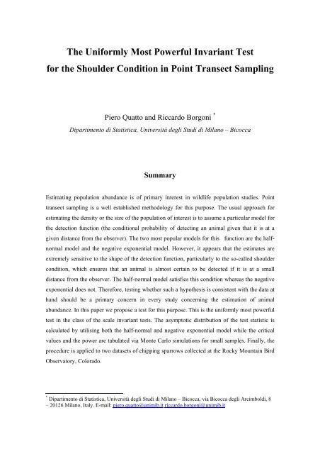
The Uniformly Most Powerful Invariant Testfor the Shoulder Condition in Point Transect SamplingPiero Quatto and Riccardo Borgoni *Dipartimento di Statistica, Università degli Studi di Milano – BicoccaSummaryEstimating population abundance is of primary interest in wildlife population studies. Pointtransect sampling is a well established methodology for this purpose. The usual approach forestimating the density or the size of the population of interest is to assume a particular model forthe detection function (the conditional probability of detecting an animal given that it is at agiven distance from the observer). The two most popular models for this function are the halfnormalmodel and the negative exponential model. However, it appears that the estimates areextremely sensitive to the shape of the detection function, particularly to the so-called shouldercondition, which ensures that an animal is almost certain to be detected if it is at a smalldistance from the observer. The half-normal model satisfies this condition whereas the negativeexponential does not. Therefore, testing whether such a hypothesis is consistent with the data athand should be a primary concern in every study concerning the estimation of animalabundance. In this paper we propose a test for this purpose. This is the uniformly most powerfultest in the class of the scale invariant tests. The asymptotic distribution of the test statistic iscalculated by utilising both the half-normal and negative exponential model while the criticalvalues and the power are tabulated via Monte Carlo simulations for small samples. Finally, theprocedure is applied to two datasets of chipping sparrows collected at the Rocky Mountain BirdObservatory, Colorado.* Dipartimento di Statistica, Università degli Studi di Milano – Bicocca, via Bicocca degli Arcimboldi, 8– 20126 Milano, Italy. E-mail: piero.quatto@unimib.it riccardo.borgoni@unimib.it

Keywords: Point Transect Sampling, Shoulder Condition, Uniformly Most Powerful InvariantTest, Asymptotic Critical Values, Monte Carlo Critical Values.Acknowledgment: The authors thank David Hanni and the Rocky Mountain Bird Observatoryfor having kindly provided the data used in the paper. The authors also thank Kendall Katze forediting the paper.1. INTRODUCTIONNumerous studies of wildlife populations require estimates of population abundance.Transect sampling methodology provides an effective approach for estimatingpopulation size ν or density δ = ν / A, where A is the area of the study region. Athorough review of this approach is given for instance by Barabesi (2000).The point transect design (Buckland, 1987) in particular assumes that k points arerandomly chosen within the study area and, then at each of the selected points, anobserver measures the distance from himself to any animal detected. Since the numberof animals observed from each point is quite small in many contexts where this samplescheme is adopted (as for instance in ornithology), sampled distances are pooledtogether to increase the sample size.Let z 1 ,…,z n be the sample of size n obtained by pooling together the distancesmeasured at each of the k observation points. Let f be the probability density function(pdf) of the observed distances and let g be the detection function, that is to say g(y) isthe conditional probability of detecting an animal given that it is at distance y from theobserver. The relation:f ( z)=zg(z)(1)yg(y)dy∫ + ∞0holds for every distance z. The estimator of the population density δ is:

ˆ δ =nf ˆ ′(0)2kπwhere ˆf ′(0)is an estimator of the derivative of f at 0 which satisfies the fundamentalidentity:f ′(0)=∫ + ∞01yg(y)dy(Buckland et al., 2001, pp. 54-57). The basic problem for estimating δ, or equivalentlyν, is therefore to estimate f’(0).In a previous paper (Borgoni et al., 2005), we investigated the small-samplebehaviour of different δ estimators, depending on the shape of the detection function.We considered the two most popular families of detection functions (Zhang, 2001;Eidous, 2005):the half-normal family:2⎛ y ⎞g ( y)= exp⎜ −⎟ (σ > 0) (2)2⎝ 2σ⎠and the negative exponential family:⎛ y ⎞g( y)= exp⎜− ⎟ (σ > 0). (3)⎝ σ ⎠The former satisfies the shape criterion:g ′( 0) = 0(4)whereas the latter does not. This property, also known as the shoulder condition, ensuresthat animal detection is nearly certain at small distances from the observer (Buckland et

al., 2001, pp. 42, 68-69; Buckland et al., 2004, p. 344). However, such a condition failswhen detectability decreases sharply around the observation points because of low orinexistent visibility (e.g. in presence of fog or dense vegetation).In a point transect framework, Borgoni et al. (2005) demonstrated several simulationresults suggesting that the usual estimators of δ are extremely sensitive to departuresfrom the shape criterion. A similar behaviour was found in the line transect context(Eidous, 2005).Therefore, testing the shape criterion is a preliminary step for any attempt to estimatewildlife population density via transect sampling (Zhang, 2003; Eidous, 2005).The aim of this paper is to propose a procedure for testing the shoulder condition (4).As this condition is independent from the choice of the measure unit for the distance,the scale invariance seems to be a natural restriction for a statistical test. In particular wefocus on a scale invariant test for discriminating between the two families (2) and (3).Because of (1) this turns out to be equivalent to testing that the distance probabilitydensity function (pdf) belongs to one of the two families:2⎧⎛ ⎞ ⎫= ⎨ ( z zF =⎜ −⎟0f z)exp : σ >20 ⎬(5)⎩ σ ⎝ 2σ2⎠ ⎭and:⎧ z ⎛ z ⎞ ⎫F1 = ⎨ f ( z ) = exp ⎜ − ⎟ : σ >20 ⎬. (6)⎩ σ ⎝ σ ⎠ ⎭The proposed test is the uniformly most powerful (UMP) in the class of the scaleinvariant tests. This is discussed in section 2 where the asymptotic distributions of thetest statistic under (5) and (6) are calculated.In section 3 the critical values and the powers of the test are tabulated via MonteCarlo simulations for several typical α-levels and small sample sizes n. In section 4 theproposed procedure is applied to a dataset coming from a large study conducted by theRocky Mountain Bird Observatory, Colorado, in 2002. Conclusions are provided insection 5.

2. THE UMP SCALE INVARIANT TESTGiven n independent observations z 1 ,…,z n from an unknown pdf f, we consider theproblem of testing:H 0 : f ∈ F 0 vs. H 1 : f ∈ F 1 , (7)where F 0 is the family of Rayleigh distributions with scale parameter σ, and F 1 is thefamily of Gamma distributions with shape parameter 2 and scale parameter σ, specifiedin (5) and (6) respectively. This problem is invariant under the group of scaletransformations:{ ( z)= rz : > 0}G = γ r .A maximal invariant under G (Lehmann and Romano, 2005, pp. 214-215) is:( z z z z z )z1 n 2 n,...,n 1,−. (8)nIt can be proved (see the Appendix) that the UMP test among all of the functions ofthis maximal invariant rejects the null hypothesis for large values of the likelihood ratio:⎡ n ⎤2⎢ zi⎥(2n−1)!∑⎢ i=1λ =⎥ . (9)n−1n ⎢ n22 ( −1)!⎛ ⎞⎥⎢⎜∑z ⎥i⎟⎢⎣⎝ i=1 ⎠ ⎥⎦nGiven that λ is a monotonically increasing function of the statistic:

1n2∑ zin i=1Qn= , (10)n2⎛ 1⎜⎝ n∑i=1⎞zi⎟⎠the critical region of the UMP scale invariant test for the hypotheses (7) can be writtenas:Qn ≥ q n,α, (11)where α denotes the level of significance and q n,α is the corresponding critical value sothat:P( Q q ) αn≥n, α| H0= .Furthermore, the asymptotic normal distribution under H 0 is:n32d( 256 / − 80 / π )( Q − 4 / π ) ⎯⎯→N( 0,1)π , (12)nand under H 1 :d( Q 3/ 2) ⎯⎯→( 0,1)4n3 − N ,nwhich are derived from the bivariate central limit theorem and the delta method. Forlarge n the approximate critical value and the power are given respectively by:q n, α≅ 1 .27 + 0. 39 z1−αnand:( Q ≥ q | H ) ≅ 1− Φ( 0.22z0. n )1−β = Pn n, α 11−α− 26 ,

wherez1−αis the (1−α)th quantile and Φ is the cumulative distribution function of thestandard normal distribution. Hence, the proposed test results as being consistent(Lehmann, 2001, p. 158).3. TABLES OF CRITICAL VALUES AND POWERSAs the distribution of the test statistic under (5) or (6) does not depend on the scaleparameter, Monte Carlo simulations can be performed in order to obtain the empiricalcritical values and powers for small sample sizes.The simulation design consists of randomly drawing n distances from the distribution(5) assuming, without loss of generality, σ = 1. The statistic (10) is then applied to eachof the simulated samples and the procedure is repeated 5000 times. The critical valueq n,α for a considered significance level α is obtained as 100×(1-α )-th percentile of theMonte Carlo replicates. We obtained the power of the test in a similar manner. In thiscase, each sample is simulated according to the alternative distribution (6). Monte Carloapproximations of the critical values q n,α and powers are reported in Table 1 and inTable 2. It can be noted that the power under (6) is reasonably good even in the case ofa moderate sample and low α.Table 1. Critical values q n,α of the UMP scale invariant test.q n,α n = 30 n = 40 n = 50 n = 60 n=100α = 0.01 1.46 1.43 1.41 1.40 1.37α = 0.05 1.39 1.37 1.37 1.36 1.34α = 0.10 1.36 1.35 1.34 1.33 1.32

Table 2. Power 1−β of the UMP scale invariant test1−β n = 30 n = 40 n = 50 n = 60 n=100α = 0.01 0.47 0.61 0.71 0.78 0.96α = 0.05 0.68 0.80 0.87 0.91 0.99α = 0.10 0.79 0.87 0.92 0.95 0.99The test also performs well in terms of the power in the case of the data originatingfrom a mixture of (5) and (6). In particular the case where the sample is drawn from apdf was considered:2( − z 2) + ( 1−π ) z exp( − z)π z exp,π being the average proportion of the observed distances simulated from a populationdistributed according to the alternative hypothesis. Table 3 shows the power of the testof level α = 0.05 for a range of mixture proportions π and some sample sizes.Table 3. Power 1−β of the UMP scale invariant test for different mixture proportionsα = 0.05 n = 40 n = 50 n=100π = 0.25 0.80 0.87 0.99π = 0.50 0.75 0.81 0.97π = 0.75 0.54 0.60 0.83It can be observed that the proposed procedure performs well even in the case of asample of moderate size drawn from mixture model with a large π.

4. A CASE STUDYIn this section, we apply the test procedure previously described to two datasets drawnfrom a large study conducted in 2002 by the Rocky Mountain Bird Observatory,Colorado (Panjabi, 2003, p. 100).The first dataset is a point transect sample of 72 chipping sparrows (scientific name:Spizella Passerina) observed during the early morning of 28 May 2002. The 51observation points were allocated in Pine Juniper shrub land in South Dakota. Thedistances collected range from between 8m to 183m (the first and third quartile were20.75m and 75.25m, respectively) with an average distance of 53.18m and standarddeviation equal to 37.59m.The distribution of the observed distances is shown in Figure 1. The box plotsuggests that one potential outlier is present in the data set at hand. This observation istherefore omitted in the subsequent analysis.The test statistic for a null hypothesis of an half-normal detection function equals1.45. The null distribution of this statistic is tabulated according to the method describedin the previous section for a sample size n = 71 and 10000 simulations obtaining acritical value at the 5% significance level equal to 1.35. The null hypothesis shouldtherefore be rejected at the considered level. At this significance level, the power isabout 95%. In fact, in this case, there seems to be a strong evidence of a detectionfunction which is not half-normal as the Monte Carlo p-value is extremely small(0.0007).

(a)(b)Frequency0 5 10 15 20 2550 100 1500 50 100 150 200 250 300Observed distanceFigure 1. Distribution of the observed distances for the chipping sparrow data in PineJuniper shrub landsThe second dataset is a point transect sample of 82 chipping sparrows selected duringthe early morning of 26 May 2002 in a different environment. The 94 observation pointswere allocated in a burn area in South Dakota.The distances collected ranged from between 10m to 200m (the first and thirdquartile were 42m and 100.2m, respectively) with an average distance of 77.2m andstandard deviation equal to 44.84m.The distribution of the observed distances is reported in Figure 2. The box plotsuggests that two potential outliers are present in the data set at hand. Theseobservations were therefore omitted in the subsequent analysis. The third largestobservation in the original sample was nearly at the extreme of upper whisker of the boxplot (183m). This value was identified as a further outlier by a second box plotconstructed on the sample obtained by dropping the two largest observations from theoriginal dataset. This value was also dropped from the subsequent analysis.The test statistic for a null hypothesis of an half-normal detection function equals1.291. In this case as well, the null distribution of this statistic is tabulated according tothe method described in the previous section for a sample size n = 79 and 10000simulations obtaining a 5% critical value equal to 1.345. Hence the null hypothesisshould not be rejected at this considered significance level. The power of the test was

96.2%. at this significance level. In this case, the Monte Carlo p-value results as being0.304 indicating that the data strongly support the null hypothesis.(a)(b)Frequency0 5 10 15 20 2550 100 150 2000 50 100 150 200 250 300Observed distanceFigure 2. Distribution of the observed distances for the chipping sparrow data in burnareasFinally, we can observe that, although the sample size of the two samples are notsmall, the Monte Carlo p-values still differ significantly from the asymptoticapproximation given in (12) by:⎛ q −1.273⎞ˆα = 1− Φ⎜n ⎟ ,⎝ 0.388 ⎠where Φ is the cumulative distribution function of the standard normal distribution andq is the observed value of the test statistic in (10). The p-values are equal to 0.0001 and0.3437 for the first and second sample respectively.

5. CONCLUSIONSIn transect sampling the problem of testing the shoulder condition of a detectionfunction is invariant under the group of scale transformations. Therefore, the scaleinvariance furnishes a natural restriction on the statistical procedure to be utilised.Given that the half-normal and the negative exponential family are the two mostcommonly used models of detection functions, the above problem is reduced to testingbetween the Rayleigh family and a subclass of the Gamma family. For this we proposedthe UMP scale invariant test for which the limiting normal distribution of the teststatistic is provided. The consistency of the test is indicated at the end of section 2. Inthe case of small samples we suggest a Monte Carlo approach for tabulating the criticalvalues and related powers for a range of different sample sizes and significant levels. Itturned out that the critical values and the power approximated via the Monte Carlo andthe asymptotic distribution provide a very similar result for a sample size of 100 ormore. For example, in the case of a sample size equal 100 the empirical and asymptoticcritical values both were 1.34 at the 5% level; examining the power, only a slightdifference was registered between the two approaches (0.99 and 0.97 respectively).Finally, the test was applied to a point transect survey. As expected, the shouldercondition seems largely supported by data collected in an open space with goodvisibility whereas it is rejected in the case of data gathered in dense vegetation.APPENDIXThe pdf of the sample ( z ,..., )1z ncan be written as:L1σ( z1,...,zn) =n ∏ni=1⎛ zi⎞f ⎜ ⎟ ,⎝ σ ⎠where:

2( − z 2)⎧zexp : under H0f ( z)= ⎨.⎩ z exp( − z): under H1Therefore the maximal invariant (8) is expressed as:( r ) ( z z , z z z z )r1 ,...,n− 1=1 n 2 n,...,n−1nand has pdf given by:+∞∫0zn−1nLn n−1( z r ,..., z r , z ) dz = z u f ( z u)n 1n n−1nn+∞∫∏dun⎧⎪ ∏ zin−1i=1⎪2( n −1)!⎪n⎛ 2 ⎞⎪ ⎜∑zi⎟=⎝ i=1 ⎠⎨n⎪∏ zi⎪i=1⎪ (2n−1)!n2n⎪ ⎛ ⎞⎜ ⎟⎪ ∑ zi⎩ ⎝ i=1 ⎠nn0 i=1in: under H: under H10from which the likelihood ratio (9) follows.By the Neyman-Pearson Lemma the most powerful test rejects the null hypothesiswhen (9) is too large. Given that its critical region does not depend on σ, the test isUMP among all invariant tests, as asserted.REFERENCESBarabesi L. 2000. Local likelihood density estimation in line transect sampling.Environmetrics. 11: 413-422.Borgoni R, Cameletti M, Quatto P. 2005. Comparing estimators of animal abundance: asimulation study. Atti del Convegno della Società Italiana di Statistica “Statistica eAmbiente”, Università degli Studi di Messina; 181-184.

Buckland ST. 1987. On the variable circular plot method of estimating animal density.Biometrics. 43, 2: 363-384.Buckland ST, Anderson DR, Burnham KP, Laake JL, Borchers DL, Thomas L. 2001.Introduction to Distance Sampling. Oxford University Press: Oxford.Buckland ST, Anderson DR, Burnham KP, Laake JL, Borchers DL, Thomas L. 2004.Advanced Distance Sampling. Oxford University Press: Oxford.Eidous OM. 2005. On Improving Kernel Estimators Using Line Transect Sampling.Communications in Statistics – Theory and Methods, 34: 931-941.Lehmann EL. 2001. Elements of Large-Sample Theory. Springer: New York.Lehmann EL, Romano JP. 2005. Testing Statistical Hypotheses. Springer: New York.Panjabi, A. 2003. Monitoring the birds of the Black Observatory. Fort Collins,Colorado.Zhang S. 2001. Generalized likelihood ratio test for the shoulder condition in linetransect sampling. Communications in Statistics – Theory and Methods, 30: 2343-2354.Zhang S. 2003. A Note on Testing the Shoulder Condition in Line Transect Sampling.Proceedings of the 2003 Hawaii International Conference on Statistics and relatedtopics.