Modeling Tools for Environmental Engineers and Scientists

© 2002 by CRC Press LLCModeling ToolsforEnvironmentalEngineersandScientists

Library of Congress Cataloging-in-Publication DataNirmala Khandan, N.Modeling tools for environmental engineers and scientists / N. Nirmala Khandan.p. cm.Includes bibliographical references and index.ISBN 1-56676-995-71. Environmental sciences—Mathematical models. 2. Environmentalengineering—Mathematical models. I. Title.GE45.M37 K43 2001628¢.01¢1—dc21 2001052467This book contains information obtained from authentic and highly regarded sources. Reprinted materialis quoted with permission, and sources are indicated. A wide variety of references are listed. Reasonableefforts have been made to publish reliable data and information, but the author and the publisher cannotassume responsibility for the validity of all materials or for the consequences of their use.Neither this book nor any part may be reproduced or transmitted in any form or by any means, electronicor mechanical, including photocopying, microfilming, and recording, or by any information storage orretrieval system, without prior permission in writing from the publisher.The consent of CRC Press LLC does not extend to copying for general distribution, for promotion, forcreating new works, or for resale. Specific permission must be obtained in writing from CRC Press LLCfor such copying.Direct all inquiries to CRC Press LLC, 2000 N.W. Corporate Blvd., Boca Raton, Florida 33431.Trademark Notice: Product or corporate names may be trademarks or registered trademarks, and areused only for identification and explanation, without intent to infringe.Visit the CRC Press Web site at www.crcpress.com© 2002 by CRC Press LLCNo claim to original U.S. Government worksInternational Standard Book Number 1-56676-995-7Library of Congress Card Number 2001052467Printed in the United States of America 1 2 3 4 5 6 7 8 9 0Printed on acid-free paper

ContentsPrefaceAcknowledgmentsFUNDAMENTALS1. INTRODUCTION TO MODELING1.1 What is Modeling?1.2 Mathematical Modeling1.3 Environmental Modeling1.4 Objectives of This BookAppendix 1.1Appendix 1.22. FUNDAMENTALS OF MATHEMATICAL MODELING2.1 Definitions and Terminology in Mathematical Modeling2.2 Steps in Developing Mathematical Models2.3 Application of the Steps in Mathematical Modeling3. PRIMER ON MATHEMATICS3.1 Mathematical Formulations3.2 Mathematical Analysis3.3 Examples of Analytical and Computational Methods3.4 Closure© 2002 by CRC Press LLC

4. FUNDAMENTALS OF ENVIRONMENTAL PROCESSES4.1 Introduction4.2 Material Content4.3 Phase Equilibrium4.4 Environmental Transport Processes4.5 Interphase Mass Transport4.6 Environmental Nonreactive Processes4.7 Environmental Reactive Processes4.8 Material BalanceAppendix 4.15. FUNDAMENTALS OF ENGINEERED ENVIRONMENTALSYSTEMS5.1 Introduction5.2 Classifications of Reactors5.3 Modeling of Homogeneous Reactors5.4 Modeling of Heterogeneous Reactors6. FUNDAMENTALS OF NATURAL ENVIRONMENTALSYSTEMS6.1 Introduction6.2 Fundamentals of Modeling Soil Systems6.3 Fundamentals of Modeling Aquatic SystemsAppendix 6.17. SOFTWARE FOR DEVELOPING MATHEMATICALMODELS7.1 Introduction7.2 Spreadsheet-Based Software7.3 Equation Solver-Based Software7.4 Dynamic Simulation-Based Software7.5 Common Example Problem: Water Quality Modelingin Lakes7.6 ClosureAppendix 7.1Appendix 7.2© 2002 by CRC Press LLC

APPLICATIONS8. MODELING OF ENGINEERED ENVIRONMENTALSYSTEMS8.1 Introduction8.2 Modeling Example: Transients in Sequencing BatchReactors8.3 Modeling Example: CMFRs in Series for ToxicityManagement8.4 Modeling Example: Municipal Wastewater Treatment8.5 Modeling Example: Chemical Oxidation8.6 Modeling Example: Analysis of Catalytic Bed Reactor8.7 Modeling Example: Waste Management8.8 Modeling Example: Activated Carbon Treatment8.9 Modeling Example: Bioregeneration of Activated Carbon8.10 Modeling Example: Pipe Flow Analysis8.11 Modeling Example: Oxygen/Nitrogen Transfer in PackedColumns8.12 Modeling Example: Groundwater Flow Management8.13 Modeling Example: Diffusion through Porous Media9. MODELING OF NATURAL ENVIRONMENTAL SYSTEMS9.1 Introduction9.2 Modeling Example: Lakes in Series9.3 Modeling Example: Radionuclides in Lake Sediments9.4 Modeling Example: Algal Growth in Lakes9.5 Modeling Example: Contaminant Transport Visualization9.6 Modeling Example: Methane Emissions from Rice Fields9.7 Modeling Example: Chemical Equilibrium9.8 Modeling Example: Toxicological Exposure Evaluation9.9 Modeling Example: Visualization of Groundwater Flow9.10 Modeling Example: Air Pollution—Puff Model9.11 Modeling Example: Air Pollution—Plume Model9.12 Modeling Example: Fugacity-Based Modeling9.13 Modeling Example: Well Placement and Water QualityManagementBIBLIOGRAPHY© 2002 by CRC Press LLC

PrefaceTHIS book is not a treatise on environmental modeling. Several excellentbooks are currently available that do more than justice to the science ofenvironmental modeling. The goal of this book is to bridge the gap betweenthe science of environmental modeling and working models of environmentalsystems. More specifically, the intent of this book is to bring computerbasedmodeling within easy reach of subject matter experts and professionalswho have shied away from modeling, daunted by the intricacies of computerprogramming and programming languages.In the past two decades, interest in computer modeling in general and inenvironmental modeling in particular, have grown significantly. The numberof papers and reports published on modeling, the number of specialty conferenceson modeling held all over the world, and the number of journalsdedicated to modeling efforts are evidence of this growth. Several factorssuch as better understanding of the underlying science, availability of highperformance computer facilities, and increased regulatory concerns andpressures have fueled this growth. Scrutiny of those involved in environmentalmodeling, however, reveals that only a small percentage of expertsare active in the modeling efforts; namely those who also happen to beskilled in computer programming.For the rest of us, computer modeling has remained a challenging taskuntil recently. A new breed of software authoring packages has now becomeavailable that enables nonprogrammers to develop their own models withouthaving to learn programming languages. These packages feature English-likesyntax and easy-to-use yet extremely powerful mathematical, analytical,computational, and graphical functions, and user-friendly interfaces. Theycan drastically reduce the time, effort, and programming skills required todevelop professional quality user-friendly models. This book describes eightsuch software packages, and, with over 50 modeling examples, illustrateshow they can be adapted for almost any type of modeling project.© 2002 by CRC Press LLC

The contents of this book are organized into nine chapters. Chapter 1 is anintroduction to modeling. Chapter 2 focuses on the science and art of mathematicalmodeling. Chapter 3 contains a primer on mathematics with examplesof computer implementation of standard mathematical calculi. Chapters 4, 5,and 6 contain reviews of the fundamentals of environmental processes, engineeredsystems, and natural systems, respectively. Chapter 7 describes andcompares the eight software packages selected here for developing environmentalmodels. Chapters 8 and 9 are devoted entirely to modeling examplescovering engineered and natural systems, respectively.The book can be of benefit to those who have been yearning to venture intomodeling, as well as to those who have been using traditional language-basedapproaches for modeling. In the academic world, this book can be used as themain text to cultivate computer modeling skills at the freshman or junior levels.It can be used as a companion text in “fate and transport” or “environmentalmodeling” types of courses. It can be useful to graduate studentsplanning to incorporate some form of modeling into their research. Facultycan benefit from this book in developing special purpose models for teaching,research, publication, or consulting. Practicing professionals may find it usefulto develop custom models for limited use, preliminary analysis, and feasibilitystudies. Suggested uses of this book by different audiences at differentlevels are included in Chapter 1.As a final note, this book should not be taken as a substitute for the usermanuals that accompany software packages; rather, it takes off from wherethe user manuals stop, and demonstrates the types of finished products (models,in this case) that can be developed by integrating the features of the software.This book can, perhaps, be compared to a road map, which can takenonprogrammers from the problem statement to a working computer-basedmathematical model. Different types of vehicles can be used for the journey.The intention here is not to teach how to drive the vehicles but rather to pointout the effort required by the different vehicles, their capabilities, advantages,disadvantages, special features, and limitations.© 2002 by CRC Press LLC

AcknowledgmentsIwould like to acknowledge several individuals who, directly or indirectly,were responsible for giving me the strength, confidence, opportunity, and supportto venture into this project. First, I would like to recognize all my teachersin Sri Lanka, some of whom probably did not even know me by name. Yet, theygave me a rigorous education, particularly in mathematics, for which I amforever thankful. I also want to acknowledge the continuing encouragement,guidance, motivation, and friendship of Professor Richard Speece, to whomI gratefully attribute my academic career. The five years that I shared withProfessor Speece have been immensely satisfying and most productive. I wantto thank my department head, Professor Kenneth White, for supporting myefforts throughout my academic tenure, without which I could not have foundthe time or the resources to embark on this project. Thanks to my departmentalcolleagues and the administration at New Mexico State University for allowingme to go on sabbatical leave to complete this project.The donation of full versions of software packages by MathSoft, Inc., TheMathworks, Inc., Universal Technical Systems, Inc., Wolfram Research, Inc.,and High Performance Systems, Inc., is gratefully acknowledged. The support,encouragement, and patience of Dr. Joseph Eckenrode and his editorialstaff at Technomic Publishing Co., Inc. (now owned by CRC Press LLC) isfully appreciated.I am indebted to my grandparents and to my parents for the sacrifices theymade to ensure that I received the finest education from the earliest age; andto the families of my sister and sister-in-law for their support and compassion,particularly during my graduate studies. Finally, I am thankful to my wifeGnana and our sons Rajeev and Sanjeev, for their support, understanding, andtolerance throughout this and many other projects, which took much of mytime and attention away from them. Sanjeev also contributed to this workdirectly in setting up some of the models and by sharing some of the agoniesand ecstasies of computer programming.© 2002 by CRC Press LLC

PART IFundamentals© 2002 by CRC Press LLC

CHAPTER 1Introduction to ModelingCHAPTER PREVIEWIn this chapter, an overview of the process of modeling is presented.Different approaches to modeling are identified first, and features ofmathematical modeling are detailed. Alternate classifications of mathematicalmodels are addressed. A case history is presented to illustratethe benefits and scope of environmental modeling. A road map throughthis book is presented, identifying the topics to be covered in the followingchapters and potential uses of the book.1.1 WHAT IS MODELING?MODELING can be defined as the process of application of fundamentalknowledge or experience to simulate or describe the performance of areal system to achieve certain goals. Models can be cost-effective and efficienttools whenever it is more feasible to work with a substitute than with thereal, often complex systems. Modeling has long been an integral componentin organizing, synthesizing, and rationalizing observations of and measurementsfrom real systems and in understanding their causes and effects.In a broad sense, the goals and objectives of modeling can be twofold:research-oriented or management-oriented. Specific goals of modeling effortscan be one or more of the following: to interpret the system; to analyze itsbehavior; to manage, operate, or control it to achieve desired outcomes; todesign methods to improve or modify it; to test hypotheses about the system;or to forecast its response under varying conditions. Practitioners, educators,researchers, and regulators from all professions ranging from business tomanagement to engineering to science use models of some form or another intheir respective professions. It is probably the most common denominatoramong all endeavors in such professions, especially in science and engineering.© 2002 by CRC Press LLC

The models resulting from the modeling efforts can be viewed as logicaland rational representations of the system. A model, being a representationand a working hypothesis of a more complex system, contains adequate butless information than the system it represents; it should reflect the featuresand characteristics of the system that have significance and relevance to thegoal. Some examples of system representations are verbal (e.g., languagebaseddescription of size, color, etc.), figurative (e.g., electrical circuit networks),schematic (e.g., process and plant layouts), pictographic (e.g.,three-dimensional graphs), physical (e.g., scaled models), empirical (e.g., statisticalmodels), or symbolic (e.g., mathematical models). For instance, instudying the ride characteristics of a car, the system can be representedverbally with words such as “soft” or “smooth,” figuratively with spring systems,pictographically with graphs or videos, physically with a scaled materialmodel, empirically with indicator measurements, or symbolically usingkinematic principles.Most common modeling approaches in the environmental area can be classifiedinto three basic types—physical modeling, empirical modeling, andmathematical modeling. The third type forms the foundation for computermodeling, which is the focus of this book. While the three types of modelingare quite different from one another, they complement each other well. Aswill be seen, both physical and empirical modeling approaches providevaluable information to the mathematical modeling process. These threeapproaches are reviewed in the next section.1.1.1 PHYSICAL MODELINGPhysical modeling involves representing the real system by a geometricallyand dynamically similar, scaled model and conducting experiments onit to make observations and measurements. The results from these experimentsare then extrapolated to the real systems. Dimensional analysis andsimilitude theories are used in the process to ensure that model results can beextrapolated to the real system with confidence.Historically, physical modeling had been the primary approach followedby scientists in developing the fundamental theories of natural sciences.These included laboratory experimentation, bench-scale studies, and pilotscaletests. While this approach allowed studies to be conducted under controlledconditions, its application to complex systems has been limited. Someof these limitations include the need for dimensional scale-up of “small” systems(e.g., colloidal particles) or scale-down of “large” ones (e.g., acid rain),limited accessibility (e.g., data collection); inability to accelerate or slowdown processes and reactions (e.g., growth rates), safety (e.g., nuclear reactions),economics (e.g., Great Lakes reclamation), and flexibility (e.g.,change of diameter of a pilot column).© 2002 by CRC Press LLC

1.1.2 EMPIRICAL MODELINGEmpirical modeling (or black box modeling) is based on an inductive ordata-based approach, in which past observed data are used to develop relationshipsbetween variables believed to be significant in the system beingstudied. Statistical tools are often used in this process to ensure validity of thepredictions for the real system. The resulting model is considered a “blackbox,” reflecting only what changes could be expected in the system performancedue to changes in inputs. Even though the utility value of this approachis limited to predictions, it has proven useful in the case of complex systemswhere the underlying science is not well understood.1.1.3 MATHEMATICAL MODELINGMathematical modeling (or mechanistic modeling) is based on the deductiveor theoretical approach. Here, fundamental theories and principles governingthe system along with simplifying assumptions are used to derivemathematical relationships between the variables known to be significant.The resulting model can be calibrated using historical data from the real systemand can be validated using additional data. Predictions can then be madewith predefined confidence. In contrast to the empirical models, mathematicalmodels reflect how changes in system performance are related to changesin inputs.The emergence of mathematical techniques to model real systems have alleviatedmany of the limitations of physical and empirical modeling.Mathematical modeling, in essence, involves the transformation of the systemunder study from its natural environment to a mathematical environment interms of abstract symbols and equations. The symbols have well-definedmeanings and can be manipulated following a rigid set of rules or “mathematicalcalculi.” Theoretical concepts and process fundamentals are used toderive the equations that establish relationships between the system variables.By feeding known system variables as inputs, these equations or “models”can then be solved to determine a desired, unknown result. In the precomputerera, mathematical modeling could be applied to model only those problemswith closed-form solutions; application to complex and dynamicsystems was not feasible due to lack of computational tools.With the growth of high-speed computer hardware and programming languagesin the past three decades, mathematical techniques have been appliedsuccessfully to model complex and dynamic systems in a computer environment.Computers can handle large volumes of data and manipulate them at aminute fraction of the time required by manual means and present the resultsin a variety of different forms responsive to the human mind. Development ofcomputer-based mathematical models, however, remained a demanding task© 2002 by CRC Press LLC

within the grasp of only a few with subject-matter expertise and computerprogramming skills.During the last decade, a new breed of software packages has becomeavailable that enables subject matter experts with minimal programmingskills to build their own computer-based mathematical models. These softwarepackages can be thought of as tool kits for developing applications andare sometimes called software authoring tools. Their functionality is somewhatsimilar to the following: a web page can be created using hypertextmarking language (HTML) directly. Alternatively, one can use traditionalword-processing programs (such as Word ®1 ), or special-purpose authoringprograms (such as PageMill ®2 ), and click a button to create the web pagewithout requiring any knowledge of HTML code.Currently, several different types of such syntax-free software authoringtools are commercially available for mathematical model building. They arerich with built-in features such as a library of preprogrammed mathematicalfunctions and procedures, user-friendly interfaces for data entry and running,post-processing of results such as plotting and animation, and high degrees ofinteractivity. These authoring tools bring computer-based mathematical modelingwithin easy reach of more subject matter experts and practicing professionals,many of whom in the past shied away from it due to lack of computerprogramming and/or mathematical skills.1.2 MATHEMATICAL MODELINGThe elegance of mathematical modeling needs to be appreciated: a singlemathematical formulation can be adapted for a wide number of real systems,with the symbols taking on different meanings depending on the system. Asan elementary example, consider the following linear equation:Y mX C (1.1)The “mathematics” of this equation is very well understood as is its “solution.”The readers are probably aware of several real systems where Equation(1.1) can serve as a model (e.g., velocity of a particle falling under gravitationalacceleration or logarithmic growth of a microbial population). Asanother example, the partial differential equation2 ∂ φ = α ∂ φ∂t∂x2 (1.2)1 Word ® is a registered trademark of Microsoft Corporation. All rights reserved.2 PageMill ® is a registered trademark of Adobe Systems Incorporated. All rights reserved.© 2002 by CRC Press LLC

can model the temperature profile in a one-dimensional heat transfer problemor the concentration of a pollutant in a one-dimensional diffusion problem.Thus, subject matter experts can reduce their models to standard mathematicalforms and adapt the standard mathematical calculi for their solution,analysis, and evaluation.Mathematical models can be classified into various types depending on thenature of the variables, the mathematical approaches used, and the behaviorof the system. The following section identifies some of the more common andimportant types in environmental modeling.1.2.1 DETERMINISTIC VS. PROBABILISTICWhen the variables (in a static system) or their changes (in a dynamic system)are well defined with certainty, the relationships between the variablesare fixed, and the outcomes are unique, then the model of that system is saidto be deterministic. If some unpredictable randomness or probabilities areassociated with at least one of the variables or the outcomes, the model is consideredprobabilistic. Deterministic models are built of algebraic and differentialequations, while probabilistic models include statistical features.For example, consider the discharge of a pollutant into a lake. If all of thevariables in this system, such as the inflow rate, the volume of the lake, etc.,are assumed to be average fixed values, then the model can be classified asdeterministic. On the other hand, if the flow is taken as a mean value withsome probability of variation around the mean, due to runoff, for example, aprobabilistic modeling approach has to be adapted to evaluate the impact ofthis variable.1.2.2 CONTINUOUS VS. DISCRETEWhen the variables in a system are continuous functions of time, then themodel for the system is classified as continuous. If the changes in the variablesoccur randomly or periodically, then the corresponding model is termeddiscrete. In continuous systems, changes occur continuously as time advancesevenly. In discrete models, changes occur only when the discrete eventsoccur, irrespective of the passage of time (time between those events is seldomuniform). Continuous models are often built of differential equations;discrete models, of difference equations.Referring to the above example of a lake, the volume or the concentrationin the lake might change with time, but as long as the inflow remains nonzero,the system will be amenable to continuous modeling. If random eventssuch as rainfall are to be included, a discrete modeling approach may have tobe followed.© 2002 by CRC Press LLC

1.2.3 STATIC VS. DYNAMICWhen a system is at steady state, its inputs and outputs do not vary withpassage of time and are average values. The model describing the systemunder those conditions is known as static or steady state. The results of astatic model are obtained by a single computation of all of the equations.When the system behavior is time-dependent, its model is called dynamic.The output of a dynamic model at any time will be dependent on the outputat a previous time step and the inputs during the current time step. The resultsof a dynamic model are obtained by repetitive computation of all equationsas time changes. Static models, in general, are built of algebraic equationsresulting in a numerical form of output, while dynamic models are built ofdifferential equations that yield solutions in the form of functions.In the example of the lake, if the inflow and outflow remain constant, theresulting concentration of the pollutant in the lake will remain at a constantvalue, and the system can be modeled by a static model. But, if the inflow ofthe pollutant is changed from its steady state value to another, its concentrationin the lake will change as a function of time and approach another steadystate value. A dynamic model has to be developed if it is desired to trace theconcentration profile during the change, as a function of time.1.2.4 DISTRIBUTED VS. LUMPEDWhen the variations of the variables in a system are continuous functionsof time and space, then the system has to be modeled by a distributed model.For instance, the variation of a property, C, in the three orthogonal directions(x, y, z), can be described by a distributed function C = f(x,y,z). If those variationsare negligible in those directions within the system boundary, thenC is uniform in all directions and is independent of x, y, and z. Such a systemis referred to as a lumped system. Lumped, static models are often built ofalgebraic equations; lumped, dynamic models are often built of ordinary differentialequations; and distributed models are often built of partial differentialequations.In the case of the lake example, if mixing effects are (observed or thoughtto be) significant, then a distributed model could better describe the system.If, on the other hand, the lake can be considered completely mixed, a lumpedmodel would be adequate to describe the system.1.2.5 LINEAR VS. NONLINEARWhen an equation contains only one variable in each term and each variableappears only to the first power, that equation is termed linear, if not, it isknown as nonlinear. If a model is built of linear equations, the model© 2002 by CRC Press LLC

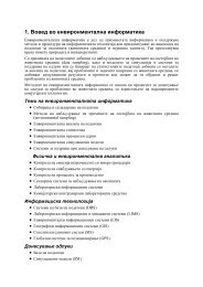
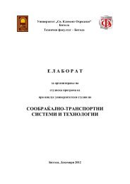
esponses are additive in their effects, i.e., the output is directly proportionalto the input, and outputs satisfy the principle of superpositioning. Forinstance, if an input I 1 to a system produces an output O 1 , and another inputI 2 produces an output of O 2 , then a combined input of (αI 1 + βI 2 ) will producean output of (αO 1 + βO 2 ). Superpositioning cannot be applied in nonlinearmodels.In the lake example, if the reactions undergone by the pollutant in the lakeare assumed to be of first order, for instance, then the linearity of the resultingmodel allows superpositioning to be applied. Suppose the input to the lakeis changed from a steady state condition, then the response of the lake can befound by adding the response following the general solution (due to the initialconditions) to the response following the particular solution (due tothe input change) of the differential equation governing the system.1.2.6 ANALYTICAL VS. NUMERICALWhen all the equations in a model can be solved algebraically to yield asolution in a closed form, the model can be classified as analytical. If that isnot possible, and a numerical procedure is required to solve one or more ofthe model equations, the model is classified as numerical.In the above example of the lake, if the entire volume of the lake isassumed to be completely mixed, a simple analytical model may be developedto model its steady state condition. However, if such an assumptionis unacceptable, and if the lake has to be compartmentalized into severallayers and segments for detailed study, a numerical modeling approach hasto be followed.A comparison of the above classifications is summarized in Figure 1.1.Indicated at the bottom section of this figure are the common mathematicalanalytical methods appropriate for each type of model. These classificationsare presented here to stress the necessity of understanding input data requirements,model formulation, and solution procedures, and to guide in the selectionof the appropriate computer software tool in modeling the system. Mostenvironmental systems can be approximated in a satisfactory manner by linearand time variant descriptions in a lumped or distributed manner, at leastfor specified and restricted conditions. Analytical solutions are possible forlimited types of systems, while solutions may be elaborate or not currentlyavailable for many others. Computer-based mathematical modeling usingnumerical solutions can provide valuable insight in such cases.The goal of this book is to illustrate, with examples, the application of avariety of software packages in developing computer-based mathematicalmodels in the environmental field. The examples included in the book fallinto the following categories: static, dynamic, continuous, deterministic(probabilistic, at times), analytical, numerical, and linear.© 2002 by CRC Press LLC

Real SystemsMathematical ModelsDeterministicProbabilisticContinuousDiscreteStaticDynamicStatisticsN = 1 N > 1 Lumped Distributed MarkovAlgebraic System of Ordinary Partial Difference Monte Carloequations algebraic differential differential equationsequations equations equationsLinearNonlinearAnalyticalNumericalFigure 1.1 Classification of mathematical models (N = number of variables).1.3 ENVIRONMENTAL MODELINGThe application of mathematical modeling in various fields of study hasbeen well illustrated by Cellier (1991). According to Cellier’s account, suchmodels range from the well-defined and rigorous “white-box” models to theill-defined, empirical “black-box” models. With white-box models, it is suggestedthat one could proceed directly to design of full-scale systems withconfidence, while with black-box models, that remains a speculative theory.A modified form of the illustration of Cellier is shown in Table 1.1.Mathematical modeling in the environmental field can be traced back tothe 1900s, the pioneering work of Streeter and Phelps on dissolved oxygenbeing the most cited. Today, driven mainly by regulatory forces, environmentalstudies have to be multidisciplinary, dealing with a wide range ofpollutants undergoing complex biotic and abiotic processes in the soil, surfacewater, groundwater, ocean water, and atmospheric compartments of theecosphere. In addition, environmental studies also encompass equally diverseengineered reactors and processes that interact with the natural environment© 2002 by CRC Press LLC

Table 1.1 Range of Mathematical ModelsModels Systems Calculi ApplicationsWhite-boxElectrical}Ordinary Highly Designdifferentialdeductive andMechanical}equations deterministicControlChemical}PartialdifferentialBiologicalEnvironmental}equationsOrdinaryAnalysisEcologicaldifferentialequationsEconomic}PredictionDifferenceSocialequationsHighlyAlgebraicinductive andSpeculationPsychologicalequationsprobabilisticBlack-box© 2002 by CRC Press LLC

through several pathways. Consequently, modeling of large-scale environmentalsystems is often a complex and challenging task. The impetus fordeveloping environmental models can be one or more of the following:(1) To gain a better understanding of and glean insight into environmentalprocesses and their influence on the fate and transport of pollutants in theenvironment(2) To determine short- and long-term chemical concentrations in the variouscompartments of the ecosphere for use in regulatory enforcement andin the assessment of exposures, impacts, and risks of existing as well asproposed chemicals(3) To predict future environmental concentrations of pollutants under variouswaste loadings and/or management alternatives(4) To satisfy regulatory and statutory requirements relating to environmentalemissions, discharges, transfers, and releases of controlled pollutants(5) To use in hypothesis testing relating to processes, pollution control alternatives,etc.(6) To implement in the design, operation, and optimization of reactors,processes, pollution control alternatives, etc.(7) To simulate complex systems at real, compressed, or expanded time horizonsthat may be too dangerous, too expensive, or too elaborate to studyunder real conditions(8) To generate data for post-processing, such as statistical analysis, visualization,and animation, for better understanding, communication, and disseminationof scientific information(9) To use in environmental impact assessment of proposed new activitiesthat are currently nonexistentAbove all, the formal exercise of designing and building a model may bemore valuable than the actual model itself or its use in that the knowledgeabout the problem is organized and crystallized to extract the maximum benefitfrom the effort and the current knowledge about the subject. Typicalissues and concerns in various environmental systems and the use of mathematicalmodels in addressing them are listed in Appendix 1.1, showing thewide scope of environmental modeling.The use of and need for mathematical models, their scope and utility value,and the computer-based approaches used in developing them can best beillustrated by a case history (Nirmalakhandan et al., 1990, 1991a, 1991b,1992a, 1992b, 1993).Case History: Improvement of the Air-Stripping ProcessThe air-stripping (A/S) process has been used in the chemical engineeringfield for over 50 years. During the early 1980s, this process was adapted byenvironmental engineers for remediating groundwaters contaminated with© 2002 by CRC Press LLC

organic contaminants. While A/S is a cost-effective process for removingvolatile organic contaminants (VOCs), its application at sites contaminatedwith semivolatile organic contaminants (SVOCs) had been limited by prohibitiveenergy requirements. This case study summarizes how mathematicalmodeling was utilized in developing and demonstrating a unique modificationto the A/S process that had the potential for gaining significant improvementsin applicability, efficiency, energy consumption, and overall treatment costs.In the A/S process, the VOC-contaminated water is pumped to the top of apacked tower from where it flows down through the packing media undergravity. A countercurrent stream of air blown from the bottom of the towerstrips the VOCs, and the treated water is collected at the bottom of thetower. From the mass transfer theory, it is known that the efficiency of theprocess and its applicability to SVOCs can be improved by increasingthe driving force for mass transfer. The driving force can be improved byincreasing the airflow rate. But, increasing the airflow rate will not onlyincrease pressure drop and energy consumption, but it will also lead toprocess failure due to flooding of the tower.It was hypothesized that if the airflow could be distributed along the depthof the packing, the driving force for mass transfer could be increased: thefresh air entering the tower along its depth will dilute the upcoming contaminatedair through the tower, thus increasing the driving force throughout thefull depth of the tower. At the same time, the overall pressure drop will not bethat high. In combination, these two factors could be expected to reduce thepacking depth requirements, pressure drop, and energy consumption, leadingto reduced capital and operating costs.To verify this hypothesis, a mathematical model based on fundamentalmass theories was formulated. The model was then used to compare the conventionalA/S process against the proposed process configuration under identicalinput conditions. This modeling exercise confirmed that the proposedconfiguration could result in a 50% reduction in packing depth, a 40% reductionin pressure drop, and a 40% reduction in energy requirement, for comparableremoval efficiencies. Based on these model results, the AmericanWater Works Association (AWWA) funded a research project to verify thehypothesis and validate the process model at pilot scale. The model was usedto optimize the process and design the optimal pilot-scale process. This pilotscaletest confirmed the hypothesis and validated the model predictions. Thevalidated model was then used to design a prototype-scale system and a fieldscalesystem that produced results that were used to further validate the mathematicalmodel over a wide range of operating variables under field conditions.1.4 OBJECTIVES OF THIS BOOKThe premise of this book is that computer-based mathematical modeling isa powerful and essential tool appropriate for analyzing and evaluating a wide© 2002 by CRC Press LLC

ange of complex environmental applications. Desktop and laptop computerswith computing capabilities approaching supercomputer-level performance arenow available at reasonable prices. Several new powerful software packageshave emerged that bring mathematical modeling within reach of nonprogrammers.The primary objective of this book is to introduce several types of computersoftware packages that subject matter experts with minimal computerprogramming skills can use to develop their own models. Even though thisbook has the words “environmental modeling” in its title and is illustratedwith examples in that area, professionals in other fields can also learn aboutthe features of the various software packages identified, benefit from theexamples included, and be able to adapt them in their own areas.The motivation for a book of this nature is that the users manuals thataccompany software often are not focused toward application of the softwarein modeling. In modeling, one has to integrate several features to achieve themodeling goal. In all fairness, the manuals are well written to illustrate thefunctioning of individual features of the software. They cannot be expected toinclude examples of integration of features for specific purposes. This booktakes off from where the manuals end and provides examples of integratedapplications of the software to specific problems.Further impetus for this book stems from the fact that computer usage, particularlyin modeling, analyzing, synthesizing, and simulating in engineeringcurricula, is being advocated by cognitive researchers as one of the effectiveways of improving the teaching and learning processes. Recognizing this, theAccreditation Board of Engineering Technologies (ABET) is placing strongemphasis on computer usage in engineering curricula. Several engineeringprograms have recently initiated freshman undergraduate-level courses tointroduce computer applications in engineering. This book includes basicmathematical concepts and scientific principles for use in such classes to cultivatemodeling skills from early stages.Chapter 2 of the book contains a discussion of the various steps involvedin developing mathematical models. As pointed out in Chapter 2, modeling ispart science and part art, and as such, modelers have developed their ownstyle of accomplishing the task. While it is recognized that differentapproaches are being practiced, the steps and tasks identified in Chapter 2 arekey elements in the process and have to be taken into consideration in someform or another. The procedures presented in Chapter 2 are in no wayintended to be followed in every case.Chapters 3, 4, 5, and 6 present reviews of fundamental concepts in mathematics,environmental processes, engineered environmental systems, andnatural environmental systems, respectively. The material included in thisbook is not to be construed as a formal and/or complete treatment of therespective topics but as a review of the fundamentals involved, providing abasic starting point in the modeling process.© 2002 by CRC Press LLC

Chapter 7 contains a comparative presentation of various types of softwareauthoring packages that can be used for developing mathematical models.These include spreadsheets, mathematical software, and dynamic modelingsoftware. A total of six different packages are identified and compared usingone common problem. Rather than attempt to include every software packagecommercially available, selected examples of software products representingthe different types of systems are included.Chapters 8 and 9 contain several examples of applications of the differenttypes of software packages in modeling engineered and natural systems,respectively. Here, the main focus is on the use of the various packages in thecomputer implementation of the modeling process rather than on the fundamentalsof the science behind the systems. However, a brief review of and referencesto related theories and principles are included, along with pertinentdetails on the model formulation process as a prerequisite to the computerimplementation process.Suggested uses of this book by various audiences are indicated inAppendix 1.2. It is hoped that the book will be able to serve as a primary textbookin environmental modeling courses; a companion book in unit operationsor environmental fate and transport courses; a guidebook to facultyinterested in modeling work for teaching, research, and publication; a tool forgraduate students involved in modeling-oriented research; and a referencebook for practicing professionals in the environmental area.© 2002 by CRC Press LLC

APPENDIX 1.1 TYPICAL USES OF MATHEMATICAL MODELSEnvironmentalMedium Issues/Concerns Use of Models inAtmosphere Hazardous air pollutants; Concentration profiles;air emissions; toxicexposure; design andreleases; acid rain; smog; analysis of control processesCFCs; particulates; health and equipment; evaluationconcerns; global warming of management actions;environmental impactassessment of new projects;compliance with regulationsSurface Wastewater treatment Fate and transport ofwater plant discharges; industrial pollutants; concentrationdischarges; agricultural/ plumes; design and analysisurban runoff; storm water of control processes anddischarges; potable water equipment; wasteloadsource; food chainallocations; evaluation ofmanagement actions;environmental impactassessment of new projects;compliance with regulationsGroundwater Leaking underground Fate and transport ofstorage tanks; leachates pollutants; design andfrom landfills andanalysis of remedial actions;agriculture; injection; drawdowns; compliance withpotable water source regulationsSubsurface Land application of solid Fate and transport ofand hazardous wastes; pollutants; concentrationspills; leachates from plumes; design and analysislandfills; contamination of of control processes;potable acquifersevaluation of managementactionsOcean Sludge disposal; spills; Fate and transport ofoutfalls; food chainpollutants; concentrationplumes; design and analysisof control processes;evaluation of managementactions© 2002 by CRC Press LLC

APPENDIX 1.2 SUGGESTED USES OF THE BOOKTarget AudienceSubjectSubject mattermatter Subject expertsUpper- experts matter who havelevel BS with experts used at Practicingand Advanced- minimal using least one engineers,Lower- beginning level MS computer language- authoring projectlevel BS MS and PhD modeling based software managers,Chapter Topics students students students expertise software program regulators2 Fundamentals Read and Read and Read and Read and Reviewof mathematical review review review reviewmodeling3 Primer on Read and Read and Review Reviewmathematics review review4 Fundamentals Read and Read and Review Reviewof environmental review reviewprocesses5 Fundamentals Read and Read and Review Reviewof engineered review reviewsystems6 Fundamentals of Read and Read and Read and Reviewnatural systems review review review© 2002 by CRC Press LLC

APPENDIX 1.2 (continued)Target AudienceSubjectSubject mattermatter Subject expertsUpper- experts matter who havelevel BS with experts used at Practicingand Advanced- minimal using least one engineers,Lower- beginning level MS computer language- authoring projectlevel BS MS and PhD modeling based software managers,Chapter Topics students students students expertise software program regulators7 Software for Read and Read and Read and Read and Read and Read and Read anddeveloping review review review review review review reviewmathematicalmodels8 Modeling of Read and Read and Read and Read and Review Reviewengineered review review review reviewsystems9 Modeling of Read and Read and Read and Read and Review Reviewnatural systems review review review review© 2002 by CRC Press LLC

CHAPTER 2Fundamentals of MathematicalModelingCHAPTER PREVIEWIn this chapter, formal definitions and terminology relating to mathematicalmodeling are presented. The key steps involved in developingmathematical models are identified, and the tasks to be completedunder each step are detailed. While the suggested procedure is not astandard one, it includes the crucial components to be addressed in theprocess. The application of these steps in developing a mathematicalmodel for a typical environmental system is illustrated.2.1 DEFINITIONS AND TERMINOLOGY INMATHEMATICAL MODELINGGENERAL background information on models was presented in Chapter 1,where certain terms were introduced in a general manner. Before continuingon to the topic of developing mathematical models, it is necessary toformalize certain terminology, definitions, and conventions relating to themodeling process. Recognition of these formalities can greatly help in theselection of the modeling approach, data needs, theoretical constructs, mathematicaltools, solution procedures, and, hence, the appropriate computersoftware package(s) to complete the modeling task. In the following sections,the language in mathematical modeling is clarified in the context of modelingof environmental systems.2.1.1 SYSTEM/BOUNDARYA “system” can be thought of as a collection of one or more relatedobjects, where an “object” can be a physical entity with specific attributes or© 2002 by CRC Press LLC

characteristics. The system is isolated from its surroundings by the “boundary,”which can be physical or imaginary. (In many books on modeling, theterm “environment” is used instead of “surroundings” to indicate everythingoutside the boundary; the reason for picking the latter is to avoid the confusionin the context of this book that focuses on modeling the environment. Inother words, environment is the system we are interested in modeling, whichis enclosed by the boundary.) The objects within a system may or may notinteract with each other and may or may not interact with objects in the surroundings,outside the boundary. A system is characterized by the fact that themodeler can define its boundaries, its attributes, and its interactions withthe surroundings to the extent that the resulting model can satisfy the modeler’sgoals.The largest possible system of all, of course, is the universe. One can,depending on the modeling goals, isolate a part of the universe such as a continent,or a country, or a city, or the city’s wastewater treatment plant, or theaeration tank of the city’s wastewater treatment plant, or the microbial populationin the aeration tank, and define that as a system for modeling purposes.Often, the larger the system, the more complex the model. However, the effortcan be made more manageable by dissecting the system into smaller subsystemsand including the interactions between them.2.1.2 OPEN/CLOSED, FLOW/NONFLOW SYSTEMSA system is called a closed system when it does not interact with the surroundings.If it interacts with the surroundings, it is called an open system. Inclosed systems, therefore, neither mass nor energy will cross the boundary;whereas in open systems, mass and energy can. When mass does not cross theboundary (but energy does), an open system may be categorized as a nonflowsystem. If mass crosses the boundary, it is called a flow system.While certain batch processes may be approximated as closed systems,most environmental systems interact with the surroundings in one way oranother, with mass flow across the boundary. Thus, most environmental systemshave to be treated as open, flow systems.2.1.3 VARIABLES/PARAMETERS/INPUTS/OUTPUTSThe attributes of the system and of the surroundings that have significantimpact on the system are termed “variables.” The term variable includes thoseattributes that change in value during the modeling time span and those thatremain constant during that period. Variables of the latter type are oftenreferred to as parameters. Some parameters may relate to the system, andsome may relate to the surroundings.© 2002 by CRC Press LLC

A system may have numerous attributes or variables. However, as mentionedbefore, the modeler needs to select only those that are significant andrelevant to the modeler’s goal in the modeling process. For example, in thecase of the aeration tank, its attributes can include biomass characteristics, volumeof mixed liquor, its color, temperature, viscosity, specific weight, conductivity,reflectivity, etc., and the attributes of the surroundings may be flowrate, mass input, wind velocity, solar radiation, etc. Even though many of theattributes may be interacting, only a few (e.g., biomass characteristics, volume,flow rate, mass input) are identified as variables of significance and relevancebased on the modeler’s goals (e.g., the efficiency of the aeration tank).Variables that change in value fall into two categories: those that are generatedby the surroundings and influence the behavior of the system, andthose that are generated by the system and impact the surroundings. The formerare called “inputs,” and the latter are called “outputs.” In the case of theaeration tank, the mass inflow can be an input, the concentration leavingthe tank, an output, and the volume of the tank, a parameter. In mathematicallanguage, inputs are considered independent variables, and outputs are considereddependent variables. The inputs and model parameters are oftenknown or defined in advance; they drive the model to produce some output.In the context of modeling, relationships are sought between inputs and outputs,with the parameters acting as model coefficients.At this point, a very important factor has to be recognized; in the real system,not all significant and relevant variables and/or parameters may beaccessible for control or manipulation; likewise, not all outputs may be accessiblefor observation or measurement. However, in mathematical models, allinputs and parameters are readily available for control or manipulation, andall outputs are accessible. It also follows that, in mathematical modeling,modelers can suppress “disturbances” that are unavoidable in the real systems.These traits are of significant value in mathematical modeling.However, numerical values for the variables will be needed to execute themodel. Some values are set by the modeler as inputs. Other system parameterdata can be obtained from many sources, such as the scientific literature,experimentation on the real system or physical models, or by adapting estimationmethods. Accounts of experimentation techniques and parameterestimation methods for determining such data can be found elsewhere and arebeyond the scope of this book.2.2 STEPS IN DEVELOPING MATHEMATICAL MODELSThe craft of mathematical model development is part science and part art.It is a multistep, iterative, trial-and-error process cycling through hypotheses© 2002 by CRC Press LLC

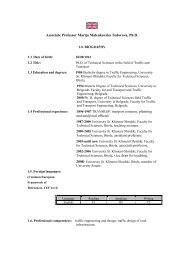
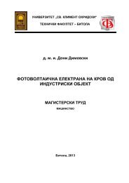
formation, inferencing, testing, validating, and refining. It is common practiceto start from a simple model and develop it in steps of increasing complexity,until it is capable of replicating the observed or anticipated behaviorof the real system to the extent that the modeler expects. It has to be kept inmind that all models need not be perfect replicates of the real system. If allthe details of the real system are included, the model can become unmanageableand be of very limited use. On the other hand, if significant and relevantdetails are omitted, the model will be incomplete and again be of limited use.While the scientific side of modeling involves the integration of knowledgeto build and solve the model, the artistic side involves the making of a sensiblecompromise and creating balance between two conflicting features of themodel: degree of detail, complexity, and realism on one hand, and the validityand utility value of the final model on the other.The overall approach in mathematical modeling is illustrated in Figure 2.1.Needless to say, each of these steps involves more detailed work and, as mentionedearlier, will include feedback, iteration, and refinement. In the followingsections, a logical approach to the model development process ispresented, identifying the various tasks involved in each of the steps. It is notthe intention here to propose this as the standard procedure for every modelerto follow in every situation; however, most of the important and crucial tasksare identified and included in the proposed procedure.ProblemformulationMathematicalrepresentationMathematicalanalysisInterpretationand evaluationof resultsFigure 2.1 Overall approach to mathematical modeling.© 2002 by CRC Press LLC

2.2.1 PROBLEM FORMULATIONAs in any other field of scientific study, formulation of the problem is thefirst step in the mathematical model development process. This step involvesthe following tasks:Task 1: establishing the goal of the modeling effort. Modeling projectsmay be launched for various reasons, such as those pointed out in Chapter 1.The scope of the modeling effort will be dictated by the objective(s) and theexpectation(s). Because the premise of the effort is for the model to be simplerthan the real system and at the same time be similar to it, one of theobjectives should be to establish the extent of correlation expected betweenmodel predictions and performance of the real system, which is often referredto as performance criteria. This is highly system specific and will also dependon the available resources such as the current knowledge about the systemand the tools available for completing the modeling process.It should also be noted that the same system might require different typesof models depending on the goal(s). For example, consider a lake into whicha pollutant is being discharged, where it undergoes a decay process at a rateestimated from empirical methods. If it is desired to determine the long-termconcentration of the pollutant in the lake or to do a sensitivity study on theestimated decay rate, a simple static model will suffice. On the other hand, ifit is desired to trace the temporal concentration profile due to a partial shutdownof the discharge into the lake, a dynamic model would be required. Iftoxicity of the pollutant is a key issue and, hence, if peak concentrations dueto inflow fluctuations are to be predicted, then a probabilistic approach mayhave to be adapted.Another consideration at this point would be to evaluate other preexisting“canned” models relating to the project at hand. They are advantageousbecause many would have been validated and/or accepted by regulators.Often, such models may not be applicable to the current problem with orwithout minor modifications due to the underlying assumptions about the system,the contaminants, the processes, the interactions, and other concerns.However, they can be valuable in guiding the modeler in developing a newmodel from the basics.Task 2: characterizing the system. In terms of the definitions presentedearlier, characterizing the system implies identifying and defining the system,its boundaries, and the significant and relevant variables and parameters. Themodeler should be able to establish how, when, where, and at what rate thesystem interacts with its surroundings; namely, provide data about the inflowrates and the outflow rates. Processes and reactions occurring inside the systemboundary should also be identified and quantified.Often, creating a schematic, graphic, or pictographic model of the system(a two-dimensional model) to visualize and identify the boundary and the© 2002 by CRC Press LLC

system-surroundings interactions can be a valuable aid in developing themathematical model. These aids may be called conceptual models and caninclude the model variables, such as the directions and the rates of flowscrossing the boundary, and parameters such as reaction and process ratesinside the system. Jorgensen (1994) presented a comprehensive summary of10 different types of such tools, giving examples and summarizing their characteristics,advantages, and disadvantages.Some of the recent software packages (to be illustrated later) have takenthis idea to new heights by devising the diagrams to be “live.” For example,in a simple block diagram, the boxes with interconnecting arrows can beencoded to act as reservoirs, with built-in mass balance equations. With thepassage of time, these blocks can “execute” the mass balance equation andcan even animate the amount of material inside the box as a function of time.Examples of such diagrams can be found throughout this book.Another very useful and important part of this task is to prepare a list ofall of the variables along with their fundamental dimensions (i.e., M, L, T )and the corresponding system of units to be used in the project. This can helpin checking the consistency among variables and among equations, in troubleshooting,and in determining the appropriateness of the results.Task 3: simplifying and idealizing the system. Based on the goals of themodeling effort, the system characteristics, and available resources, appropriateassumptions and approximations have to be made to simplify the system,making it amenable to modeling within the available resources. Again, theprimary goal is to be able to replicate or reproduce significant behaviors ofthe real system. This involves much experience and professional judgementand an overall appreciation of the efforts involved in modeling from start tofinish.For example, if the processes taking place in the system can be approximatedas first-order processes, the resulting equations and the solution procedurescan be considerably simpler. Similar benefits can be gained by makingassumptions: using average values instead of time-dependent values, usingestimated values rather than measured ones, using analytical approaches ratherthan numerical or probability-based analysis, considering equilibrium vs. nonequilibriumconditions, and using linear vs. nonlinear processes.2.2.2 MATHEMATICAL REPRESENTATIONThis is the most crucial step in the process, requiring in-depth subject matterexpertise. This step involves the following tasks:Task 1: identifying fundamental theories. Fundamental theories and principlesthat are known to be applicable to the system and that can help achieve thegoal have to be identified. If they are lacking, ad hoc or empirical relationships© 2002 by CRC Press LLC

may have to be included. Examples of fundamental theories and principlesinclude stoichiometry, conservation of mass, reaction theory, reactor theory,and transport mechanisms. A review of theories of environmental processesis included in Chapter 4. A review of engineered environmental systems ispresented in Chapter 5. And, a review of natural environmental systemsis presented in Chapter 6.Task 2: deriving relationships. The next step is to apply and integrate thetheories and principles to derive relationships between the variables of significanceand relevance. This essentially transforms the real system into amathematical representation. Several examples of derivations are included inthe following chapters.Task 3: standardizing relationships. Once the relationships are derived, thenext step is to reduce them to standard mathematical forms to take advantageof existing mathematical analyses for the standard mathematical formulations.This is normally done through standard mathematical manipulations, such assimplifying, transforming, normalizing, or forming dimensionless groups.The advantage of standardizing has been referred to earlier in Chapter 1with Equations (1.1) and (1.2) as examples. Once the calculus that applies tothe system has been identified, the analysis then follows rather routine procedures.(The term calculus is used here in the most classical sense, denotingformal structure of axioms, theorems, and procedures.) Such a calculusallows deductions about any situation that satisfies the axioms. Or, alternatively,if a model fulfills the axioms of a calculus, then the calculus can beused to predict or optimize the performance of the model. Mathematicianshave formalized several calculi, the most commonly used being differentialand integral. A review of the calculi commonly used in environmental systemsis included in Chapter 3, with examples throughout this book.2.2.3 MATHEMATICAL ANALYSISThe next step of analysis involves application of standard mathematicaltechniques and procedures to “solve” the model to obtain the desired results.The convenience of the mathematical representation is that the resultingmodel can be analyzed on its own, completely disregarding the real system,temporarily. The analysis is done according to the rules of mathematics, andthe system has nothing to do with that process. (In fact, any analyst can performthis task—subject matter expertise is not required.)The type of analysis to be used will be dictated by the relationships derivedin the previous step. Generalized analytical techniques can fall into algebraic,differential, or numerical categories. A review of selected analytical techniquescommonly used in modeling of environmental systems is included inChapter 3.© 2002 by CRC Press LLC

2.2.4 INTERPRETATION AND EVALUATION OF RESULTSIt is during this step that the iteration and model refinement process is carriedout. During the iterative process, performance of the model is comparedagainst the real system to ensure that the objectives are satisfactorily met.This process consists of two main tasks—calibration and validation.Task 1: calibrating the model. Even if the fundamental theorems and principlesused to build the model described the system truthfully, its performancemight deviate from the real system because of the inherent assumptionsand simplifications made in Task 3, Section 2.2.1 and the assumptions madein the mathematical analysis. These deviations can be minimized by calibratingthe model to more closely match the real system.In the calibration process, previously observed data from the real systemare used as a “training” set. The model is run repeatedly, adjusting the modelparameters by trial and error (within reasonable ranges) until its predictionsunder similar conditions match the training data set as per the goals and performancecriteria established in Section 2.2.1. If not for computer-based modeling,this process could be laborious and frustrating, especially if the modelincludes several parameters.An efficient way to calibrate a model is to perform preliminary sensitivityanalysis on model outputs to each parameter, one by one. This can identifythe parameters that are most sensitive, so that time and other resources can beallocated to those parameters in the calibration process. Some modern computermodeling software packages have sensitivity analysis as a built-in feature,which can further accelerate this step.If the model cannot be calibrated to be within acceptable limits, the modelershould backtrack and reevaluate the system characterization and/or themodel formulation steps. Fundamental theorems and principles as well as themodel formulation and their applicability to the system may have to be reexamined,assumptions may have to be checked, and variables may have to beevaluated and modified, if necessary. This iterative exercise is critical inestablishing the utility value of the model and the validity of its applications,such as in making predictions for the future.Task 2: validating the model. Unless a model is well calibrated and validated,its acceptability will remain limited and questionable. There are nostandard benchmarks for demonstrating the validity of models, because modelshave to be linked to the systems that they are designed to represent.Preliminary, informal validation of model performance can be conductedrelatively easily and cost-effectively. One way of checking overall performanceis to ensure that mass balance is maintained through each of the modelruns. Another approach is to set some of the parameters so that a closed algebraicsolution could be obtained by hand calculation; then, the model outputscan be compared against the hand calculations for consistency. For example,© 2002 by CRC Press LLC

y setting the reaction rate constant of a contaminant to zero, the model may beeasier to solve algebraically and the output may be more easily compared withthe case of a conservative substance, which may be readily obtained. Otherinformal validation tests can include running the model under a wide range ofparameters, input variables, boundary conditions, and initial values and thenplotting the model outputs as a function of space or time for visual interpretationand comparison with intuition, expectations, or similar case studies.For formal validation, a “testing” data set from the real system, either historicor generated expressly for validating the model, can be used as a benchmark.The calibrated model is run under conditions similar to those of thetesting set, and the results are compared against the testing set. A model canbe considered valid if the agreement between the two under various conditionsmeets the goal and performance criteria set forth in Section 2.2.1. Animportant point to note is that the testing set should be completely independentof, and different from, the training set.A common practice used to demonstrate validity is to generate a parity plotof predicted vs. observed data with associated statistics such as goodness offit. Another method is to compare the plots of predicted values and observeddata as a function of distance (in spatially varying systems) or of time (in temporallyvarying systems) and analyze the deviations. For example, the numberof turning points in the plots and maxima and/or minima of the plots andthe locations or times at which they occur in the two plots can be used as comparisoncriteria. Or, overall estimates of absolute error or relative error over arange of distance or time may be quantified and used as validation criterion.Murthy et al. (1990) have suggested an index J to quantify overall error indynamic, deterministic models relative to the real system under the sameinput u(t) over a period of time T. They suggest using the absolute error or therelative error to determine J, calculated as follows:J = T e(t) T e(t)dt or J = T ẽ(t) T ẽ(t)dtooe(t)where e(t) = y s (t) – y m (t) or ẽ(t) = y s(t)y s (t) = output observed from the real system as a function of time, ty m (t) = output predicted by the model as a function of time, t2.2.5 SUMMARY OF THE MATHEMATICAL MODELDEVELOPMENT PROCESSIn Chapter 1, physical modeling, empirical modeling, and mathematicalmodeling were alluded to as three approaches to modeling. However, as couldbe gathered from the above, they complement each other and are appliedtogether in practice to complete the modeling task. Empirical models are used© 2002 by CRC Press LLC

to fill in where scientific theories are nonexistent or too complex (e.g., nonlinear).Experimental or physical model results are used to develop empiricalmodels and calibrate and validate mathematical models.The steps and tasks described above are summarized schematically inFigure 2.2. This scheme illustrates the feedback and iterative nature of theprocess as described earlier. It also shows how the real system and the“abstract” mathematical system interact and how experimentation withthe real system and/or physical models is integrated with the modelingprocess. It is hoped that the above sections accented the science as well as theart in the craft of mathematical model building.Figure 2.2 Steps in mathematical modeling.© 2002 by CRC Press LLC

2.3 APPLICATION OF THE STEPS INMATHEMATICAL MODELINGIn this section, the application of the above steps in modeling the spatialvariation of a chemical in an advective-dispersive river is detailed. Becausethe focus of this book is on computer-based mathematical modeling usingauthoring software tools, the validation and calibration steps are only brieflyillustrated. It should not be construed in any way that they are of less importancein the modeling process. Other references must be consulted for furtherin-depth treatment of these steps.Step 1: Problem FormulationAn industry is proposing to discharge its waste stream containing a toxicantinto a nearby river. It is desired to set up discharge permits based on theimpact of the discharge on the water quality in the river. A preliminary modelhas to be developed to predict in-river concentrations of the toxicant under variousdischarge conditions and river flow rates under steady state conditions.Task 1: establishing a goal. The model has to replicate long-term, spatialvariations of the toxicant concentrations in the river. Because the real systemper se (river receiving the discharge) is not yet in existence, the desiredextent of correlation between the model and real system cannot be establishedin this case. However, let us pretend that from observations of similarsystems, the concentration profile can be expected to have cusp at the pointof discharge, with exponential-type decreases on either side. The modelshould be able to reproduce such a profile. It should enable the users to estimatein-stream concentrations up to 30 miles upstream and up to 50 milesdownstream and to determine the maximum discharge that can be allowedwithout violating certain water quality standards at the above two points. Adecision to build a detailed model will be made depending on the resultsfrom this preliminary model.Task 2: characterizing the system. The system in this case is the water column,enclosed for the most part by the physical boundaries provided by theriverbed and the banks. An imaginary cross-section at the upstream point ofinterest, A-A, and another imaginary section at the downstream point of interest,B-B, will complete the boundary as shown in Figure 2.3. The inflowcrosses the boundary at A-A, and the outflow crosses at B-B. The origin formeasuring distance along the river is taken as the point of discharge.The most significant variables in this problem can be identified as theflow rate in the river, the concentration of the toxicant in the inflow, the wasteinput rate, the reaction rate constants for the various processes that the toxicantcan undergo within the system, and the length of the river system. Othervariables can be the area of flow and the velocity of flow in the river. Some© 2002 by CRC Press LLC

Figure 2.3 Schematic of real system.of the environmental processes that the toxicant can undergo within the system,such as adsorption, desorption, volatilization, hydrolysis, photolysis,biodegradation, and biouptake, are illustrated in Figure 2.4.Task 3: simplifying the system. In general, the interactions between thetoxicant and the suspended solids and sediments can be under equilibrium,nonequilibrium, linear, or nonlinear conditions. The dissolved form of thetoxicant can undergo a variety of processes or reactions that can be of first orhigher order. The system parameters, such as area of cross-section and theflow rate of the river, etc., can vary spatially or temporally.Considering the project goals agreed upon and the physical, chemical, andbiological properties of the toxicant and the system, it may be reasonable tomake the following simplifying assumptions for the preliminary model:• Instantaneous mixing in the z- and y-directions occurs at the point ofdischarge; thus, the problem is reduced to a one-dimensional analysis.• Only the dissolved concentration of the toxicant is of significance andrelevance; thus, interactions with sediments through suspended solidsare negligible.• All reactions undergone by the toxicant are of first order; thus, all theindividual reaction rate constants, k i , can be lumped to an overall rateconstant, K = Σ k i .• The river is of fixed prismatic section; thus, the area of flow is timeinvariantand space-invariant within the system boundary.• The dispersion coefficient is significant only in the x-direction andremains constant within the system boundary.• The flow rate is an average constant value, but can be changed, viz.,a parameter.© 2002 by CRC Press LLC

VolatilizationHydrolysisPhotolysisBiodegradationDissolved formof toxicantDiffusionAdsorptionDesorptionBiouptakeDepurationSedimentsSuspendedsolidsScourSettlingFigure 2.4 Environmental processes acting upon dissolved toxicant.• The river flow and waste input are the only inflows into the system,and the river flow is the only outflow from the system.• The volumetric flow of the waste stream is negligible compared to theriver flow.With these assumptions, the system is reduced to a simplified form as shownin Figure 2.5. The variables of significance and relevance are listed in Table2.1 along with their respective symbols, dimensions, and common units.Figure 2.5 Schematic of the simplified system.© 2002 by CRC Press LLC

Table 2.1 Variables, Symbols, Dimensions, and UnitsVariable Symbol Dimension UnitRiver flow rate Q L 3 T 3 cfsConcentration of toxicant C ML –3 mg/LFirst-order reaction rate constant k T –1 1/dayArea of flow A L 2 sq ftVelocity of flow U LT –1 ft/sDispersion coefficient E L 2 T –1 sq miles/dayLength in direction of flow x L milesTime t T dayStep 2: Mathematical RepresentationTask 1: identifying fundamental theories. Having simplified the system,the appropriate fundamental theorems, laws, and principles necessary to buildthe model to achieve the goal can be identified as follows:• Toxicant mass balance based on conservation of mass:Rate of changeof mass oftoxicant insidesystemNet rate of Net rate of Net rate ofadvective diffusive loss of= + – (2.1)inflow of inflow of toxicant duetoxicant toxicant to reactions• Advective mass flow rate based on continuity:= [river flow rate, Q] × [concentration of toxicant, C] (2.2)• Dispersive mass flow rate based on Fick’s Law:= [dispersion coefficient, E] × [area of flow, A]× [concentration gradient, ∂C/∂x] (2.3)• Mass loss due to reaction based on first-order reaction kinetics:= [reaction rate constant, k] × [volume, V] × [concentration, C] (2.4)If other processes, such as interactions with suspended solids, bioaccumulation,volatilization, etc., are to be included, then appropriate principles andrelationships have to be included in this listing.Task 2: deriving relationships. The fundamentals identified in Task 2 cannow be combined to derive an expression for the output(s). This involves© 2002 by CRC Press LLC

standard mathematical manipulations such as simplification, substitution,and rearrangement.In this example, a distributed model is appropriate because of spatial variationsof the output. The calculi of “differential calculus” is applied to derivethe governing partial differential equation. The fundamentals identified aboveare applied to a small element of length, ∆x, within the system over an infinitesimaltime interval, ∆t, as illustrated in Figure 2.6.The components of the mass balance equation for the toxicant can beexpressed in terms of the symbols as follows:Rate of change of mass of toxicant within the element = ∂(V C) (2.5)∂tAdvective inflow rate into element = QC (2.6)Advective outflow rate from element = QC + ∂( QC)∆x∂x(2.7)∴ Net advective inflow = QC – QC + ∂( Q∂∆x C) x= – ∂( QC)∂ ∆xfrom elementx(2.8)Diffusive inflow rate into element = –EA ∂ C∂x(2.9)Diffusive outflow rate from element = –EA ∂ C ∂ + ∂x∂ x –EA ∂ C∂x∆x (2.10)InflowsReaction lossAdvectiveAdvectiveOutflowsDispersiveDispersive∆xFigure 2.6 Detail of element.© 2002 by CRC Press LLC

∴Net diffusive inflow = –EA ∂ C∂x– –EA ∂ C ∂ + ∂x∂ x –EA ∂ Cinto element∂x∂= EA ∂ x ∂ C∂x∆x ∆x (2.11)Net rate of loss of toxicant due to reactionswithin the element = k(A∆x)C (2.12)Combining the above expressions now completes the mass balance equation: ∂(V C) = – ∂( QC)∂∆x + ∂t ∂x∂ x EA ∂ C∂x∆x – k(A∆x)C (2.13)The solution to the above partial differential equation will yield the output Cas a function of time, t, and distance, x.Based on the goals and the assumptions, the model has to describe steadystate conditions, and temporal variations are not required; hence, the partialderivative term on the left-hand side (LHS) of the above equation equals zero,and the equation becomes an ordinary differential equation. Further, Q is aconstant, but a parameter; E and A are assumed constant within the boundary;thus, the above equation reduces to the following:20 = –Q d C∆x + EA d Cdxdx2∆x – k(A∆x)C (2.14)which on division by (A∆x) simplifies further to:20 = – Q A d C + E d Cdxdx2 – kC (2.15)Task 3: standardizing relationships. The relationship(s) derived from thefundamental theories and principles can now be translated into standardmathematical forms for further manipulation, analysis, and solving. Mathematicalhandbooks containing solutions to standard formulations have to bereferred to in order to identify the ones matching the equations derived.In this example, the final equation can be recognized as a second-order,ordinary, homogeneous, linear differential equation, of the standard form:whose solution can be found from handbooks as:0 = ay by cy (2.16)y Me gx Ne jx (2.17)© 2002 by CRC Press LLC

where g and j are, in turn, the positive and negative values of –b ±b c/2a,2 – 4aand M and N are constants to be found from two boundary conditions.Step 3: Mathematical AnalysisComparing the coefficients of the final equation derived in our examplewith those of the standard equation, a = E, b = –(Q/A), and c = –K.Recognizing that Q/A = U, the river velocity, b = –U. Thus, g and j are firstfound as follows:g, j U ± U2 +4Ek U = (1 ± α) (2.18)2E2 Ewhere, α = 1 + 4 Ek2U (2.19)Now, the constants M and N have to be determined using appropriate boundaryconditions for this particular situation. (This is another reason for establishingthe system boundary in advance.) It is convenient in this case toconsider the reaches upstream and downstream of the discharge point as twoseparate regions to determine the boundary conditions (BCs). Assuming thetoxicant concentration far upstream and far downstream from the dischargepoint will approach near-zero values, the following boundary BCs can beused to find M and N and, hence, the final solution:Upstream reach: x ≤ 0BC 1: x = 0, C = C 0BC 2: x = –∞, C = 0M = C 0N = 0and,C = C 0 e gxDownstream reach: x ≥ 0BC 1: x = 0, C = C 0BC 2: x = +∞, C = 0N = C 0M = 0and,C = C 0 e jxIt remains to determine C 0 to complete the solution. A mass balance acrossan infinitesimal element at the discharge point can now yield the value for C 0© 2002 by CRC Press LLC

in terms of the model parameters already defined. This element can be treatedas a subsystem at the discharge point as shown in Figure 2.7.The mass inflow, outflow, and reaction loss for this element are as follows:CMass inflow into element = QC 0 – EA d dxx(2.20)=0–εCMass outflow from element = QC 0 – EA d dxx(2.21)=0+εReaction loss within element = kCA∆x = 0Hence, the mass balance equation for the element, ignoring the reaction lossin the infinitesimal element, is as follows:CCQC 0 – EA d dxx+ W = QC 0 – EA d =0–ε dxx(2.22)=0+εNow, substituting from the previous expressions for C,and simplifying,or,–EA d[C 0e gxd ]x+ W = –EA 0ex [C =0–ε d x x(2.23)=0+ε–EAC 0 g W = –EAC 0 j (2.24)jx ]WC 0 = (2.25)EA( g – j)Input oftoxicant, ,WxFigure 2.7 Element at point of discharge.© 2002 by CRC Press LLC

On substituting for g and j from the above, C 0 = W/αQ, where W is the massrate of discharge into the river. The final model for this problem is, therefore:Step 4: Interpretation of ResultsC = αWQ e gx for x ≤ 0 (2.26)C = αWQ e jx for x ≥ 0 (2.27)The calibration and validation of the model will be highly problemspecific.Initial interpretations can include simulations, sensitivity analysis,and comparison with other similar systems. As a first step in this case, themodel can be run with typical parameters and known inputs. The output canbe used to corroborate the performance of the model against intuition, pastexperience, or literature results to verify that the model outputs generally followthe observed profiles and are within reasonable ranges. Because the resultin this case is a function of x rather than a numerical value, it may be usefulto plot the variation of C as a function of x to check if the model is reflectingthe spatial concentration profile.As an example of calibration and validation, let us use an artificial data set(adapted from Thomann and Mueller, 1987):Distance (mi) –15 –10 –5 0 5 10 15Concentration (mg/L) 0.43 1.22 3.50 10.00 4.49 2.02 0.91This data set had been collected on an estuary flowing at 100 cfs with an averagecross-sectional area of 10 × 10 5 sq ft, receiving a waste input of 372,000lbs/day at 0 miles. The decay rate of the waste material was measured to be0.1 day –1 . The dispersion for this estuary was estimated to be in the range of2–5 sq miles/day.As a first step, an appropriate value for the dispersion coefficient, E, hasto be established. The data from the upstream portion of the estuary are usedto calibrate the model to fit the four data points by running the model withvarious values of E ranging from 2 to 5 sq miles/day. Given the value of E,the remaining three data points may be used to validate the model. These considerationsare illustrated in Figure 2.8, from which the value of E can be estimatedto be 3 sq miles/day. With this value for E, the model is capable offitting the upstream data points as well as predicting the downstream datapoints. While acknowledging that the validation and calibration exercise inthis example is somewhat academic, the very same procedure is used in practiceto calibrate and validate mathematical models.© 2002 by CRC Press LLC

Figure 2.8 Model predictions vs. measured data.The value of the simplifying assumptions made at the beginning of theanalysis is in the reduction of the governing equation to a form amenable toa closed solution. Such an analysis provides highly useful insight and acts asa stepping stone for the modeler to gradually add pertinent details andrefinements to build more realistic models. Needless to say, as the modelsbecome more detailed and realistic, analytical methods of solving the governingequations can be extremely complicated or impossible. In such cases,using computer-based, numerical approaches is the only way to complete themodeling process. In the next chapter, some of the common analytical andnumerical approaches used in environmental modeling efforts will be reviewed.© 2002 by CRC Press LLC

CHAPTER 3Primer on MathematicsCHAPTER PREVIEWThis chapter contains a review of mathematical methods and tools asthey apply to environmental modeling. It is assumed that the readershave taken a formal sequence of college-level course work in mathematicsleading up to partial differential equations. In the first part ofthis chapter, reviews of different types of mathematical formulationsare summarized. Analytical and numerical procedures for solving themare outlined. Then, ways to implement some of the more common proceduresin the computer environment are demonstrated.3.1 MATHEMATICAL FORMULATIONSIN the previous chapter, several steps and tasks involved in the model developmentprocess were identified. It goes without saying that a clear understandingof mathematical formulations and analyses is a necessary prerequisitein this process. A strong mathematical foundation is required to transmutesubject matter knowledge into mathematical forms such as functions, expressions,and equations. Knowledge of analytical procedures in mathematicalcalculi such as simplifying, transforming, and solving, is essential to selectand develop the appropriate computational procedures for computer implementation.The selection of an appropriate computer software package tocomplete the model also requires a good understanding of the mathematicsunderlying the model. As pointed out in Chapter 1, different formulations canbe developed to describe the same system; hence, the ability to choose theoptimal one that can meet the goals requires a strong mathematical foundation.The advantage of reducing the formulations to standard mathematicalforms has been pointed out before. For modeling purposes, a wide variety ofenvironmental systems can be categorized as deterministic with continuous© 2002 by CRC Press LLC

variables. Deterministic systems can be described either by static or dynamicformulations. This chapter will, therefore, focus on the mathematical calculifor continuous, deterministic, static, and dynamic systems with up to fourindependent variables. Brief discussions of how these deterministic modelscan be adapted for probability systems will be illustrated in selected cases inlater chapters. In the following sections, selected standard mathematical formulationscommonly encountered in modeling environmental systems arereviewed. In a broad sense, these formulations can be classified as eitherstatic or dynamic.3.1.1 STATIC FORMULATIONSStatic models are often built of algebraic equations. The general standardform of the algebraic equation in static formulations is as follows:G(x,y,) = 0 (3.1)where G is a vector function, x and y are vector variables, and θ is a set ofparameters. In the context of a model, x can correspond to the inputs, y theoutputs, and θ the system parameters. If x and y are linear in G, the model iscalled linear, otherwise, it is nonlinear.3.1.2 DYNAMIC FORMULATIONSDynamic systems with continuous variables are normally described by differentialequations. Any equation containing one or more derivatives is calleda differential equation. When the number of independent variables in a differentialequation is not more than 1, the equation is called an ordinarydifferential equation (ODE), otherwise, it is called a partial differential equations(PDE).The general standard form of an ODE is as follows:n z2 zn– 1α(t) d ( t)ndt = Gz(t), dz (d , t)t d ( t)d 2t, ... d z(t)d n–1t, u(t), du ( t)d ,t d2 u(t), . . . , (t)2dt(3.2)where u(t) is a known function, α(t) and θ(t) are parameters, and z(t) is thedependent variable. In the context of a model, t can correspond to time, u tothe input, z the output, and α(t) and θ(t) the system parameters.An ODE is ranked as of order n if the highest derivative of the dependentvariable is of order n. When α(t) is nonzero, i.e., the equation is nonsingular,© 2002 by CRC Press LLC

it can be simplified by dividing throughout by α(t). Often, in many environmentalsystems, θ(t) does not change with t. Further, if G is linear in z(t), u(t),and their derivatives, then the equation is linear, and the principle of superpositioningcan be applied.The general standard form of a PDE with two independent variables x andt is as follows:whereG[u, u x , u t , u xx , u xt , u tt , (x,t), f(x,t)] = 0 (3.3)2u x = ∂ u; u t = ∂ u; u xx = ∂ u∂x∂t∂t2; u xt = ∂ u∂t2; u tt = ∂ u∂t2, (x,t)is a parameter and f(x,t) is a known function. In the context of a model, x cancorrespond to a spatial coordinate, t to time, f(x,t) to the input, θ(x,t) to thesystem parameter, and u(x,t) to the system outputs. The formulation shouldalso define the problem domain, i.e., ranges for x and t.223.2 MATHEMATICAL ANALYSISSome of the formulations identified above are tractable to an analyticalmethod of analysis, while many require a computational (also referred to asnumerical) method of analysis. Both methods of analysis can form the basisof computer-based mathematical modeling.3.2.1 ANALYTICAL METHODSIn analytical methods, the solution to a formulation is found as an expressionconsisting of the parameters and the independent variables in terms ofthe symbols. Sometimes this method of solution is referred to as parameterizedsolutions. The solution can be exact or approximate. Only for a limitedclass of formulations is it possible to find an exact analytical solution. Anapproximate solution has to be sought in other cases, such as in the modelsfor large environmental systems.For example, consider Equation (3.1), where y is the unknown, x is aknown variable, and θ is a parameter. The solution for y might or might notexist; if it does, it might not be unique. If Equation (3.1) could be rearrangedto the formA(x,)y B(x,) = 0 (3.4)a solution can be found by inverting the matrix A(x,θ) if and only if A(x,θ) isa nonsingular n × n matrix. If y appears nonlinearly, multiple solutions may© 2002 by CRC Press LLC

e possible, and a computational method of analysis would be necessary tofind them.3.2.2 COMPUTATIONAL METHODSIn this method, the solution is found numerically, often with the aid of acomputer. The solutions in this case are only approximate, and numeric.Therefore, the formulation should include numeric values for the modelparameters and variables, whereas symbolic representations will suffice in thecase of the analytical method of analysis. The advantage of the computationalmethod of analysis is that it can be applied to a much wider class of mathematicalformulations, particularly for complex systems.It is not within the scope of this book to identify all the standard mathematicalcalculi and procedures for analyses, rather, some specific examplesof analyses pertaining to typical environmental systems are illustrated. Theintent of this illustration is for the readers to be able to adapt them for implementationin the computer environment.3.3 EXAMPLES OF ANALYTICAL ANDCOMPUTATIONAL METHODSThe governing equations in environmental models may be reduced to simplealgebraic equations (e.g., steady state concentration of a contaminant in acompletely mixed lake), systems of simultaneous linear equations (e.g., steadystate concentrations in completely mixed lakes in series), ODEs (e.g., transientconcentration in a well-mixed lake), systems of ODEs (e.g., biomass growth,substrate consumption, and oxygen level in a completely mixed lake), or PDEs(e.g., contaminant transport in a stratified lake under transient loads). In thissection, common algorithms for solving these types of formulations are outlined.Many of these algorithms can be implemented in spreadsheet programswith minimal syntax or programming. Many standard algorithms are includedas preprogrammed libraries in other software packages discussed in thisbook. Some examples of implementations are included in this chapter to illustratethe general approach, and more detailed ones for specific problems canbe found in Chapters 8 and 9.3.3.1 ALGEBRAIC EQUATIONS3.3.1.1 Classifications of Algebraic EquationsThe most general form of the algebraic equation was given in Equation(3.1), and a solvable form was provided in Equation (3.4). Considering a© 2002 by CRC Press LLC

Algebraic equationsLinear equationsNonlinear equationsOne Multiple One Multipleequation equations equation equationsOne One Polynomial Transcendental Multiplesolution solution set equation equation solution setsNº of solutions equalsdegree of polynomialUnspecified numberof solutionsFigure 3.1 Classification of algebraic equations.simpler form of G, such as f(x) = 0, its solution or “root” is the value of theindependent variable, x, that when substituted into f(x) will make it equal tozero. Methods to find those roots for such equations depend on the number ofequations and the type of equations to be solved. Classification of algebraicequations is shown in Figure 3.1 to help in this selection process.3.3.1.2 Single, Linear EquationsAnalytical methods of elementary algebra for solving single, linear equationsfor one unknown are rather straightforward and are not discussed further.3.3.1.3 Set of Linear EquationsSimultaneous linear equations are frequently encountered in environmentalmodeling. Typical examples include chemical speciation calculations andnumerical solution of partial differential equations. A general form of a set ofm linear equations with n unknowns is Ax = B, where A is a given m × nmatrix, and B is a given vector. The solution is given by x = A –1 B. This equationin general will have a unique solution only if m = n; if m < n, infinitelymany solutions may be possible; and if m > n no solutions are possible. Anexample of a set of linear simultaneous equations is as follows:a 11 x 1 a 12 x 2 a 13 x 3 b 1a 21 x 1 a 22 x 2 a 23 x 3 b 2a 31 x 1 a 32 x 2 a 33 x 3 b 3© 2002 by CRC Press LLC

or, in matrix forma 11 a 12 a 13a 21 a 22 a 23a 31 a 32 a 33x 1 b 1 x b 2 2x 3b 3where a ij are the coefficients, b’s are constants, and x’s are the unknowns.The Gauss-Seidel iterative method is a convenient computational methodused for solving such a set of equations. The algorithm first solves the firstequation for x 1 , the second for x 2 , and the third for x 3 .x 1 = b 1 – a 12 x2– a 13 x 3a11x 2 = b 2 – a 21 x1– a 23 x 3a22(3.5a)(3.5b)x 3 = b 3 – a 31 x1– a 32 x 2a33(3.5c)The process is iterated with resubstitution, until a desired degree of convergenceis reached using Equations (3.5). This algorithm is illustrated in thenext example.Worked Example 3.1Solve the following simultaneous equations:Solution4 X1 + 6 X2 + 2 X3 = 112 X1 + 6 X2 + X3 = 213 X1 + 2 X2 + 5 X3 = 75Figure 3.2 shows an Excel ®3 implementation for solving the three equations,which are entered in rows 2 to 4. Note how the coefficients are enteredinto separate cells so that they can be referred to by cell reference. The Gauss-Seidel algorithm is entered into rows 6 to 8, in column N, to estimate X1, X2,and X3, respectively.For illustration, the algorithm is expressed in Excel ® language in columnL, against each X row. Notice that the formula in cell L6 refers to cell L7,while the formula in cell L7 refers back to L6. This is known as circular3 Excel ® is a registered trademark of Microsoft Corporation. All rights reserved.© 2002 by CRC Press LLC

Figure 3.2 Gauss-Siedel algorithm implemented in the Excel ® spreadsheet program.reference in Excel ® and will cause an error message to be generated. To executesuch circular references, the Iteration option in the Calculation panelunder the Preferences menu item under the Tools menu should be turned on.Once the equations are entered, the spreadsheet can be Run to solve the equationsiteratively. The results calculated are returned in column N. Finally, theresults can be checked by feeding them back into the original equations toensure that they satisfy them as shown in rows 10 to 12.Other methods such as the Gauss Elimination method are also availableto solve linear simultaneous equations. Most equation solver-based packagesfeature built-in procedures for solving these equations, requiring minimalprogramming.An example of the use of Excel ® ’s built-in Solver utility that can be usedto solve a set of equations is presented next. Consider the same set of equationssolved in Worked Example 3.1, and let the functions f, g, and h representthose equations:f ≡ 4 X1 + 6 X2 + 2 X3 – 11g ≡ 2 X1 + 6 X2 + X3 – 21h ≡ 3 X1 + 2 X2 + 5 X3 – 75Recognizing the fact that the roots of the above equations will make y = f 2 +g 2 + h 2 = 0, the problem of finding those roots can be tackled readily by callingthe Solver routine of Excel ® as illustrated in Figure 3.3. Here, X1, X2, andX3 are assigned arbitrary guess values of 1, 2, and 3 in column M. The expressionfor y is entered into cell J6. The Solver routine is selected from the Toolsmenu, and the target cell and the cells to be changed are specified in theSolver Parameter dialog box. The routine then will find the values of X1, X2,and X3 that will make y = 0.© 2002 by CRC Press LLC

(a)(b)Figure 3.3 (a) Setting up Solver routine in Excel ® ; (b) results from Solver routine.As an alternate approach, equation solver-based packages that have builtinroutines for solving simultaneous equations can be used. For example, theMathematica ®4 equation solver-based software can be used as shown inFigure 3.4. The coefficients a ij and b k are first assigned appropriate numericalvalues. Then, the built-in routine, Solve, is called with two lists of arguments.The first list contains all the equations to be solved in symbolic form,and the second list contains the variables for which the equations are to besolved. When executed, the roots of the three equations are returned in lineOut[1] as x1 = –16.381; x2 = 5.16667; and x3 = 22.7619.An elegant way to solve a set of linear equations is by following the mathematicalcalculi of matrix algebra. Another equation solver-type software4 Mathematica ® is a registered trademark of Wolfram Research, Inc. All rights reserved.© 2002 by CRC Press LLC

Figure 3.4 Using Mathematica ® for solving simultaneous equations.package, MATLAB ®5 , allows this to be set up effortlessly. The same set ofequations as in the above example is solved in MATLAB ® as shown in Figure3.5. The matrix a is first specified with a ij , followed by matrix b with b’s.Then, by entering the command x = b/a, MATLAB ® returns the solution forx with x1 = –16.3810; x2 = 5.1667; and x3 = 22.7619.3.3.1.4 Single, Nonlinear EquationsThe next class of algebraic equations is single, nonlinear equations.Solution methods for nonlinear equations are either direct or indirect. In thedirect method, known formulas are applied to standard forms of the equationsin a nonrepetitive manner (analytical methods of analysis). A typical exampleis the standard solution for a second-order polynomial equation, otherwiseknown as the “quadratic equation”: ax 2 + bx + c = 0, whose roots are givenby {–b ± bc}/2a.2 – 4aSuch formulas are not readily available or unknown for many types of equations.Hence, indirect methods have to be used in those cases. In the indirectmethod, repeated application of some algorithm is implemented to yield anapproximate solution (computational method of analysis). The indirect methodsare the ones that are utilized in computer modeling of complex systems.Nonlinear equations can be either polynomial or transcendental. The computationalmethods for solving such equations start with a guessed value forthe root and follow standard computer algorithms to systematically refine thatguess in an iterative manner until the equation is satisfied within acceptablelimits. Two simple methods are outlined here.In the first, known as the binary method, two guesses x I and x u are madesuch that they bracket the real root, x: x I < x and x u > x. While this may appearcircuitous, as x is not known, x I and x u can be found rather easily by taking5 MATLAB ® is a registered trademark of The MathWorks, Inc. All rights reserved.© 2002 by CRC Press LLC

Figure 3.5 Using MATLAB ® for solving simultaneous equations.advantage of the fact that the function should change sign within the intervalbounded by x I and x u . Or, in other words, guess x I and x u so that:f (x I ,) • f (x u ,) < 0 (3.6)This can be readily achieved by plotting the function. Then, a refined valueof the root, x r , can be estimated as = ( x I + x u )/2. To make the next refinedguess, a new bracket is now defined with either x I and x r or x r and x u . Again,a sign change of f (x) is used to decide which range to make the new guessfrom:if f (x I ,) × f (x r ,) < 0, the new guess is made between x I and x rif f (x r ,) × f (x u ,) < 0, the new guess is made between x r and x u(3.7a)(3.7b)This process is iterated until the new guess is not significantly different fromthe previous one; at that point, the root is taken as the value of the last guess.Worked Example 3.2First-order processes occurring in many environmental systems can bedescribed by the equation: C = C 0 e –kt , where C is the concentration of thechemical undergoing the reaction, C 0 is its initial concentration, k is the reactionrate constant, and t is the time. Find the time it would take for the concentrationto drop from 100 mg/L to 10 mg/L.SolutionEven though the equation can be solved for t algebraically, the binarymethod is used here to illustrate the method and to compare its performanceagainst the direct algebraic solution. The algebraic solution can be readilyseen as t = 9.21. The implementation of the binary algorithm in an Excel ®spreadsheet is shown in Figure 3.6.© 2002 by CRC Press LLC

Figure 3.6 Implementation of binary method in Excel ® spreadsheet.The first step in the binary method is to guess the lower and upper boundsof the root by calculating the function C – C 0 e –kt for a range of values of t todetermine the value of t at which a sign change occurs. It can be readily donein Excel ® by entering the function in cell C12 and filling it down, with t valuesset up in column B, again by filling down. The upper and lower boundsare seen to be t = 9 and t = 10. The following algorithms, based on Equation(3.5), are entered into cells F15 and G15, and filled down to perform the calculationsautomatically for seven steps, in this case:Cell F15:Cell G15:IF(($C$4-Co*EXP(-k*F14))*($C$4-Co*EXP(-k*H14))

Another method, known as the Newton-Raphson method, requires onlyone guess to start the iterative process. It is based on Taylor’s expansion ofthe form:f (x n h) f (x n1 ) f (x n ) hf(x n ) h f(x n ) + . . . (3.8)22If h 2 and higher terms are ignored, it can be seen that the step from x n to x n+1moves the function value closer to a root so that f (x n h) = 0. Then,x n1 x n – f ( xn) (3.9)f(x )Here, the computational process starts with a guess value for x n . Then, usingf (x n ) and f(x n ), a value for x n1 is calculated. If f (x n1 ) is sufficiently small,the root is taken as x n1 ; or, a new value for x n1 is calculated using the currentvalue of x n1 for x n in Equation (3.7), and the process is repeated. Amodification to this method is the Secant method, which is preferable whenit is difficult to get the derivative f(x n ) to be used in Equation (3.7). In suchcases, the Secant method uses the following approximation for f(x n ):nf (x n ) ≈ slope at x n f(x n)–f(xn–1) (3.10)x – xEven though these methods can be implemented in a spreadsheet with relativeease, most equation solver-based software packages feature built-infunctions that can return the solutions to such equations more efficiently andaccurately, without requiring any programming. Spreadsheet packages suchas Excel ® also include some built-in functions that are preprogrammed to performiterative calculations for solving simple equations.The use of the built-in Goal Seek feature of Excel ® in solving the problemin Worked Example 3.2 is illustrated in Figure 3.7. In this worksheet, theright-hand side of the equation to be solved is entered in cell C4. Then, theGoal Seek option is selected from the Tools menu. To start the Goal Seekprocess, cell C4 is specified to be 10 by changing the value of cell C6. Theprocess is instantly executed, and the result is returned as 9.21014.Alternatively, in equation solver-based software packages, such equationscan be solved readily by calling appropriate built-in routines. For example,Figure 3.8 shows how the above problem can be solved in Mathematica ® . Thevariables in the equation are defined first. The built-in routine Solve is calledwhere the first argument contains the equation to be solved. The secondargument is the variable for which the equation is to be solved. When executed,the solution is returned in line Out[2] as 9.21034. Note that theMathematica ® sheet is set up so that one can change the values of the variablesand readily solve the equation for t. In addition, the same setup can beused to solve for any one of the four variables in the equation, provided thenn–1© 2002 by CRC Press LLC

Figure 3.7 Using Goal Seek function in Excel ® for solving nonlinear equations.Figure 3.8 Using Mathematica ® to solve nonlinear equations.other three are known. This is achieved by specifying the unknown variableto solve for as the second argument to the call to Solve.3.3.1.5 Set of Nonlinear EquationsThe general form of a set of nonlinear equations can consist of n functionsin terms of n unknown variables, x i :f 1 (x 1 , x 2 , . . . x n ) 0; f 2 (x 1 , x 2 , . . . x n ) = 0; . . . .© 2002 by CRC Press LLC

and so on up tof n (x 1 , x 2 , . . . x n ) = 0 (3.11)There are no direct methods for solving simultaneous nonlinear equations.The most popular method for solving nonlinear equations is the Newton’sIteration Method, which is based on Taylor’s expansion of each of the nequations. For example, the first of the above equations can be expressedas follows:∂f f 1 (x 1 ∆x 1 , . . . x n ∆x n ) = f 1 (x 1 , . . . x n ) 1 ∂x ∆x 11+ higher-order terms (3.12)Neglecting higher-order terms,∂f 1 (x 1 ∆x 1 , . . . x n ∆x n ) = f 1 (x 1 , . . . x n ) ∂x ∆x (3.13)1If, from a guessed value of x1, the change ∆x1 would make the left-handside approach 0, then the true root will be x1 ∆x1. Or, in other words, if ∂∂x ∆x = –f (x , . . . x ) (3.14)1 1 1 nf 11then x 1 ∆x 1 will be a root. Thus, extending this argument to the set of equations,this algorithm reduces to the solution of a set of linear equations thatcan be represented in the following form:⎡ ∂f⎢⎢∂x⎢⎢ ∂f⎢∂x⎢⎢∂f⎢⎣⎢∂x1121∂f∂x∂f∂x∂f∂x∂f1⎤⎥∂xn⎥⎥∂f2⎥∂x⎥⎥∂f⎥⎥∂xn⎦⎥n n nf 11(3.15)The algorithms discussed in the previous section for a set of linear equationscan now be applied to the above set of linear equations to find their roots.3.3.2 ORDINARY DIFFERENTIAL EQUATIONS12221 2. . .. . .. . .A vast majority of environmental systems can be described by ODEs. Onlyin a limited number of such cases can these equations be solved analytically,n⎡∆x1⎢⎢∆x2⎢⎢ .⎢⎢ .⎢⎢⎣∆xn⎤⎥⎥⎥⎥⎥⎥⎥⎥⎦⎡−f1⎤⎢ ⎥⎢−f2⎥⎢ ⎥= ⎢ . ⎥⎢ ⎥⎢ . ⎥⎢ ⎥⎢⎣−f ⎥n ⎦© 2002 by CRC Press LLC

whereas all of them can be readily solved using computational methods.Whichever method is used, the solution of ODEs requires that the dependentvariable and/or its derivatives be known constraints at prescribed values of theindependent variable. When all of these known constraints are at zero valueof the independent variable, the problem is called an “initial value problem.”In other cases, where the constraints are known at nonzero values of the independentvariable, the problem is called a “boundary value problem.” The constraintsin the two cases are known as “initial conditions” (ICs) and“boundary conditions” (BCs), respectively. It has to be noted that the solutionto a differential equation should satisfy the equation and the initial or boundaryconditions.3.3.2.1 Analytical Solutions of ODEsThe general form of an ODE may be stated as follows: d y = f (x,y)dxwith an IC ofy(x 0 ) = y 0 (3.16)The solution to this will be a function y(x) that satisfies both the differentialequation and the IC. Analytical solutions for some of the more common functionsf (x,y) and ICs are summarized here. Additional solutions can be foundin mathematical handbooks.a. First-order equations: when an ODE can be expressed in the form:M(x)dx + N(y)dy = 0then the equation is separable, and the solution can be found by integratingeach term in:∫M(x)dx = –∫N(y)dy (3.17)b. First-order nonhomogeneous linear equations: when an ODE can beexpressed in the form: d y P(x)y = Q(x)dxit can be solved by using an integrating factor of the form: e∫P(x)dx togive the solution aswhere b is a constant of integration.∫{e ∫P(x)dx Q(x)}dx by = (3.18)e∫P(x)dx© 2002 by CRC Press LLC

c. Second-order equation with equidimensional coefficients: when the ODEcan be expressed in the form:2 y d dx2 a x d y dxxb2 y = 0a trial solution of the form y = cx s , where s is found from:(a – 1) ± (a – 1)s = – 2 – 4b(3.19)2giving the solution asy = b 1 x s1 + b 2 x s2 if s1 ≠ s2 (3.20a)y = b 1 x s + b 2 x s ln x if s1 = s2 = s (3.20b)d. Second-order equation with constant coefficients: when the ODE can beexpressed in the form:2 y d dx2 a d y by = 0dxa trial solution of the form y = be sx , where s is found from:giving the solution asWorked Example 3.3a ± as = – 2 – 4b (3.21)2y = b 1 e s1x + b 2 e s2x if s1 ≠ s2 (3.22a)y = b 1 e sx + b 2 xe sx if s1 = s2 = s (3.22b)The buildup of the concentration, C, in a lake due to a new step waste loadinput can be described by the following equation (to be derived in Chapter 6): d C 1.23C = 2.0dtThe initial concentration of the waste material in the lake = 0. Develop a solutionto the above ODE to describe the concentration in the lake as a functionof time.© 2002 by CRC Press LLC

SolutionThe solution can be found by first categorizing the ODE and then followingstandard appropriate mathematical calculi. Alternatively, some computersoftware packages can find the analytical solution directly. The two approachesare illustrated in this example.The given equation can be seen as a special case of a first-order nonhomogeneouslinear equation identified earlier, with y = C, x = t, P(x) = 1.23,and Q(x) = 2.0. It can, therefore, be solved by applying Equation (3.18):Integrating factor = ≡ e ∫P(t)dt ≡ e ∫1.23dt = e 1.23tHence, the solution to ODE is as follows:2 1. 23 {e1.23t } b∫{e 1.23t 2}dt bC = = e 1.23 e1.23tt2= 1. 23 1 1. 232 be –1.23t From the initial condition given, C = 0 at t = 0; therefore, b = – 1.223 Thus, the final solution for C as a function of t is as follows:C 1.223 {1 – e–1.23t } 1.63{1 – e –1.23t }See Worked Example 3.4 for a plot of the above result.As an alternate approach, an equation solver-based software package,Mathematica ® , is used to find the solution directly as shown in Figure 3.9.Here, the built-in procedure, DSolve, is called in line In[1] with the followingarguments: the ODE to be solved, the initial condition, the dependentvariable, and the independent variable. The solution is returned in line Out[2],with the integration constant automatically evaluated, by Mathematica ® .Finally, the Plot function is called to plot the solution showing the variationof C with t.It can be seen that the solution returned by Mathematica ® in line Out[2],after some manipulation, is identical to the solution found earlier by followingthe standard mathematical calculi. This example illustrates just one of thebenefits of such packages in easing the mathematical tasks involved in modeling,enabling modelers to focus more on formulating and posing the problemat hand in standard mathematical forms rather than on the operandi ofsolving the formulation.© 2002 by CRC Press LLC

Figure 3.9 Solution of ODE by Mathematica ® .3.3.2.2 Computational Solutions of ODEsTwo of the more common computational methods used for solving suchequations, Euler’s Method and the Runge-Kutta Method, are presented here.(1) Euler’s method: this method is based on the application of Taylor’s seriesto estimate the function. Starting from the known initial condition[x 0 , y(x 0 )], the next point on the function, small step h away fromx, at x = x 0 + h, is found using the slope of the function at [x 0 , y(x 0 )]:y(x 0 h) y(x 0 ) hy(x 0 ) h y(x 0 ) + . . . (3.23)2By ignoring terms of h 2 and higher order, the above can be approximatedby the following:2y(x 0 h) y(x 0 ) hy(x 0 ) (3.24)© 2002 by CRC Press LLC

This procedure may be continued for n points along the function forn = 1,2,3, . . . to develop the function y(x) over the desired range:Worked Example 3.4y n1 = y n hf(x n ,y n ) (3.25)Solve the ODE from Worked Example 3.3 using Euler’s method,and compare the result with the analytical solution found in WorkedExample 3.3.SolutionEuler’s numerical method is illustrated in Figure 3.10 using a timestep, h = 0.05 year. The numerical method, in this case, is rather close tothe analytical solution. The error will depend on the time step and thetype of equation being solved.(2) Runge-Kutta method: the error in Euler’s method stems from the assumptionthat the slope at the beginning of the calculation step is the sameFigure 3.10 Euler’s method vs. analytical solution.© 2002 by CRC Press LLC

over the entire step, which may be considered a first-order method.Under the Runge-Kutta method, two schemes have been proposed toimprove the accuracy—a second-order method and a fourth-ordermethod. The latter is the most commonly used in environmental modelingpractice.In the Runge-Kutta method, higher-order terms in the Taylor series areretained. The formulas for the fourth-order method are as follows:where(K 0 2K 1 2K 2 K 3 )y n1 = y n (3.26)6K 0 = hf (x n ,y n )K 1 = hf (x n + 0.5h,y n + 0.5K 0 )K 2 = hf (x n + 0.5h,y n + 0.5K 1 )K 3 = hf (x n + h,y n + K 2 )Even though the fourth-order Runge-Kutta method is more computationintensive, because of its increased accuracy, higher step sizes, h, can beused. The above algorithm can be implemented in spreadsheet packages,such as Excel ® , but can be quite tedious; however, most computer softwarepackages have the Runge-Kutta routines built in, and they can beevoked readily with appropriate arguments. An example of the Excel ®implementation of the Runge-Kutta method is illustrated in WorkedExample 3.5.Worked Example 3.5Solve the ODE from the Worked Example 3.3 using the Runge-Kuttamethod.SolutionThe Runge-Kutta method implemented in the Excel ® spreadsheetpackage is shown in Figure 3.11. The comparison between the solutionby the Runge-Kutta method and the analytical solution is also included,showing close agreement between the two.© 2002 by CRC Press LLC

Figure 3.11 Runge-Kutta method in Excel ® .3.3.3 SYSTEMS OF ORDINARY DIFFERENTIAL EQUATIONSSystems of coupled ODEs are rather common in many environmental systemsand several examples will be considered in detail in the following chapters.The Runge-Kutta method can be extended to systems of ODEs as well as tohigher-order differential equations. Higher-order equations have to be reduced tofirst-order equations by introducing new variables before applying the Runge-Kutta method. For example, consider the second-order differential equation:2 yd d x2 = g x,y, d ydx(3.27)The order of the above can be reduced from 2 to 1 by introducingz = d ydzd whereby = dxd x d x2 (3.28)2 y© 2002 by CRC Press LLC

Hence, the original problem is now equivalent to one with two coupled ODEs:d zd x= g(x,y,z) and d yd = f(x,y,z) = z (3.29)xThe Runge-Kutta method can now be applied to each of the above two ODEs:(Ky n1 = y n 0 2K 1 2K 2 K 3 )(3.30)6where(Lz n1 = z n 0 2L 1 2L 2 L 3 )(3.31)6K 0 = hf(x n ,y n ,z n )L 0 = hg(x n ,y n ,z n )K 1 = hf(x n + 0.5h,y n + 0.5K 0 ,z n + 0.5L 0 )L 1 = hg(x n + 0.5h,y n + 0.5K 0 ,z n + 0.5L 0 )K 2 = hf(x n + 0.5h,y n + 0.5K 1 ,z n + 0.5L 1 )L 2 = hg(x n + 0.5h,y n + 0.5K 1 ,z n + 0.5L 1 )K 3 = hf(x n + h,y n + K 2 ,z n + L 2 )L 3 = hg(x n + h,y n + K 2 ,z n + L 2 )The above algorithms are available in many software packages as built-inroutines for easy application. Several examples of such applications to a widerange of problems will be presented in the following chapters.3.3.4 PARTIAL DIFFERENTIAL EQUATIONSFor a large variety of environmental systems, the dependent variable isexpressed in more than one independent variable. For example, the concentrationof a pollutant in a river may be a function of time and river miles, whereasthat in an aquifer may be a function of the three spatial dimensions as well asof time. Such systems are modeled using partial differential equations.Partial differential equations may be classified in terms of their mathematicalform or the type of problem to which they apply. The general form of asecond-order PDE in two independent variables is as follows:2 f2∂∂ f ∂ f ∂f∂fA(x,y) ∂ x2 B(x,y) C(x,y) E∂ x∂y∂2y x,y,, ∂ x ∂ y (3.32)If B 2 – 4AC < 0, the equation is classified as elliptic; if B 2 – 4AC = 0, parabolic;and if B 2 – 4AC < 0, hyperbolic. To solve such PDEs, initial conditions,2© 2002 by CRC Press LLC

oundary conditions, or their combinations would be required. However, mostPDEs cannot be solved in exact form analytically; analytical solutions, whenavailable, are problem specific and cannot be generalized. Therefore, numericalapproaches are the methods of choice for their solution, of which thefinite difference method and the finite element method are the most common.3.3.4.1 Finite Difference MethodThe essence of this method is as follows. The problem domain is firstdivided into a grid of n node points. The PDE is approximated by differenceequations relating the functional value at neighboring points in the grid.Then, the resulting set of n equations in n unknowns is solved to obtain theapproximate solution values at the node points. The approximation of PDEsby difference is based on Taylor series expansion and can be formulated byconsidering the two-dimensional grid system shown in Figure 3.12.Using the notation of subscript “j ” for the y-variable and subscript “i” forthe x-variable, the difference equations take the following form:2∂f f i1, j – f i–1, j∂f; f i, j1 – f i, j–1; (3.33)∂ x 2h∂ y 2h2∂ f ∂2 f i1, j – 2f i , j f i–1, j∂ f; 2xh∂2 f i, j1 – 2f i , j f i, j–1; (3.34)2yhyyi + hhhhyihyi - hxi - hxixi + hxFigure 3.12 Two-dimensional grid system.© 2002 by CRC Press LLC

2∂ f f i1,j1 – f i–1,j1 – f i1,j–1 f i–1,j–1 (3.35)∂ x∂y4h 2Worked Example 3.6The advective-diffusive transport of a pollutant in a river, undergoing afirst-order decay reaction, can be modeled by the following equation (asderived in Chapter 2):2 ∂ C = E ∂ C∂t∂t2 – U ∂ C – kC∂xwhere C is the concentration of the pollutant, E is the dispersion coefficient,U is the velocity, k is the reaction rate constant, t is the time, and x is the distancealong the river. Develop the finite difference formulation to solve theabove PDE numerically.SolutionThe grid notation indicated in Figure 3.12 can be adapted as shown inFigure 3.13 for this problem. Each of the terms in the PDE can now beexpressed in the finite difference form as follows: ∂ C C i,n1 – C i,n∂thE ∂ 2C∂x2 E C i+1,n – 2C i,n + C i–1,n h2U ∂ C i,n – C i–1,n U∂xC hkC k C i,n C i,n+12 Hence, combining all of the above, the finite difference form of the PDE is C i,n1 – C i,nhC i+1,n – 2C i,n + C i–1,n = E – U C i,n –h2– k C i,n C i,n+12 C i–i,nh © 2002 by CRC Press LLC

thhti+hCi,n+1htiti-hCi-1,n+1Ci,nCi,n-1Ci+1,n+1hxi-htiti+hFigure 3.13which can be rearranged to solve for C i,n+1 in terms of the known values of Cat the nth time point, C i,n . In essence, these equations now become a set ofalgebraic equations to be solved simultaneously.Even though the above equations can be set up in a spreadsheet package,the implementation can be laborious. Several mathematical packages offerbuilt-in routines to execute this algorithm, without requiring any programmingon the part of the modeler.3.4 CLOSUREMathematical calculi underlying various types of mathematical formulationswere presented in this chapter. These formulations are integral componentsof mathematical models, and a clear understanding of theseformulations and the calculi is essential to complete the modeling process.The availability of modern software packages can be of significant benefit tomodelers, because the mechanics of the mathematical calculi are readilyavailable, preprogrammed. The intent of this book is to demonstrate, throughspecific examples, that many of these calculi could be implemented in a computerenvironment using software packages that require minimal programmingskills. These packages can, thus, help subject matter experts focus onformulating and posing the problem rather than on implementing the problemand the solution procedure in a computer environment to achieve the modelinggoal.It should be noted that some software packages incorporate the calculi andalgorithms as built-in ready-to-use “libraries”; in some other packages, theusers may have to chose from several built-in algorithms; in yet others, usersmay have to set them up with some software-specific scripts, syntax, or code.This is the reason for including this mathematics primer in this book, so thatreaders can benefit from them in selecting the optimal software package for© 2002 by CRC Press LLC

modeling, in diagnosis and troubleshooting, and in verifying and interpretingthe results obtained.EXERCISE PROBLEMS3.1. The relationship between pressure, P, volume, V, and temperature, T, formany real gases can be described by the van der Waals equation: P aV2(V– b) RTIdentify the problems with solving the above equation using elementaryalgebraic methods. Prepare an Excel ® worksheet to solve this equationfor V for known values of P, T, a, and b.3.2. The rate expressions for the reversible reaction A S B result in the followingcoupled differential equations: d [Ad ]t= –k [A] k [B] and 1 2 d [B]d = k 1 [A] – k 2 [B]tRecognizing that the total concentration of A and B = C T , the rate equationfor A can be found as follows: d [A] = –k 1 [A] k 2 [C T – A]dtShow that the solution to the above ODE isA = A 0 exp[–k 1 k 2 )t] k 2 C Tk1 k 2{1 – exp[–(k 1 k 2 )t]}where A 0 is the initial concentration of A.Assuming k 1 = 0.2, k 2 = 0.1, C T = 0.01, and A 0 = 0.009, find the timerequired for A to decrease by 50%.3.3. Consecutive reactions A → B → C such as can be found in environmentalsystems (e.g., NH 3 → NO – 2 → NO – 3). Starting from the individualrate equations:and d [A] = –k 1 [A];dt d [B] = k 1 [A] k 2 [B]dt d[ C] = k 3 [B]dt© 2002 by CRC Press LLC

deduce that the rate equation for B can be written as follows:Hence, show that d [B] k 1 A 0 exp(–k 1 t) k 2 [B]dtA0k1B = B 0 exp(–k 2 t) [exp(–k 1 t) – exp(–k 2 t)]k – kwhere A 0 and B 0 are the initial concentrations of A and B.2Assuming k 1 = 0.15, k 2 = 0.2, A 0 = 0.05, and B 0 = 0.01, find the timerequired for B to increase by 50%.3.4. The rate of transfer of oxygen in natural waters by reaeration alone canbe modeled by the following equation: d C K L A dtV (C sat – C)1Solve the above ODE analytically, as it is and also after making a substitution,D = (C sat – C), and confirm that both approaches yield identicalresults for C as a function of time.Develop an Excel ® worksheet to solve the equation numerically, andcompare the results with the analytical results by plotting a graph ofC vs. t.Assume (K L A/V) = 2.5 day –1 and C sat = 7.8 mg/L.3.5. The in-stream concentration of a pollutant caused by a linearly distributeduniform source of strength S D can be described by the followingequation:that gives the following solution:2E d Cdx2 – U d C – KC = S DdxFor the reach x ≤ 0: C SD K α 12–αFor the reach 0 ≤ x ≤ a: C S K (1 – exp(–j 1 a)) exp(j 1 x)D 1 – α 2–– α + 12α1α exp( j 1 (x – a)) exp ( j 2 (x)) © 2002 by CRC Press LLC

For the reach x ≥ a: C S D K α 12+α [1 – exp(–j 2 a)] exp(j 2(x – a))where the distributed load occurs from x = 0 to x = a. Determine theoptimum value of a over which the waste load can be distributed withoutviolating the following water quality standards for the pollutant: atx ≤ –6 miles, C should be less than 1.5 mg/L and at x ≥ 40 miles, Cshould be less than 2.0 mg/L.The maximum value of C in the stream should be less than 20 mg/L.(Hint: use the Goal Seek or Solver feature in Excel ® ).Assume the following values: E = 15 miles 2 /day, U = 4 miles/day,K = 0.3 day –1 , S D = 25 mg/L-day, α = 1.44, j 1 = 0.33 mile –1 , and j 2 =0.06 mile –1 .© 2002 by CRC Press LLC

CHAPTER 4Fundamentals of EnvironmentalProcessesCHAPTER PREVIEWThe objective of this chapter is to review the fundamental principlesrequired to formulate material balance equations, which are the buildingblocks in mathematical modeling of environmental systems.Toward this end, fundamental concepts and principles of environmentalprocesses commonly encountered in both engineered and naturalsystems are reviewed here. Topics reviewed include phase contents,phase equilibrium, partitioning, transport processes, and reactive andnonreactive processes. Finally, integration of these concepts in formulatingthe material balance equation is outlined. Again, rather thanrigorous and complete thermodynamic and mechanistic analyses, onlythe extracts are included to serve the modeling goal.4.1 INTRODUCTIONTHE ultimate objective of this book is to develop models to describe thechanges of concentrations of contaminants in engineered and natural systems.Changes within a system can result due to transport into and/or out ofthe system and/or processes acting on the contaminants within the system.Contaminants can be transported through a system by microscopic andmacroscopic mechanisms such as diffusion, dispersion, and advection. At thesame time, they may or may not undergo a variety of physical, chemical, andbiological processes within the system. Some of these processes result inchanges in the molecular nature of the contaminants, while others result inmere change of phase or separation. The former type of processes can be categorizedas reactive processes and the latter as nonreactive processes. Those© 2002 by CRC Press LLC

contaminants that do not undergo any significant processes are called conservativesubstances, and those that do are called reactive substances. Whilemost contaminants are reactive to a good extent, a few substances behave asconservative substances. Nonreactive substances such as chlorides can beused as tracers to study certain system characteristics.A clear mechanistic understanding of the processes that impact the fateand transport of contaminants is a prerequisite in formulating the mathematicalmodel. At the microscopic level, such processes essentially involve thesame reaction and mass transfer considerations irrespective of the system(engineered or natural) or the media (soil, water, or air) or the phase (solid,liquid, or gas) in which they occur. The system will bring in additional specificconsiderations at the macroscopic level. Basic definitions and fundamentalconcepts relating to the microscopic level processes common to bothengineered and natural systems are reviewed in this chapter. Express detailspertinent to engineered and natural systems are reviewed in Chapters 5 and 6,respectively. The specific objective here is to compile general expressions orsubmodels for quantifying the rate of mass “transferred” or “removed” by thevarious processes that would cause changes of concentrations in the system.4.2 MATERIAL CONTENTMaterial content is a measure of the material contained in a bulk medium,quantified by the ratio of the amount of material present to the amount of themedium. The amounts can be quantified in terms of mass, moles, or volume.Thus, the ratio can be expressed in several alternate forms such as mass ormoles of material per volume of medium resulting in mass or molar concentration;moles of material per mole of medium, resulting in mole fraction;volume of material per volume of medium, resulting in volume fraction; andso on. The use of different forms of measures in the ratio to quantify materialcontent may become confusing in the case of mixtures of materials andmedia. The following notation and examples can help in formalizing thesedifferent forms: subscripts for components are i = 1,2,3, . . . N; and subscriptsfor phases are g = gas, a = air, l = liquid, w = water, s = solids and soil.4.2.1 MATERIAL CONTENT IN LIQUID PHASESMaterial content in liquid phases is often quantified as mass concentration,molar concentration, or mole fraction.Mass of material, iMass concentration of component i in water = i,w = (4.1)Volume of water© 2002 by CRC Press LLC

Moles of material, iMolar concentration of component i in water = C i,w = (4.2)Volume of waterBecause moles of material = mass ÷ molecular weight, MW, mass concentrations, i,w , and molar concentrations, C i,w , are related by the following:,wC i,w = i (4.3)M WMole fraction, X, of a single chemical in water can be expressed as follows:X =Moles of chemicalMoles of chemical + Moles of waterFor dilute solutions, the moles of chemical in the denominator of the abovecan be ignored in comparison to the moles of water, n w , and X can be approximatedby:iX = M olesofchemical (4.4)MolesofwaterAn aqueous solution of a chemical can be considered dilute if X is lessthan 0.02. Similar expressions can be formulated on mass basis to yield massfractions. Mass fractions can also be expressed as a percentage or as otherratios such as parts per million (ppm) or parts per billion (ppb).In the case of solutions of mixtures of materials, it is convenient to usemass or mole fractions, because the sum of the individual fractions shouldequal 1. This constraint can reduce the number of variables when modelingmixtures of chemicals. Mole fraction, X i , of component i in an N-componentmixture is defined as follows:Moles of iX i =(4.5) N n i n w1and, the sum of all the mole fractions = N1X i X w = 1 (4.6)As in the case of single chemical systems, for dilute solutions of multiplechemicals, mole fraction X i of component i in an N-component mixture canbe approximated by the following:X i = Mol esofi (4.7)nThis ratio of quantities is independent of the system and the mass of thesample. Such a property that is independent of the mass of the sample isw© 2002 by CRC Press LLC

known as an intensive property. Other examples of intensive propertiesinclude pressure, density, etc. Those that depend on mass, volume and potentialenergy, for example, are called extensive properties.4.2.2 MATERIAL CONTENT IN SOLID PHASESThe material content in solid phases is often quantified by a ratio ofmasses and is expressed as ppm or ppb. For example, a quantity of a chemicaladsorbed onto a solid adsorbent is expressed as mg of adsorbate per kgof adsorbent.4.2.3 MATERIAL CONTENT IN GAS PHASESThe material content in gas phases is often quantified by a ratio of molesor volumes and is expressed as ppm or ppb. It is important to specify the temperatureand pressure in this case, because (unlike liquids and solids) gasphase densities are strong functions of temperature and pressure. It is preferableto report gas phase concentrations at standard temperature and pressure(STP) conditions of 0ºC and 760 mm Hg.Worked Example 4.1A certain chemical has a molecular weight of 90. Derive the conversionfactors to quantify the following: (1) 1 ppm (volume/volume) of the chemicalin air in molar and mass concentration form, (2) 1 ppm (mass ratio) of thechemical in water in mass and molar concentration form, and (3) 1 ppm (massratio) of the chemical in soil in mass ratio form.Solution(1) In the air phase, the volume ratio of 1 ppm can be converted to the moleor mass concentration form using the assumption of Ideal Gas, with amolar volume of 22.4 L/gmole at STP conditions (273 K and 1.0 atm.).1 m 3 of chemical1 ppm v = 1,000,000 m 3 of air1 m 3 of chemical1 ppm v ≡ moles22.4 L 10 00 Lm ≡ 4.46 × 10 –5 m oles3m 31,000,000 m 3 of air≡ 4.46 × 10 –5 m oles90gg3m g mole≡ 0.004 m3 ≡ 4 m gm3 ≡ 4 µ gLThe general relationship is 1 ppm = (MW/22.4) mg/m 3 .© 2002 by CRC Press LLC

(2) In the water phase, the mass ratio of 1 ppm can be converted to mole ormass concentration form using the density of water, which is 1 g/cc at4ºC and 1 atm:1 ppm =1 g of chemical1 ppm ≡ 1 g cm3 100 3 cm 3 g3m ≡ 1 m3 ≡ 1 m g1,000,000 g of waterLg≡ 1 m3 m ol90 e g≡ 0.011 m olesm 3(3) In the soil phase, the conversion is direct:1 ppm =1 g of chemical1 ppm = 10 00gkg 1000 mgg = 1 m g1,000,000 g of soilkgWorked Example 4.2Analysis of a water sample from a lake gave the following results: volumeof sample = 2 L, concentration of suspended solids in the sample = 15 mg/L,concentration of a dissolved chemical = 0.01 moles/L, and concentration ofthe chemical adsorbed onto the suspended solids = 500 µg/g solids. If themolecular weight of the chemical is 125, determine the total mass of thechemical in the sample.Solution1 g of chemical1,000,000 g of water1 g of chemical1,000,000 g of soilTotal mass of chemical can be found by summing the dissolved mass andthe adsorbed mass. Dissolved mass can be found from the given molar concentration,molecular weight, and sample volume. The adsorbed mass can befound from the amount of solids in the sample and the adsorbed concentration.The amount of solids can be found from the concentration of solids inthe sample.Dissolved concentration = molar concentration * MW= 0.001 mo les 125g gL g mole= 0.125 L© 2002 by CRC Press LLC

Dissolved mass in sample = dissolved concentration × volume= 0.125 Lg × (2 L) = 0.25 gMass of solids in sample = concentration of solids × volume= 25 m gL × (2 L) = 50 mg = 0.05 gAdsorbed mass in sample = adsorbed concentration × mass of solids= 500 µ ggg × (0.05 g) 10 6 µg = 0.00025 gHence, total mass of chemical in the sample = 0.25 g + 0.00025 g= 0.25025 g.4.3 PHASE EQUILIBRIUMThe concept of phase equilibrium is an important one in environmentalmodeling that can be best illustrated through an experiment. Consider asealed container consisting of an air-water binary system. Suppose a mass, m,of a chemical is injected into this closed system, and the system is allowed toreach equilibrium. Under that condition, some of the chemical would havepartitioned into the aqueous phase and the balance into the gas phase, assumingnegligible adsorption onto the walls of the container. The chemical contentin the aqueous and gas phases are now measured (as mole fractions, Xand Y). The experiment is then repeated several times by injecting differentamounts of the chemical each time and measuring the final phase contents ineach case (X’s and Y’s). A rectilinear plot of Y vs. X, called the equilibriumdiagram, is then generated from the data, as illustrated in Figure 4.1.For most chemicals, when the aqueous phase content is dilute, a linearrelationship could be observed between the phase contents, Y and X. (A commonlyaccepted criterion for dilute solution is aqueous phase mole fraction,X < 2%.) This phenomenon is referred to as linear partitioning. The slope ofthe straight line in the equilibrium diagram is a temperature-dependent thermodynamicproperty of the chemical and is termed the partition coefficient.Such linearity has been observed for most chemicals in many two-phase environmentalsystems. Thus, X and Y are related to one another under dilute conditionsbyY K a–w X (4.8)© 2002 by CRC Press LLC

ChemicalinjectionAirMassinjectedm1AqueousphasecontentX1GasphasecontentY1Ym2X2Y2Waterm3X3Y3m4X4Y4Magneticstirrerm5X5Y500XFigure 4.1 Linear partitioning in air-water binary system.where, K a–w is the nondimensional air-water partition coefficient (–). Similarpartitioning phenomena can be observed between other phases as well. Someof the more common two-phase environmental systems and the appropriatepartition coefficients for those systems are summarized in Appendix 4.1. It isimperative that these definitions be used consistently to avoid confusionabout units and inverse ratios, i.e., K 1–2 vs. K 2–1 .Experimentally measured data for many of these partition coefficients canbe found in handbooks and the literature. Alternatively, structure activity relationship(SAR) or property activity relationship (PAR) methods have alsobeen proposed to estimate them from molecular structures or other physicochemicalproperties. A comprehensive compilation of such estimation methodscan be found in Lyman et al. (1982).4.3.1 STEADY STATE AND EQUILIBRIUMThe concept of steady state has been referred to previously, implying nochanges with passage of time. The equilibrium conditions discussed abovealso imply no change of state with passage of time. The following illustrationadapted from Mackay (1991) provides a clear understanding of the similaritiesand differences between the two concepts.Consider the oxygen concentrations in the water and air, first, in a closedair-water binary system as shown in Figure 4.2(a). After a sufficiently longtime, the system will reach equilibrium conditions with an oxygen contentof 8.6 × 10 –3 mole/L and 2.9 × 10 –4 mole/L in the gas and aqueous phase,respectively. The system will remain under these conditions, seen as steadystate. Consider now the flow system in Figure 4.2(b). The flow rates remainconstant with time, keeping the oxygen contents the same as before. The systemnot only is at steady state, but also is at equilibrium, because the ratio of© 2002 by CRC Press LLC

Figure 4.2 Illustration of steady state conditions vs. equilibrium conditions.© 2002 by CRC Press LLC

the phase contents is still equal to the K a–w value. Now consider the situationin Figure 4.2(c), where the flow rates are still steady, but the phase contentsare not being maintained at the “equilibrium values,” and their ratio is notequal to the K a–w value. Here, the system is at steady state but not at equilibrium.In Figure 4.2(d), the flow rates and phase contents are fluctuating withtime; however, their ratio remains the same at K a–w . Here, the system is notat steady state, but it is at equilibrium. Finally, in Figure 4.2(e), the flow ratesand the phase contents and their raito are changing. This system is not atsteady state or equilibrium.4.3.2 LAWS OF EQUILIBRIUMSeveral fundamental laws from physical chemistry and thermodynamicscan be applied to environmental systems under certain conditions. These lawsserve as important links between the state of the system, chemical properties,and their behavior. As pointed out earlier, fundamental laws of science formthe building blocks of mathematical models. As such, some of the importantlaws essential for modeling the fate and transport of chemicals in natural andengineered environmental systems are reviewed in the next section.4.3.2.1 Ideal Gas LawThe Ideal Gas Law states thatpV nRT (4.9)where p is the pressure, V is the volume, n is the number of moles, R is theIdeal Gas Constant, and T is the absolute temperature. Most gases in environmentalsystems can be assumed to obey this law. It is important to use theappropriate value for R depending on the units used for the other parametersas summarized in Table 4.1.Table 4.1 Units Used in the Ideal Gas LawPressure, Volume, Temperature, No. of Moles,p V T n Ideal Gas Constant, Ratm. L K gmole 0.08206 atm.-L/gmole-Kmm Hg L K gmole 62.36 mm Hg-L/gmole-Katm. ft 3 K lbmole 1.314 atm.-ft 3 /lbmole-Kpsi ft 3 R lbmole 10.73 psi.-ft 3 /lbmole-Rin Hg ft 3 R lbmole 21.85 in Hg-ft 3 /lbmole-R© 2002 by CRC Press LLC

4.3.2.2 Dalton’s LawDalton’s Law states that for an ideal mixture of gases of total volume, V,the total pressure, p, is the sum of the partial pressures, p i , exerted by eachcomponent in the mixture. Partial pressure is the pressure that would beexerted by the component if it occupied the same total volume, V, as that of themixture. The following relationships can be developed for an N-componentmixture of ideal gases:and,p Np j p A p B p C . . . (4.10)j=1p j n jRT (4.11)Vwhere n j is the number of moles of component j in the mixture. A usefulcorollary can be deduced by combining the above two equations:(n A n B n C . . .)RTp p A p B p C . . . = (4.12)VConsidering component A, as an example, its mole fraction in the mixture, Y A ,can now be related to its partial pressure as follows: p AVnARTY A nA n B n C ... pVR TorY p A (4.13)p4.3.2.3 Raoult’s LawRaoult’s Law states that the partial pressure, p A , of a chemical A in the gasphase just above a liquid phase containing the dissolved form of the chemicalA along with other chemicals, is given byp A vp A X A (4.14)where vp A is the vapor pressure of the chemical A, and X A is the mole fractionof A in the liquid phase. The mole fraction, X A , can be related to liquidphase concentrations as follows:© 2002 by CRC Press LLC

X A C A (4.15)Cwhere C A is the molar concentration of A, and C is the total molar concentrationof the solution.4.3.2.4 Henry’s LawHenry’s Law states that the partial pressure of a chemical, p A , in anair-water binary system at equilibrium is linearly proportional to its molefraction in the aqueous phase, X A , as long as the solution is dilute. The proportionalityconstant is known as Henry’s Constant, H:p A HX A (4.16)The above statement is conceptually the same as the partitioning phenomenondiscussed in Section 4.3, where K a–w is comparable to H. The higher thevalue of H, the higher the tendency of the chemical to partition into the gasphase. Or, in other words, H can be considered as a measure of the volatilityof a chemical. As defined above, H may take the dimensions of atm./molefraction or mm Hg/mole fraction; similarly, K a–w can also take differentforms. Table 4.2 summarizes the different forms of Henry’s Law and conversionfactors to relate them to one another.Worked Example 4.3The air-water partition coefficient, K a–w , for oxygen has been reported as40,000 atm.-mole/mole. (1) Estimate the dissolved oxygen concentration thatcan be expected in a natural body of pristine water. (2) Convert the given K a–wvalue to a molar concentration ratio form.Solution(1) The air-water partition coefficient discussed in Section 4.3 can be used tofind the dissolved concentration, because the atmospheric content of oxygenis known as 21%. Consistent units have to be used in the calculations.Air-water partition coefficient,Hence,K a–w =Oxygen content in water =Oxygen content in airOxygen content in waterOxygen content in airKa–w© 2002 by CRC Press LLC

Table 4.2 Different Forms of Quantifying Phase Contents and the Resulting Forms of Henry’s ConstantMultiplication Factors for Convertingto Other FormsGas PhaseAqueous PhaseContent Content Form of Henry’s Constant H ppmf H mcmc H mfmf H ppmcPartial pressure Mole fraction H ppmf 1 RT ρRT/p ρRT(atm.) (mole/moles) [atm.]Molar concentration Molar concentration H mcmc 1/RT 1 p/ρ ρ(moles/L) (moles/L) (–)Mole fraction Mole fraction H mfmf p/ρRT ρ/p 1 p(moles/moles) (moles/moles) (–)Partial pressure Molar concentration H ppmc 1/ρRT 1/ρ 1/p 1(atm.) (moles/L) (atm.-L/mole)R = Ideal Gas constant; T = absolute temperature; ρ = molar density of water; p = total pressure; typical units indicated as ( ).© 2002 by CRC Press LLC

The given value of K a–w indicates that the gas phase content is quantifiedin partial pressure (atm.), and the aqueous phase content is quantified bymole fraction (mole/mole). Oxygen content in the atmosphere = 21% =mole fraction of 0.21. Because the atmospheric pressure is 1 atm., usingDalton’s Law, the partial pressure of oxygen in air = 0.21 × 1 atm.= 0.21 atm.0.21 atm.∴ Oxygen content in water = 40,000 atm .-molesHm 2OolesO= 5.25 × molesO10–6 2 m olesH O g2= 5.25 × 10 –6 molesO2m olesH O32g O2mg olesmoleO 1000 g m 18g H2O0gH O 100L = 9.3 m gL(2) In the given K a–w value, the gas phase content is in partial pressure form,and the aqueous phase content is in the mole fraction form. To convertthis value to the mole concentration ratio form, the gas phase content hasto first be converted from the partial pressure form to the molar concentrationform (moles/L). This can be achieved using the Ideal Gas Law:2222or,pV nRTn p R V TAssuming ambient temperature of T = 25ºC, and R = 82 atm.-L/kmole-K, at the partial pressure = 0.21 atm.,n 0.21 atm. V atm.-L82 k(273 + 25)Kmole-K= 8.6 × 10–6 km oleL = 8.6 × 10 –3 m oleLThe mole fraction in the aqueous phase was found as 5.25 × 10 –6 in part(I), which can be converted to molar concentration C using Equation(4.15):C A = X × C = (5.25 × 10 –6 ) × 55.5 gm oleL = 2.9 gm oleL© 2002 by CRC Press LLC

M olesoxygenHence, K a–w = = 8 – 3Volumeofair. 6 × 10 – 4= 29.6Molesoxygen2.9 × 10V olumeofwaterNote that the oxygen content in the water is

By introducing a proportionality constant, D i , called the molecular diffusioncoefficient (L 2 T –1 ), and a negative sign to indicate that the flux is positive inthe x-direction,4.4.1.2 Unsteady State ConditionsJ x,i = –D i A x d Ci (4.18)dxThe diffusive transport rate under time-dependent, unsteady state can bequantified using Fick’s Second Law:∂ ∂ x –D i ∂ C∂ i x ∂ Ci∂ (4.19)tThe above equations can be applied to diffusive transport through gases orliquids. The diffusion coefficient (or diffusivity), D i , is an intrinsic molecularproperty for a chemical-solvent system. Tabulated numerical values for D canbe found in handbooks; they can also be estimated from chemical and thermodynamicproperties following empirical correlations such as the Wilkie-Chang equation for diffusion of small molecules through water and theChapman equation for diffusion in gases.4.4.1.3 Multiphase DiffusionIn certain environmental systems, molecules may diffuse through a matrixof multiple phases. A typical example is the diffusion of chemical vaporsthrough the vadose zone matrix that may consist of air, water vapor, purechemical liquid, and soil. The effective diffusion coefficient under these conditionswill be dependent upon the pore characteristics and can be accountedfor by the tortuosity factor, τ, to modify the pure phase diffusivity as follows:D pore, j = D i, j τ (4.20)where D pore, j is the diffusivity in the pores filled with phase j, D i,j is themolecular diffusivity in phase j, and θ is the porosity of the matrix.Worked Example 4.4The molecular diffusivity of nitrates in water is 19 × 10 –6 cm 2 /s. In a river,nitrate concentration in the water column is 20 mg/L, and in the sedimentpore waters, at a depth of 10 cm, it is 0.05 mg/L. Estimate the diffusive fluxof nitrate into the sediments, assuming sediment bed porosity of 65% and atortuosity factor of 3.© 2002 by CRC Press LLC

SolutionThe flux, N, which is the diffusive mass flow rate, J, per unit area, A, canbe found from Fick’s First Law and from using diffusivity in the porewaters. Diffusivity in the pore waters can be found using the porosity andtortuosity factors.The flux can be calculated from the following:where,JN = ≅ D ∆ C [D pore,w ] (C w – C s )A ∆z∆z D w τ (C w– C s )∆zD W = 19 × 10 –6 cm 2 /s, θ = 0.65, τ = 3, C W = 20 mg/L, C s = 0.05 mg/L, and∆z = 10 cmHence, nitrate flux into the sediment= 19 × 10–6 cm 2(20 – 0.05) m gLs 0. 3 10 cm= 3.0 × 10 –4 m2g–hr65 36 0h4.4.2 DISPERSIVE TRANSPORT 0s L cm 2r 1000cm 3 104 2mDispersive transport results from a combination of multiple mechanisms,such as molecular diffusion, turbulence, eddy currents, and velocity gradients.The exchange of momentum between fluid elements in a turbulent flowfield is the driving force for this mode of transport. The quantification of concentrationprofiles and chemical fluxes by dispersive transport follows thesame model as that for diffusive transport (discussed in Section 4.4.1) butuses a dispersion coefficient, E (L 2 T –1 ).4.4.3 ADVECTIVE TRANSPORTAdvection is the mechanism by which a chemical is transported across theboundary of the system and through the system by the flow of the bulk medium.The molar flux of chemical i transported by advection in the x-direction, N x,i(ML –2 T –1 ), can be found fromN x,i v x C i (4.21)where v x is the velocity of flow (LT –1 ) in the x-direction and C i is the molarconcentration of chemical i in the bulk medium. If A x (L 2 ) is the area normal© 2002 by CRC Press LLC

to the flow, the molar transport rate, J x,i (MT –1 ) by advection is thereforefound from the following:J x,i = A x N x,i = A x v x C i = QC i (4.22)where Q is the volumetric flow rate (L 3 T –1 ) of the bulk medium.4.5 INTERPHASE MASS TRANSPORTThe above sections dealt with intraphase transport processes. The transferof mass from one phase to another is an important transport process in environmentalsystems. Examples of such processes include aeration, reaeration,air stripping, soil emissions, etc. The following theories have been proposedto model such transfers: the Two-Film Theory proposed in the 1920s, thePenetration Theory proposed in the 1930s, and the Surface Renewal Theoryproposed in the 1950s. Among these, the first is the simplest, most understood,and most commonly used. As such, only the Two-Film Theory isreviewed here.4.5.1 TWO-FILM THEORYThe Two-Film Theory can best be illustrated using the classical exampleof transfer of oxygen in an air-water binary system as shown in Figure 4.3.According to this theory, the following are postulated:• There are two films at the interface, one on each side.• Concentration gradients exist only within the two films, and the bulkare well mixed.• Concentrations, C a,i and C w,i , at the interface are at equilibrium.Because the interfacial concentrations are at equilibrium, using linear partitioningCa,i = K a–w (4.23)CThe molar flow rate through the gas-side film, J x,i,a , is given byw,iJ x,i,a = D i,a A x d Cidx= D i,aA x ( C a , b – C a,i ) = k g A x (C a,b – C a,i ) (4.24)∆xand, the molar flow rate through the liquid-side film, J x,i,w , is given byaJ x,i,w = D i,w A x d Cidx= D i,w A (C w,i – C w,b )x = k l A x (C w,i – C w,b ) (4.25)∆x w© 2002 by CRC Press LLC

Figure 4.3 Illustration of the Two-Film Theory.where k g = D i,a /∆x a and k l = D i,w /∆x w are local mass transfer coefficients(LT –1 ) for the gas- and liquid-side films, respectively. Under steady state conditions,the above two expressions for the molar flow rates must equal oneanother: J x,i,a = J x,i,w = J x,i .Because the interfacial concentrations are not known, a new variable isintroduced to make the above equations useful. The new variable is definedas the liquid phase concentration, C * w, that would be in equilibrium with thecurrent gas phase concentration; in other words, C a,b = K a–w C * w. Thus, equatingthe two molar flow rate equations and eliminating C a,b and C a,i , anexpression for C w,i can be found as follows:kC w,i = l C w,b k g K a–w C * w(4.26)kl K a–w k gOn substituting the above result back into the expression for the flux throughthe liquid film, the mass transfer flux is finally found as follows:x,iN x,i = J = K L (C w * – C w,b ) (4.27)Axwhere the new coefficient K L (LT –1 ) is known as the overall mass transfercoefficient relative to the liquid, which is related to the local mass transfercoefficients by1K L (4.28)1 1 kg K ka–wl© 2002 by CRC Press LLC

The mass transfer rate per unit volume of the bulk medium can then be foundby multiplying the flux by the specific interfacial mass transfer area, a. Inmost systems, this may be not readily accessible and will have to be estimated.In addition, the overall mass transfer coefficients are highly systemspecific and also have to be determined experimentally. In practice, the combinedterm K L a is estimated using empirical correlations developed fromsimilar systems. A compilation of correlations for estimating K L a in environmentalsystems can be found in Webber and DiGiano (1996).4.6 ENVIRONMENTAL NONREACTIVE PROCESSESAs defined earlier, nonreactive processes cause changes in the chemicalcontent within the system, without the chemical undergoing any change in itsmolecular structure; the chemical may, however, undergo a phase change.Such processes are also referred to as physical processes. Some examples ofenvironmental nonreactive processes are settling, resuspension, flotation,adsorption, desorption, absorption, thermal desorption, volatilization, extraction,filtration, membrane processes, and biosorption. A review of some of themore common nonreactive processes is included here.4.6.1 ADSORPTION AND DESORPTIONAdsorption and desorption of chemicals (adsorbates) at liquid-solid andgas-solid interfaces (adsorbents) are ubiquitous in natural and engineered systems.Examples include adsorption of molecules onto sediments, suspendedmatter, soil, and aerosols in natural systems and onto activated carbon, zeolite,and ion exchange resins in engineered systems. Two types of mechanismsare thought to be significant in these processes: physisorption andchemisorption. Physisorption is driven by van der Waals, electrostatic, andhydrophobic forces. Chemisorption is driven by covalent bonding forces. Inpractice, both of these mechanisms often occur together, and a generalizedapproach is used to model the process.The relationship between the concentration of the adsorbate on the adsorbent(solid) and in the bulk phase (gas or liquid) is often referred to as theisotherm. Two of the more common isotherms used for aqueous systems areas follows:AC Langmuir isotherm: C s w(4.29)B C wFreundlich isotherm: C s K f C w1/n(4.30)© 2002 by CRC Press LLC

where C s is the concentration of the adsorbate on the adsorbent (MM –1 ); C wis the concentration of the adsorbent in the bulk liquid phase (ML –3 ); and A,B, K f , and n are empirical constants to be determined by experimentation. Themodel constants can also be estimated from the molecular structures of theadsorbates using quantitative structure activity relationships (QSARs). As canbe noted, the above isotherms are nonlinear and can result in nonlinear modelsthat may be difficult to solve by traditional mathematical calculi.For most environmental systems, where the maximum adsorptive capacityof the adsorbent is much greater than the actual adsorbed concentration, theindex n in Freundlich isotherm may be assumed to be approximately equal to1. Thus, the Freundlich isotherm can be reduced to a linear model, where theother constant, K f , while being similar to the partition coefficient discussed inSection 4.3, now has the dimensions of L 3 M –1 :Linear isotherm: C s K f C w (4.31)Usually, adsorption/desorption processes are very fast, attaining equilibriumcondition within minutes or hours. This implies that in environmentalsystems where the time step in calculations is in the order of days, theassumption of equilibrium can be justified. However, if it is necessary toinclude the rate expression, as in microscopic analysis, a first-order expressioncan be assumed to give the rate of transfer: d Cs = k(C s * – C s ) (4.32)dtwhere C s * is the equilibrium concentration on the solid phase.4.6.2 SETTLING AND RESUSPENSIONThe fate and transport of suspended solids and of chemicals adsorbing ontothem or desorbing from them can be impacted by settling or resuspensionprocesses. Examples include sedimentation of suspended particles in waterand wastewater treatment, electrostatic precipitation in air pollution control,and settling of algae in natural systems. These processes are driven by gravitational,buoyancy, hydrodynamic, aerodynamic, or electrostatic forces. Thetwo processes can be combined and modeled as a net settling process.A submodel for the removal rate of suspended particles from the bulk fluidcan be developed as follows, considering a well-mixed lake as an example.The rate of change of mass, m, of suspended particles in the water columnshould equal the rate of settling of suspended particles toward the sediment:Rate of change of suspended particles = d m = d(P wV) (4.33)dtdtRate of settling of suspended particles to sediement = Av s P w© 2002 by CRC Press LLC

where P w is the concentration of the particles in the water column (ML –3 ), Vis the volume (L 3 ) of the lake, A is the average surface area of the lake (L 2 ),and v s is the settling velocity of the particles (LT –1 ). Hence, equating theabove two, d mdt = –Av s P w = –Av s m V = – v Ds m –k s m (4.34)where D is the depth (L) of the lake. From the above, it can be seen that therate of settling is a first-order process, with a rate constant of k s = (v s /D), havinga dimension of T –1 . The settling velocity of the particles can be determinedexperimentally or theoretically using Stokes’ Law or empirically usingcorrelations. A similar submodel can be used in all the examples of settlingprocesses mentioned earlier.Once the settling rate is established, the sediment buildup rate can bededuced. Also, by combining the settling submodel with the adsorption submodel,the rate of removal of chemical from the water by adsorption by suspendedsolids, and hence the removal of chemicals from the water column,and finally, its accumulation in the sediments can be modeled.The relationship between adsorbed concentration, C s , particulate concentration,P w , dissolved concentration, C w , and the adsorbed bulk concentration,C P , can be developed from the following definitions:Mass of adsorbed chemicalC s = (4.35)Mass of suspended particlesMass of suspended particlesP w = (4.36)Volume of waterMass of dissolved chemicalC w = (4.37)Volume of waterMass of adsorbed chemicalC P = (4.38)Volume of waterHence, assuming linear adsorption isotherm,C P C s P w (K f C w )P wSince C T C P C w (4.39)where C T is the total concentration of the chemical in the water column,the fractions of the dissolved and particulate forms of the chemical can befound from:© 2002 by CRC Press LLC

Fraction in dissolved form = f d = C w 1 = (4.40)C (1 K f P w )KFraction in particulate form = 1 – f d = f Pw (4.41)(1 K P w )Worked Example 4.5A lake has been receiving a constant input of suspended solids and a toxicant,resulting in a suspended solids concentration of 10 mg/L in the lake.The partitioning of the toxicant in a solids-water system has been found to belinear with a partition coefficient of 200,000 L/kg. The net settling velocity ofthe suspended solids is 0.6 ft/day, the average depth of the lake is 30 ft, andthe volume of the lake is 3 × 10 6 cu ft. Determine the following: (1) adsorbedconcentration, (2) the rate constant for the settling process, (3) the dissolvedand particulate fractions of the toxicant in the water column, (4) the flux ofsolids to the sediment, and (5) the flux of toxicant to the sediment if the totalconcentration of the toxicant in the water column is 10 µg/L.SolutionTf(1) Using Equation (4.31), adsorbed concentration, C s= K f • C w = (200,000 L/kg) * (10 mg/L) = 2 * 10 6 mg/kg(2) Using Equation (4.34), the rate constant, k s= v s /D = (0.6 ft/day)/30 ft = 0.02 day –1(3) Using Equation (4.40), the dissolved fraction, f d11= = 1L= = 0.671+K f P w 1 + 200,000 × 10 m g kg × 1+ 2k g L10–6 m g and, the particulate fraction f p = 1 – f d = 1 – 0.67 = 0.33(4) The rate of solids settling to the sediments= 0.02 d1= d m = k s m = k s (VP w )dtay 3 × 106 ft 3 × 28.32ft 310 m L1g 1 g × 1000mg = 21.2 dgay © 2002 by CRC Press LLC

The flux of solids to the sediment 21.2 g= = = d ay 1000 mg d m d m dtdtg mg = 0.2 ft2A– day 3 × 6V 10ft 3 D 30ft(5) The flux of toxicant to the sediments= Flux of solids * Adsorbed concentrationFirst, find dissolved concentration in the water column:C w = f d C T = (0.67) 10 µ gL = 6.7 µ gLNow, find adsorbed concentration using Equation (4.31)LC s K f C w = 200,000 K g 6.7 µ gL = 1.34 × 10 6 µ gkgHence, the flux of toxicants to sedimentsmgmgmg 1 g= 0.2 ft2– day × C s = 0.2 ft2– day 1.34 × 106 g × 10 kµ9 g= 0.268 × 10 –3 = 0.268 × 10 –3 mgµ g ft2 = 0.268 – day ft2– day4.6.3 VOLATILIZATION AND ABSORPTION Volatilization and absorption involve phase change and are commonlyencountered processes in engineered and natural systems. Examples includeaeration, air stripping, reaeration, evaporation, soil venting, and emissions.These processes are driven by concentration gradients and can be modeledusing the Two-Film Theory as discussed in Section 4.5.1.For example, the emission of volatile organic chemicals (VOCs) from anaeration tank fitted with a surface aerator to the atmosphere by volatilizationcan be described by the following: d Cd wt= K a(C – C * ) = K a L w w L Cw – C aH ≈ K L aC w (4.42)where K L a is the overall mass transfer coefficient, (T –1 ), C * w is the concentrationof the VOC in water that would be in equilibrium with the concentration© 2002 by CRC Press LLC

in the air (M/L –3 ), C a is the concentration of the VOC in air (M/L –3 ), and His the Henry’s Constant (–) of the VOC. Because the VOC concentration inthe atmosphere can be assumed to be negligible, the equation reduces to afirst-order process with respect to C w . The mass transfer coefficient is oftenfound from empirical correlations specific to the system.4.6.4 BIOUPTAKEChemicals and biota in water interact through several different processes,such as biosorption, biouptake, excretion, depuration, and biodegradation.These processes result in bioconcentration, bioaccumulation, and through thefood chain, in biomagnification. Bioconcentration occurs through uptakefrom the dissolved phase, mainly through a partitioning process. Bioaccumulationresults from uptake from water, ingestion of suspended solids that carryadsorbed chemicals, and prey. Biomagnification is the increase in body burdenthrough each step of the trophic ladder.The rate of increase of chemical in biomass can be expressed as follows: d F = k 1 C w – k 2 F (4.43)dtwhere η is the efficiency of absorption by the gills (–), k 1 is the rate constant(L 3 M –1 T –1 ), k 2 is the depuration rate constant (T –1 ), and F is the concentrationof the chemical in the biomass (MM –1 ). At steady state, the abovereduces tokF = 1k C w = BCFC w (4.44)2where BCF is termed the bioconcentration factor (L 3 M –1 ). Notice that BCF isvery similar to the adsorption constant, K f , for linear isotherms.Worked Example 4.6The bioconcentration of a new pesticide in a lake is to be evaluated. Thesuspended solids concentration in the lake = 20 mg/L, and the water-solidspartition coefficient of the pesticide is estimated as 10,000 L/kg. Assumingthe BCF of the pesticide as 10,000 L/kg, estimate its total concentration inthe water column that can be tolerated without violating the Food and DrugAdministration level of 0.3 ppm in the fish.SolutionUsing Equation (4.44), the dissolved concentration, C w , that can be tolerated© 2002 by CRC Press LLC

F= =BC Fg0.3 10 6 gL kg5000 k g 109 µg = 0.06 µ gLUsing Equation (4.40), the dissolved fraction, f d , is given by:11f d = = = 0.831+K f P wL1 + 10,000 k g 20 m g kgL 1016 mgHence, the C T allowable in the water column = C w /f d = 0.06/0.83 = 0.07 µg/L.4.7 ENVIRONMENTAL REACTIVE PROCESSESReactive processes result in changes in concentrations of chemicals withina system by degrading or transforming them to different chemical(s). Reactionscan occur in a single step (elementary reactions) or in multiple steps,consecutively, in parallel, or in cycles. Some of the most common environmentalreactive processes are biodegradation, hydrolysis, oxidation, reduction,incineration, precipitation, ion exchange, and photolysis. Reactiveprocesses can be categorized as homogeneous if they occur only in a singlephase or heterogeneous if they involve multiple phases.Regardless of whether a reaction is homogeneous or heterogeneous, it isessential to quantify the rate at which chemicals are degraded or transformedby that reaction in order to model the chemicals’ fate and transport. When therates of reactions are faster than transport processes (discussed in Section4.4), it is reasonable to assume that the system is at chemical equilibrium,allowing concentrations of participating chemical species to be establishedthrough stoichiometry. Acid-base and complexation reactions are examples offast reactions, while redox reactions are typically slower. When the reactionrates are comparable to transport rates, concentrations of participating chemicalspecies have to be determined through reaction kinetics. In the next sections,the fundamentals of stoichiometry and kinetics of some of the morecommon environmental reactions are reviewed.4.7.1 CHEMICAL EQUILIBRIUMChemical equilibrium is said to exist when the forward rate of a reversiblereaction is equal to the backward rate. The concept of chemical equilibriumis best illustrated by considering a simple case of a reversible reaction wherespecies A and B are participating: A [ B. The rates of the forward and© 2002 by CRC Press LLC

ackward reactions can expressed in terms of their respective reaction rateconstants and the molar concentrations of the species by:r forward = k 1 [A] and r backward = k 2 [B] (4.45)Therefore, at equilibrium, equating the two rates, the concentrations of thetwo species at equilibrium are related by:[ B] eq = k 1 = K eq (4.46)[ A]eqk2where K eq is known as the equilibrium constant for the reaction. Equilibriumconstants play an important role in environmental modeling in that they arekey inputs in determining equilibrium distributions of participating reactantsand products in many environmental systems. It has to be noted that K eq isstrongly dependent on the system temperature, for example, in the case ofself-ionization of water, K eq = 0.45 × 10 –14 at 15ºC and K eq = 1.47 × 10 –14at 30ºC.The directions of reversible reactions depend on the energy of the systemand can be established through a thermodynamic analysis. It can be shownthat K eq is related to the Gibbs’ standard free energy of the products minus theGibbs’ standard free energy of the reactants, ∆G o , by the following equation:∆G o = –RT ln K eq (4.47)where R is the Ideal Gas Constant and T is the absolute temperature. Thisequation enables K eq values to be calculated from ∆G o . Tabulated values ofK eq can also be found in Chemical Property Handbooks. The application ofthe above concepts is illustrated in Worked Example 4.7.Worked Example 4.7(1) Calculate the equilibrium constant for the dissociation of carbonic acid.(2) Derive the equations that can be used to plot the concentrations of thevarious carbonate species in a closed aqueous system as a function of pHfor a given total carbon mass, C T .Solution(1) The equilibrium constant can be calculated from ∆G o using Equation(4.47). By definition, ∆G o can be found from the following:∆G o = (v i ∆G o f ) products – (v j ∆G o f ) reactantsij© 2002 by CRC Press LLC

where v i and v j are the stoichiometric coefficients in the equation, and∆G f o are the standard free energy of each reactant and product. The relevantequation in this example is as follows:H 2 CO * 3 I H + + HCO – 3Looking up the ∆G f o values and substituting,Hence,GK = exp –∆ RT∆G o kJ= –586.8 + 0 – (–623.2) = 36.5 m oleo exp kJ = –36.5 m olekJ0.008314 mo le-K(25 + 273)K= 4.04 × 10–7(2) The relevant equations are first compiled along with their respectiveequilibrium constants:H 2 CO 3 * S HCO – 3 + H + K 1 = [ H ][CO] = 10 –6.3[ H COHCO – 3 S CO 2– 3 + H + K 2 = [H ][CO3 2 = 10 –10.2–[ HCO3 ]H 2 O S OH – + H + K w = [H ][ OH = 10 –14[ H O]The above expressions can be formulated as a set of simultaneous equations:log K 1 = log [H + ] + log [HCO – 3] – log [H 2 CO 3 ]++2+23–3]– ]– ]log K 2 = log [H + ] + log [CO 3 2– ] – log [HCO – 3]log K w = log [H + ] + log [OH – ]In addition to the above equations, a total mass balance on carbon canbe written:C T = [H 2 CO 3 ] + [HCO – 3] + [CO 3 2– ]The above set of linear simultaneous equations has to be solved to develop therequired plot. See Modeling Example 9.6 in Chapter 9 for a computer implementationof the solution process.© 2002 by CRC Press LLC

4.7.2 ELEMENTARY REACTIONSThe rate or kinetics of these reactions can be quantified using the Law ofMass Action, which states that the rate is proportional to the concentrationof the reactants. For example, consider the reaction: A + B → C. The rate ofconsumption of species A by this reaction is given by the Law of Mass Actionas follows: d CA = –kf(C A ,C B ) (4.48)dtwhere k is a temperature-dependent reaction rate constant, and the functionf(C A ,C B ) has to be determined experimentally. A common general form ofthis function is d CA = –kC A,C β B(4.49)dtwhere the powers to which the concentrations are raised are referred to as thereaction order. In the above example, the reaction is of order α with respectto species A, and order β with respect to B, and the overall order of the reactionis n = (α + β). Because most modeling efforts build upon submodels ofsingle chemicals, the following sections will deal with the equation: d C = –kC n (4.50)dtwhere n = 0 for zero order, n = 1 for first order, or n = 2 for second order. Themass removal rate by such a reaction can be found from V(dC/dt), where V isthe volume in which the reaction is occurring. The change in concentration asa function of time and the time to reduce the initial concentration by 50%(half-life) can be found by solving the above equation for the appropriatevalue of n and initial concentration of C 0 . The results are summarized in Table4.3. The order of the reaction and the rate constant have to be determinedexperimentally. The procedures are well established and can be found in severaltextbooks on reaction kinetics.4.7.3 ENZYME-MEDIATED REACTIONSThe Michaelis-Menten model of microbial growth is a classic example ofan enzyme-mediated two-step reaction where the substrate S is converted tothe product P in the presence of a catalytic enzyme, E:E S I [ES] r E P© 2002 by CRC Press LLC

Table 4.3 Reactions of Order Zero, First, and SecondOrder of ReactionZero First SecondValue of n n = 0 n = 1 n = 2Governing equation: d C = –kdt d C = –kCdt d C = –kC 2dtMass removal rate: Vk VkC VkC 2Concentration profile: C = C 0 – kt C = C 0 e –kt C0C = 1+ kC 0 tUnits of k: ML –3 T –1 T –1 L 3 M –1 T –1Half-life C 0 /(2k) 1/(1.44k) 1/(kC 0 )This model results in a rather complicated rate expression and does not yielda simple rate expression or reaction order: d P [P][S] = µ max (4.51)dtKM [ S]where µ max is the maximum growth rate of the products. This expression isneither first order nor second order. At low substrate concentrations, [S]

excess energy. The direct photolysis process is well understood and can bemodeled by a first-order process: d P = –k p C (4.54)dtwhere k p is the first-order photolysis rate constant (T –1 ). This rate constantdepends on the chemical as well as the light intensity and has to be determinedexperimentally or estimated from correlations. In the case of lakes, forexample, a depth-averaged k pa value can be found in terms of near-surfacephotolysis rate and light intensity:k p,a = k p,s I 0 RDF1 I 0 R DF0 (4.55)where k p,s is the measured, near-surface direct photolysis rate (T –1 ), I 0 1 is thelight intensity at which k p,s was measured, RDF is the radiance distributionfactor = 1.2–1.6, RDF 0 is the radiance distribution factor at the surface = 1.2,k e λ max is the light attenuation coefficient, and D is the depth (L).4.7.5 HYDROLYSISThe reaction of certain chemicals with water results in the cleavage ofchemical bonds. The breakdown of a chemical by this process depends onmolar concentrations of [H + ] and [OH – ] and can be described by the following: d Cw = –k a [H ]C w – k n C w – k b [OH – ]C w (4.56)dtwhere k a (M –1 T –1 ), k n (T –1 ), and k b (M –1 T –1 ) are the acid-, neutral-, and basecatalyzedhydrolysis reaction rate constants, respectively. Often, the above isapproximated by a pseudo first-order reaction at a given pH according to: d Cw = –k h C w (4.57)dtusing a first-order hydrolysis reaction rate constant, k h (T –1 ).4.7.6 BIOTRANSFORMATION1 – exp(–K e max D)K max DMicrobially mediated transformation processes are common in a widerange of engineered and natural systems. These processes can include mineralization,in which organic compounds are converted to inorganic compounds;detoxification, in which toxic chemicals are transformed to innocuousbyproducts; and cometabolism, in which compounds are used as secondarysubstrates and not as nutrients.© 2002 by CRC Press LLC

When the microbial population has adapted to the contaminant, the rateconstant, k b , for the transformation process can be modeled by the Michaelis-Menton equation:k b = Y(KµmaxXs (4.58) C w )where µ max is the maximum growth rate of the organisms (T –1 ), X is thebiomass concentration (ML –3 ), Y is the yield coefficient (–), K s is the halfsaturationconstant (ML –3 ), and C w is the dissolved concentration of the substrate(ML –3 ).Because the above equation is nonlinear, it does not lend itself easily forcontinuous modeling. Often, in environmental systems, C w

4.8 MATERIAL BALANCEAs indicated in Chapter 2, the material balance approach is the primaryprinciple upon which mathematical models of environmental systems arebuilt. It is based on the principle of conservation of mass—mass can neitherbe created nor destroyed. Before applying the material balance principle, thefollowing preliminaries have to be addressed:• Define and characterize the system and the boundary.• Identify the inflows and outflows of the target chemical crossing theboundary.• Identify all sources and sinks of the target chemical inside the system.• Identify all reactive and nonreactive processes acting upon the targetchemical.In the verbal form, the material balance (MB) equation can be statedas follows:Net rate of changeof material withinsystemRate of inflow Rate of outflow= of material – of material ±into system from systemRate ofreactionswithin systemThe MB equation can be applied to distributed systems and lumped systems.4.8.1 MATERIAL BALANCE FOR DISTRIBUTED SYSTEMSIn distributed systems, the material balance is applied in the differentialform to a small element of the system. This procedure has already beendetailed in Section 2.3 in Chapter 2.4.8.2 MATERIAL BALANCE FOR LUMPED SYSTEMSKey characteristics of the lumped system are that the system is homogeneousor well mixed and the concentration of the target chemical in the outflowstream(s) is the same as that within the system. An example of a lumpedsystem is shown in Figure 4.4, where the system, boundary, two advectiveinflows, and two advective outflows are indicated.The terms in the MB equation can be expressed as follows in terms of thesystem variables, assuming first-order reactions:Net rate of change of material within system = d( VC) (4.60)dtRate of inflow of material into system = ∑(QC) in = Q 1 C 1 Q 2 C 2 (4.61)© 2002 by CRC Press LLC

Rate of outflow of material out of system= ∑(Q) outC = (Q 3 Q 4 )C (4.62)Rate of reactions within system = CV∑k (4.63)Thus, the MB equation for this example can be expressed as follows: d(C V) = ∑(QC) in – ∑(QC) out ± CV∑(k) (4.64)dt= Q 1 C 1 Q 2 C 2 – (Q 3 Q 4 )C ± CV∑k (4.65)The above general equation may be simplified by assuming the volume of thesystem, V, to be a constant.Worked Example 4.9An experimental method known as the equilibrium partitioning in closedsystems (EPICS) method has been proposed by Lincoff and Gossett (1984) tomeasure the air-water partition coefficient (Henry’s Constant) of volatileorganic chemicals. In this method, a certain mass of the test chemical isinjected into a sealed bottle containing known volumes of water, V l,1 , and air,V g,1 . The bottle is allowed to reach equilibrium, and the gas phase concentration,C g1 , is measured analytically. The experiment is repeated by injectingthe same mass of the chemical into another bottle with different volumes ofwater, V l,2 , and air, V g,2 . Again, the bottle is allowed to reach equilibrium, andthe gas phase concentration, C g2 , is measured. Derive an expression in termsof the above to determine the Henry’s Constant, H, of the test chemical.Inflow 1Q1C1ReactionOutflow 2Q3CInflow 2Q2C2SystemVCOutflow 1Q4CFigure 4.4 Notations for a lumped system.© 2002 by CRC Press LLC

SolutionLet M be the mass of chemical injected. This mass will distribute itselfbetween the two phases to reach equilibrium conditions. MB equations canbe written for the two bottles after they have reached equilibrium. Becausethere is no inflow or outflow and assuming no reactions within the bottles, theMB equations are as follows:Bottle 1: M = V l,1 C l,1 + V g,1 C g,1Bottle 2: M = V l,2 C l,2 + V g,2 C g,2Because the bottles are at equilibrium, Henry’s Law can be used to relate thephase concentrations in each bottle:andg,1H C Cl, 1g,2H C CThe liquid-phase concentrations C l,1 and C l,2 can now be eliminated betweenthe four equations to yield:l, 2Worked Example 4.10 C g,1H Cg,2V l,1 – V l,2V g,2 – C g,1C V g,1A membrane separation system working on a batch mode consists of awell-mixed vessel containing a solution of a chemical at a concentration ofC r 0 , initially filled to a volume of V 0 . The solution flows at a constant of Qthrough the membrane. The concentration of the chemical in the permeate,C p , is always related to the concentration in the vessel by a constant ratio ofp = C p /C r . The volume remaining in the vessel at any time is V f . Derive anexpression for C p (see Figure 4.5).Solutiong,2Material balance for chemical: d(V rC r ) = 0 – QC p ±0dtFrom the information given: C p = pC r© 2002 by CRC Press LLC

One of the unknown concentrations, C r , can be eliminated between the twoequations to yield the following:d V r C pp –QC pdtNote that V r is a variable, and therefore, another relationship is needed tosolve the above differential equation. The left-hand side of the above equationcan be expanded using the chain rule:d V r C pp = 1 p V r d Cpd t C d V p r d dt t Recognizing that the rate of decrease of volume inside the vessel, (–dV r /dt) Q, the flow rate out of the vessel, and the volume remaining at any time,V r = V 0 – Q t , the MB equation reduces to: d Cd pt= Q ( 1 – p)V C P– Qt0By separating the variables, the solution to the above can be developedas follows: d Cp = Q ( 1 – p) dtC V – QtIntegrating between the following initial conditions:andFigure 4.5 A membrane separation system.P0t = 0, C p0 = pC r 0© 2002 by CRC Press LLC

CpHence, the final result isEXERCISE PROBLEMSt = t, C p = C pd Cp = Q(1 – p) t pCr 0C 1 dt0 V 0 – QtpCln ppC= (1 – p) ln V 0 – QtV r 0C p = pC r 0 V 0 – QtV (1 – p)4.1. A mixture of benzene and toluene exists as a gas-liquid system in equilibriumin a closed system at 80ºC. The gas phase contains 65% molebenzene and 35% mole toluene. Assume that the vapor pressure of benzene= 756 and that of toluene = 287 mm Hg at 80ºC.a. Find the total pressure of the system.b. What is the composition of the liquid phase?4.2. In a gas-liquid binary system containing a solute A, the bulk mole fractionof A in the gas phase, Y 1 , is 0.00035, and that in the liquid phase,X 1 , is 0.03. Assume X 1 * = 0.02, Y i = 0.0004, and k L = 0.01.a. Determine the Henry’s Constant of the solute.b. Construct the equilibrium diagram for the system.c. Determine Y 1 * and X i .d. Determine the overall mass transfer coefficients, K L and K G .e. In what direction will the solute tend to flow?f. List four different equations to calculate the mass transfer flux andverify that all four equations yield the same result.4.3. At an industrial facility, an open holding tank is used to equalize andstore wastewaters for weekly discharge. Water samples taken from thistank indicate 2 mg dissolved oxygen in a 100-g water sample.a. Determine the direction of oxygen flux under this condition.b. When equilibrium is reached, what would be the dissolved oxygenconcentration in the water (in mg/L)?c. To contain air emissions, this tank is now being covered, and the headspaceis pressurized to 1.1 atm. Also, the headspace is enriched with oxygen.What should be the oxygen content (in %) in the headspace toensure 20 mg/L of dissolved oxygen when the tank is discharged?Assume Henry’s Constant of oxygen = 2.28 × 10 7 mm Hg/mole fraction.4.4. A continuous flow of an aqueous waste stream containing toluene ispretreated by holding it in a closed tank and scavenging the headspacewith a continuous flow of air.00© 2002 by CRC Press LLC

a. Develop MB equations for the liquid and gas phases, and show thatthe concentration of toluene in the aqueous effluent, C w,out , is givenby the following expression:C w,out = C w,i n 1 1QwQw –1V k Kawhere C w,out is the concentration of toluene in the influent, Q w is theflow rate of the waste stream, Q a is the flow rate of the air stream, V wis the volume of the waste in the holding tank, k is the mass transfercoefficient, K a–w is the nondimensional concentration ratio form ofthe air-water partition coefficient of the VOC, R is the universal gasconstant, and T is the temperature in the tank.b. Hence, show that the concentration of the VOC in the off-gases fromthe tank, C a,out , is given by:–1C a,out = C w,out Qa1 kVKa 4.5. Ammonia-nitrogen can exist in natural waters either in the ammoniumion form, NH 4 + , or in the un-ionized form, NH 3 . The un-ionized form isof concern because of its toxicity to fish at concentrations around 0.01mg N/L.a. Derive a model to describe the amount of un-ionized ammonia as a% of total N, as a function of pH and temperature.b. Hence, develop a nomograph to visualize the relationship betweenthe above three variables.4.6. Consider Worked Example 4.10.a. How can the analysis be adapted if the chemical is being producedinside the vessel by a first-order reaction?b. How can it be adapted if there is a constant inflow of the chemical,and the volume inside the vessel remains constant?ww–wQ a–w© 2002 by CRC Press LLC

APPENDIX 4.1 COMMON PARTITION COEFFICIENTS IN ENVIRONMENTAL SYSTEMSPhase I Phase 2 Partition CoefficientContent Measured as Content Measured as Symbol [Units] Indication ofAir WaterPartial pressure (atm.) Molar conc. (moles/L) K a–w (atm.-L/mole) Volatility, strippability, solubilityPartial pressure (atm.) Mole fraction (–) (atm.)Mole fraction (–) Mole fraction (–) (–)Molar conc. (moles/L) Molar conc. (moles/L) (–)Mass conc. (mg/L) Mass conc. (mg/L) (–)Air SoilPartial pressure (atm.) Mass conc. (mg/kg) K a–s (atm.-kg/mg) Emissions, adsorption, desorptionOctanol WaterMolar conc. (moles/L) Molar conc. (moles/L) K o–w (–) Bioaccumulation, hydrophobicitySoil WaterMass conc. (mg/kg) Mass conc. (mg/L) K s–w (L/kg) Adsorption, desorption, retardationFish WaterMass conc. (mg/kg) Mass conc. (mg/L) BCF (L/kg) BioaccumulationPartition Coefficient = K 1–2 = P hP haassee12ccoonneenn© 2002 by CRC Press LLCtttt

CHAPTER 5Fundamentals of EngineeredEnvironmental SystemsCHAPTER PREVIEWApplications of the fundamentals of transport processes and reactionsin developing material balance equations for engineered environmentalsystems are reviewed in this chapter. Alternate reactor configurationsinvolving homogeneous and heterogeneous systems with solid,liquid, and gas phases are identified. Models to describe the performancesof selected reactor configurations under nonflow, flow, steady,and unsteady conditions are developed. The objective here is to providethe background for the modeling examples to be presented inChapter 8.5.1 INTRODUCTIONCHAPTER 4 contained a review of environmental processes and reactions.In this chapter, their application to engineered systems is reviewed. Anengineered environmental system is defined here as a unit process, operation,or system that is designed, optimized, controlled, and operated to achievetransformation of materials to prevent, minimize, or remedy their undesiredimpacts on the environment.The application and analysis of environmental processes and reactions inengineered systems follow the well-established practice of reaction engineeringin the field of chemical engineering. While both chemical and environmentalsystems deal with processes and reactions involving liquids, solids,and gases, some important differences between the two systems have to benoted. Environmental systems are often more complex than chemical systems,and therefore, several simplifying assumptions have to be made in© 2002 by CRC Press LLC

analyzing and modeling them. The exact composition and nature of theinflows are well defined in chemical systems, whereas in environmental systems,lumped surrogate measures are used (e.g., BOD, COD, coliform). Theflow rates are often constant, steady, or predictable in chemical systems,whereas, in environmental systems, they are not, as a rule.Engineered environmental systems are built up of reactors. A reactor isdefined here as any device in which materials can undergo chemical, biochemical,biological, or physical processes resulting in chemical transformations,phase changes, or separations. The starting point in developing mathematicalmodels of such reactors and systems is the material balance (MB). Principlesof micro- and macro-transport theory and process/reaction kinetics (reviewedin Chapter 4) can be applied to derive expressions for inflows, outflows, andtransformations to complete the MB equation. The mathematical form of thefinal MB equation can be algebraic or differential, depending on the nature offlows, reactions, and the type of reactor.A complete analysis of reactors is beyond the scope of this book, and readersshould refer to other specific texts on reactor engineering for furtherdetails. Excellent examples of such texts include those by Webber (1972),Treybal (1980), Levenspiel (1972), and Weber and DiGiano (1996).5.2 CLASSIFICATIONS OF REACTORSReactors can be classified into several different types for the purposes ofanalysis and modeling. At the outset, they can be classified based on the typeof flow and extent of mixing through the reactor. These factors determine theamount of time spent by the material inside the reactor, which, in turn, determinesthe extent of reaction undergone by the material. At one extreme condition,complete mixing of all elements within the reactor occurs; and at theother extreme, no mixing whatsoever occurs. The former type of reactors isreferred to as completely mixed reactors and the latter, as plug flow reactors.Complete mixing here implies that concentration gradients do not existwithin the reactor, and the reaction rate is the same everywhere inside thereactor. A corollary of this condition is that the concentration in the effluentof a completely mixed reactor is equal to that inside the reactor. In contrast,plug flow reactors are characterized by concentration gradients, therefore,they have spatially varying reaction rates within the reactor. Thus, completelymixed reactors fall under lumped systems, and plug flow reactors fall underdistributed systems.Reactors with either complete mixing on one extreme or no mixing on theother extreme are known as ideal reactors. Reactors in which some intermediatedegree of mixing between the two extremes occurs are called nonideal© 2002 by CRC Press LLC

eactors. While most reactors are analyzed and designed to be ideal, in practice,all reactors exhibit some degree of nonideality due to channeling, shortcircuiting,stagnant regions, inlet/outlet effects, wall effects, etc. The degreeof nonideality can be quantified through residence time distribution (RTD)studies. Even the best-designed reactors often exhibit some degree of nonidealitythat requires complex models; hence, they are often approximated bymodified ideal reactors. For example, large, nonideal continuous mixed-flowreactors (CMFRs) can be approximated by smaller, ideal CMFRs operating inseries; large nonideal plug flow reactors (PFRs) may be approximated byideal PFRs with dispersive transport added on. Thus, it is beneficial to fullyappreciate ideal reactors and develop models for them so that large, full-scalereactors could be realistically designed, operated, and evaluated.Ideal reactors can be further divided into homogeneous vs. heterogeneous,depending on the number of phases involved; flow vs. nonflow, depending onwhether or not the flow of material occurs during the reaction; or steady vs.unsteady, depending on the time-dependency of the parameters. Illustrativeapplications of the fundamentals of environmental processes in homogeneousand heterogeneous reactors under flow, nonflow, steady, and unsteady conditionsare presented in the following sections.5.2.1 HOMOGENEOUS REACTORSHomogeneous reactors entail reactions within one phase. Classification ofsome of the common homogeneous reactors is shown in Table 5.1.The MB equation forms the basis for analyzing and modeling reactors. Inthe case of homogeneous reactors, bulk fluid flow characteristics and reactionkinetics at the macroscopic or reactor scale are primary factors to consider.Table 5.1 Classification of Homogeneous ReactorsHomogeneous ReactorsNon-flow Nonflow ReactorsFlow ReactorsCompletelyMixedBatchReactors(CMBR)SequencingBatchReactors(SBR)CompletelyMixed FedBatchReactors(CMFBR)CompletelyMixed FlowReactors(CMFR)Plug FlowReactors(PFR)WithrecycleWithoutrecycle© 2002 by CRC Press LLC

\5.2.2 HETEROGENEOUS REACTORSHeterogeneous reactors entail reactions within two or more differentphases such as gas-liquid, gas-solid, and liquid-solid systems. Classificationof heterogeneous reactors commonly used in environmental studies is shownin Table 5.2.While transport at the macro and reactor scales and reaction rates arethe significant factors in homogeneous systems, micro- and macro-transportscales and inter- and intraphase mass transfer processes are significant inheterogeneous systems. As such, hydraulic retention times and reaction rateconstants characterize homogeneous systems, and reaction rates and masstransfer coefficients characterize heterogeneous systems. The amounts ofinterfacial surface areas and path lengths for intraphase transport as well asbulk fluid dynamics contribute to the effectiveness of various heterogeneousreactor configurations.5.3 MODELING OF HOMOGENEOUS REACTORSIn the following sections, development of the MB equation for variousconfigurations of homogeneous reactors is summarized. The goal of this sectionis not to provide a formal treatment of reactor engineering, but instead toillustrate the different forms of MB equations, mathematical formulations,and the solution procedures that are involved in the modeling of commonengineered environmental reactors.Table 5.2 Classification of Heterogeneous Reactors© 2002 by CRC Press LLC

5.3.1 COMPLETELY MIXED BATCH REACTORSIn completely mixed batch reactors (CMBRs), the reactor is first chargedwith the reactants, and the products are discharged after completion of thereactions. During the reaction, inflow and outflow are zero, and the volume,V (L 3 ), remains constant, but the concentration of the material undergoing thereaction changes with time, starting at an initial value of C 0 . The MB equationfor a CMBR during the reaction is as follows: d(V C) = –rV = –kCV (5.1)dtwhere r is the rate of removal of the material by reactions (ML –3 T –1 ), and kis the first-order reaction rate constant (T –1 ). The solution to the MB equationis as follows:orC = C 0 e –kt (5.2)t = – 1 k Cln C (5.3)where C is the concentration of the material at any time, t, during the reaction.5.3.2 SEQUENCING BATCH REACTORIn sequencing batch reactors (SBRs), a sequence of processes can takeplace in the same reactor in a cyclic manner, typically starting with a fillphase. Reaction can occur during the fill phase of the cycle as the volumeincreases and can continue at constant volume after completion of the fillphase. On completion of the reaction, another process can take place, or thecontents can be decanted to complete the cycle. The volume, V t , at any time,t, during the fill phase = V 0 + Qt, where V 0 is the volume remaining in thereactor at the beginning of the fill phase (i.e., t = 0), and Q is the volumetricfill rate (L 3 T –1 ). The MB equation during the fill phase, with reaction, forexample, is as follows:which can be expanded to:0 d(V tC) = rV t QC in = –kCV t QC in (5.4)dtd[(V 0 Qt)C] = –kC(V 0 Qt) QC in (5.5)d tThe solution to the above MB equation is:© 2002 by CRC Press LLC

CC = in –(t t 0 )k C t in0 k– C 0 t 0 (t e –kt (5.6)t 0 )where t 0 = V 0 /Q and C 0 is the concentration remaining in the reactor at t = 0.While the final result is difficult to interpret in the above form, a plot of C vs.t can provide more insight into the dynamics of the process. An Excel ® modelof the process is presented in Figure 5.1. A complete model for a biologicalSBR with Michaelis-Menten type reaction kinetics is detailed in Chapter 8,where the profiles of COD, dissolved oxygen, and biomass are developedemploying three coupled differential equations.5.3.3 COMPLETELY MIXED FLOW REACTORSCompletely mixed flow reactors (CMFRs) are completely mixed withcontinuous inflow and outflow. CMFRs are, by far, the most common environmentalreactors and are often operated under steady state conditions,i.e., d( )/dt = 0. Under such conditions, the inflow should equal the outflow, whilethe active reactor volume, V, remains constant. A key characteristic of CMFRs isthat the effluent concentration is the same as that inside the reactor. CMFRs canFigure 5.1 Concentration profile in an SBR during the fill phase.© 2002 by CRC Press LLC

e characterized by their detention time, τ, or the hydraulic residence time (HRT),which is given by τ = HRT = V/Q. The material balance equation is as follows:which at steady state reduces to: d(V C) = rV + QC in – QC (5.7)dtwhose solution is:0 = –kCV QC in – QC (5.8)QC C = i n =Q kVCin (5.9)1 + kτIn some instances, multiple CMFRs are used in series, as shown in Figure 5.2,to represent a single nonideal reactor, or to improve overall performance, orto minimize total reactor volume.For n such identical CMFRs shown in Figure 5.2, the overall concentrationratio is related to the individual ratio of each reactor by the followingseries: C out,nC =C 1in Cin× C 2C1× . . . C out,nCn–1(5.10)where C p is the effluent concentration of the pth reactor (p = 1 to n).Substituting from the result found above for a single CMFR into the aboveseries gives the following: C nout,n1 =C 1+ kτ inC in1 + k VQ or, overall, τ = n1/n CinCout,n – 1 (5.11)kQ, Cin Q, C1 Q, C2Q, Cout,nReactor 1 Reactor 2 Reactor nFigure 5.2 CMFRs in series.© 2002 by CRC Press LLC

Worked Example 5.1A wastewater treatment system for a rural community consists of twocompletely mixed lagoons in series, the first one of HRT = 10 days, and thesecond one of HRT = 5 days. It is desired to check whether this system canmeet a newly introduced regulation of 99.9% reduction of fecal coliform bya first-order die off. The rate constant, k, for the die-off reaction has beenfound to be a function of HRT described by k = 0.2τ – 0.3 (adapted fromWeber and DiGiano, 1996).SolutionBecause Equation (5.11) assumes identical rate constants in all the reactors,it cannot be applied here. However, Equations (5.9) and (5.10) can beapplied to yield the following: C 2, outC =C 1Cin C 2,out1 1C = 1 k 1 τ 1 1 k 2 τ 2in1Substituting the given data of: τ 1 = 10 days, τ 2 = 5 days, k 1 = 0.2 * 10 – 0.3 = 1.7,and k 2 = 0.2 * 5 – 0.3 = 0.7, C 2, out11 =C 1+(1.7)(10) 1+(0 .7)(5) = 0.0123inand, hence, the percent reduction that can be achieved is 98.77%, which isless than the target of 99.9%.One option for meeting the new standard is to construct a third lagoon inseries. Its detention time can be determined as follows to achieve a reductionof 99.9%, or an overall concentration ratio of 0.001:which gives C 3, outC = 0.001 =C 1C C 2C C 3,outC inin12 C 3, out0.001 0.001Cin= = = 0.081C0 . 01231 C in C 2C1Now, substituting this concentration ratio in Equation (5.9), and rearrangingfor kτ,Ckτ 2 C – 1 = 12.35 – 1 = 11.353,out© 2002 by CRC Press LLC

and replacing k in terms of the given function, results in a quadratic equation:[0.2τ – 0.3]τ = 11.35or, 0.2τ 2 – 0.3τ = 11.35giving a detention time of τ = 8.3 days in the third lagoon to meet thenew regulation.5.3.4 PLUG FLOW REACTORSIn plug flow reactors (PFRs), elements of the material flow in a uniformmanner, so that each plug of fluid moves through the reactor without intermixingwith any other plug. As such, PFRs are also referred to as tubularreactors. The concentration within the reactor is, therefore, a function of thedistance along the reactor. Hence, an integral form of the MB has to be usedas shown in Figure 5.3 (see also Section 2.3 in Chapter 2).For the element of length, dx, and area of cross-section, A, and velocity offlow, u = Q/A, the MB equation is:which at steady state yields:or, d[(A dd x)C]t= r(Adx) QC – QC d Cd dx (5.12)x0 = –(kC)(Adx) – Q d Cdx (5.13)dx d Cdx = – k C = – uThe solution to the above MB equation is as follows:C[ln C] LC0= – u1 Q A k xLx0k C (5.14)dx = – ku L (5.15)QC0V, C(x)Elementfor MBQCoutQCElement for MBdV=A dxCQC+ (dC/dx) dxLdxFigure 5.3 Analysis of PFR.© 2002 by CRC Press LLC

or,C L = C 0 e –(k /u)L = C 0 e –kτ (5.16)where τ = L/u is the hydraulic detention time, HRT.5.3.5 REACTORS WITH RECYCLEReactors with some form of recycling often are advantageous over otherreactor configurations, providing dilution of the feed and performance improvement.Recycling in CMFRs or PFRs is used more commonly in continuousflow heterogeneous reactors. Liquid recycling in CMFRs and PFRs,shown in Figure 5.4, can be modeled as follows by applying MB across theboundaries indicated:5.3.5.1 CMFR with RecycleThe MB equation for CMFR with recycle is as follows: d(V C) = QC in + QRC – (Q QR)C – rV QC in – (Q kV)C (5.17)dtand, the solution to the MB equation at steady state is:QC C = i n =Q kVCin= (5.18)1 + kτwhich is the same result as that found for CMFR without any recycle,Equation (5.9).5.3.5.2 PFR with RecycleAn integral MB equation has to be developed for PFR with recycle:C inV1 + k Q a) CMFR with Recycle b) PFR with RecycleQCinRQ; CVCBoundaryfor MBQCQC0CinV, C(x)LRQ; CoutElementfor MBQCoutFigure 5.4 CMFR and PFR with recycle.© 2002 by CRC Press LLC

d[(A dd x)C]t= rAdx (Q RQ)C – (Q RQ) C d Cd dx (5.19)xwhich at steady state reduces to:whose solution can be found as follows:0 = –kAC – (Q RQ) d C (5.20)dx C out d C –Ak = C in C Q(1 LR)0dx (5.21)or,ln C out–AkC = L (5.22)Q(1 R)inC out = C in e –[Ak /Q(1R)]L = C in e –[k/u(1R)]L (5.23)A value for concentration C in at x = 0 can be found by applying an MB at themixing point at the inlet:Hence, the final solution is as follows:C in = QC 0 RQCout (5.24)Q(1 R)C out = C 0 (5.25)1 + R – Re –[k/u(1R)]LIt can be noted that when R = 0, the above equation becomes identical to theone for the PFR without recycle, Equation (5.16).Worked Example 5.2A first-order removal process is to be evaluated in the following reactorconfigurations: a CMFR, two CMFRs in series, three CMFRs in series, and aPFR. Compare the reactors on the basis of hydraulic retention time forremoval efficiencies of 75, 80, 85, 90, and 95%.Solutione –[k/u(1R)]LThe HRT for a first-order process in a CMFR to achieve a removal efficiencyof η can be found by rearranging Equation (5.9) to get:© 2002 by CRC Press LLC

HRT = 1 k (1 – )The overall HRT for n CMFRs in series can be found by rearranging Equation(5.11) to get:HRT = n 1 k 1(1 – ) 1/n– 1The HRT for a PFR can be found by rearranging Equation (5.16) to get:HRT = 1 k ln (1 –1) Using the above equations, the following results can be obtained:Overall HRT forOverall One Two Three OneEfficiency CMFR CMFRs CMFRs PFR75% 30.0 20.0 17.6 13.980% 40.0 24.7 21.3 16.185% 56.7 31.6 26.5 19.090% 90.0 43.2 34.6 23.095% 190.0 69.4 51.4 30.05.4 MODELING OF HETEROGENEOUS REACTORSThe analysis and modeling of heterogeneous systems is often more complexthan homogeneous systems. Furthermore, reactions in natural environmentalsystems are also typically heterogeneous. Hence, they are presented inthis chapter, in somewhat more detail. However, because it is impossible todetail all the different reactor configurations, only a representative number ofexamples are presented.5.4.1 FLUID-SOLID SYSTEMSIn liquid-solid reactors (and in gas-solid reactors), contact of liquids (orgases) with the reactive sites of the solid phase has to be facilitated by thetransport processes. The reaction sites on the solid phase may be external atthe surface and/or internal at the pores in the case of microporous or aggregatedsolids. The transport process and the reaction process occur in series,© 2002 by CRC Press LLC

and therefore, the overall rate of gain or loss of material in the fluid phase willbe controlled by transport alone or reaction alone or by both. The mass transferprocess may be limited by external resistance due to boundary layers atthe fluid-solid interface or by internal pore resistances in the case of microporoussolids.Examples of environmental liquid-solid reactors include adsorption,biofilms, catalytic transformations, and immobilized enzymatic reactions.Some of these reactors involve physical processes (e.g., carbon adsorption),while others involve chemical [e.g., UV-light-catalyzed reduction of Cr(VI)to Cr(III) by titanium dioxide] or biological reactions (e.g., removal of organicsby biofilms). In this section, the development of two models of liquidsolidreactors is presented—one with biological reaction and one with achemical reaction under nonideal conditions.5.4.1.1 Slurry ReactorReactors used in activated sludge treatment, powdered activated carbontreatment (PACT), metal precipitation, and water softening can be categorizedas slurry reactors. Here, biological flocs or precipitated solids representthe solid phase and act as catalysts to promote the reaction. These reactors areoften modeled as CMFRs and are operated under steady state conditions. Inthis example, the activated sludge process is modeled, where the rate at whichthe dissolved substrate is consumed in the reactor is described using theMonod’s expression. A typical CMFR-based activated sludge system isshown in Figure 5.5.InfluentQCinVCpEffluentQ-QwCoutBoundary for MBSolids wastageQwCwFigure 5.5 Schematic of CMFR-based activated sludge process.© 2002 by CRC Press LLC

The MB equation for the above system under steady state conditions isas follows:0 = QC in – Q w C w – (Q – Q w )C out – raV (5.26)where r is the substrate uptake rate per unit reactive area (ML –2 T –1 ), a is thereactive area per unit volume of the reactor (L 2 L –3 ), and V is the volume ofthe reactor (L 3 ). The Monod’s expression for reaction rate is:r = r max CK s C (5.27)where r max is the maximum surface substrate utilization rate (ML –2 T –1 ) andK s is the half-saturation constant (ML –3 ). The reactive surface area can beexpressed as follows:a = a p C p p (5.28)where a p is the reactive surface area per unit volume of the flocs (L 2 L –3 ), C pis the concentration of flocs in the reactor (ML –3 ), and ρ p is the density of theflocs (ML –3 ).The following assumptions are made to simplify the analysis: the dissolvedsubstrate does not undergo any reaction in the settling tank; concentrationof the dissolved substrate, C w , and the water flow rate, Q w , in thesolids wasting line are negligible when compared to the corresponding valuesin the influent and effluent; thus, C = C out and Q – Q w ~ Q. Hence, combiningthe above Equations (5.26), (5.27), and (5.28) gives the following:0 = QC in – QC – r max CK s C a C p p p V (5.29)Even though the above expression is algebraic, it is somewhat difficult tosolve for C in the above form. If the reactor concentration, C, is small comparedto K s (i.e., K s >> C), the reaction can be approximated by a first-orderreaction with a rate constant = (r max /k s ), and Equation (5.29) can be readilysolved to give the solution as follows:C = C in 1 + –1 r maxK a p C p VQ = Cin 1 + r maxK a p C pτ –1 (5.30)5.4.1.2 Packed Bed ReactorsPacked bed reactors for contacting liquids (and gases) with solids aretypically based on the PFR configuration. In essence, the fluid carrying thes© 2002 by CRC Press LLC

eactant(s) flows through a tubular reactor packed with the solid phase. Thesolid phase is retained within the reactor. The reaction occurs at the externalor internal sites on the solid phase. Packed bed reactors can be engineeredwith immobile beds, expanded beds, or fluidized beds. In expanded bed reactors,the fluid velocity, U, is slightly greater than the settling velocity, U s , ofthe solid particles, i.e., U > U s ; in fluidized bed reactors, the fluid velocity issignificantly greater than the settling velocity, i.e., U >> U s .The process model is essentially the same whether the bed is stationary,expanded, or fluidized. Reactor-scale macro-transport and element-scalemicro-transport features of the three packed bed configurations are illustratedin Figure 5.6. In this example, the following assumptions are made: the reactionis first-order, and the fluid flow is nonideal, with advection and dispersion.The steady state MB equation for the reactant in fluid phase can be developedas follows:0 = QC – Q C d Cdz dz EA d C –dzEA d C d dzd z EA d Cdz0 = Q d C ddz – dzd z EA d Cdzdz – Na(Adz)2 dz – Na(Adz)0 = –u d C – E d Cdzdz2 – Na (5.31)where E is the dispersion coefficient (L 2 T –1 ), a is the specific reactive area perunit volume of the reactor (L 2 L –3 ), N is the interphase transport flux normal toa) Macro-scale processes b) Micro-scale processesFixed bedExpanded bed Fluidized bedQ, Cout Q, Cout Q, Cout123IntraphasetransportInterphasetransportzQC+d[QC)]/dzdzdEA dC [EA dCdz + dz dz]Q, CinQ, CinQ, CinQ.CAdvectionEA dCdzDispersionFigure 5.6 Macro-scale and micro-scale representations of packed bed reactors (1—fluid phase;2—laminar sublayer; 3—porous solid phase).© 2002 by CRC Press LLC

the particle surface (ML –2 T –1 ), and u = Q/A is the axial fluid velocity (LT –1 ).The interphase flux can be expressed as follows:N = k f ∆C = k f (C – C 0 ) (5.32)where k f is the mass transfer coefficient (LT –1 ) of the laminar sublayer and∆C is the concentration difference (ML –3 ) across the laminar sublayer aroundthe particle = (C – C 0 ), C 0 being the fluid phase concentration of the reactantimmediately adjacent to the solid phase (ML –3 ). The sublayer concentrationdifference can be expressed as follows:∆C = (C – C 0 ) = C – kf Ck f k (5.33)where k is the reaction rate constant, assuming it to be a first-order reaction.The above equations can now be combined, resulting in a second-orderODE. It has been solved between z = 0, C = C in and z = L, C = C out , whereL is the length of the reactor. The final solution is as follows (Weber andDiGiano, 1996): C 4 expout uL = 2E(5.34)Cinwhere f a uE = 1 + 4kL5.4.2 FLUID-FLUID SYSTEMSEnvironmental reactor configurations for processing gas-liquid systemsinclude bubble columns (e.g., ozonation), packed towers (e.g., air-stripping),sparged tanks (e.g., activated sludge), and mechanical surface-aerated tanks(e.g., stabilization ponds). Some of these reactors involve only physicalprocesses (e.g., volatilization in air-stripping towers), while some includechemical or biochemical reactions (e.g., ozonation, activated sludge). In thissection, two examples illustrating the model development process for gasliquidsystems are detailed—one featuring a physical process and anotherfeaturing a biochemical process.5.4.2.1 Packed ColumnsPacked columns in which gas and liquid phases are contacted accompaniedby transfers and/or reactions are common in many environmental andchemical engineering applications. In the environmental area, packed-column© 2002 by CRC Press LLC

applications include stripping of volatile contaminants from water, oxygenationof wastewaters, adsorption of contaminants by activated carbon, stripping ofnitrogen from wastewaters, and removal of organics in trickling filters. As anexample, a model for a packed column used in air-stripping is presented next.Packed columns for stripping volatile organic contaminants (VOCs), fromgroundwater, for instance, consist of countercurrent flow columns filled withinert packing media. Contaminated water is pumped to the top of the towerfrom where it flows under gravity through the packing media. Clean air isblown from the bottom of the column and flows upward. The contaminantsare merely transferred from the aqueous phase to the gas phase withoutundergoing any chemical reaction. The countercurrent flow provides a largedriving force for the transfer of the contaminant by volatilization, and thepacked media provides a large interfacial area to enhance the transfer rate.Reactor-scale macro-transport and element-scale micro-transport representationsof packed columns used in air-stripping are shown in Figure 5.7.The packed column is often approximated as an ideal PFR, with the waterand air streams flowing advectively with negligible mixing or dispersion.Hence, elemental MBs have to be written for the two phases. In this example,mole fractions are used rather than concentrations; the intention is not tocause any confusion, but to demonstrate that the fundamental concepts can beapplied in any form. The steady state MB on the contaminant in the aqueousphase is as follows:0 = Advective inflow – Advective outflow – Mass transferred to gas phaseFigure 5.7 Macro- and micro-transport processes in air-stripping.© 2002 by CRC Press LLC

0 = QX – Q(X – dX) – K L (aAdz)(X – X * ) (5.35)where Q is the molar flow rate (MT –1 ); X is the mole fraction of the contaminantin the aqueous phase, and X * is its mole fraction in the aqueous phasethat would be in equilibrium with the mole fraction in the gas phase (–); K Lis the overall mass transfer coefficient with reference to the liquid-side film(ML –2 T –1 ); a is the interfacial area per unit volume of the reactor (L 2 L –3 );and A is the area of cross-section of the column (L 2 ). Equation (5.35) can besimplified to determine the required height, Z, to achieve a certain removal ofthe contaminant:z = z Qdz =0 K L aA out dX X (5.36)X in (X – X * )The first term Q/(K L aA) in the right-hand side of the above equation has unitsof length (L) and is called the height of a transfer unit (HTU); the last integralterm is a nondimensional quantity and is called the number of transferunits (NTUs). Hence, the column height can be expressed asz = HTU × NTUTo complete the integral, an expression for X * as a function of X has to beestablished. Following the definition introduced in Chapter 4, X * and Y arerelated through the air-water partition coefficient K a–w (–) in the mole fractionratio form.X * Y= (5.37)KaAn equation relating X and Y can be developed by applying a macro-scale oroverall MB across the reactor:–w0 = QX in + GY in – QX out – GY out (5.38)Assuming that the airflow at the inlet is free of the contaminant (i.e., Y in = 0),Equation (5.38) can be rearranged to getY out = Q G (X in – X out ) (5.39)A similar MB between any point inside the reactor and the bottom of the reactoryields a similar result:Y = Q G (X – X out ) (5.40)© 2002 by CRC Press LLC

Substituting for Y in Equation (5.37) from Equation (5.40), and substitutingthe result into Equation (5.36), makes it finally amenable for integration:z = z Qdz =0 K L aA indX X (5.41)X out QHence,z = {HTU}{NTU} = K LQaA Ror, in terms of removal efficiency, η,z = K LQaA RR–1 lnin(RXR–1 ln R–RR – (1 – ) 1) X outX (5.42a)out(5.42b)where the nondimensional quantity, R = (G/Q) K a–w , is known as the strippingfactor (–). This final result is too complex to impart any intuitive feel forthe process or its sensitivity to the different process variables. The relationshipbetween tower height, removal efficiency, and HTU is illustrated inFigure 5.8 for R = 15. Similar graphical plots can be generated (with many ofthe software packages covered in this book) to gain insight into the processfor optimal design and operation.5.4.2.2 Sparged Tanks X – GK (X – X out)Sparged tanks, in which gas and liquid phases are contacted accompaniedby phase transfers and/or reactions are common in many environmental anda–wFigure 5.8 Relationship between tower height, HTU, and removal efficiency.© 2002 by CRC Press LLC

chemical engineering applications. In the environmental area, sparged tankapplications include oxygenation of wastewaters with air or high-purity oxygen,stripping of volatile contaminants from water, and removal of organicsby ozonation. As an example, a model of a sparged tank for stripping VOCsis presented next.In sparged tanks for aerating wastewaters, for example, oxygen is transferredfrom the gas phase into the liquid phase. At the same time, the gasphase can also strip dissolved gases or VOCs from the liquid phase. Suchtanks are typically designed as continuous flow CMFRs and are operatedunder steady state conditions. The gas phase is introduced at the bottom ofthe tank, rising upward in a plug flow manner. In this section, modeling thestripping of VOCs in sparged tanks is outlined. A similar approach can beused to model oxygenation in aeration tanks (either with air or high-purityoxygen as the gas phase) and ozonation with gaseous ozone. Reactor-scale,macro-transport, and element-scale, micro-transport representations ofsparged tanks used for stripping VOCs are as shown in Figure 5.9.Consider a single rising bubble during its travel time t b , and assume thatits volume remains constant during its rise. The MB equation on VOCs insidethe bubble is as follows: d(V bC g ) = V d Cgb = K G aV(C * g – C g )dt b dt b d Cg = K GaV (C * g – C g ) (5.43)dt b Vbwhere V b is the volume of the bubble at any instant (L 3 ); K G is the overallmass transfer coefficient relative to the gas phase (LT –1 ); a is the interfacialarea per unit volume of reactor (L 2 L –3 ); C g is the gas phase concentration ofFigure 5.9 Macro- and micro-transport processes in air-stripping in sparged tanks.© 2002 by CRC Press LLC

the VOC inside the bubble (ML –3 ); and C * g is the gas phase concentrationof the VOC that would be in equilibrium with the liquid phase concentration ofthe VOC in the reactor, C. An expression for the bubble travel time and risevelocity can be derived as follows for solving the above MB equation:zt b = → d Cg = d Cgdz = d Cgv b (5.44)v dt b dzd t dzbwhere v b is the terminal rise velocity of the bubble (LT –1 ), and z is the depthof the sparge tank (L). Hence, combining Equations (5.43) and (5.44),b d Cd gz= K GaVV (C * g – C g ) = K GaV (C * g – C g ) (5.45)bVbzGwhere G is the volumetric gas flow rate (L 3 T –1 ). To eliminate C * g, the airwaterpartition coefficient, K a–w (Henry’s Constant), can be used:C * g = K a–w C (5.46)where C is the liquid-phase concentration of VOC in the reactor. The MBequation for VOCs in gas phase can now be solved as follows: d Cd gz= K GaVz G (K a–w C – C g ) C g,outC g =C g,in (Ka–wdC – C g ) K GaVzGBecause C g,in = 0, the final result is: zC g,out = K a–w C 1 – exp – K GaVG (5.47)Finally, an overall steady state MB equation for the VOCs across the reactorcan be written, assuming no other removal mechanism, and solved as follows:0 = QC in – QC – GC g,out0 = QC in – QC – G K a–wC 1 – exp K GaVG (5.48)to yield the concentration of VOCs that can be expected in the effluent ofthe CMFR:C inC = (5.49) 1 + GK a–wQ 1 – exp K GaV G0dz© 2002 by CRC Press LLC

This expression does not provide an intuitive appreciation of the process andthe significance of the various parameters in the overall process. Performancecurves generated in the following example can help in better understandingthe process.Worked Example 5.3An aeration tank with a volume of 3 × 10 6 ft 3 is receiving a flow of 5000cfm. It is desired to evaluate the stripping efficiency of VOCs of a range ofvolatility in the aeration tank. Assuming a constant mass transfer coefficientfor the bubble aeration device as 0.05 ft/min, develop a plot to show the relationshipbetween the stripping efficiency, air-water partition coefficient,K a–w , and the airflow-to-water flow ratio, G/Q.SolutionEquation (5.49) can be used to calculate the stripping efficiency and thecontours. The stripping efficiency can be found as follows: = 100 C in – CC = 100 1 – C C in= 100 1 – 1 + GK a–wQ 1 – exp – K GaVGin –1Figure 5.10© 2002 by CRC Press LLC

The above equation is implemented as a spreadsheet model as shown inFigure 5.10. This model calculates the stripping efficiency for K a–w valuesranging from 0.05 to 0.8, at G/Q values of 1, 5, 10, 15, 20, and 30. The contourplot generated from this model shows the required relationship betweenthe three process parameters. Such a plot provides additional insight and aidsin rapid evaluation of the overall process.EXERCISE PROBLEMS5.1. Develop unsteady state MB equations for biomass and substrate concentrations,X and S (M/L –3 ), respectively, in a batch bioreactor employingthe following variables: maximum growth rate, µ max (T –1 ); half saturationconstant, K s (ML –3 ); first-order biomass death rate, k d (T –1 ); firstorderbiomass respiration rate, k r (T –1 ); and yield coefficient, Y [M cells(M substrate) –1 ]. Note that the biomass death process releases organiccarbon back into the substrate pool, whereas the respiration processdoes not.5.2. Using the same notation as in problem 5.1, develop MB equations forbiomass and substrate in a CMFR with the following additional variables:the flow rate, Q (L 3 T –1 ); influent substrate concentration, C in(M/L –3 ); and volume of the reactor, V (L 3 ). Assume negligible biomassconcentration in the influent.5.3. The aeration tank in a wastewater treatment plant is based on a CMFRdesign, using pure oxygen with bubble diffusers. A chemical plantwishes to discharge a waste stream containing 140 mg/L of toluene intothe sewer system. The permit granted to the wastewater treatment plant(WWTP) limits the maximum concentration of toluene in its effluent to1 mg/L. You are required to estimate the allowable discharge rate fromthe chemical plant, assuming that the WWTP influent previously carriedno traces of toluene.Oxygen transfer efficiency of aerators = 20%Waste flow rate through aeration basin = 1 MGDSurface area of aeration basin = 4000 sq ftHydraulic residence time= 12 hrsOxygen requirement= 200 mg/L of reactor volumeHenry’s Constant of oxygen = 32 –in wastewaterHenry’s Constant of toluene = 0.45 –in wastewaterDO level maintained in aeration basin = 3.0 mg/LK L for toluene/K L for oxygen = 0.65 –Average temperature = 30ºC© 2002 by CRC Press LLC

If the WWTP used air instead of pure oxygen, do you think the chemicalplant would be able to discharge at a higher rate than the one calculatedabove? Explain without any calculations.5.4. Refer to Equation (5.35) where the overall mass transfer coefficient withreference to the liquid-side film, K L , is dimensioned as (ML –2 T –1 ),while in Equation (4.28), it is defined and dimensioned as (LT –1 ).Reconcile these two forms of K L .5.5. Sparged tanks have been proposed for the removal of synthetic organicchemicals (SOCs) from water. Here, SOCs can be removed by twomechanisms—volatilization and oxidation. The oxidation process canbe approximated by a first-order process of rate constant k O3 . Followingthe approach and the notation used in developing Equation (5.49), andassuming the liquid phase to be completely mixed, develop a model todescribe the effluent concentration of the SOC from the tank. The modelshould be in terms of the parameters Q, G, V, K a–w , and K G a defined inEquation (5.49); and τ, the hydraulic detention time; and C O3 , the dissolvedconcentration of ozone in the reactor.5.6. Continuing the above problem 5.4, construct MB equations for ozone inthe gas and liquid phases. The rate of loss of ozone in the gas phaseshould equal the rate of consumption by the reaction in the liquid phaseplus the rate of outflow in the effluent. Hence, derive an expression forC O3 that can be used in the result derived in the above problem 5.4.© 2002 by CRC Press LLC

CHAPTER 6Fundamentals of NaturalEnvironmental SystemsCHAPTER PREVIEWThis chapter outlines fluid flow and material balance equations formodeling the fate and transport of contaminants in unsaturated andsaturated soils, lakes, rivers, and groundwater, and presents solutionsfor selected special cases. The objective is to provide the backgroundfor the modeling examples to be presented in Chapter 9.6.1 INTRODUCTIONIN this book, the terrestrial compartments of the natural environment arecovered; namely, lakes, rivers, estuaries, groundwater, and soils. As inChapter 4 on engineered environmental systems, the objective in this chapteralso is to provide a review of the fundamentals and relevant equations for simulatingsome of the more common phenomena in these systems. Readers arereferred to several textbooks that detail the mechanisms and processes in naturalenvironmental systems and their modeling and analysis: Thomann andMueller, 1987; Nemerow, 1991; James, 1993; Schnoor, 1996; Clark, 1996;Thibodeaux, 1996; Chapra, 1997; Webber and DiGiano, 1996; Logan, 1999;Bedient et al., 1999; Charbeneau, 2000; Fetter, 1999, to mention just a few.Modeling of natural environmental systems had lagged behind the modelingof engineered systems. While engineered systems are well defined inspace and time; better understood; and easier to monitor, control, and evaluate,the complexities and uncertainties of natural systems have rendered theirmodeling a difficult task. However, increasing concerns about human health© 2002 by CRC Press LLC

and degradation of the natural environment by anthropogenic activities andregulatory pressures have driven modeling efforts toward natural systems.Better understanding of the science of the environment, experience fromengineered systems, and the availability of desktop computing power havealso contributed to significant inroads into modeling of natural environmentalsystems.Modeling studies that began with BOD and dissolved oxygen analyses inrivers in the 1920s have grown to include nutrients to toxicants, lakes togroundwater, sediments to unsaturated zones, waste load allocations to riskanalysis, single chemicals to multiphase flows, and local to global scales.Today, environmental models are used to evaluate the impact of past practices,analyze present conditions to define suitable remediation or managementapproaches, and forecast future fate and transport of contaminants inthe environment.Modeling of the natural environment is based on the material balance conceptdiscussed in Section 4.8 in Chapter 4. Obviously, a prerequisite for performinga material balance is an understanding of the various processes andreactions that the substance might undergo in the natural environment and anability to quantify them. Fundamentals of processes and reactions applicableto natural environmental systems and methods to quantify them have beensummarized in Chapter 4. Their application in developing modeling frameworksfor soil and aquatic systems is summarized in the following sections.Under soil systems, saturated and unsaturated zones and groundwater are discussed;under aquatic systems, lakes, rivers, and estuaries are included.6.2 FUNDAMENTALS OF MODELING SOIL SYSTEMSThe soil compartment of the natural environment consists primarily of theunsaturated zone (also referred to as the vadose zone), the capillary zone, andthe saturated zone. The characteristics of these zones and the processesand reactions that occur in these zones differ somewhat. Thus, the analysisand modeling of the fate and transport of contaminants in these zones warrantdiffering approaches. Some of the natural and engineered phenomena thatimpact or involve the soil medium are air emissions from landfills, landspills, and land applications of waste materials; leachates from landfills,waste tailings, land spills, and land applications of waste materials (e.g., septictanks); leakages from underground storage tanks; runoff; atmospheric deposition;etc.To simulate these phenomena, it is desirable to review, first, the fundamentalsof the flow of water, air, and contaminants through the contaminatedsoil matrix. In the following sections, flow of water and air through the saturatedand unsaturated zones of the soil media are reviewed, followed by theirapplications to some of the phenomena mentioned above.© 2002 by CRC Press LLC

6.2.1 FLOW OF WATER THROUGH THE SATURATED ZONEThe flow of water through the saturated zone, commonly referred to asgroundwater flow, is a very well-studied area and is a prerequisite in simulatingthe fate, transport, remediation, and management of contaminants in groundwater.Fluid flow through a porous medium, as in groundwater flow, studied byDarcy in the 1850s, forms the basis of today’s knowledge of groundwater modeling.His results, known as Darcy’s Law, can be stated as follows:u = Q A = –K d h (6.1)dxwhere u is the average (or Darcy) velocity of groundwater flow (LT –1 ), Q isthe volumetric groundwater flow rate (L 3 T –1 ), A is the area normal to thedirection of groundwater flow (L 2 ), K is the hydraulic conductivity (LT –1 ), his the hydraulic head (L), and x is the distance along direction of flow (L).Sometimes, u is referred to as specific discharge or Darcy flux. Note that theactual velocity, known as the pore velocity or seepage velocity, u s , will bemore than the average velocity, u, by a factor of three or more, due to theporosity n (–). The two velocities are related through the following expression:u s = nQA = u n (6.2)By applying a material balance on water across an elemental control volumein the saturated zone, the following general equation can be derived:– ∂( ∂ u)x– ∂( ∂ v)y– ∂( ∂ w)z= ∂( ∂ n)t= n ∂ (∂ )t+ ∂ (n)∂ (6.3)twhere u, v, and w are the velocity components (LT –1 ) in the x, y, and z directionsand ρ is the density of water (ML –3 ). The three terms in the left-hand sideof the above general equation represent the net advective flow across the element;the first term on the right-hand side represents the compressibility of thewater, while the last term represents the compressibility of the soil matrix.Substituting from Darcy’s Law for the velocities, u, v, and w, under steadystate flow conditions, the general equation simplifies to:∂ ∂ x K x ∂ h ∂∂x ∂ Y K y ∂ h ∂∂y ∂ z K z ∂ h∂z= 0 (6.4)and by further simplification, assuming homogenous soil matrix with K x = K y= K z , the above reduces to a simpler form, known as the Laplace equation:222 ∂ h∂x2 ∂ h∂y2 ∂ h∂z2 = 0 (6.5)© 2002 by CRC Press LLC

The solution to the above PDE gives the hydraulic head, h = h(x, y, z), whichthen can be substituted into Darcy’s equation, Equation (6.1) to get the Darcyvelocities, u, v, and w.Worked Example 6.1A one-dimensional unconfined aquifer has a uniform recharge of W (LT –1 ).Derive the governing equation for the groundwater flow in this aquifer. (Thegoverning equation for this case is known as the Dupuit equation.)SolutionThe problem can be analyzed by applying a material balance (MB) onwater across an element as shown in Figure 6.1. In this case, the water massbalance across an elemental section between 1-1 and 2-2 gives:Inflow at 1-1 + Recharge = Outflow at 2-2(u × h) 1 Wdx (u × h) 2Using Darcy’s equation for u and simplifying: –K ∂ h∂x –K ∂ h∂x × h 1 × h 1 Wdx = –K ∂ h∂x Wdx = –K ∂ h∂x × h 1∂– ∂ x h –K ∂ h∂xdx Wdx = 0 × h 2∂ ∂ x –K ∂ h∂x× h dxW12Saturatedzoneq1hq2h+dhx∆x1∆x2Figure 6.1. Application of a material balance on water across an element.© 2002 by CRC Press LLC

which has to be integrated with two BCs to solve for h. Typical BCs can beof the form: h = h o at x = 0; and, h = h 1 at x = L.Following standard mathematical calculi, the above ODE can be solved toyield the variation of head h with x. The result is a parabolic profiledescribed by:h 2 = h 2 o (h2 L– h 2 o) x W x (L – x)L KThe flux at any location can now be found by determining the derivative of hfrom the above result and substituting into Darcy’s equation to get:Worked Example 6.2u = 2KL (h 2 o – h 2 L) W x – L 2 Two rivers,1500 m apart, fully penetrate an aquifer with a hydraulic conductivityof 0.5 m/day. The water surface elevation in river 1 is 25 m, and thatin river 2 is 23 m. The average rainfall is 15 cm/yr, and the average evaporationis 10 cm/yr. If a dairy is to be located between the rivers, which river islikely to receive more loading of nitrates that might infiltrate the soil.SolutionThe equation derived in Worked Example 6.1 can be used here, measuringx from river 1 to river 2:u = 2KL (h 2 o – h 2 L) W x – L 2 The flow, q, into each river can be calculated with the following data:W = rainfall – evaporation = 15 – 10 = 5 cm/yr = 1.37 × 10 –4 m/dayK = 0.5 m/day, L = 1500 m, h o = 25 m, h L = 23 m• river 1: x = 00.5 dmay ∴u = 2 * 1500 m= –0.087 dmay (25 m 2 – 23 m 2 ) + 1.37 × 10 –4 dmay 0 –1500 2The negative sign indicates that the flow is opposite to the positivex-direction, i.e., toward river 1. m© 2002 by CRC Press LLC

• river 2: x = 15000.5 dmay ∴u =(25 m 2 – 23 m 2 ) + 1.37 × 10–4 m day 1500 – 15 200 m2 * 1500 mFigure 6.2.= 0.12 m/dayHence, river 2 is likely to receive a greater loading.The problem is implemented in an Excel ® spreadsheet to plot the headcurve between the rivers. The divide can be found analytically by settingq = 0 and solving for x. The head will be a maximum at the divide. These conditionscan be observed in the plot shown in Figure 6.2 as well, from which,at the divide, x is about 650 m.© 2002 by CRC Press LLC

6.2.2 GROUNDWATER FLOW NETSThe potential theory provides a mathematical basis for understanding andvisualizing groundwater flow. A knowledge of groundwater flow can be valuablein preliminary analysis of fate and transport of contaminants, in screeningalternate management and treatment of groundwater systems, and in theirdesign. Under steady, incompressible flow, the theory can be readily appliedto model various practical scenarios. Formal development of the potentialflow theory can be found in standard textbooks on hydrodynamics. The basicequations to start from can be developed for two-dimensional flow as outlinedbelow.The continuity equation for two-dimensional flow can be developed byconsidering an element to yield ∂ u ∂ v = 0 (6.6)∂x∂ywhere u and v are the velocity components in the x- and y-directions. If afunction ψ(x,y) can be formulated such that– ∂ = u and ∂ = v (6.7)∂y∂xthen the function ψ(x,y) can satisfy the above continuity equation. This functionis called the stream function. This implies that if one can find the streamfunction describing a flow field, then the velocity components can be founddirectly by differentiating the stream function.Likewise, another function φ(x,y) can be defined such that– ∂ = u and – ∂ = v (6.8)∂x∂ywhich can satisfy the two-dimensional form of the Laplace equation for flowderived earlier, Equation (6.5). This function is called the velocity potentialfunction. It can also be shown that φ(x,y) = constant and ψ(x,y) = constant satisfythe continuity equation and the Laplace equation for flow. In addition,they are orthogonal to one another. In summary, the following useful relationshipsresult:in rectangular coordinates:u = – ∂ ∂x= ∂ ∂yandin cylindrical coordinates:u r = – ∂ ∂r 1 r ∂ ∂ andv = – ∂ ∂y = – ∂ ∂u θ = – 1 r ∂ ∂x = – ∂ ∂r (6.9)© 2002 by CRC Press LLC

These functions are valuable tools in groundwater studies, because theycan describe the path of a fluid particle, known as the streamline. Further,under steady flow conditions, the two functions, φ(x,y) and ψ(x,y), are linear.Hence, by taking advantage of the principle of superposition, functionsdescribing different simple flow situations can be added to derive potentialand stream functions, and hence, the streamlines for the combined flow field.The application of the stream and potential functions and the principle ofsuperposition can best be illustrated by considering a practical example. Thedevelopment of the flow field around a pumping well situated in a uniformflow field such as in a homogeneous aquifer is detailed in Worked Example6.3, starting from the functions describing them individually.Worked Example 6.3Develop the stream function and the potential function to construct theflow network for a production well located in a uniform flow field. Use theresulting flow field to delineate the capture zone of the well.SolutionConsider first, a uniform flow of velocity, U, at an angle, α, with the x-direction. The velocity components in the x- and y-directions are as follows:u = U cos and v = U sin Substituting these velocity components into the above definitions for thepotential and stream functions and integrating, the following expressions canbe derived: = 0 – U(x cos + y sin )ory = 0 – u sin – (cos )x = 0 + U(y cos – x sin )or0–y = u co s + (tan )xThe results indicate that the stream lines are parallel, straight lines at an angleof α with the x-direction, which is as expected. In the special case where the© 2002 by CRC Press LLC

flow is along the x-direction, for example, with U = u, the potential andstream functions simplify to:and = 0 – ux = 0 – uyNow, consider a well injecting or extracting a flow of ±Q located at the originof the coordinate system. By continuity, it can be seen that the value ofQ = (2π r) u r , where u r is the radial flow velocity. Substituting this into thedefinitions of the potential and stream yields in cylindrical coordinates:and = 0 ± 2Qπ (ln r) = 0 ± 2Qπ (θ)which can be transformed to the more familiar Cartesian coordinate system asand = 0 ± 4Qπ [ln (x 2 + y 2 )] = 0 ± 2Qπ tan –1 y x The results confirm that the stream lines are a family of straight lines emanatingradially from the well, and the potential lines are circles with the wellat the center, as expected.Because the stream functions and the potential functions are linear, byapplying the principle of superposition, the stream lines for the combinedflow field consisting of a production well in a uniform flow field can now bedescribed by the following general expression: = 0 + u(y cos – x sin ) ± 2Qπ tan –1 y x This result is difficult to comprehend in the above abstract form; however,a contour plot of the stream function can greatly aid in understanding the flowpattern. Here, the Mathematica ® equation solver package is used to model© 2002 by CRC Press LLC

this problem. Once the basic “syntax” of Mathematica ® becomes familiar, asimple “code” can be written to readily generate the contours as shown inFigure 6.3. The capture zone of the well can be defined with the aid of this plot.Notice that the qTerm is assigned a negative sign to indicate that it ispumping well. With the model shown, one can easily simulate various scenariossuch as a uniform flow alone by setting the qTerm = 0 or an injectionwell alone by setting u = 0 and assigning a positive sign to the qTerm or bychanging the flow directions through α.Worked Example 6.4Using the following potential functions for a uniform flow, a doublet, anda source, construct the potential lines for the flow of a pond receivingrecharge with water exiting the upstream boundary of the pond. Use the followingvalues: uniform velocity of the aquifer, U = 1, radius of pond, R =200, and recharge flow, Q = 1000π.Uniform flow: = –ux2 xRDoublet: = x2 y 2Source:Q = – 2 π ln [x 2 y2 ]Figure 6.3 Groundwater flow net generated by Mathematica ® .© 2002 by CRC Press LLC

SolutionThe potential function for the combined flow field is found by superposition: = –ux +R2 x Q – x2 y 2 2 π ln [x 2 y2 ]The contours of constant velocity potentials can be readily constructed withMathematica ® as shown in Figure 6.4. The plot shows that the stagnationpoint is upstream of the pond, implying that water is exiting the upstreamboundary of the pond. This can be verified analytically by determining thevelocity u at (–R,0) and checking if it is less than zero:u (–R,0) = – ∂ ∂x u 1 – 2R 2R 2 2x(–R,0) x2 y 2 (x2 y2 ) Qx 2 2π(x 2 y 2 ) (–R,0)The above reduces to:u (–R,0) = 2u – 2QπR Figure 6.4 Contours of potential function at q = 300.© 2002 by CRC Press LLC

giving the condition Q > 4πRu for flow to occur from the pond through itsupstream boundary. In the above example, this condition is satisfied. The conditionof Q < 4πRu can be readily evaluated by decreasing Q, for example,from 1000π to 600π, and plotting the potential lines as shown in Figure 6.5.The Mathematica ® script can be easily adapted to superimpose the streamfunction on the velocity potential function as shown in Figure 6.6, for the twocases, to illustrate the orthogonality and to describe the flow pattern completely.6.2.3 FLOW OF WATER AND CONTAMINANTS THROUGHTHE SATURATED ZONEPrinciples of groundwater flow and process fundamentals have to be integratedto model the fate and transport of contaminants in the saturated zone.Both advective and dispersive transport of the contaminant have to beincluded in the contaminant transport model, as well as the physical, biological,and chemical reactions.As an initial step in the analysis of contaminant transport, the groundwaterflow velocity components u, v, and w (LT –1 ), and the dispersion coefficients,E i (L 2 T –1 ), in the direction i, can be assumed to be constant withFigure 6.5 Contours of potential function at q = 300.© 2002 by CRC Press LLC

Figure 6.6 Contours of potential and stream functions at q = 500 and q = 300.space and time. A generalized three-dimensional (3-D) material balanceequation can then be formulated for an element to yield: ∂ C = –∂t u ∂ C v ∂ C w ∂ C∂x∂y∂z2 E x ∂ C E ∂ C2 y E ∂ C2 z2∂x∂y∂z22 ± r (6.10)where the left-hand side of the equation represents the rate of change in concentrationof the contaminant within the element, the first three terms withinthe square brackets on the right-hand side represent the advective transportacross the element in the three directions, the next three terms within the nextsquare brackets represent dispersive transport across the element in the three© 2002 by CRC Press LLC

directions, and the last term represents the sum of all physical, chemical, andbiological processes acting on the contaminant within the element.An important physical process that most organic chemicals and metalsundergo in the subsurface is adsorption onto soil, resulting in their retardationrelative to the groundwater flow. For low concentrations of contaminants, thisphenomenon can be modeled assuming a linear adsorption coefficient andcan be quantified by a retardation factor, R (–), defined as follows: bR = 1 K d (6.11)nwhere K d is the soil-water distribution coefficient (L 3 M –1 ) = S/C, n is theeffective porosity (–), ρ b is the bulk density of soil (ML –3 ) = ρ s (1 – n), S isthe sorbed concentration (MM –1 ), and ρ s is the density of soil particles(ML –3 ). Introducing the retardation factor, R, into Equation (6.10) and usingretarded velocities, u, v,and w (LT –1 ), and retarded dispersion coefficients,E i (L 2 T –1 ), results in the following: ∂ C = –∂tu ∂ C v ∂ C w ∂ C∂x∂y∂z2 E x ∂ C E y ∂ C Ez ∂ C222∂x∂y∂z22 ± R1 r (6.12)The solution of the above PDE involves numerical procedures. However,by invoking simplifying assumptions, some special cases can be simulatedusing analytical solutions. These cases can be of benefit in preliminary evaluations,in screening alternative management or treatment options, in evaluatingand determining model parameters in laboratory studies, and in gaininginsights into the effects of the various parameters. They can also be used toevaluate the performance of numerical models. With that note, two simplifiedcases of one-dimensional flow (1-D) are given next.Impulse input, 1-D flow with first-order consumptive reactionA simple 1-D flow with first-order degradation reaction of the dissolvedconcentration, C, such as a biological process, with a rate constant, k (T –1 ),can be described adequately by the simplified form of Equation (6.12):2 ∂ C u ∂C = – E ∂tR ∂xR ∂ C k∂x2 – C (6.13)RFor example, an accidental spill of a biodegradable chemical into the aquifer canbe simulated by treating the spill as an impulse load. For such an impulse input© 2002 by CRC Press LLC

of mass M (M), applied at x = 0 and t = 0 to an initially pristine aquifer over anarea A (L 2 ), the solution to Equation (6.13) has been reported to be as follows: x – u tC =MR– exp – k R 2 t (6.14)2AπERt R 4 EtRStep input, 1-D flow with first-order consumptive reactionA continuous steady release of a biodegradable chemical originating att = 0 into an initially pristine aquifer can also be described adequately by thesimplified Equation (6.13). For example, leakage of a biodegradable chemicalinto the aquifer from an underground storage tank can be simulated bytreating it as a step input load. The appropriate boundary and initial conditionsfor such a scenario can be specified as follows:BC: C(0, t) = C o for t > 0 and ∂ C = 0∂xIC: C(x,0) = 0 for x ≥ 0for x = ∞Under the above conditions, assuming first-order biodegradation of the dissolvedconcentration, C, the solution to Equation (6.13) has been reported tobe as follows:C C o2 exp (u – ) (Rx – t)x2Derf 2DRt + C o2 exp (u – )2Dx erf (6.15)where = u 1 + 4 kD2u Additional numerical solutions for other special cases are included inAppendix 6.1 at the end of this chapter.Worked Example 6.5(Rx – t)2DRt An underground storage tank at a gasoline station has been found to beleaking. Considering benzene as a target component of gasoline, it is desiredto estimate the time it would take for the concentration of benzene to rise to10 mg/L at a well located 1000 m downstream of the station. Hydraulic conductivityof the aquifer is estimated as 2 m/day, effective porosity of theaquifer is 0.2, the hydraulic gradient is 5 cm/m, and the longitudinal dispersivityis 8 m. Assume the initial concentration to be 800 mg/L.© 2002 by CRC Press LLC

SolutionTo be conservative, it may be assumed that degradation processes in thesubsurface are negligible. This situation can be modeled using the equationgiven for Case 1 in Appendix 6.1:C(L,t) C 02 erfc – exp uL Eerfc The second term in the above expression is normally smaller than the firstterm and, therefore, may be ignored. Using the given data, d hdxu K n5 c m m 100 = 2 mday m cm0.2E x = α x u = 8 m × 0.5 m/day = 4 m 2 /dayx= 0.5 dmay The above equation has to be solved for t, with C(L,t) = 10 mg/L; C o = 800mg/L; L = 1000 m; u = 0.5 m/day; and E x = 4 m 2 /day:which gives100 m g =LL – ut2Ex tL ut2Ex tm800 m g 1000 m – 0.5 Ld erfc ay t 222 4 mdat ym1000 m – 0.5 day terfc 22 4 mdat ym1000 m – 0.5 d ay t= 0.25 or = 0.8322 4 mdat yThe above can be readily implemented in spreadsheet or equation solver-typesoftware packages to solve for t. In this example, the Mathematica ® equationsolver package is used with the built-in Solve routine as shown:Hence, the time taken is 1724 days or 4.7 years.© 2002 by CRC Press LLC

Figure 6.7 Mathcad ® model of benzene concentration.This example is solved in another equation solver-type package,Mathcad ®6 , as shown in Figure 6.7. Here, a plot of C vs. t is generated fromthe governing equation, from which it can be seen that the concentration atx = 1000 m will reach 100 mg/L after about 1750 days. The plot also showsthat the peak concentration of 800 mg/L at the well will occur after about3000 days.6.2.4 FLOW OF WATER AND CONTAMINANTS THROUGHTHE UNSATURATED ZONEThe analysis of water flowing past the unsaturated zone, infiltration forexample, is an important consideration in irrigation, pollutant transport,waste treatment, flow into and out of landfills, etc. Analysis of flow throughthe unsaturated zone is more difficult than that of flow through the saturated6 Mathcad ® is a registered trademark of MathSoft Engineering & Education Inc. All rights reserved.© 2002 by CRC Press LLC

zone, because the hydraulic conductivity, K, which is a function of moisturecontent, θ (–), changes as the water flows through the voids. Darcy’s Law hasbeen shown to be valid for vertical infiltration through the unsaturated zone,provided the K is corrected for θ as follows:w =–K θ ∂ h (6.16)∂zwhere h is the potential or head = z + ω, ω being the tension or suction (L).For 1-D flow in the vertical direction, the water material balance for watersimplifies to:– ∂(ρw) ∂z= ∂ (ρθ) (6.17)∂ tAssuming the soil matrix is nondeformable, the water is incompressible, andthe resistance of airflow is negligible, the last two equations can be combinedto yield the following result, known as the Richard’s equation: ∂θ∂t∂=– ∂ z K θ ∂ ω∂ θ z– ∂ Kθ∂ (6.18)zThis nonlinear PDE is very difficult to solve, except in simple special cases(Bedient et al., 1999). Analytical solutions reported for selected simplifiedcases are given next.Application to leachate concentration and travel timeThe concentration of substances in leachates from surface spills and thetime taken for the plume to break through the vadose zone can be estimatedfrom the above analysis but with several simplifying assumptions asdescribed by Bedient et al. (1994). First, the bulk concentration, m (ML –3 ), ofthe substance can be found in terms of the dissolved concentration, C (ML –3 ),taking into account its partitioning coefficients between air-water (K a–w ),pure organic phase-water (K o–w ), and soil-water (K s–w ), and the respectivevolumetric phase contents, θ i :m ∏C (θ w K a –w θ a K o–w θ o K s–w b )C (6.19)from which the total mass of the spill, M (M), can be estimated from the areaof contamination, A (L 2 ), and initial depth of the spill, L o (L):M AL o (∏C) (6.20)Considering only the advective flow of the leachate from the contaminatedzone at a Darcy velocity of w, a material balance on the substance yields:© 2002 by CRC Press LLC

d M →d[AL o ∏C] → AL o ∏ d C = –wAC (6.21)dtd tdtwhich on integration with C = C o at t = 0 results in:C C o exp – Lwo∏ t (6.22)The travel time can be estimated by assuming a power law model such as thatof Brooks and Corey to relate unsaturated hydraulic conductivity, K θ , to thesaturated conductivity, K. Assuming the Darcy velocity in the vertical directionto be the mean infiltration rate, W,ε– K K rn – r → = r (n – r ) W K ε (6.23)where θ is the volumetric water content, θ r is the irreducible minimum watercontent, n is the volumetric water content at saturation, and ε is an experimentalparameter. Now, using Darcy’s Law and ignoring capillary pressures,the seepage velocity, w s , can be approximated as follows:Ww s = (6.24)θ r (n – θ r ) W K 1/εIf R is the retardation factor defined in Equation (6.11), the retarded velocity,w (LT –1 ), can be obtained asWw = (6.25)θ r (n – θ r ) W K 1/ε b k band the travel time t vz through the vadose zone of length L vz (L) can befound fromvz θ r (n – θ r) W K 1/ε b K d L vzt vz = L = (6.26)wWAlso, if the substance undergoes a first-order degradation reaction at a rateof k (T –1 ) as it moves through the vadose zone, then the time course of thedissolved concentration as the plume reaches the groundwater table can befound fromC = C o exp – w( tL– t vz ) kt vz (6.27)∏ o© 2002 by CRC Press LLC

6.2.5 FLOW OF AIR AND CONTAMINANTS THROUGHTHE UNSATURATED ZONEThe analysis of airflow through the unsaturated zone is of particularimportance in remediation and treatment technologies, such as soil vaporextraction, air sparging, bioventing, and biofiltration; in quantifying emissionsfrom land spills; etc. The general gas flow equation in this case can alsobe developed from Darcy’s Law, and the solute transport equations can bedeveloped from the material balance concept.A simplified approach to model this phenomenon, specifically for applicationin soil vapor extraction, has been reported by Johnson et al. (1988).Assuming ideal gas characteristics and horizontal flow, the following equationhas been derived for radial pressure distribution around a well in theunsaturated zone: 1 r ∂∂rr ∂( ∆∂ P) r= aµ P ∂ ∆P (6.28)∂twhere r is the radial distance from the well (L); ∆P is the pressure deviationfrom atmospheric pressure, P atm (ML –1 T –2 ); θ a is the air-filled porosity(–); µ is the viscosity of air (MLT –1 ); and κ is the intrinsic permeabilityof soil (L 2 ). Equation (6.28) has been solved (Johnson et al., 1990) for theboundary condition:atmr = radius of the well, R wP = well pressure, P wr = radius of influence, R lP = atmospheric pressure, P atmto get the following expression for the volumetric flow, Q, toward the wellunder pressure of P w at the well:Q = πH P w µ1 – P Pw2ln R w R (6.29)The above result can be used to estimate the airflow Q, which in turn, can beused in estimating the transport of volatile contaminants during soil venting,for example. Johnson et al. (1988) proposed an equilibrium-based approach,where two scenarios may be considered:• In the presence of the pure liquid phase of a contaminant in the contaminatedzone, its concentration in the gas phase can be estimatedusing Raoult’s Law to give the following:atmlC a = (vp )( M w ) (6.30)RT© 2002 by CRC Press LLC

where vp is the vapor pressure of contaminant, M w is the molecularweight of contaminant, R is the Ideal Gas Constant, and T is theabsolute temperature.• In the case of absence of any liquid phase of the contaminant, its concentrationin the gas phase can be estimated assuming partitioning ofthe contaminant between the soil, soil moisture, and gas phases:KC = a –w C soil(6.31) K a– wθa + θ + ksoilwhere K a–w is the air-water partition coefficient, C soil is the concentrationof the contaminant in the soil, θ is the moisture content, k is thesoil sorption constant, and ρ soil is the soil density.The removal rate of contaminant from the soil, M, can now be estimated bymultiplying the airflow, Q, from Equation (6.29), and the gas phase concentration,C, from Equation (6.30) or Equation (6.31), as M = QC.6.3 FUNDAMENTALS OF MODELING AQUATIC SYSTEMSUnder aquatic systems, fundamental concepts relating to surface waterbodies (lakes, rivers, and estuaries) are reviewed in this section.6.3.1 LAKE SYSTEMSIn a simple analysis of the fate of a substance discharged into a lake, thelake can be characterized as a completely mixed system. While this assumptionmay be justified for shallow lakes, in more sophisticated analyses, largerlakes may be compartmentalized, and each compartment may be analyzed ascompletely mixed, with interactions between compartments. It is thereforeuseful to begin the modeling of lakes assuming completely mixed conditions.In that case, because the concentration of the substance in the outlet of thelake is the same as that inside the lake, the general form of the mass balanceequation is as follows: d(V tC t ) = Q in,t C in,t – Q out,t C t ± rV t (6.32)dtwhere V t is the time-dependent volume of the lake (L 3 ), C t is the timedependentconcentration of the substance in the lake (ML –3 ), Q in,t is thetime-dependent volumetric flow rate into the lake (L 3 T –1 ), C in,t is the timedependentconcentration of the substance in the influent (ML –3 ), Q out,t is the© 2002 by CRC Press LLC

time-dependent volumetric flow rate out of the lake (L 3 T –1 ), r is the timeindependentreaction rate of the substance in the lake (ML –3 T –1 ), and t isthe time (T).As a first step in modeling a lake and simulating its response to various perturbations,the above general equation may be simplified by invoking the followingassumptions: the lake volume remains constant at V, the flow rate intoand out of the lake are equal and remain constant at Q, the concentration of thesubstance in the influent remains constant at C 0 , and all the reactions insidethe lake are consumptive and of first order, of rate constant, k (T –1 ). With theabove assumptions, using C instead of C t , Equation (6.32) reduces to:V d C = QC in – QC – kVC (6.33)dtThe above result can be rearranged to a standard mathematical form as follows: d C = Q C in – (QC kVC) = Q C in –dtV V V Q V k C d C +dtQ V k C = Q C inVwhere d C + C = WdtV (6.34) = Q V k = 1 τ + k (6.35)τ = QV is the hydraulic residence time (HRT) for the lake (T) (6.36)W = QC in is the load flowing into the lake (MT –1 ) (6.37)The simplifying assumptions make it easier to analyze the response of alake under various loading conditions. Results from such simple analyseshelp in gaining a better understanding of the dynamics of the system and itssensitivity to the system parameters. With that understanding, further refinementscan be incorporated into the simple model, if necessary. In the followingsections, the application of simplified equations to several special casesmimicking real-life situations is illustrated.6.3.1.1 Steady State ConcentrationOne of the elementary scenarios that can be simulated is the steady statecondition to determine the in-lake concentration, C ss , of a substance caused© 2002 by CRC Press LLC

y a continuous, constant input load of W. The steady state condition isfound by setting the first term in the left-hand side of Equation (6.22) tozero, yielding:W W QCC ss = = = in Cin = (6.38)V (1 kτ)V 1 V 1 τ k τ k 6.3.1.2 General SolutionA more general situation, where the application of a new step load to a lakewith an initial concentration of C i causes a transient response, can be simulatedby Equation (6.34), giving the solution as follows (Schnoor, 1996):C = C o exp – 1 τ + k t Cin 1 1 – exp – 1 τ + k t (6.39)+ kτIt is apparent that, by setting t to infinity, the first term in the right-hand sideof Equation (6.39) dies off to zero, and the second term approaches the steadystate value given by Equation (6.38).The above equations can be applied to model the fate and transport of severalwater quality parameters such as pathogens, BOD, dissolved oxygen,nutrients, organic chemicals, metals, etc. Once the water column concentrationsof these are established from the above equations, their impacts on othernatural compartments of the lake systems such as suspended solids, biota,fish, sediments, etc., can also be analyzed. The above results can also beapplied to simulate lakes in series, such as the Great Lakes, and compartmentalizedlakes. Examples of such modeling are presented in the followingchapters in this book.Worked Example 6.6A lake of volume V of 3.15 × 10 9 ft 3 is receiving a flow, Q, of 100 cfs. Afertilizer has been applied to the drainage basin of this lake, resulting in aload, W, of 1080 lbs/day to the lake. The first-order decay rate K for this fertilizeris 0.23 yr –1 .(1) Determine the steady state concentration of the chemical in the lake.(2) If a ban is now applied on the application of the fertilizer, resulting in anexponential decline of its inflow to the lake, this decay can be assumedto be according to the equation W = 1080e –µt , where µ = 0.05 yr –1 and tis the time (yrs) after the ban. Develop a model to describe the concentrationchanges in the lake.© 2002 by CRC Press LLC

Solution(1) The steady state concentration before the ban can be found fromEquation (6.38). The detention time is first calculated as follows:Vτ= =Q1003fts9315 . × 10 ft⎛ 365 × 24 × 60 × 60 s⎞⎜⎟⎝ yr ⎠3= 1 yrlbs01080 d ayC ss = = 4540 lb 0mg days 365yr W= 1.63 m g LV 3.15 × 10 9 ft 3 28ḟ 32Lt 3 1 1 + 0.23 1 1 k t dyr(2) Assuming that the concentration in the lake has already reached 1.63mg/L when the ban is introduced, a new MB equation has to be solvedunder the declining waste load. A modified form of Equation (6.34) candescribe the system under the declining waste load: d C C = W odtVe –µ tThe above ODE has to be solved now, with an initial condition of C =1.63 mg/L at t = 0. Following the standard mathematical calculi of usingan integrating factor introduced in Section 3.3.2 in Chapter 3, the solutionto the above can be found by applying Equation (3.18) with:andThus, the integrating factor is:P(x) ≡ Q(x) ≡ W oe –µtVe ∫P(×)dx = e ∫dt = e tTherefore, the solution to the ODE is as follows: e t W oe –µ t dt b W o t e –µt }dt bV C V {e e te t W oV {e (–µ)t }dt be t© 2002 by CRC Press LLC

orC e – t W oV1 – µ e(–µ)t b where = [(1/τ) + k] = 1.23 yr –1µ = 0.05 yr –1W o = 1080 lbs/day; and V = 3.5 × 10 9 ft 3Hence, C e –1.23t [1.70e 1.18t b].The integration constant b can be found by substituting the initial condition:Therefore, b = –0.07.C = 1.63 mg/L at t = 0,Hence, the concentration in the lake, C (mg/L), after the introduction ofthe ban can be described by the following equation:C = e –1.23t [1.70e 1.18t – 0.07]In Chapter 7, several variations of this problem will be modeled with differenttypes of software packages.6.3.2 RIVER SYSTEMSIn a simple analysis of the fate of a substance discharged into swiftly flowingrivers and streams, river systems can be characterized as plug flow systemswith negligible dispersion. In a more realistic analysis, dispersion might haveto be included as described in the next section. Under the assumption of idealplug flow conditions, the water flows without any longitudinal mixing in thedirection of flow but with instantaneous mixing in all directions normal to theflow. Thus, the concentration of substances in the water column can vary withdistance along the direction of flow as well as with time, but it is uniform atany cross-section. Such a condition can be analyzed by setting up a differentialmass balance, assuming constant flow rate and first-order reactions: d(A xdxC) = Q t C – (Q t dQ)(C dC) ± kA x dxC ± S D A x dx (6.40)dtwhere A x is the area of flow at a distance X from the origin (L 2 ), x is the distancemeasured from origin along direction of flow (L), and, S d is the strengthof a distributed source or a sink (ML –3 T –1 ).© 2002 by CRC Press LLC

As a first step in modeling a river and simulating its response to variousinputs, the above general equation may be simplified by invoking the followingassumptions: the flow rate in the river is independent of x and t, remainingconstant at Q; the river is prismatic with the area of flow remainingconstant at A; and all the reactions are of first order and are consumptive witha rate constant, k (T –1 ). With the above assumptions, Equation (6.40) can bereduced to: ∂ C∂t = – Q A ∂ ∂C – kC ± S D –u ∂ C – kC ± S D (6.41)x∂xwhere u = Q/A, the flow velocity in the river (LT –1 ).The above equation can be solved to predict the spatial and temporal variationsof C in the river system. Again, several simplified cases may be simulatedto better understand the dynamics of the system.6.3.2.1 Steady State without Source or SinkThe steady state condition can be simulated by setting the left-hand sideof Equation (6.41) to zero and, in the absence of source or sink, by settingS D = 0. Equation (6.41) then simplifies to the following: ∂ C =0 =–u ∂ C – kC or ∂ C k = –∂t∂x∂x u C (6.42)Integrating the above between x = 0 to x and C = C o yields the spatial variationof C along the river:C = C o exp – uk x (6.43)6.3.2.2 Steady State with a Distributed SourceWhen an infinitely long distributed source is included, Equation (6.41)under steady state conditions takes the form: ∂ C ∂x ku C = ±S D (6.44)Its solution with the boundary condition of C = C o = 0 at x = 0 is:C = S kD 1 – exp – ux k (6.45)© 2002 by CRC Press LLC

The above equations can be applied to model the fate and transport ofpathogens, BOD, dissolved oxygen, nutrients, organic chemicals, metals,etc., in river systems. The application of river models in the classical “DO sagcurve” studies has been covered in several texts and is not repeated here.Once the water column concentrations are established from the aboveequations, their impacts on other natural compartments of the system, such assuspended solids, biota, fish, sediment, etc., can also be modeled. As anexample, the governing MB equations for a comprehensive, 11-variable nutrient-plants-oxygenmodel suitable for finite segment modeling reported byThomann and Mueller (1987) are reproduced here. In the following equations,the advective and diffusive transports are combined and represented byJ(C i ) for the state variable i, for a segment of length ∆x, whereJ(C i ) = –Q ∂ C∂xi EA ∂ ∂2Ci2x ∆x(6.46)• MB equation for phytoplankton (C 1 ) in segment of volume V:V d C1 = J(C 1 ) V (G P – D P )C 1 – VGC 1 C 2 W 1 (6.47)dtwhere G P and D P are the growth and death rates of phytoplankton, Gis the grazing rate, C 2 is the zooplankton concentration, and W 1 is theinput rate.• MB equation for zooplankton (C 2 ) in segment of volume V:V d C2 = J(C 2 ) V(GC 1 – D z )C 2 (6.48)dtwhere D z is the respiration rate of zooplankton.• MB equation for organic nitrogen (C 3 ) in a segment of volume V:V d C3 = J(C 3 ) VK 3,4 C 3 Va 2,3 D z C 2 – v n3 AC 3 W 3 (6.49)dtwhere K 3,4 is the conversion rate of organic nitrogen to ammonia, a 2,3is the conversion factor for dead phytoplankton to organic nitrogen,v n3 is the settling velocity, A is the surface area, and W 3 is the inputrate of organic nitrogen.• MB equation for ammonia nitrogen (C 4 ) in a segment of volume V:V d C4 = J(C 4 ) – Va 1,4 G P C 1 – VK N C 4 W 4 (6.50)dt© 2002 by CRC Press LLC

where a 1,4 is the conversion factor for ammonia nitrogen to phytoplankton,and K N is the rate for conversion of ammonia to nitrate+ nitrite.• MB equation for nitrite + nitrate (C 5 ) in a segment of volume V:V d C5 = J(C 5 ) – Va 1,5 G P C 1 – VK N C 4 W 5 (6.51)dt• MB equation for organic phosphorous (C 6 ) in a segment of volume V:V d C6 = J(C 6 ) – VK 6,7 C 6 – Va 1,6 D P C 1 – Va 2,6 D z C 2dt– v n6 AC 6 W 6 (6.52)• MB equation for orthophosphate phosphorous (C 7 ) in a segment ofvolume V:V d C7 = J(C 7 ) – Va 1,7 G P C 1 W 7 (6.53)dt• MB equation for silica (C 8 ) in a segment of volume V:V d C8 = J(C 8 ) – Va 1,8 G P C 1 W 8 (6.54)dt• MB equation for organic carbon (C 9 ) in a segment of volume V:V d C9 = J(C 9 ) – VK d C 9 Va 1,9 D P C 1dt Va 2,9 D z C 2 – v n9 AC 9 W 9 (6.55)• MB equation for dissolved oxygen (C 10 ) in a segment of volume V:V dC 10 = J(C 10 ) – VK a (C s,10 – C s ) – Va 10,9 K d C 9 – Va 10,4 K N C 4dt Va 10,1 (G P – D P )C 1 – S B A (6.56)• MB equation for chlorides (C 11 ) in a segment of volume V:V dC 11 = J(C 11 ) W 11 (6.57)dtThe above simultaneous differential equations are nonlinear and are of thesecond order. As such, numerical procedures have to be used to solve them.The steady state solutions can be found using the software packages discussedlater in this text.© 2002 by CRC Press LLC

6.3.3 ESTUARY SYSTEMSThe model for estuaries or rivers with significant dispersion can be derivedby adding the dispersive transport terms to the differential mass balance equationfor the nondispersive river developed in the previous section. This analysishas already been presented in Section 2.3 in Chapter 2 for steady stateconditions.6.3.4 SPECIAL CASES IN RIVERS AND ESTUARIESWITH DISPERSIONThe following two special cases of loading are of interest in water qualitystudies. They can be used to model tracer studies in determining the characteristicsof rivers and estuaries. They can also be used to predict in-streamconcentrations caused by accidental spills into rivers or estuaries.• in-stream concentration due to an instantaneous spill of a chemical isas follows:MC (x,t) = exp – (x – ut) 2 – kt (6.58)2AπEt 4Etwhere M is the mass of the spill, A is the area of flow, E is the dispersioncoefficient, u is the flow velocity, and k is the first-order reactionrate constant.• in-stream concentration due to a constant of a chemical for a period oftime τ is as follows:C (x,t) = C o exp2 – k ux erf x – ut(1 )x – u(t – )(1 )4E(t –)– erf (6.59)where = k Eu2The above equations are rather difficult to understand or visualize in theabove form. Using mathematical software packages, however, the abstractequations can be modeled in different ways to gain valuable insight. As anexample, a three-dimensional plot of the in-stream concentration given byEquation (6.58), as a function of time and distance developed with Mathcad ®is shown in Figure 6.8.© 2002 by CRC Press LLC

© 2002 by CRC Press LLCFigure 6.8 Mathcad ® model for concentration.

EXERCISE PROBLEMS6.1 Consider the Worked Example 6.4. Develop the stream function ψ,describing the problem and generating the stream lines.6.2 A pump-and-treat system is being evaluated at a groundwater contaminationsite. The aquifer is unconfined with a uniform flow of 1 ft 2 /day.The pumping rate is 50 gpm (10,000 ft 3 /day). Estimate the maximumdown gradient extent to which the drawdown cone of the well will capturethe water. Note that the velocity potential for this problem can beconstructed from the potential for a uniform flow and a source.6.3 Agricultural drains are used to control groundwater level in crop cultivationas shown in Figure 6.9. Show that the height of the maximum saturatedthickness between two drains is2h m = h 2 d W L4 Kwhere W is the recharge and K is the hydraulic conductivity of the soil.6.4 Show that the following equation can be used to describe the seepage ofwater through an earthen dam:KU = 2L (h2 0 – h 2 L)where U is flow per unit width, K is the hydraulic conductivity of thedam material, L is its length, and h 0 and h L are the depth of waterupstream and downstream of the dam.Figure 6.9© 2002 by CRC Press LLC

Figure 6.106.5 Consider the stream and potential functions for a source, a sink, and uniformflow. By placing the source and the sink symmetrically on thex-axis on either side of the y-axis, develop the following expressions forthe stream and potential functions to describe the combined flow: = 2Qπ (θ – θ 2 ) Ur sin Q = 2 π ln r 2r1– Ur cos Hence, plot the stream lines.6.6 A simple model for phytoplankton and its interactions with nutrients inthe epilimnion of Lake Ontario has been reported by Schnoor andO’Connor (1980). The model consisted of the following ODEs: d P = k g N i P – k 1 P –k s P – P dtτ d Nd it= W 1V – k g N i P k o N o – N iτ d Nd ot= W 2V k 1 P – k s N o – k o N o – N oτ© 2002 by CRC Press LLC

The above equations are simulated using the following data to generate theplots shown: τ = 534 d, k 1 = 0.25 d –1 , k g = 0.0375 d –1 , k 5 = 0.024 d –1 ,k o = 0.14 d –1 , W 1 /V = 0.0268 µg/L-d, and W 2 /V = 0.0856 µg/L-d.Using one of the computational methods illustrated in Chapter 3, solvethe above equations simultaneously to get the steady state concentrations,and compare them with the results from the plot in Figure 6.10.APPENDIX 6.1: ANALYTICAL SOLUTIONS FOR SPECIAL CASESOF GROUNDWATER CONTAMINATIONCase 1: Continuous Source of Conservative Tracer in One DimensionFor an infinite column of background concentration of zero and continuousinput of a tracer at x = 0 at a concentration of C 0 , the groundwater concentrationat a point x = L as a function of time is given by the following:C(L,t) = C o2 erfc L – ut2Ex t – exp u L Eerfc xL ut2Ex tCase 2: Instantaneous Source of a Conservative Tracer in One DimensionFor an infinite column, of background concentration of zero, and sluginput of a tracer of mass M, the concentration as a function of time and distanceis given by the following:MC(x,t) = – (x – ut) 2 2AπEt 4EtCase 3: Steady State Concentration in Two DimensionSpatial distribution in two dimension for a plume that has stabilized isgiven by the following:2C uxC(x,y) = exp 2Eo K u x 2x 4E x E2 y 20x E2 4πE 2 E y x ywhere K o is the modified Bessel function of second kind and zero order.© 2002 by CRC Press LLC

Case 4: Pulse Source in Two DimensionIf a tracer with a concentration of C 0 is injected over an area A at x = x 0and y = y 0 in a flow field, the concentration as a function of x, y, and t is givenby the following:CC(x,y) = exp – [(x – x0)– ut] 2 – (y – y0) 2o A16π E 4Ext4Eyt2 t 2 x E yCase 5: Pulse Radioactive Source in Three DimensionIf a radioactive tracer of first-order decay rate of λ with a concentration ofC 0 and volume V 0 is released into a flow field at t = 0, the downstream concentrationas a function of x, y, and t is given by the following:CC(x,y,z,t) = exp – (x – ut) 2 2 20 V 0y z – – – t 8(πt) 3/2 E x E y E z 4Et 4 E 4 ECase 6: Plane Source of Reactive Substance in Three Dimensionxy tz tC(x,y,z,tC ⎧0 ⎪ xexp⎨8 2α⎩⎪x⎡ ⎛ 4λαx ⎞ ⎤⎫⎪⎢1− ⎜1+⎟ ⎥⎬×⎝ u ⎠⎣⎢⎦⎥⎭⎪⎧ ⎛ 4λαx ⎞ ⎫x− ut 1 +⎧yy⎜ ⎟⎝yyu ⎠22⎨⎪⎡⎛⎬⎪ +⎞ ⎤ ⎡⎛⎢⎝⎠ ⎥ −⎞⎝erfc erf ⎢ ⎥ − erf ⎢ ⎤⎫⎪⎠ ⎥⎪⎨⎢⎢⎢ ⎥⎬×⎪ 2 αxut⎪⎪⎢ 2 αxx⎥ 2 αxx⎥⎪⎪⎪ ⎣⎢⎦⎥⎣ ⎦⎥⎩⎭⎩⎪⎭⎪⎧⎪⎡ ( z+Z) ⎤⎢ ⎥⎣⎢⎦⎥ − ) = ⎡ ( z−Z)⎤⎫⎪⎨erferf ⎢ ⎥⎬⎩⎪ 2 αzx⎣⎢2 αzx⎦⎥⎭⎪© 2002 by CRC Press LLC

CHAPTER 7Software for DevelopingMathematical ModelsCHAPTER PREVIEWIn this chapter, three distinct types of commercially available softwarepackages for model development are identified: spreadsheet-based,equation solver-based, and dynamic simulation-based packages.Selected examples of software packages belonging to these three typesare discussed. Some of their features, merits, and limitations are illustratedby applying them to the same common water quality modelingproblem. The objective is to provide an overview of the available softwareand their capabilities so that readers can make their own choicesappropriate to their modeling goals.7.1 INTRODUCTIONTHE low-cost availability of high-performance desktop computer hardwareand equally powerful software applications in recent years has fosteredextensive use of computer-based simulation models in all fields ofscience and engineering. The benefits of computer-based simulation models inunderstanding, analyzing, and predicting the behavior of complex and largescalenatural and engineered systems in a safe, timely, and cost-effective mannerhave been well recognized.A large number of professionally developed, special purpose modeling andsimulation programs are available commercially and also as shareware/freeware.Most such programs in use today have been developed using traditionalcomputer programming languages such as Fortran, Pascal, C, BASIC, etc.© 2002 by CRC Press LLC

End users often adapted these models in a black-box manner, feeding therequired input parameters in a specific format and obtaining values for certainoutput parameters preset by the programmer. The source code of thesemodels are normally not accessible to the users for them to modify the program,if necessary, to meet their particular needs.Often, instructors, students, and professionals face situations when predevelopedpackages may not be flexible, readily available, or adequate forspecial purpose applications. In such cases, it may be desirable for them todevelop their own programs or “models” to meet their individual needs.Using traditional programming languages to develop simulation modelsdemands considerable computer programming expertise in addition to thesubject matter expertise. Even for subject matter experts with advancedprogramming skills, developing special purpose models using traditional programminglanguages may prove to be very tedious and time consuming. Tojustify the cost of model development by this approach, the models must havewide applicability and/or a large market.Today’s computer users, who are familiar with software driven by menucommands and/or mouse clicks with on-screen, format-free data entry viadialog boxes, expect similar features in simulation models as well. They alsoexpect built-in features for graphical presentation and statistical analyses ofthe model outputs as well as for sharing the outputs among other softwareapplications and other computers locally and globally. Using traditional programminglanguages to develop models that incorporate these featuresdemands considerable programming effort.Recognizing a need for model development tools for nonprogrammers,software developers have introduced a new breed of applications that nonprogrammerscan quickly learn and use for developing their own simulationmodels. These applications can be thought of as software tool kits for buildingor “authoring” special purpose simulation models for limited uses and/orusers. Such applications enable authors to create professional-quality simulationmodels cost effectively, at a fraction of the time, requiring minimal programmingskills.These applications are user-friendly in that model developers can buildmodels of varying complexity using familiar operators and mathematicallogic in contrast to using syntax and programming logic with traditional programminglanguages. They also feature several built-in routines for plotting,animation, statistical analysis, and presentation that the model developers canadapt and incorporate into their models with ease. Above all, these modelscan be configured to be flexible so that end users can, within certain limits,modify and adapt basic models developed by others to suit their own needs.Such flexibility allows models to be refined, fine-tuned, and upgraded as theuser becomes more familiar with the problem being studied.© 2002 by CRC Press LLC

Currently available software packages suitable for authoring computerbasedmodels can be categorized into three distinct types: spreadsheet-basedapplications, equation solver-based packages, and dynamic simulation-basedpackages. Examples of packages falling into the three categories that areselected for illustration in this book are summarized in Appendix 7.1. In thischapter, some of the salient features of these example packages are outlinedand illustrated by applying them in modeling the same problem.7.2 SPREADSHEET-BASED SOFTWARESpreadsheet-based software such as Excel ® , Quattro ® Pro 7 , and Lotus ®8 ,have been available for such a long time that their features and capabilitiesare almost identical. Even though spreadsheets were originally designed aselectronic accounting books for financial analysis, they have evolved intopowerful mathematical tools and have been successfully adapted by modelersto simulate a wide range of scientific and engineering phenomena. In a way,spreadsheet applications are to numbers what word processors are to text.A worksheet in a spreadsheet application takes a tabular format, consistingof columns, designated by alphabets, and rows, designated by numerals. Theintersection of any column (for example, column P) with any row (for example,row 6) forms a cell, identified by its column heading and row number asP6 in this example. Users can click inside any cell and enter text, numericconstants or variables, built-in functions or logical expressions, or customequations, all of which in turn can use or refer to constants, variables, or evenfunctions and custom equations, contained in other cells. Custom equationscan be embedded in the cells by typing them directly on the screen using standardmathematical notations; the terms in the equations can refer to cells that,in turn, contain the constants, variables, functions, or other custom equations.Links between the cells are “live” in that any change entered into a cell willinstantly update the values of all the cells that depend on that cell as well asplots generated from those cells.Spreadsheets feature a wide range of built-in mathematical, statistical, andlogical functions that users can enter into cells using standard mathematicalnotations with minimal syntax. They also contain built-in, menu-driven routinesfor storing, formatting, and sorting data; plotting graphs; performing trialsand solutions; data analysis and curve fitting; exporting/importing data,etc. In addition, they also include an English-like scripting language thatadvanced users can adapt to write special purpose functions called “macros”7 Quattro ® Pro is a registered trademark of Corel Corporation. All rights reserved.8 Lotus ® is a registered trademark of Lotus Development Corporation. All rights reserved.© 2002 by CRC Press LLC

to further enhance the capabilities of spreadsheets. A unique feature of Excel ®is that it has a comprehensive set of drawing tools built in, for authors to useto create sophisticated graphic objects from within the program.In building a spreadsheet model, the author places model parameters andthe model equations or formulas into the cells. The cells that carry the formulasreceive inputs from other cells that are linked to them, and they performthe operation specified. The numerical results calculated at any cell can,in turn, be utilized by other linked cells to perform further calculations orplotting. Thus, a spreadsheet model contains essentially a series of cells carryingthe model input parameters, the governing equations, and the modeloutputs. The cells display only the numerical values or logical expressionsgenerated by the embedded equations and not the equations themselves.However, the embedded equation in any cell will be displayed in the formulabar when the user clicks the mouse in that cell. Alternatively, all the cells ina model can be set to display only their respective formulas all at oncethrough the menu by opening Tools > Preferences > View and checking theFormulas button under the Window Options.Spreadsheet applications such as Excel ® are relatively inexpensive, commonlyavailable, easy to learn and use, and very fast and powerful for algebraicoperations. Applications of Excel ® in modeling environmental systemshave been well documented (Hardisty et al., 1993; Gottfried, 2000).However, the program is limited by its inability to maintain internal dimensionalhomogeneity; incapability of making symbolic manipulations or calculus-basedoperations such as integration and differentiation, and lack ofadvanced math functions such as complex numbers, gamma functions,numerical procedures, etc. With advanced spreadsheet programming skills,however, some of these limitations may be circumvented.7.3 EQUATION SOLVER-BASED SOFTWARESeveral types of equation solving packages with powerful mathematicalcapabilities have become available in the past two decades. Some of the morecommon ones are Mathcad ® , Mathematica ® , MATLAB ® , and TK Solver.They are to mathematical equations what spreadsheets are to numbers andword processors are to text.7.3.1 Mathcad ®Mathcad ® is designed to process equations numerically and symbolically,especially for performing engineering analysis. In setting up simulationmodels with Mathcad ® , the model constants and variables are declared first at© 2002 by CRC Press LLC

the top of a worksheet followed by the governing equations. The governingequations are entered exactly as they would appear in a textbook, with theunknown on the left-hand side of the equation and known variables on theright-hand side. Within a worksheet, Mathcad ® performs the calculationsfrom top to bottom, handling equations numerically or symbolically, but onlyin one direction. All the variables in the right-hand side of the equation musthave been previously “declared” above the equation and should have knownvalues. Mathcad ® has a built-in capability for calculus and matrix operations,complex numbers, series calculations, advanced vector graphics, animations,curve fitting, interpolating, and numerical procedures. It does not feature anybuilt-in drawing tools (like those in Excel ® ), but it allows users to importgraphics from other applications.In contrast to the other common equation solving packages, Mathcad ® featuresseveral unique attributes. Mathematical notations and equations appearon the worksheet in true symbolic form and are live—any changes made tothe constants or variables above an equation are immediately reflected in theresults of that equation as well as in the results of all the equations and plotsthat depend on them. It does not require any syntax or code to build up modelsinvolving elementary algebra or basic calculus. More importantly, it maintainsdimensional homogeneity, which is of particular benefit in severalengineering applications when common parameters are quantified in mixedunits. Use of Mathcad ® in developing models for solving engineering problemshas been documented in several reports, papers, and books (e.g.,Pritchard, 1999).7.3.2. Mathematica ®Mathematica ® is structured so that the kernel that performs all the computationsis separate from the front end where the user interacts. The front endcan be set for text-based interface or graphic interface. With the text-basedinterface, the users interact primarily through the keyboard; with the graphicinterface, users interact through palettes, buttons, menus, etc. This graphicinterface supports a high degree of interactivity and is available for the PCand Macintosh platforms. Users’ inputs and the program’s outputs, graphics,and animation can be integrated in the notebook to generate publicationqualitymaterials.Users interact at the notebook level by entering equations or expressions;the front end passes the information to the kernel where the computations arecompleted, then receives the results from the kernel and presents them at thenotebook level. User inputs can be in the form of regular keyboard charactersor in the two-dimensional form with special characters selected from a palette.The latter form is known as the standard form. Outputs at the notebook level© 2002 by CRC Press LLC

are always expressed in the standard form. Whenever users input an equationor expression, they are labeled as In[#], and the corresponding outputs arelabeled as Out[#].The above interface features with the basic input palette are illustrated inFigure 7.1. When the user inputs line In[1] and line In[3] using the regularkeyboard characters, Mathematica ® echoes those as outputs in line Out[1]and in line Out[3], respectively, in the standard from. The two-dimensionalexpression entered in line In[6] in the standard form using the basic inputpalette is echoed in line Out[6] in the standard form. The two-dimensionalexpression entered in line In[11] is evaluated and returned as an output in thestandard form.The last two lines in Figure 7.1 illustrate just one of the many powerfulfeatures of Mathematica ® in performing mathematical operations in symbolicform. The rich collection of features in the program includes numerous builtinanalytical and numerical functions and procedures, plotting, animation,and visualization tools, expendability, etc. It also has the ability to rearrangeand backsolve an equation for one variable at a time.Figure 7.1 Mathematica ® interface.© 2002 by CRC Press LLC

7.3.3 MATLAB ®MATLAB ® is yet another equation processing application. It is based onthe matrix approach (the name is derived from MATrix LABoratory) andintegrates computation, programming, and visualization to model complexsystems mathematically and graphically. Internally, all variables in theMATLAB ® environment are treated as matrices, with 1 × 1 matrices consideredscalers and one-column or one-row matrices considered vectors. Thematrix approach enables complex calculations to be implemented efficientlyand compactly in an elegant manner.While MATLAB ® ’s capabilities and features are similar to those ofMathematica ® , its interface is quite different. Modelers and users interactwith MATLAB ® through the Command window. Any valid expressionentered in the command window is interpreted and evaluated. The expressionscan consist of operators, functions, and variables. The evaluation resultsin the answer in a matrix form. The expressions can be entered line-by-line inthe Command window for immediate evaluation.When building models in MATLAB ® , a sequence of commands is assembledto input the model parameters and to translate the mathematical modelinto a MATLAB ® “script.” When interacting at the Command window, thisscript has to be typed in every time the model is run with different inputs. Thiscan be tedious when the script contains a large number of commands andinputs. To avoid this problem, the program allows modelers to store the scriptin a specific file format called the M-File and call that file by name from theCommand window to be executed with different inputs. At run time, the callto the script in the M-File can pass inputs and receive the results generated bythe script through Arguments to the call.The scripts can be written using the built-in MATLAB ® language or traditionalprogramming languages. By combining built-in functions and customdefinedfunctions, almost any type of problem can be modeled with theMATLAB ® system. The functionality of the M-Files can be twofold. Onetype of M-Files, called Script files, can perform a desired operation withoutreturning any result. For example, a sequence of valid expressions that generatea plot fall into this type. The second type of M-Files, called Functionfiles, can receive some variables as inputs, perform some calculations, andreturn the result to the Command window or to other M-Files for furtherprocessing. A sequence of expressions that receives a set of numbers to calculatetheir mean and standard deviation and return the results is an exampleof the second type.This interface might sometimes be confusing to users not familiar with theMATLAB ® environment. To minimize this confusion, modelers can makeuse of the program’s built-in tools to build graphical user interfaces (GUIs)so that users can run MATLAB ® models interactively, without having to© 2002 by CRC Press LLC

know the program’s environment. MATLAB ® , however, lacks the graphicaltwo-dimensional interface for entering equations (as in Mathcad ® orMathematica ® ) and the ability to maintain dimensional homogeneity (as inMathcad ® ). Several references to the use of MATLAB ® in engineering modelbuilding can be found in the literature, and books on the use of MATLAB ®are also plentiful (e.g., Palm III, 2001).7.3.4 TK SolverThe interface in TK Solver is built of sheets. The governing equations arefirst entered in algebraic form in the Rule Sheet. The equations can be enteredin any sequence. TK Solver will automatically create a Variables Sheet, listingall the variables contained in the equations in the Rule Sheet. TheVariables Sheet consists mainly of an Input column, a Name column, anOutput column, and a Unit column. The known values for the variables areentered by the user under the Input column of the Variables Sheet, and TKSolver will solve all of the equations and return the unknown variables in theOutput column of the Variables Sheet.The model is constructed by assembling the algebraic equations, just as inthe Excel ® spreadsheet package. Unlike Mathcad ® , TK Solver does not havethe built-in ability to perform the calculations in consistent units. However,the model developer can specify the units in which each variable is displayedin the Variable sheet (Display unit) and the units in which it is used in theequations (Calculation units). To implement consistency, the developer has tofill in another sheet, called the Unit sheet, where specific conversion factorsbetween the display units and calculation units are specified.Variables in TK Solver can take single values or a List of multiple values.When all the variables take single values, the model can be Solved performingone set of calculations to return single values for the unknowns. Whenone or more variables take multiple values, as in a list, the model can beListSolved to perform multiple calculations to return multiple values for theunknowns. The List feature is used to solve equations for a series of inputvalues for one variable at a time and generate a series of output values of theother variables to plot graphs, for example.While TK Solver can also be categorized among the equation solvingpackages, it has the unique capability of inversion or backsolving the samebasic model. For example, if an equation has n variables, of which any of the(n – 1) are known, TK Solver can solve the equation for the nth unknownusing just one statement of the equation. Traditional computer programs andmath packages would need n assignment statements to do the same calculations.If a problem involves m independent equations with an average of nvariable each, then a total of m * n number of assignment statements wouldbe required in traditional programs and math packages, while TK Solver© 2002 by CRC Press LLC

would solve the problem with just m equations. When the equations are interrelated,building a general model to simulate the system by traditional methodsbecomes complex.7.4 DYNAMIC SIMULATION-BASED SOFTWARECommonly available dynamic simulation software are Extend 9 ,ithink ®10 , Simulink ®11 , etc. Dynamic simulation packages typically feature aflow diagram interface, enabling modelers to assemble a flow diagram of thesystem being modeled using graphical icons. The icons contain preprogrammed“subroutines” and can take one or more inputs, perform a calculation,and produce an output. The icons are assembled in an ordered fashionby the modeler to represent the mathematical model. The flow diagrams arenot only mere visual representations of the system being modeled, but arealso “active” in that they can simulate the system based on the underlyingmathematical model encoded.The icons that are used to build the flow diagram are comparable, in a way,to the cells in the spreadsheet programs. Whereas the links between the cellsare “abstract” and not normally visible in the spreadsheets, the links betweenthe icons in the dynamic packages are “physical” and visible. (It is possibleto show the links between cells in Excel ® , for example, by turning on theTrace Precedents and Trace Dependents feature through the Tools > Auditingmenu.) Spreadsheets, however, represent a snapshot of a system, whiledynamic simulation packages provide an equivalent of a moving picture. Thefollowing three dynamic simulation packages are illustrated in this book:Extend , ithink ® , and Simulink ® . Specific features of these three packagesare outlined next.7.4.1 Extend The capability of Extend to handle dynamic models enables problemsinvolving time-based variations of the inputs be modeled with ease. Extend can handle discrete or continuous variables and linear or nonlinear systems.It has a built-in library of programmed subroutines in the form of icons thatcan take one or more inputs, perform some calculation, and produce an output.The icons are provided with input and output connectors, and the model is constructedin the form of a block diagram, by interconnecting icons in an orderedfashion. The developer can also build custom icons with custom functions by9 Extend is trademarked by Imagine That, Inc. All rights reserved.10 ithink ® is a registerd trademark of High Performance Systems, Inc. All rights reserved.11 Simulink ® is a registered trademark of The MathWorks, Inc. All rights reserved.© 2002 by CRC Press LLC

typing in the equations in algebraic form and feeding in inputs from the inputconnectors to produce a desired output at the output terminal of the icon.Some of the built-in features of Extend that make it ideal for modelingand simulation are animation, plotting, customizable graphical interface, sensitivityanalysis, and optimization. Extend allows models to be developedin a modular and stepwise manner, whereby users can begin with simpleblocks and add features as they learn more about the problem. Differentgroups of users can develop separate blocks and assemble their blocks effortlesslyto complete the model. Automatic dimensional consistency is not maintainedby ithink ® .7.4.2 ithink ®While ithink ® also features a flow diagram interface, only four basicbuilding blocks are used: stocks, flows, converters, and connectors. Stockblocks, represented by rectangles in the flow diagram and functioning asreservoirs, are accumulators that keep track of the state values at any instantin time. Flow blocks, represented by a pipeline with a spigot, let material flowinto or out of the stocks at rates specified at the spigots. Converters, representedby circles, function as modifiers of flows or containers for modelparameters. In a way, stocks can be considered the nouns in the ithink ® modelinglanguage, flows are the verbs, and converters are the adverbs. The connectors,represented by arrows, link the other three blocks according to thesystem logic, serving to transmit information (not material) between them.The converters can receive one or more inputs and generate an output byperforming a calculation. The calculation is entered into the dialog box forthe converter in the form of an algebraic equation, just as is done in the cellin the spreadsheet-based programs. Once the blocks are connected accordingto the program logic, and the program is run, ithink ® performs a “materialbalance” across each stock at every time step to update all the state values.The ithink ® package also includes built-in animation, plotting, customizablegraphical interface, sensitivity analysis, and optimization features. Automaticdimensional consistency is not maintained by the program.7.4.3 Simulink ®Simulink ® is another flow diagram-based simulation package for modelingdynamic systems. Simulink ® is driven by the mathematical equationsolver-based package, MATLAB ® . It supports linear as well as nonlinear systemsmodeled in continuous time or discrete time or a hybrid of the two. Ithas a unique feature of multirating, i.e., different parts of a system are sampledor updated at different times, if necessary.© 2002 by CRC Press LLC

The flow diagram in Simulink ® is constructed using Blocks as in Extend ,by dragging from a library of icons representing sources, sinks, math functions,linear and nonlinear components, connectors, and plotters. Simulink ®also allows custom functions to be created through MATLAB ® code. Oncethe system is represented by the flow diagram, it can be run using a choice ofintegration methods, interactively through the Simulink ® menu or, in batchmode, from the command window from MATLAB ® . The results can beplotted in Simulink ® or put in the MATLAB ® workspace for post-processingand visualization.Simulink ® has access to the eight built-in solvers of MATLAB ® such asRunge-Kutta method, trapezoidal method, etc., with variable steps and fixedsteps, for solving dynamic problems involving differential equations. Higherorderdifferential equations have to first be reduced to first order by substitution.7.4.4 Extend vs. ithink ® vs. Simulink ®While these three dynamic simulation packages feature a similar flow diagram-basedinterface and are functionally almost identical, the following differencesmay be noted. The ithink ® package is more economical in terms ofthe number of icons required for a model. This is due to the fact that theConverters can hold model parameters, such as constants or time-dependentparameters in tabular and/or functional forms, as well as equations to processinputs. In Extend and Simulink ® , separate icons are required to hold constants,tabular or functional, and time-dependent parameters. Further, whenacting as equation holders, Converters in ithink ® can accept any number ofinputs, whereas corresponding icons in Extend and Simulink ® , accept onlya limited number of parameters at their input terminals. If an equation, forexample, has to multiply six variables to generate an output, a total of sevenConverters would be adequate in ithink ® —six for holding the inputs and onefor multiplying. Extend would require six Constant blocks, an Equationblock that has a maximum of five input terminals, and a further Multiplierblock with two input terminals. MATLAB ® would require six Constantblocks and five Multiplication blocks, each with only two input terminals.The multifunctionality of the Converters in ithink ® makes building and troubleshootingcomplex models involving several parameters somewhat easier,when compared to Extend and Simulink ® .The plotting capabilities of Simulink ® and ithink ® are limited, whileExtend allows some degree of customization. The plotting feature ofithink ® allows up to five variables to be plotted in the same frame, whileExtend allows four at a time, and Simulink ® ’s Scope block allows only onevariable at a time. However, taking advantage of the close integration withMATLAB ® , additional post-processing features of MATLAB ® can be© 2002 by CRC Press LLC

accessed in Simulink ® models. The output from the Plotter block in Extend has a useful feature: it presents the plot as well as a table of the underlyingnumerical values generated during the simulation in one window. Further,when the cursor is placed at a point inside the plot area, Extend displays thenumerical value of all of the dependent variables in the plot corresponding tothe value of the independent variable at the cursor location. This informationis live in that as the cursor is moved, all the values are instantly updated. Inithink ® , the numerical values generated during a simulation run can be displayedin a window separate from the plot window.Extend and ithink ® have a built-in animation feature for its blocks, whileSimulink ® does not. The icons in ithink ® are rectangles for Stocks and circlesfor Converters and Controllers, the icons in Extend take different graphicforms, and Simulink ® features icons commonly used in signal processing andelectrical engineering. The icons in Simulink ® can be flipped or rotated,enabling the flow diagram to be made more clear. All three of these packagesallow submodels to be created by grouping related icons into a commonblock. Extend allows further customization of the icons of the submodels torepresent the real system being modeled visually as well. The variables in theequations that the model developer enters into the icons can be custom namesin the case of ithink ® and Simulink ® . In Extend , the name of the terminal isused rather than the name of the variable that is connected to the terminal.In the following sections, all of the above eight packages are applied tomodel a common example problem under various scenarios. The objective ofthis exercise is to demonstrate their features, advantages, and limitations.7.5 COMMON EXAMPLE PROBLEM: WATER QUALITYMODELING IN LAKESConsider a lake, of certain volume, V, with a flow rate of Q leaving thelake. The lake receives a waste load, W (t) , where it is consumed by first-orderreactions. The objective is to develop a model to relate the resulting concentration,C, of the pollutant in the lake to the system variables under a range ofloading and initial conditions. This problem can be modeled based on an MBon the pollutant in the lake as discussed in Section 6.3.1. Assuming the laketo be completely mixed and to be of constant volume, this MB statement canbe expressed in the form of the following differential equation:orV d C = W (t) – V • K • C – Q • Cdt d C =dtW V(t) – K Q V C (7.1)© 2002 by CRC Press LLC

where K is the sum of the first-order rate constants for all the consumptivereactions. The solution to the above ordinary differential equation (ODE)can yield the concentration of the pollutant in the lake, C, as a function oftime under predefined initial conditions, C 0 , and forcing waste load functions,W (t) . The forcing functions can be some function of time, continuousor discontinuous. Obviously, the nature of W(t) should be known beforeattempting to solve this ODE. A general solution to the above can be foundfrom the following:where tC = e– W (t) e t dt C 0 e – t (7.2)V = K Q V K + 1 τ (7.3)Obviously, the result will depend on the nature of the forcing function, W (t) .The simplest case is the steady state solution, with C 0 = 0, under a constantforcing function, W(t) = W 0 , when the result can be found to be the following:W0WC ss = 0 (7.4)V • V • K Qwhere C ss is the concentration of the pollutant in the lake at steady state.Because the explicit solution for the problem as described by the generalequation [Equation (7.1)] will depend on the initial conditions and the forcingfunction, it is desirable to develop simulation models that can solve thegoverning equations in a general manner rather than in a problem-specificmanner. Some common types of W (t) functions in this problem are as follows:• constant loading:W (t) = W 0• linearly increasing or decreasing load:W (t) = W 0 ± at• exponentially increasing or decreasing load:W (t) = W 0 e ±λt• step increase or decrease from a background load of W 0 :W (t) = W 0 for t < 0 and W (t) = W 0 ± W for t < 0• impulse load of mass, m:W (t) = mδ(t), where δ(t) = 0 for t ≠ 0 and ∞ –∞ δ(t)dt = 1• sinusoidal loading:W (t) = W ave + W 0 sin (ωt – θ)© 2002 by CRC Press LLC

By combining the above simple functions, several different real-life loadingscenarios can be approximated for modeling purposes. Many of these functionsare amenable for analytical solutions, while all of them can be analyzednumerically. However, if parameters of this model are also time-dependent,such as the flow rate, Q, for example, then the solution has to be foundthrough numerical simulation. As such, it is desirable to select softwarepackages that can be readily adapted for numerical analysis. Those that havebuilt-in routines for numerical analysis will be preferable for building realisticmodels.7.5.1 LAKE PROBLEM MODELED IN Excel ®The steady state situation is straightforward to model and simulate. Figure 7.2shows a “graphical” form of this model set up in the Excel ® spreadsheetpackage. The model inputs Q, W 0 , V, and K are entered into cells C8, C9,D12, and D13, respectively. Equation (7.4) is embedded in cell D14 for “C ”inside the lake with appropriate unit conversion factors. In the spreadsheetshown in Figure 7.2, the mouse has been clicked at cell D9, displaying the“one-line” form of Equation (7.4) in the formula bar at the top of the worksheet.Excel ® allows users to assign custom names to the cells and to refer tothe cells by their names instead of the default column-row notation. This featureis illustrated in this example, which makes the model self-explanatory. Itcan also be of benefit in troubleshooting.The equations entered into the cells include the proper unit conversion factorsto maintain dimensional consistency in the calculations. The equationsFigure 7.2 Lake problem modeled in Excel ® .© 2002 by CRC Press LLC

contain references to other cells, which in turn, contain the known inputparameters. These cells are referred to by the column-row notation.Alternatively, cells can be assigned appropriate names through the Insert >Name > Define . . . menu sequence and can be referred to by their namesinstead of by the generic column-row notation. This feature may be convenientwhen building and troubleshooting large models in Excel ® .Several simple yet important scenarios may be simulated by this model.For example, one can vary the Q and V values to understand the impact ofthe detention time on the in-lake steady state concentration or compare theimpact of conservative substances (by setting K = 0) against reactive ones(K ≠ 0). This same lake problem can now be posed in different ways: forexample, one way would be to determine the allowable pollutant load, W, thatwould not violate a given in-lake concentration as stipulated, for example, bythe water quality standards for the lake. In such a case, this basic spreadsheetmodel will not be able to back-calculate the answer instantly unless a trialand-errorapproach or a built-in function such as goal seeking is adapted.This form of the spreadsheet model cannot be generalized for different W (t)functions, because a separate model has to be formulated depending on theforcing function. The corresponding algebraic solution must be known inexplicit form before constructing the model. To model this lake problem in ageneral manner, to simulate, for example, different types of waste load inputs,numerical approaches have to be adapted.For instance, consider the case where the lake is initially under pristineconditions, and a step input of W = 1080 lbs/day is input to the lake at timet = 0. After five years, this load is reduced instantaneously to W = 500 lbs/day.To solve the governing ODE under the above conditions, Euler’s numericalmethod introduced in Chapter 3 has to be used. Figure 7.3 shows such animplementation. The model parameters are defined first. The time step hasbeen chosen as h = 0.25 years. (A more accurate solution and a smoother plotcan be obtained by using a smaller step such as h = 0.05 years.) The wasteload input column “W” is filled with the logical expression, if (t < 5, 1080,500), describing the partial step shutdown. By filling the “W” column in thismanner, one can easily change the time step h in cell D13 to observe its effecton the final result, without having to adjust the “W” column manually. Thelast column contains dc/dt, which, in essence, is the right-hand side of theODE to be solved. As can be seen from this implementation, spreadsheetsenable simple ODEs to be solved relatively easily through numerical methods.7.5.2 LAKE PROBLEM MODELED IN Mathcad ®The Mathcad ® model of the lake problem is illustrated in Figure 7.4. Inthis model, a case in which W(t) is a time-dependent function is illustrated.Because the particular solutions of the governing differential equations take© 2002 by CRC Press LLC

Concentration [mg/L]Figure 7.3 Lake example modeled in Excel ® under unsteady state conditions.different forms for different initial conditions and forcing functions, the completesolution must be known in advance to build models in Excel ® . Theequation processing engines in mathematical packages such as Mathcad ® cansolve differential equations in a general manner without the need to modifythe basic model. The forcing function in this example is defined to be a partialexponentially declining shutdown from 1080 to 500 lbs/day after sixyears. In Mathcad ® , this partial step shutdown is encoded in a simple statementas follows:W(t) = if(t > 6 * 365 * 86400, (1080 * e –0.005t + 500), 1080)which is very similar to the format used in the Excel ® spreadsheet packagefor logic statements.One of Mathcad ® ’s built-in Runge-Kutta procedures, rkfixed, is called tomodel the problem using the basic form of Equation (7.1). This procedure is© 2002 by CRC Press LLC

Figure 7.4 Lake problem modeled in Mathcad ® .based on the fourth-order Runge-Kutta algorithm, which is efficient in solvingfirst-order ODEs. It requires the following arguments to be specified, inorder: the dependent variable, the initial value of the independent variable,the final value of the independent variable, the number of points beyond theinitial point at which the solution is to be approximated, and the function representingthe right-hand side of the ODE to be solved. In the example, thesearguments are C, t0, tf, N, and D, respectively, all of which have to be definedin advance, as shown in Figure 7.4. The procedure returns a matrix, with theindependent variable in the first column, ranging from t0 to tf, the correspondingdependent variables in the second column, and the correspondingfirst derivatives in the third column.Mathcad ® ’s built-in ability to perform the calculations to produce resultswith consistent units is also illustrated in Figure 7.4: the reaction rate constanthas been entered in day –1 instead of yr –1 , and the flow rate is entered incu ft/min instead of cu ft/s. The steady state concentration at W = 1080lbs/day is returned as 1.63 mg/L as before. This feature is fully automatic,© 2002 by CRC Press LLC

saving considerable model building time and avoiding unit conversion errors.The figure also illustrates some of the palettes in Mathcad ® that enable mathematicalexpressions to be displayed in the standard form.To visualize the results of calculations, another built-in plotting feature isevoked by clicking on the plot button and filling in the placeholders with theappropriate variables for Mathcad ® to generate two- or three-dimensionalplots. In this example, the results from the Runge-Kutta procedure are usedto plot the transient response of the lake as a function of time. The ability toperform the calculations and plot the results in an integrated worksheet providesa clear understanding of the system under dynamic conditions, showingthe time to reach steady state condition under a change in W.A unique design feature of Mathcad ® is that all the components of themodel, such as inputs, constants, equations, etc., are all displayed clearly inthe worksheet; thus, the users can “read” the model like a book without needingto know any syntax or opening other sheets, icons, menus, etc., as in otherpackages. The entire worksheet is live, so that users can experiment withthe model by clicking at a value and changing it, letting Mathcad ® recalculateand update all the results and plots instantly. Mathcad ® solves the equationssequentially by substitution from top to bottom as in traditional programs,and therefore, does not have the ability to backsolve like TK Solver.7.5.3 LAKE PROBLEM MODELED IN Mathematica ®Mathematica ® ’s ability to solve the governing ODE analytically in symbolicform to yield an analytical solution is illustrated in Figure 7.5. In thisexample, a constant waste load of W is applied to a pristine lake, starting attime t = 0. The built-in procedure DSolve is called in line In[6] with the equation,initial condition, and the dependent and independent variables in theargument. The algebraic solution is returned in line Out[6] as the result.Comparing this result with Equation (7.4) (which was derived using traditionalmathematical calculi), it can be seen that they are identical.The unsteady state lake problem modeled using Mathematica ® is shown inFigure 7.6. The model parameters are defined in line In[27]. In this case, thewaste load is defined as a constant from t 6 years. This is specified by a simple logical expression,as in the case of the Excel ® spreadsheet example:W = 1080 * 454,000 * 365;waste load = If[t > 5, W * e –µt ,W]In this case, a semicolon is used at the end of the input line to suppress theechoing of the input. A built-in numerical procedure NDSolve is called in lineIn[30] to solve the governing ODE. The following arguments are providedfor this call: the complete differential equation, the initial value of the© 2002 by CRC Press LLC

Figure 7.5 Analytical solution for the lake problem obtained using Mathematica ® .Figure 7.6 Lake example modeled with Mathematica ® under unsteady state conditions.© 2002 by CRC Press LLC

dependent variable, the dependent variable, and its range over which the ODEis to be solved. The procedure returns the solution in the form of an interpolatingfunction in line Out[30].Finally, the Plot procedure is called in line In[31] to plot the resultsreturned by the NDSolve procedure. Unlike in Excel ® and Mathcad ® , whereone clicks a button to generate graphs, in Mathematica ® , the Plot procedurehas to be called, specifying all the objects associated with the plot. In theexample shown, the arguments indicate the function to be plotted, the rangeof the independent variable, and the titles for the two axes. Additional plotobject specifications can be optionally included with the call to further customizethe plot.7.5.4 LAKE PROBLEM MODELED IN MATLAB ®MATLAB ® , like Mathematica ® , can solve simple ODEs analytically, whenthe Symbolic Math Toolbox is available. This feature is illustrated first in thisexample, where a constant waste load of W is applied to a pristine lake, startingat time t = 0. The built-in procedure dsolve is called with the equation andthe initial condition as the arguments. The algebraic solution is returned asthe result, as shown in Figure 7.7. This solution was obtained by entering thefirst line in the Command window directly. Comparing this result withEquation (7.4) (which was derived using traditional mathematical calculi), aswell as that returned by Mathematica ® , it can be seen that all can be reducedto the same form.The MATLAB ® model of the unsteady state lake problem is presented inFigure 7.8. In this case, an exponential declining load of W = W 0 e –µ t isapplied to a pristine lake, starting at time t = 0. The objective is to plot theresponse of the lake for various values of µ. The governing ODE is first setup in an M-File named Lake.m, where a custom function, Lake, has beendefined as a two-dimensional matrix in line 1. The model parameters, W, Q,V, K, and µ are defined in this M-File to be global in line 2, so that they canbe interactively changed in the Command window without having to edit theM-File that contains the script. The governing ODE is entered in line 3.The model is run from the Command window, where the model parametersare first defined to be global. Numeric values for the parameters are thenFigure 7.7 Analytical solution for the lake problem in MATLAB ® .© 2002 by CRC Press LLC

Figure 7.8 Lake example modeled in MATLAB ® for various exponentially decaying loads.supplied in the following lines. A For loop is set up to solve the governingODE for µ ranging from 0 to 0.5, in steps of 0.1. A built-in function, ode45,is used here to solve that ODE. The custom function Lake defined in theM-File is used as one of the arguments for ode45, which identifies the ODEto be solved. The range of the independent variable over which the solutionis sought and the initial value of the dependent variable are also specified bythe other two arguments of this call. The result from ode45 is returned in theform of a matrix [t, C], which is then fed to the built-in plot function to generatethe graph of C vs. t. The text command is used to add annotations tothe plot by specifying the locations and the text to be inserted. The hold on© 2002 by CRC Press LLC

command is used to keep the plot frame the same until all the µ values havebeen evaluated.As can be seen from this example, several lines of commands have to betyped in the Command window every time the program is run. A major partof the commands shown in this example can be moved to the Lake M-File orto another M-File to make the program less tedious to maintain and run.MATLAB ® also contains a set of tools to construct a graphic user interface toimprove the interactivity.Plotting graphs in MATLAB ® also has to be scripted with specificationsfor all the plot objects, such as axis labels, annotations, etc., as in the case ofMathematica ® . In addition, unit conversion factors have to be provided by themodeler/user as MATLAB ® does not maintain dimensional homogeneity. Ascan be seen from this example, the MATLAB ® environment demands somedegree of programming skills, as does the Mathematica ® environment.7.5.5 LAKE PROBLEM MODELED IN TK SolverFigure 7.9 shows the TK Solver model for the steady state solution for thelake problem, illustrating the backsolving feature. The equation, as entered inthe Rule Sheet, is in the same form as Equation (7.1), but the C ss is entered asa known value in the Variable Sheet (= 1.63 mg/L) so as to determine theallowable waste load, W 0 . When run, TK Solver inverts the equation specifiedin the rule sheet to calculate the unknown W 0 and returns the result(= 1081) in the output column. Also of interest to note, in TK Solver, all theparameters in the right-hand side of the equation need not be known to solvethe model—this is not possible with the other packages.TK Solver also has the ability to maintain dimensional homogeneity andto perform calculations in a consistent set of units to provide the result in thecorrect unit; however, this feature is not fully automatic as in the case ofMathcad ® . The developer has to incorporate a unit conversion sheet specifyingthe conversion factors between the units in which the calculations aredone and the units in which the variables are displayed in the output sheet.This feature is also illustrated in Figure 7.9, where the reaction rate constantis entered in day –1 instead of in yr –1 ; TK Solver automatically calculates anddisplays the same numerical value as before for the waste load in the unitsspecified in the output sheet.In contrast to Mathcad ® , in TK Solver, the various components of themodel, such as inputs, equations, and plots, etc., are displayed in separatewindows. Also, the model is not live as in the other packages. After makingany changes in the model parameters, the user has to use the menu commandSolve to recalculate the results or update the plots. TK Solver includes aMathLook window, which reformats the line form of the equation entered intothe Rule sheet, into a standard mathematical form for checking complexequations or for presentation purposes.© 2002 by CRC Press LLC

Figure 7.9 Steady state lake problem modeled in TK Solver.The ability of TK Solver to solve differential equations in a general mannerusing built-in functions is illustrated in Figure 7.10. In this example, theresponse of an initially pristine lake to the input of an exponentially decreasingwaste load, W(t) = We –λt is modeled. The governing equation in this caseis as follows: d Cdt = W V e–t – K Q V Cand the initial condition is C = 0 at t = 0. To solve this equation in TK Solver,a built-in numerical procedure is “called.” The above equation is fed to thebuilt-in function ODE-BS as the first argument identifying the independentand independent variables, t and C, respectively. The limits of t = 0 to 3650days and the lists associated with the dependent and independent variables, Cand t, are also included in the call. The parametric values, K, V, Q, and λ, areinput by the modeler in the input sheet, and the conversions between theworking and display units are specified as before in the units sheet.The built-in ODE-BS function used in this example follows the Burlsih-Stoer extrapolation algorithm with adaptive step-size control for high-precisionnumerical solution of first-order, non-stiff, ODEs. Other similar built-in© 2002 by CRC Press LLC

Figure 7.10 Lake problem solved with TK Solver for an exponentially decaying load.functions for solving systems of equations and/or stiff ODEs are available inTK Solver.7.5.6 LAKE PROBLEM MODELED IN Extend The lake model can be modeled in Extend as shown in Figure 7.11. Thebasic simulation model shown in Figure 7.11 is built using icons from theExtend library menu. The Input data icon, which can take tabular data, isused in this example to input a partial step shutdown of the waste load as inthe Mathcad ® example. The Random input icon is used to simulate randomvariations of the flow, Q, with a normal distribution of a specified mean andstandard deviation. In the example shown, a mean of 100 cfs and a standarddeviation of 20 cfs are specified. The three Constant input icons are set up forinputting values for V, K, and the initial concentration in the lake, Co.The Equation icon contains Equation (7.3) as entered by the programmerto calculate and return the output as α at the output terminal, using the threeinputs, Q, V, and K, fed to the input terminals. Another built-in library routine,Integrate icon, for solving the differential equation is used to yield C. In© 2002 by CRC Press LLC

Figure 7.11 Lake problem modeled in Extend .the example shown, Euler’s Forward method is chosen with an initial valueof Co = 0.5 mg/L. Finally, a built-in Plotter icon is used to plot the variationof C as a function of time. As shown in Figure 7.11, the error bars indicatethe fluctuations that can be expected in C due to random changes in Q.As one can note, the Extend flow diagram, on the surface, does notreveal the underlying equations of the model as does the Mathcad ® model. Itsobject-oriented iconic interface is in sharp contrast to the text/numericappearance of the other applications. Users have to “open” the icons by double-clickingon them to view or edit their contents. However, model parametersand equations are embedded into the icons, just as is done with the otherapplications using traditional mathematical notations. In fact, the icons inExtend are comparable to the cells in a spreadsheet. With advanced skills,the standard icons can be incorporated into more realistic, user-definedgraphical objects to present visually meaningful and intuitive models.The Extend package has some advantages over the packages discussedearlier. A major advantage is the program’s ability to perform continuous© 2002 by CRC Press LLC

simulation. This enables, for example, models with differential equations tobe solved in a general way rather than in a problem-specific manner. Inputscan be random or time variable rather than constant.7.5.7 LAKE PROBLEM MODELED IN ithink ®In ithink ® , the model is built in the form of a flow diagram, using the threebasic components—stocks, converters, and containers—joined according tothe model equations. Based on this flow diagram, the software compiles allthe equations and the parameters, as shown in Table 7.1. The flow diagram isshown in Figure 7.12.This model is also capable of solving the governing differential equationdirectly, for a time-dependent input of W, set by the modeler as a step shutdownfunction (as was done in the Mathcad ® and Extend models). This was donesimply by entering the following expression into its container: Wasteload =IF(Time

Figure 7.12 Lake problem modeled in ithink ® at different reaction rate constants.block. The simulation period of 15 years and a time step of 0.1 year are alsoset through the Simulation Parameters menu.By setting the value of λ to zero, the same basic model can simulate a stepinput of W. The step function itself can be customized to simulate differentmagnitudes and/or starting times. By adding other blocks from the Simulink ®library, various loading scenarios can be readily simulated. Simulink ® alsoallows parts of the models to be combined into submodels so that complexmodels can be presented in a compact form.7.6 CLOSUREAs can be seen from the models presented in the last section, the differentsoftware packages have their strengths and limitations. In selecting a packagefor developing simulation models, several factors, such as functional ability,expendability, ease of maintenance, extent of computer skills required, userfriendliness, availability, cross-platform transportability, etc., need to be© 2002 by CRC Press LLC

Figure 7.13 Lake problem modeled in Simulink ® for an exponentially declining load.considered. It is, therefore, impossible and unfair to compare them or rankthem or make any specific recommendations.Some general recommendations based on the above examples and theauthor’s experience are as follows. For those who have not attempted computer-basedmodeling, Excel ® is probably the easiest to learn and to apply todevelop models quickly. For those familiar with Excel ® , TK Solver should beeasy to learn, because the equations are entered into TK Solver using thesame one-line style as used in Excel ® . Those who have experience in traditionalprogramming should find the environments in Mathematica ® andMATLAB ® familiar and easy to learn. The learning curve for the dynamicsimulation packages is somewhat steep initially, but once some basic understandingis gained, complex models can be developed fairly easily and morequickly than in the other packages.If the problem is of a static nature, and if the model has to be simulatedunder various values of the same parameters as inputs without having torearrange the model equations, then Excel ® is probably the most convenient© 2002 by CRC Press LLC

to use. If repeated solutions are required for different combinations of themodel parameters by rearranging the model equations, then TK Solver wouldbe more appropriate. Excel ® may be used in such cases using the Goal Seekand Solver options.Dynamic problems involving a single ODE can be solved with all of theabove packages. Mathematica ® can find an analytical solution, if possible,and all of them can be used to find numerical solutions. Systems of ODEs canalso be solved by all of them; however, the equation solver-based packagesand the dynamic simulation packages are more efficient for solving problemsinvolving ODEs. Higher-order equations can be solved directly byMathematica ® and MATLAB ® , whereas in Mathcad ® , TK Solver, Extend ,ithink ® , and Simulink ® , they have to be reduced to first order by substitutionbeforehand. PDEs can be handled efficiently by Mathematica ® and MATLAB ®but with fairly bulky models in the others. Examples of the use of spreadsheetsfor solving single, coupled, and partial differential equations have beenpresented previously (El Shayal, 1990a; El Shayal, 1990b; Kharab, 1988).Excel ® , TK Solver, Extend , ithink ® , and Simulink ® packages are databased,in that numerical values have to be input for the solution. Mathcad ® ,Mathematica ® , and MATLAB ® can handle equations symbolically.Mathcad ® , Mathematica ® , and MATLAB ® are best suited for abstract modelingusing symbols and for numeric simulations. Mathcad ® and Mathematica ®feature the “same sheet” interface, where all the inputs, outputs, and interactionsare presented in the same screen. The “multiple sheet” environment inMATLAB ® demands a steeper learning curve.Mathcad ® , Mathematica ® , and MATLAB ® feature rich post-processingcapabilities for plotting, visualization, animation, and presentation. In comparison,the plotting facilities in Excel ® , TK Solver, Extend , ithink ® , andSimulink ® serve basic needs, with limited options for customizing. It shouldalso be pointed out that all of the above packages incorporate several otherpowerful features that are not discussed here, because they are not commonlyutilized in modeling environmental systems. For example, spreadsheetpackages include statistical tools, database functions, etc., and mathematicalpackages include curve fitting, complex algebra, etc.Shacham and Cutlip (1999) have presented a comparison of Excel ® ,Mathematica ® , MATLAB ® , Mathcad ® , and two other equation solver-typepackages, Maple ® and POLYMATH, in developing simulation models inchemical engineering. They concluded that all of them were functionallycapable and ranked them as follows on the basis of user friendliness andamount of technical effort involved: (1) POLYMATH, (2) Mathcad ® ,(3) MATLAB ® , (4) Mathematica ® , (5) Maple ® , and (6) Excel ® .12 Maple ® is a registered trademark of Waterloo Maple Inc. All right reserved.© 2002 by CRC Press LLC

It is hoped that the above overview of some of the capabilities, features,and limitations of the different types of software packages will be beneficialto users in selecting appropriate approaches to satisfy their modeling goals.From the wide range of modeling examples included in this book, one can geta general feel for the types of models that can be developed with the differentpackages. It is probable that with enough practice and familiarization, justabout any engineering problem can be modeled with these packages withouthaving to resort to traditional language-based programming, provided theproblem can be adequately described mathematically.As a final note, the quality of many of the plots included in this book mayappear poor, because they are “screen shots,” made intentionally to illustratethe entire modeling environment. Many of the software packages discussedin this book can, however, print presentation-quality plots directly, if necessary.Some can export high-quality plots to other documents.© 2002 by CRC Press LLC

APPENDIX 7.1 SELECTED EXAMPLES OF SOFTWARE PACKAGES SUITABLE FOR MODELINGApplication Version Platform Company URLSpreadsheetsExcel ® Office 98PC/Mac Microsoft Corp. www.microsoft.comEquation solversMathcad ® 2000 PC MathSoft Engineering & Education, Inc. www.mathsoft.comMathematica ® 3 PC/Mac Wolfram Research, Inc. www.wolfram.comMATLAB ® 5 PC/Mac The MathWorks, Inc. www.mathworks.comTK Solver 4 PC Universal Technical Systems, Inc. www.uts.comDynamic simulatorsExtend 3.2 PC/Mac Imagine That, Inc. www.imaginethatinc.comithink ® 5.1.1 PC/Mac High Performance Systems, Inc. www.hps-inc.comSimulink ® 3.1PC The MathWorks, Inc. www.mathworks.com© 2002 by CRC Press LLC

APPENDIX 7.2 EXAMPLES OF TYPES OF EQUATIONS SOLVED BY DIFFERENT SOFTWARE PACKAGESSystems of Higher-Ordinary Ordinary Order PartialAlgebraic Differential Differential Differential DifferentialEquations Equations Equations Equations EquationsExcel ® Ex 3-1; Ex 3-2; Ex 3-4; Ex 3-5;Ex 5-3; Ex 6-2; § 7.5.1§ 7.5.1; Ex 8-6;Ex 9-11TK Solver Ex 8-5; Ex 8-9; § 7.5.5; Ex 8-4Ex 9-6; Ex 9-11Mathcad ® § 6.3.4; Ex 6-5; Ex 8-1; § 7.5.2; Ex 8-4 Ex 8-1; Ex 9-1Ex 9-4; Ex 9-8Mathematica ® Ex 3-1; Ex 3-2; Ex 3-3; § 7.5.3; Ex 9-1Ex 6-3; Ex 6-4; Ex 8-4Ex 6-5; Ex 8-11;Ex 8-12; Ex 9-4;Ex 9-8; Ex 9-12MATLAB ® Ex 3-1; Ex 9-9; § 7.5.4; Ex 8-4 Ex 9-1Ex 9-10Extend § 7.5.6; Ex 8-4 Ex 8-3; Ex 9-1;Ex 9-3; Ex 9-5ithink ® § 7.5.7; Ex 8-4 Ex 8-1; Ex 8-2; Ex 8-7 Ex 8-12Ex 8-8; Ex 8-10;Ex 9-2; Ex 9-3;Ex 9-7Simulink ® § 7.5.8; Ex 8-4 Ex 8-7© 2002 by CRC Press LLC

PART IIApplications© 2002 by CRC Press LLC

CHAPTER 8Modeling of EngineeredEnvironmental SystemsCHAPTER PREVIEWIn this chapter, 12 examples of engineered systems are illustrated. Theselected examples include steady and unsteady state analyses usingalgebraic and differential equations, solved by analytical, trial anderror, and numerical methods. Computer implementation of the mathematicalmodels for the above are presented. The rationale for selectingappropriate software packages for modeling the different problemsand their merits and demerits are discussed.8.1 INTRODUCTIONTHIS chapter will serve as the “capstone” chapter for engineered systemsin that the principles and philosophies covered in the previous chaptersare integrated and applied in the modeling of engineered environmental systems.Engineered systems involving steady and unsteady conditions are modeledapplying the general theories presented in Chapter 4 to various reactorconfigurations discussed in Chapter 5 utilizing the software packages identifiedin Chapter 7. The first example illustrates the entire modeling processfrom model development to computer implementation to calibration to validation.The rest of the examples illustrate the model development and computerimplementation procedures.8.2 MODELING EXAMPLE: TRANSIENTS INSEQUENCING BATCH REACTORSThis example is based on a treatability study on a high-strength waste froma soft drink bottling facility, reported by Laughlin et al. (1999). Due to the© 2002 by CRC Press LLC

high variation in waste flow rate and its constituents, a sequencing batch reactor(SBR) configuration was chosen to pretreat this waste prior to dischargeinto the city sewers. This example illustrates the modeling of the SBR processto predict the temporal variation of substrate, dissolved oxygen, and biomassgrowth during the fill and react phases of the process.Specifically, the objective of the original study was to investigate whetherthe bioprocess would be limited by dissolved oxygen levels due to the highsubstrate concentrations at the beginning of the react phase and to test thehypothesis that an oxygen saturation model can be used to model such limitation.The modeling goal is to achieve a correlation of r 2 > 0.8 between predictionsand observations of substrate and biomass concentrations at the endof the react phase.The study consisted of laboratory testing and mathematical modeling. Twobench-scale reactors (“Blue” and “Green”) we re-operated in parallel underidentical conditions to test reproducibility. These reactors were fed with thehigh substrate waste from the bottling plant at various concentrations, but theconcentrations were maintained constant during each test run. One set ofexperimental data was used to calibrate the mathematical model, and severalother sets were used to validate the model under various flow rates, initialCOD concentrations, and operating conditions. Details of the experimentalstudies can be found in Laughlin et al. (1999).8.2.1 MODEL DEVELOPMENTFollowing the classifications in Section 5.22 in Chapter 5, SBRs can becategorized as flow, unsteady during the fill phase, and nonflow, unsteadyduring the react phase. The significant processes occurring during the fillperiod are dilution and endogenous decay. The processes occurring during thereact period are substrate utilization, microbial growth, endogenous decay,oxygen uptake, and oxygen transfer. Therefore, two sets of material balance(MB) equations have to be developed—one for the fill phase and one for thereact phase, with MB equations for biomass, substrate, and dissolved oxygen(DO) for each set. During the fill phase, the only processes occurring are dilutionand decay of biomass; hence, the MB equations are as follows:MB on biomass:MB on substrate: d CbQCb = – – k d C bdtV0 + QT d CsQCs,in QC = – sdtV + QtV0 + Qt0© 2002 by CRC Press LLC

MB on dissolved oxygen: dC od xyt= Q Coxy,inQCoxyV – – bf d C b+ QtV + Qt0During the react phase, the initial high concentration of the substrate cancause oxygen limiting conditions. To simulate such conditions, a dual Monod’skinetic function is included to modify the biomass growth rate and the substrateutilization rate under low DO levels.MB on biomass:MB on substrate: d Cd bt= µ KmaxS0C s CbC C × oxyK O C – k d C b d Cd st= – µ maxCsCbCY(KS Cs)oxy× K O CoxyMB on dissolved oxygen:soxy dC od xyt= K a(C * L oxy – C ) – a Coxy d sd t – bf d C bThe model parameters were determined from independent experiments,except for the half saturation constant for oxygen K o , which was establishedduring the model calibration process. The variables are defined in Table 8.1.Table 8.1 Parameters for SBR ModelSymbol Definition Value Unitsa′ Oxygen-substrate stoichiometric coefficient 0.2 mg/mgb′f d Respiration rate constant 0.0075 1/hrC b Biomass (MLSS) concentration Variable mg/LC oxy Dissolved oxygen concentration Variable mg/LC* oxy Saturated dissolved oxygen concentration 7.7 mg/Lk d Biomass death rate 0.0004 1/hrK L a Overall mass transfer coefficient for aeration 12.8 1/hrK o Half saturation constant for oxygen uptake 90 mg/LK s Half saturation constant for substrate 800 mg/LQ Waste flow rate Variable L/hrt Time Variable hrV 0 Volume remaining in tank at start of fill phase 1.8 Lµ max Maximum specific growth rate 0.2 1/hr© 2002 by CRC Press LLC

Because the ODEs are coupled, a numerical method has to be used. Further,the inputs are constants; hence, mathematical packages as well as dynamicsimulation packages can be used in this example. Models developed withMathcad ® and ithink ® are illustrated in the following sections.8.2.1.1 Mathcad ® ModelThe Mathcad ® model is shown in Figure 8.1. The model parameters arefirst declared in the top section of the sheet. Several parameters are enteredusing logical statements to switch their values depending on whether the calculationsare in the fill phase (t < tf) or the react phase (t > tf). The syntax ofthe logic statements in Mathcad ® is very similar to that in Excel ® .The differential equations governing the system are entered as a matrix inD, which is then fed to the built-in routine, rkfixed. The solution is returnedas a four-column matrix in Z, containing the time, biomass, substrate, and DOconcentrations as a function of time. Finally, the fourth column is plotted toshow the DO variation. Notice that in this model, the aeration is switched offduring the fill period by the following statements: Kla(t) = if(t

© 2002 by CRC Press LLCFigure 8.1 SBR model in Mathcad ® .

Figure 8.2 SBR model in ithink ® .8.2.2 MODEL CALIBRATIONOne set of experimental data was used to establish a value for K o . Startingfrom literature values, a trial-and-error approach was used to find the optimalvalue of K o = 90 mg/L. The criterion was to achieve a correlation of r 2 > 0.8between calculated and measured COD and biomass values at the end of thereact phase. Some of the biokinetic parameters were also adjusted to bewithin ±10% of the measured values to improve the degree of fit between calculatedand measured COD and MLSS results.© 2002 by CRC Press LLC

Table 8.2 SBR Model Equations Generated by ithink ®STOCK EQUATIONS:Biomass(t) = Biomass(t – dt) + (Input2 – Death) * dtINIT Biomass = 5000INFLOWS: Input2 = if(TIME < FillTime) then (-(FlowIn/Vol@t)*Biomass)else (Monod*OxyControl*Biomass)OUTFLOWS: Death = Biomass*kdOxygen(t) = Oxygen(t – dt) + (Aeration – Endo – Dilution) * dtINIT Oxygen = .1INFLOWS: Aeration = if (TIME < FillTime) then 0 else(Kla*(Csat–Oxygen)–OxyUptake)OUTFLOWS: Endo = Biomass*bDilution = if (TIME < FillTime) then (-FlowIn*Oxygen/Vol@t)else 0Substrate(t) = Substrate(t – dt) + (lput1 – Biouptake) • dtINIT Substrate = 100INFLOWS: Iput1 = if(TIME < FillTime) then (FlowIn*SubstrateIn/Vol@t)–(FlowIn*Substrate/Vol@t) else 0OUTFLOWS: Biouptake = if (TIME < FillTime) then 0 else(Monod*Biomass/Yield)*OxyControlCONSTANTS: b = 0.0075Yield = 0.53Csat = 7.7QDesign = 3.2SubstrateIn = 338FillTime = 1InitVol = 1.8kd = 0.01/24KLa = 12Ko = 9Ks = 800MuMax = 5/24Monod = if (TIME < FillTime) then 0 elseMuMax*Substrate/(Ks+Substrate)OxyControl = Oxygen/(Oxygen+Ko)OxyUptake = –a*DERIVN(Substrate,1)FlowIn = IF(TIME < FillTime) then QDesign else 0Vol@t = InitVol+ (if(TIME < FillTime) then TIME*QDesign elseFillTime*Qdesign)a = if (TIME < FillTime) then 0 else 0.28.2.2.1 Model ValidationThe model is validated using the following measures:(1) Predicted vs. measured concentrations of substrate (COD) and biomass(MLSS) at the end of the react phase(2) Predicted vs. measured temporal concentration profiles of substrate(COD) and biomass (MLSS) during the fill and react phases© 2002 by CRC Press LLC

Figure 8.3 Graphical user interface for sequencing batch reactor model in ithink ® .(3) Predicted vs. measured temporal DO profiles during the fill and reactphases(4) Predicted vs. measured long-term substrate (COD) removal efficiencies(5) MB closure at the end of the react phase to check if the increase in biomassequaled the decrease in substrate times yieldResults of these comparisons are presented in Figures 8.4 to 8.7, which indicatethat the model performance is within the expected goals.8.3 MODELING EXAMPLE: CMFRs IN SERIESFOR TOXICITY MANAGEMENTThis example is a modified version adapted from Weber and DiGiano(1996). An industry is considering equipping an existing tank (of volume V)© 2002 by CRC Press LLC

Figure 8.4 Predicted vs. measured COD and MLSS after the react phase.Figure 8.5 Predicted vs. measured COD and MLSS during the fill and react phases.as an activated sludge pretreatment system for treating their waste stream tomeet the sewer discharge permit. This pretreatment system is expected toreceive BOD and a nonbiodegradable, toxic chemical according to the scheduleshown below, every two days:0:00 9:00 10:00 11:00 12:00 13:00 14:00 16:00to to to to to to to to9:00 10:00 11:00 12:00 13:00 14:00 15:00 0:00BOD conc., 50 60 75 100 125 142 150 50C (mg/L)Toxicant conc., 0 30 45 50 50 50 40 0C T (mg/L)© 2002 by CRC Press LLC

Figure 8.6 Predicted vs. measured dissolved oxygen at various influent COD levels.Figure 8.7 Predicted vs. measured long-term COD removal.It has been found that if the concentration of the toxicant, C T , exceeds 25 mg/Lin the bioreactor, it will be toxic to the primary strains in activated sludge.Additional available data are as follows: hydraulic retention times of existingtank = 0.6 day and biodegradation rate constant, k, assumed first order, = 3 day –1provided C T in the tank is less than 25 mg/L. The sewer discharge permit specifiesa nominal limit of 20 mg/L BOD and a maximum limit of 30 mg/L BOD.It is required to evaluate the feasibility of using the existing tank as an activatedsludge unit to treat the waste to the required levels and to make recommendationsto the industry. This problem is best solved by developing a© 2002 by CRC Press LLC

mathematical model. First, a process model is developed based on the existingconditions:MB on toxicant:MB on BOD:V d CT = QC T,in – QC Tdt d CT1 = (C T,in – C T )dtτV d C = QC in – QC – kVCdt d C = 1 dtτ C in – 1 τ C – kC = 1 τ C in – Cwhere α = (1/τ + k); and the reaction rate constant k is defined as follows:k = 3 day –1 if C T < 25 mg/L and k = 0 if C T > 25 mg/LThe above MB equations are simple ODEs that can be solved analyticallyand implemented in a spreadsheet if the inputs are either constants or simplefunctions of time. Equation solving and mathematical packages can be usedif the inputs can be expressed as mathematical functions. In this example, theinfluent concentrations C and C T are arbitrary functions of time as shown inthe schedule above; hence, numerical methods have to be used for solvingthem. The dynamic software packages, Extend and ithink ® , have all thebuilt-in features for solving this problem. In the next section, models developedwith ithink ® are illustrated.Figure 8.8 shows the preliminary model, where the two input variables Cand CT are entered as tables into the containers labeled “CtoxicantIn” and“CBODin.” The symbol ~ inside the circles representing these containersindicates that they contain tabular values instead of the normal constant values.Data from each row in these tables are used to update those variables ateach step of the calculation. Two stocks are used to represent the toxicant concentrationand the BOD concentration. The container labeled RxnRate containsthe reaction rate expressed as RxnRate = if (Toxicant

Graph of Toxicant and bODFigure 8.8 Pretreatment systems: preliminary model using ithink ® .shown in Figure 8.9. From the toxicant and BOD concentration profilesshown, it can be noted that the system as proposed can maintain the toxicantconcentration well below 30 mg/L without inhibiting the bioprocess inthe reactor; however, the effluent BOD concentration will be in excess of thedischarge permit for over 12 hours of the day.One option for meeting the discharge permit is to install a baffle to partitionthe tank to form two CMFRs in series. (Refer to Section 5.23 of Chapter 5,Table 8.3 Pretreatment Model Equations Generated by ithink ®STOCK EQUATIONS:EQUATIONS:Toxicant(t) = Toxicant(t – dt) + (dCTdt) * dtINIT Toxicant = 8INFLOWS: dBODdt = (CBODin/HRT)–Alpha*BODBOD(t) = BOD(t – dt) + (dBODdt) * dtINIT BOD = 20INFLOWS: dCTdt = (CToxicantln–Toxicant)/HRTAlpha = RxnRate+1/HRTCONSTANTS: HRT = 0.6*24RxnRate = if (Toxicant

Figure 8.9 Pretreatment system—effluent profile.where it was shown that multiple CMFRs in series are more efficient than asingle one.) However, because the decrease in toxicant concentration is dueonly to dilution (or washout), smaller tank volumes may result in inhibitorylevels of the toxicant in one or both tanks. An optimal split of the total volumeof the tank should, therefore, be found so that both criteria are adequatelymet. Or, in other words, adequate hydraulic detention time should beallowed in each tank so that the reaction can proceed to reduce the BOD concentrationwithout being inhibited by the toxicant concentration. Thisinvolves some degree of trial and error, which can be done efficiently with amodified computer-based model.The MB equations can be readily derived as follows, with subscript 1 forthe first reactor and subscript 2 for the second reactor:MB equations for toxicant:and dC T,11 = (C T,in,1 – C T,1 )dtτ1 dC T,21 = (C T,1 – C T,2 )dtτ2MB equations for BOD:and d C11 = C in,1 – 1 C 1dtτ1 d C21 = C 1 – 2 C 2dtτ2© 2002 by CRC Press LLC

Now, the equations are coupled ODEs with arbitrary inputs, and again, anumerical method has to be adapted for their solution. The computer implementationof this problem using ithink ® is shown in Figure 8.10. Even thoughthis diagram can be compacted to be visually more pleasing, it is presentedwith all the details to illustrate its development.Sample plots from the trial-and-error process in the search for the optimalsplit of the volume are shown in Figure 8.11 for a fraction of the total volumein the first tank of 0.40, 0.60, and 0.80. As can be seen from these plots, whenthe first tank has a volume of 40% of the total volume, the toxicant concentrationin that tank exceeds the limit of 30 mg/L, thus resulting in inhibitionof the bioprocess and increase in effluent BOD.The final plots of toxicant and BOD concentrations in the two tanks with55% of the total volume in the first tank, when all the criteria are adequatelymet, are shown in Figure 8.12.In the ithink ® package, the modeler can build a GUI so that users can runthe model under various conditions without having to interact directly at themodeling layer. One such interface is shown in Figure 8.13 with a slider inputdevice, where users can set a volume fraction (within a range preset by themodeler) and click on the Run Model button to plot the effluent profiles fromeach tank. A useful feature of the slider is that it lets users change the valueat any time during the run, interactively, and update all calculations thereafter(however, in this example, that feature is of no practical use). Users can alsoclick on the two icons depicting the arbitrary toxicant and BOD input profilesand modify them to simulate other scenarios.Figure 8.10 Pretreatment system—ithink ® model of modified system.© 2002 by CRC Press LLC

Figure 8.11 CMFRs in series: optimization study.Figure 8.12 Pretreatment system: concentration profiles under optimized conditions.© 2002 by CRC Press LLC

Figure 8.13 Graphical user interface model for pretreatment system in ithink ® .This example illustrates the benefits of a mathematical model as well asthe use of dynamic simulation software. The computer implementation of themodel enables one to evaluate a rather complex problem easily and fairlyaccurately under realistic conditions. The model can also be used to conductsensitivity analyses and to simulate and evaluate other extreme scenarios thatmay not be feasible with pilot-scale or laboratory tests. Further refinementscan be added to this basic model when the users gain a better understandingof the system and the underlying science.For example, the inhibitory effect of the toxicant in the above evaluationis modeled as an instantaneous shutdown of the reaction beyond a thresholdtoxicant concentration level, C T,t = 25 mg/L, by the following expression:k = 3 day –1 if C T < 25 mg/L; else k = 0In reality, this effect might be a gradual increase beyond C T,t = 25 mg/L,increasing with an increase of C T . Such an effect can be readily incorporatedinto the above model by an expression such as the following, for example:k = 3 day –1 Kif C T < 25 mg/L; else k = 3 lC T© 2002 by CRC Press LLC

Other improvements can include alternate total hydraulic retention times,temperature effect on reaction rate constant, Monod-type reactions for BODremoval, oxygen uptake, stripping of volatile chemicals, etc.8.4 MODELING EXAMPLE: MUNICIPALWASTEWATER TREATMENTIn this example, development of a model for studying the performance ofa wastewater treatment plant under dynamic conditions is illustrated. Amunicipality is evaluating the impact of rapid growth of the city and the consequentincrease in the wastewater flow. The plant consists of a primary settlingtank, a trickling filter, and a conventional activated sludge unit for BODremoval. Currently, the plant effluent exceeds the BOD limit under peak flowconditions. As an interim measure, it is proposed that a flow equalization tankbe added to the existing plant to meet BOD discharge permits under peakflow conditions.Wastewater treatment plant design and analysis in most textbooks anddesign manuals are based on average influent flow and BOD values. Suchprocedures involve only algebraic equations that can be readily solved analytically.In this case, the primary concern is fluctuations of flow and BOD;hence, a dynamic model has to be developed to aid in the evaluation.However, because the fluctuations in flow and BOD are arbitrary functions oftime, analytical solutions cannot be found for the governing equations.Therefore, it is necessary to resort to dynamic simulation of the entire system.The plant was originally designed based on conventional design equationsfor the trickling filter and the activated sludge processes. Similar equationsfor those processes will be adapted in this model. Traditionally, designs ofequalization tanks for environmental systems have followed graphical ornumerical procedures. A mathematical model suitable for continuousdynamic simulation can be developed, starting from MB on the water and theBOD across the equalization tank. The following assumptions about theequalization tank are made: material flow is through the inlet or the outletonly, the tank is completely mixed, and BOD in the tank does not undergoany reaction. Thus, the MB equations are as follows:MB on water inside the tank:MB on BOD inside the tank: dV (t) = Q in(t) – Q desdt d(V ( t) C (t) ) Q in(t) C in(t) – Q des C (t)dt© 2002 by CRC Press LLC

where V (t) is the volume remaining in the tank at any time; Q in(t) is the volumetricinflow at any time; Q des is the desired, constant flow out of the tank;and C (t) and C in(t) are the instantaneous BOD concentrations in the tank andthe influent, respectively.In this example, the Extend dynamic simulation package is chosen tomodel the system. The model segment in which the above two equations forthe equalization tank are implemented is shown in Figure 8.14. This segmentreceives three inputs (RawQIn, QdesignIn, and RawBODIn) and producestwo outputs (VolOut and BODOut). Block 1 inside the segment receives twoinputs—Input1 (=RawQin) and Input2 (=QdesignIn)—and executes the equation(entered by the modeler into its dialog box) to produce the result asResult1 = Input1 – Input2. (Note that this result is the right-hand side of theODE describing the MB equation for water.) This result is fed to Block 2,which performs the numerical integration of its input, to produce its output,Result2, which, in this case, is the volume V (t) remaining in the tank at anytime, t. The modeler can set the initial value for this integrator in the dialogbox and choose the preferred numerical model from Euler Forward, EulerBackward, or Trapezoidal.Blocks 3, 4, and 5 are assembled in a similar manner to solve the two MBequations. It has to be noted that the inputs and outputs are not necessarilyflows of material. They are flows of information or values that the Blocks canoperate upon, following the equations and settings embedded in them.The entire plant is modeled with graphic icons representing each process,as shown in Figure 8.15. The icons mimic the “unit operations” concept inthat each process receives one or more inputs and produces one or more outputs,functioning as subroutines or submodels. All the model parameters andgoverning equations are fully embedded within each icon, for example, doubleclicking on the equalization tank icon will reveal the submodel shown inFigure 8.14 Equalization tank model in Extend .© 2002 by CRC Press LLC

Figure 8.15 Model of wastewater treatment plant in Extend .Figure 8.14 and double clicking on the individual Blocks inside the submodelwill reveal the governing equations or constants.The model as presented here includes a simple GUI so that users can interactwith the model at a higher level to set model parameters, without havingto dive into the model structure. For example, a switch is included that wouldallow the users to study the system with or without the equalization tank. Theoutput from the switch (= 1 or 0) is fed to two logic boxes that determine theflow rate (EqQ or Q1) and BOD concentrations (EqBOD or BOD1) throughthe rest of the plant. Similar switches can be added to each process that would© 2002 by CRC Press LLC

allow users to study overall impacts of equipment breakdown, schedulingmaintenance shutdown, full load plant capacity, etc.Sliders are provided so that users can investigate the set different recycleratios for the trickling filter. Recognizing the fact that adjusting the sludgewastage rate is the primary operational control that is practiced under fieldconditions, this model includes a slider so that users can try different values.The readout displays the sludge retention time corresponding to the sludgewastage rate. Predictions of effluent BOD with and without the equalizationtank from sample runs are shown in Figure 8.16.Figure 8.16a Results from wastewater treatment plant model in Extend (influent and effluentBOD with and without equalization).Figure 8.16b Results from wastewater treatment plant model in Extend (effluent BOD withand without equalization at sludge wastage rates of 600 and 800 lbs/day).© 2002 by CRC Press LLC

8.5 MODELING EXAMPLE: CHEMICAL OXIDATIONIn this example, the development and computer implementation of a mathematicalmodel for a chemical oxidation process are illustrated. This processinvolves the use of activated carbon as an adsorbent, copper as a catalyst, andoxygen as an oxidizing agent in oxidizing cyanide in industrial wastewaters.The mechanism is surface adsorption and reaction, and the reactor configurationis a CMFR. The operation of the system is as follows: the waste streamflows continuously in and out of the reactor, but the catalyst, activated carbon,is dosed continuously and is retained inside the reactor. Hence, the numberof reactive sites inside the reactor will continue to increase, resulting inunsteady conditions. A mathematical model has to be developed to understandand characterize the process.It can be assumed that the increase in the catalyst due to continuous dosingwill not significantly increase the reactor volume, V. An MB on cyanidecan now be developed as follows: d(V C) QC in – QC – η{kC}{aD(t)}VdtV d C QC in –dtQ – ηk a W (t)V V Cwhere C is the cyanide concentration in the reactor, Q is the waste flow rate,η is the overall effectiveness factor, k is the reaction rate constant, a is thereactive surface area per unit reactor volume, D(t) is the cumulative carbondose, and W(t) is the cumulative mass of carbon added. Setting W(t) = DQt,the MB equation reduces to the following (Weber and DiGiano, 1996): d C C in –dtτ C τ [1 – ηkat]Even though the final result appears to be simple, it is a nonhomogeneousODE, and its solution is not straightforward. Procedures to derive the analyticalsolution to the above can be complicated, and as such, numerical approacheswould be appropriate.Here, Mathematica ® is first used to seek an analytical solution. TheMathematica ® notebook shown in Figure 8.17 illustrates two different waysin which the analytical solution has been found. In the input line In(1), thebuilt-in function Dsolve is called, with arguments that include the equation,the initial condition, the dependent variable, and the independent variable. Atthis step, the equation is entered in symbolic form, and Mathematica ®instantly returns the solution in the output line, Out(1), also in symbolicform, evaluating the integration constant automatically based on the initial© 2002 by CRC Press LLC

Figure 8.17 Chemical oxidation process modeled analytically in Mathematica ® .condition provided in the call. If the initial condition is not provided, the solutionwill include the integration constant c[1].In the next input line In(2), the model parameters are first assignednumeric values (Cin = 40; HRT = 8; and η.k.a = 2.50 ), and Dsolve is calledagain in symbolic form. Mathematica ® returns the solution in the output lineOut(3), in numeric form, substituting the given parameter values. Findingthe solution in numeric form is a prerequisite for plotting the results. Finally,a call to Plot the results is made in the input line In(3), whereupon,Mathematica ® plots the results as specified in the call.© 2002 by CRC Press LLC

When Mathematica ® cannot find analytical solutions, it will return a messageindicating its inability. In such cases, users can call the Mathematica ®built-in numerical procedure, NDSolve. This approach is illustrated here tosolve the same equation with numeric model parameters. The call to this procedureincludes the equation, an initial condition, the dependent variable, andthe range of the independent variable over which the numerical solution isfound. Of course, in this case, numerical values have to be provided for themodel parameters. For the same values of Cin = 40, HRT = 8, and η.k.a =2.50, the result for C is returned as an interpolating function. A call to the Plotprocedure is then called to plot a graph of the interpolating function (returnedby the NDSolve) as a function of time, as shown in Figure 8.18.The same problem can be modeled using MATLAB ® . Even thoughMATLAB ® cannot solve this equation analytically, its numerical procedure,ode45 can, as shown in Figure 8.19. In MATLAB ® , an M-File containing themodel parameters and the right-hand side of the differential equation is firstcreated and saved under the name of “Oxidation.” Then, a call to the numericalprocedure ode45 is evoked from the command window, passing the argumentsthat indicate the name of the M-File containing the differentialequation (Oxidation, in this case) and the initial condition. The solution isthen plotted using the plot call.The TK Solver package is used to solve this problem as shown in Figure 8.20,where the use of custom functions and advanced built-in procedures toFigure 8.18 Chemical oxidation process modeled numerically in Mathematica ® .© 2002 by CRC Press LLC

Figure 8.19 Chemical oxidation process modeled numerically in MATLAB ® .further enhance the functionality of TK Solver is illustrated. First, the builtinRunge-Kutta procedure is evoked in the Rule sheet. The first argument tothis call, named “Equation” in this example, specifies the equation to besolved, which is entered as a custom procedure. The second and third argumentsspecify the lists for the dependent variable and the independent variable,C and t, respectively, in this example.Following the Rule sheet, the Functions sheet automatically lists the builtinprocedure, RK4-se, and the custom procedure, “Equation.” By opening theprocedure sheet for “Equation,” the governing ODE for this problem isentered in the bottom section, and the parameters and the input and outputvariables are specified in the top section. The parameters are automaticallylisted by TK Solver in the Variables sheet, where their numerical values canbe entered in the Input column as usual. A list is then created for the independentvariable, t, specifying the initial value (= 0) , the step (= 0.1), and thefinal value (= 5). Finally, a list is created for the dependent variable, C, andits initial value is also specified (= 0).When run, the governing equation is fed to the Runge-Kutta procedure tosolve the equation over the range of values for t specified in its list and thereturn solution for C to its list. The Plot sheet can be set up to use the t-listand the C-list to plot a graph of C vs. t, as shown in Figure 8.20. Note that theaccuracy of the result will depend on the step size specified in the list for t.© 2002 by CRC Press LLC

Figure 8.20 Chemical oxidation process modeled numerically in TK Solver.The problem is solved in Mathcad ® using the built-in numerical routinerkfixed as shown in Figure 8.21. The model parameters are first declared atthe top of the sheet along with the initial value for the dependent variable,which is defined as a vector, C 0 . The governing differential equation is thenentered using standard mathematical notations that are automatically convertedto the two-dimensional form by Mathcad ® . The left-hand side of thisequation indicates the dependent and independent variables in the equation,t and C, respectively. The built-in Runge-Kutta numerical method is evokedby the call rkfixed, with the arguments specifying the dependent variable (C),the initial and final values for the independent variable (0 and 5), the step forthe numerical procedure (100), and the name of the equation to be solved(OxidationODE).The routine rkfixed returns the solution in the 2-column by i-row matrix Z,the first column Z contains the values of the independent variable, t, andthe second column Z contains the solution of the equation solved, C. Thenumber of rows is equal to the number of steps specified in the call to rkfixed.© 2002 by CRC Press LLC

Figure 8.21 Chemical oxidation process modeled in Mathcad ® .The values contained the matrix Z are then used to plot a curve of C vs. t asshown in Figure 8.21.With the Pro version of Mathcad ® , a simpler model as shown in Figure 8.22can be formulated to solve problems involving a single ordinary differentialequation, such as in this example. Here, the differential equation is enteredin the standard form as a Given statement, along with the initial condition ina Solver Block. Then, a call to the built-in function Odesolve is made witharguments specifying the independent variable (t), its final value (= 5), and,optionally, the number of steps to be used in the numerical procedure (= 100).The solution is returned as a function of the independent variable, and theresults can be plotted directly as shown in Figure 8.22.This example demonstrates the benefits of the advanced capabilities ofequation solving packages that enable users to focus their efforts on modelbuilding and simulation aspects rather than on the mechanics of the underlyingmathematical calculi or their computer implementation. While this is adefinite benefit, it should be noted that these packages are run through commandsthat require familiarity with their respective syntax and the proceduresappropriate to the problem being modeled. For example, each program hasits own syntax for calling the same numerical procedure Runge-Kutta, even© 2002 by CRC Press LLC

Figure 8.22 Chemical oxidation process modeled in Mathcad ® .though the procedures for generating the plots are different in each case, withsome requiring hard coding and some using a graphical interface. Nevertheless,compared with traditional programming, these packages require minimalsyntax knowledge and are more intuitive.The dynamic simulation program ithink ® , for example, enables this problemto be set up readily, as shown in Figure 8.23. The “code” shown as aninset is automatically generated by ithink ® , based on the flow diagram assembledusing built-in elements—the stock C, the flow dcdt, and the converters/containers,Cin, HRT, and Constant. While the modeler is expected toknow the different syntax for the different routines in MATLAB ® andMathematica ® , in ithink ® , the procedure for assembling the flow diagram ismore or less the same for all types of problems.The model developed with the dynamic simulation package, Extend ,isshown in Figure 8.24. The model parameters and the initial concentration,Co, are stored in Constant blocks. The right-hand side of the ODE is formulatedin the Equation block and fed to the Integrator block, which alsoreceives Co at terminal S. The solution generated by the Integrator block isthen plotted by the Plotter block.© 2002 by CRC Press LLC

Figure 8.23 Chemical oxidation process modeled numerically in ithink ® .The model developed using Simulink ® and the concentration vs. time plotgenerated by the Scope block in that model are shown in Figure 8.25. InSimulink ® , more blocks have to be used to construct the flow diagram tocomplete the model, because the right-hand side of the ODE has to be formulatedwith elementary blocks. The Integrator block then solves the ODE,and the Scope block is used to plot the results.8.6 MODELING EXAMPLE: ANALYSISOF CATALYTIC BED REACTORThe process model for a new catalytic fixed-bed reactor being developedfor oxidation of pesticides in groundwater is illustrated in this example.Preliminary laboratory studies have indicated that the surface reaction rate(moles/cm 2 -s) of the bed can be approximated by a first-order process with areaction rate constant k of 0.01 cm/s. The catalyst is to be coated onto sphericalsupport media of diameters ranging from 0.25–1.5 mm. It is required toevaluate various combinations of process parameters to define optimal rangesfor further pilot-scale testing. A mathematical model has to be developed tomeet these goals.© 2002 by CRC Press LLC

Figure 8.24 Chemical oxidation process modeled numerically in Extend .Equation (5.34) developed in Chapter 5 can be applied here for the bed,assuming dispersive flow with the external resistance controlling the process:whereCCoutinvL4βexp⎛ ⎞⎝=2E⎠2 vLvL+⎛ ⎞⎝ E⎠ − + 2( 1 β) exp ( 1 β) exp⎛ ⎝− ⎞22E⎠ = 1 + 4k Ef a vThe mass transfer coefficient, k f , can be found from correlations:k f N ShEdpL© 2002 by CRC Press LLC

Figure 8.25 Chemical oxidation process modeled analytically in Simulink ® .whereN Sh = Sherwood No. = (2 + 0.644N 0.5 Re N 0.333 Sh )[1 + 1.5(1 – ε)]N Re = Reynolds No. = vd p = v d pµ N Sc = Schmidt No. = µE = E Even though this is a static problem with algebraic equations, Equation(5.34) cannot be solved explicitly to find the bed length for a desired processperformance. Webber and DiGiano (1996) recommended a graphical procedurefor solving this problem. Further, it would be preferable to be able tosolve the equations repeatedly under ranges of input values and under differentinputs. Hence, a computer-based model can be of significant benefit.Spreadsheet programs can be used in this case; however, they can become© 2002 by CRC Press LLC

fairly large and may not be suitable for backsolving, if necessary. Equationsolving packages are well suited for modeling these types of problems. In thiscase, TK Solver is selected to develop such a model.The screen-shot of a portion of the TK Solver model displaying the Rulesheet, the Variables sheet, and the Units sheet is shown in Figure 8.26. It canbe noted that the equations can be entered in any order in the Rule sheet. TheUnits sheet allows variables to be entered or displayed in customary or convenientunits in the Variables sheet and, at the same time, perform the calculationsin a consistent set of units.The distinct feature of TK Solver, namely, the ability to backsolve Equation(5.34), is illustrated here. The influent concentration and the expectedeffluent concentration are entered as known values in the Input column, alongwith the other known process parameters. The parameter L is specified as anOutput in the Status column by double clicking at the cell and choosing froma pop-up menu, which is normally not visible. The conversion factors for thedisplay units and the calculation units are specified in the units sheet. Whenrun, TK Solver solves the equations iteratively to return the required length,L, that satisfies the specified removal. To initiate an iterative solution process,one of the unknowns has to be assigned an arbitrary Guess value as an inputFigure 8.26 Catalyst process modeled in TK Solver.© 2002 by CRC Press LLC

in the Input column. In this example, a Guess value was input for the unknownL. On completion of the iteration process, TK Solver returns the correctanswer for L in the Output column.8.7 MODELING EXAMPLE: WASTE MANAGEMENTIn this example, a simple model is developed for multipurpose use in ametal plating facility. The objective of the model is to simulate the facilityunder various scenarios for use in process analysis, product selection, materialbalances, record keeping, optimization, waste minimization studies, life cycleanalysis, etc. The processes to be included are paint formulation, spray paintingoff-gas treatment, and recovery of solvents. The model is based on simplematerial balances using average flows and capacities. The following factorsare to be determined for each scenario examined: the best alkyd:epoxy:thinnerproportion, the volumes of the three components consumed per year (gal/yr),the concentration (ppmv) of toluene in the off-gases from the painting operation,the amount of toluene (lbs/yr) that can be recovered by using the carbonadsorption system, the concentration (ppmv) of toluene in the off-gases aftertreatment by activated carbon, the atmospheric emissions (lbs/day) of tolueneafter installing the activated carbon system, the concentration (mg/L) oftoluene in the condensate, and the energy (KW) requirement for the activatedcarbon system.Because the model is expected to simulate the system under average conditions,a steady state model would be adequate, and as such, the Excel ®spreadsheet package is chosen in this case. The spreadsheet model is builtwith a graphic interface as shown in Figure 8.27. The model parameters arereadily accessible for any changes to be made for evaluation. The appropriateMB equations are embedded in the cells to calculate the model outputs. Itshould be noted that the spreadsheet is built from “top-down,” and specificparameters must be known in advance so that the model can run through thecalculations using the known data and calculating the unknowns.8.8 MODELING EXAMPLE: ACTIVATEDCARBON TREATMENTPowdered activated carbon (PAC) is a commonly used adsorbent for treatinga wide range of wastewater. In this example, use of PAC in treating a dyebath effluent is modeled to evaluate alternative process configurations. In anexisting process, the effluent is contacted with PAC in a CMFR to removecolor, and the PAC is recycled after off-line biological regeneration. Theprocess was designed based on the experimental observation that interparticle© 2002 by CRC Press LLC

© 2002 by CRC Press LLCFigure 8.27 Model of metal plating facility.

diffusion would be controlling the adsorption process. Under continuousoperating conditions, however, it was found that the residual biofilm on thePAC surface was causing additional resistance to adsorption in the liquidphase, resulting in lower removals.The objective here is to develop a model to test the hypothesis that byinstalling baffles to convert the CMFR to a packed bed PFR configurationwith the same detention time would be a cost-effective alternative. The modeldevelopment for the PFR configuration follows the steps detailed by Weberand DiGiano (1996):MB on color in liquid phase: d C = –v d C D d 2C mass of color adsorbeddtdxdx2 – volume of reactor × contact timeThe last term in the MB equation can be expressed as follows:= k f a(C – C e )where k f is the mass transfer coefficient; a is the specific external surface areaper unit volume of the reactor; (C – C e ) is the driving force, C e being the concentrationthat would be in equilibrium with the adsorbed concentration inaccordance with an appropriate isotherm. An expression for a can be developedas follows:Surface area of PAC massofPAC= volumeofliquid vo lumeofPAC Volume of liquidmassofPAC areaof APC× volumeofPAC1= (D pac ) (4πR 2 c ) = 3 Rc 4 3 πR c 3 Dc cwhere D pac is the PAC dose (= mass of carbon/volume of liquid), R c is theradius of the carbon particles, and ρ c is the density of PAC.Thus, MB on color in the liquid phase is:2 d C = –v d C D d Cdtdxdx2 – k f 3 DpacRcc(C – C e )and the MB on the solid phase is: d q 3kf = (C – C e )dtR cc© 2002 by CRC Press LLC

where q is the mass of color adsorbed per unit mass of PAC. Consideringsteady state conditions, the final equations are as follows:2 d C v dCDdx2 = D dx3 packfDR (C – C e ) d q 3kf (C – C e )dxvR ccwhere C e and q are related to one another through the isotherm such as:cq KC e1/nThe above equations are coupled nonlinear differential equations, the firstone being of second order. Numerical methods have to be used to solve themwith equation solver-based packages such as Mathematica ® , for example. Inthis case, the use of the ithink ® simulation package in solving a second-orderequation is illustrated.When solving differential equations with ithink ® (or with Extend ), higherorderequations must be first reduced to first order. This can be achieved inthis case by introducing a new variable U = dC/dx. With this substitution, theabove second-order equation is reduced to a first-order equation, bringing thetotal number of ODEs to solve to the following three: d U v = U dxD 3D pack fR c (C – C e )U = dCdx d q 3kf = (C – C e )dxvR ccThe three equations and the isotherm equations are implemented in theithink ® flow diagram as shown in Figure 8.28. The model equations compiledby ithink ® are included here in Figure 8.28 to illustrate how the new variable Uis incorporated into the calculations to handle higher-order differential equations.Plots of C vs. x and q vs. x from a typical run are shown in Figure 8.29.The problem can be modeled with Simulink ® as shown in Figure 8.30. Ascan be seen from the two implementations, the ithink ® model is more compact.8.9 MODELING EXAMPLE: BIOREGENERATIONOF ACTIVATED CARBONThe merits and demerits of integrating biological treatment with activatedcarbon adsorption in a single reactor configuration over separate systemscc© 2002 by CRC Press LLC

Figure 8.28 Activated carbon process modeled in ithink ® .have been reported upon recently. As an alternative to such biologicallyactivated carbon (BAC) process, off-line biological regeneration (OBR) ofthe spent activated carbon has been proposed to alleviate the problems ofexcessive head loss, short circuiting, and nutrient limitations of the BACprocess. In the OBR process, the exhausted packed activated carbon columnis taken out of service and regenerated by recirculating a mixture of acclimatedbiomass, nutrients, and dissolved oxygen. During this regenerationperiod, the adsorbed chemicals are biodegraded, thereby regenerating theadsorption capacity of the carbon bed.© 2002 by CRC Press LLC

Figure 8.29 Results of activated carbon model in ithink ® .Figure 8.30 Activated carbon process modeled in Simulink ® .© 2002 by CRC Press LLC

In this example, a mathematical model is developed to describe thisprocess to gain a better understanding of the sensitivity of the process to thevarious parameters. The following assumptions are made in model development:biological growth is single-substrate limited; biokinetic rates are substrateinhibited according to the Haldane rate expression; the OBR process iscompletely mixed; and equilibrium conditions exist at the carbon particle surface,according to the Freundlich isotherm. Model development follows thework of Goeddertz et al. (1988). The MB equation for substrate concentration,C (ML –3 ), can be stated as follows:where d(V C) = (biodegradation rate) + (desorption rate)dt d C µ = –dt Y X dasmk V (C s – C)Cµ= µ maxK s C C 2KV is the volume of the bulk liquid phase (L 3 ), X is the biomass concentration(ML –3 ), Y is the biomass yield (–), k d is the desorption rate constant (LT –1 ),a s is the specific surface area of the carbon (L 2 M –1 ), m is the mass of carbon(M), and C s is the substrate concentration at the carbon-liquid interface(ML –3 ). It is convenient to lump the group of variables (k d a s m/V) for measurementand computation purposes. Using the Freundlich isotherm relationship,C s can be expressed as follows:1C s = k mq nwhere q is the mass of substrate (M) adsorbed on the carbon at any time. Anexpression for q is as follows:fq = q o – V (C – C o) ∆ GY where q o is the initial mass of substrate adsorbed on the carbon (M), C o is theinitial concentration of the substrate in the bulk liquid (ML –3 ), and ∆G is thebiomass grown during regeneration (ML –3 ). To determine ∆G, MB on biomasscan be written as follows: d G = µ Xdtl© 2002 by CRC Press LLC

and d X = (µ – b)Xdtwhere b is the biomass death rate (T –1 ). The regeneration efficiency, R (%),can be determined from:R = 100 q o – qq The model equations contain coupled algebraic equations and ODEs withnonlinear terms. They can be solved readily using dynamic simulation-basedpackages such as ithink ® , Extend , or Simulink ® . In this example, the modeldeveloped with ithink ® is illustrated in Figure 8.31. The three ODEs for C,X, and G are represented by Stocks and are interconnected according to theequations. The fourth-order Runge-Kutta method is chosen to solve themodel over a time span of 96 hours and a time step of 0.05 hours. The equationsunderlying the model and the model parameters are automatically compiledby ithink ® into a list as shown in Table 8.4.oFigure 8.31 Bioregeneration process modeled in ithink ® .© 2002 by CRC Press LLC

Table 8.4 Bioregeneration Model Equations Generated by ithink ®C(t) = C(t – dt) + (Noname 1) * dtINIT C = Co INFLOWS: dcdt = r1 + amkdV*(Cs–C)G(t) = G(t – dt) + Noname 3) * dtINIT G = G0 INFLOWS: dGdt = Mu*XX(t) = X(t – dt) + (Noname 2) * dtINIT X = Xo INFLOWS: dxdt = (Mu–b)*XModel Parameters:amkdV = 12.6; b = .002 Co = 350; V = 1 qo = 4;G0 = 10; kf = .0585; n = 4.65; Ki = 200; Ks = 150;m = 20; Xo = 200; Y = .6 MuMax = .175;Regen = 100*(qo–q)/qo;q = qo–(V*((C–Co)+∆G/Y))/1000;Mu = MuMax*C/(Ks+C+(C^2)/Ki);r1 = –Mu*X/YCs = ((q/m)/kf)^n;∆G = G–G0In this example, ithink ® ’s built-in feature for conducting sensitivity studiesis demonstrated. By selecting any one of the model parameters at a timeand assigning a range of values to it and selecting the SensiRun option,ithink ® will run the model repeatedly for each of the values in the range andproduce the results for comparison. For example, the sensitivity of the OBRprocess to initial biomass concentration, X o , is examined in this case, and theresults are shown in Figure 8.32. These model results are comparable to thosepresented by Goeddertz et al. (1988) who validated their model with experimentallymeasured data.8.10 MODELING EXAMPLE: PIPE FLOW ANALYSISIn this example, an analysis of sewer flow is illustrated. It is a commonproblem in environmental systems and has often been solved using graphicalmethods or tabulated data. Even though the governing equations are relativelysimple and algebraic, their solution is cumbersome due to power termsand a trigonometric term. The following equations (in SI units) are wellknown in sewer flow analysis:Velocity = 1 n 3(Hydraulic radius) 2 2(slope) 1 AreaHydraulic radius = Wetted perimeter© 2002 by CRC Press LLC

Figure 8.32 Results of bioregeneration model from ithink ® .Because flow in sewers is often only partially full, the area, the wettedperimeter, and, hence, the hydraulic radius have to be determined from thedepth of flow, d, and the pipe diameter, D, as follows:Area = D 2 1d – 0.5 – D d – dD2 π440Wetted perimeter = π D360Hydraulic radius = D 4 – 36 0Dπ 0.5 – d d D D – dD 2where = 2 cos –1 1 – 2 dD Spreadsheet packages and equation solver-based packages can be readilyused to solve the above equations. However, with spreadsheet packages, the© 2002 by CRC Press LLC

equations are set up in a certain order and have to be solved in that order, withspecific inputs. With the iterative solver option in Excel ® , one variable at atime can be “backsolved.” Thus, different models have to be set up in Excel ®to evaluate various flow conditions. In the case of the TK Solver package, itsunique feature of backsolving enables the same model to be used for a multitudeof scenarios.The model setup in TK Solver is illustrated in Figure 8.33. The equationslisted above are entered first into the Rules sheet. Note that it is not necessaryto follow any sequence among those equations. TK Solver automatically generatesthe list of variables in the Variables sheet. The model requires any fourof the nine variables to be specified to determine the other five. In the specialcase where the depth of flow is unknown, a guess value has to be provided inorder for TK Solver to complete the iterative process and establish the correctvalue for the depth and the other unknowns.The advantage of the TK Solver model is that users can use this model, forexample, to find velocity of flow at a given flow rate to check if self-cleansingis possible or to find the minimum slope to maintain a certain velocity or to findthe diameter of the sewer to carry a certain flow at a certain velocity. Thesescenarios are evaluated by entering known parameters under the input columnand running the model. If the model is unable to solve the equationsFigure 8.33 Pipe flow analysis in TK Solver.© 2002 by CRC Press LLC

under a set of known data, the status column in the Rules sheet will indicatethe rule that was not satisfied. In those cases, the status column in theVariables sheet may be marked with “G,” and a guess value may be enteredin the variables sheet for one of the variables, so that TK Solver can iterativelyfind the correct solution to satisfy all of the equations listed.In the model shown, the flow is specified as a List, whereby the model cansolve the same equations for a range of flow values that the user prefers. Asshown, the depth and the velocity are also specified as Lists, so that they willbe filled by TK Solver as each flow value specified in its list is used in thesolution process. Then, the results stored in those Lists are used to plot graphsof velocity vs. flow and depth vs. flow as shown in Figure 8.33.This basic model can be easily modified to generate the well-knownhydraulic elements graph. By entering additional Rules for calculating the fullflow parameters and the ratios for the hydraulic elements in the Rules sheet,and declaring those as Lists, in the Variables sheet, the model can be run tocalculate the data for generating the graph. The modified model is shown inFigure 8.34, and the results from this model are used to generate the graph asshown in Figure 8.35.Figure 8.34 Pipe flow analysis in TK Solver.© 2002 by CRC Press LLC

Figure 8.35 Results of pipe flow analysis in TK Solver.8.11 MODELING EXAMPLE: OXYGEN/NITROGENTRANSFER IN PACKED COLUMNSOxygenation of aquacultural waters using commercial oxygen has beendemonstrated to be beneficial, both economically and physiologically. Usingcommercial oxygen, the carrying capacity of hatcheries can be significantlyincreased at nominal costs, and harmful nitrogen can be removed simultaneously.One of the most effective process configurations is a countercurrentpacked tower, in which the oxygen-deficient water can flow from the top ofthe tower, while commercial oxygen is blown from the bottom. In this example,a model for describing the concentration profiles of oxygen and nitrogenalong the packing depth is developed for design and operation purposes.The model is based on the Two-Film Theory, and it begins with elementalMBs on oxygen and nitrogen in the liquid phase (Nirmalakhandan et al.,1988; Speece et al., 1988):MB across element on oxygen in liquid phase: d Co = – (K La) o (C * o – C o )dzuMB across element on nitrogen in liquid phase: d CN = – (K La) N (C * N – C n )dzu© 2002 by CRC Press LLC

MB across element on oxygen in gas phase: d md oz= u d Cod zMB across element on nitrogen in gas phase: d md Nz= u d CNd zwhere C is the liquid phase concentration (ML –3 ); K L a is the mass transfercoefficient (T –1 ); m is the superficial gas flow rate; subscripts O and N representoxygen and nitrogen, respectively; superscript * represents the liquidphaseconcentration that is in equilibrium with the gas phase concentration; uis the superficial liquid velocity (LT –1 ); and z is the packing height. Along thepacking height, z, as the oxygen is transferred to the liquid phase, nitrogen isstripped from the liquid phase. Hence, the compositions of both the liquid andgas phases will change as a function of depth. Or, in other words, C O ,C N ,m O ,m N ,C * O, and C * N will all be functions of z. Hence, additional equations arerequired to solve the above four coupled ODEs.First, assuming that mass transfer coefficients are proportional to (diffusivity)0.5 and that diffusivities are proportional to (molar volume) 0.6 , a relationshipbetween the mass transfer coefficients for oxygen and nitrogen canbe derived as follows:(K L a) N 0.942(K L a) oThen, introducing the gas phase mole fraction, y, and the air-water partitioncoefficient, H, the following relationships can be derived as follows for oxygenand nitrogen:momoyo= 32 =momN8+ mo+ mN32 28 7C * yo o 1 m oH o H o m o 8 7 m NyNmN= 28 =momN+32 2878mm+ mC * yo N 1 m NH N H N 7 8 m o m NoNN© 2002 by CRC Press LLC

Figure 8.36 Oxygen/nitrogen transfer modeled in ithink ® .Figure 8.37 User interface for oxygen/nitrogen model in ithink ® .© 2002 by CRC Press LLC

Figure 8.38 Typical results of oxygen/nitrogen model in ithink ® .To design a tower of packing height, z, to achieve a desired gain in dissolvedoxygen, the known variables are the C values in the liquid phase at thetop of the tower, z = Z top , and C N = 0 at the bottom of the tower, z = z bottom = 0.The superficial flow rate of water to be oxygenated, u, and the gas-to-liquidratio can be two parameters to be selected. The air-water partition coefficientscan be found from handbooks; the mass transfer coefficients can be estimatedfrom correlations. The above equations can be solved by an iterative trialand-errorprocess, by assuming the C N at the bottom of the packing, z = 0, andchecking the C N value at the top. Computer implementation can greatly facilitatethis iterative process.In this example, the equations are implemented in the ithink ® simulationpackage to take advantage of its interactive capabilities. The model diagramis shown in Figure 8.36, the user interface is shown in Figure 8.37, and typicalresults are shown in Figure 8.38.8.12 MODELING EXAMPLE: GROUNDWATERFLOW MANAGEMENTA common approach for groundwater cleanup is to extract the contaminatedwater and treat it for use or return the treated water by reinjection orrelease to surface drainage. After characterizing the contaminated site, severalquestions have to be answered before a system can be designed for thispurpose. Some of the questions to be answered concern the optimum numberand location of wells required, the optimum pumping rate, and the locationfor reinjection. Potential theory can be used as a first step in guiding us inthis process. This example illustrates the application of potential and stream© 2002 by CRC Press LLC

functions, introduced in Section 6.22 in Chapter 6, in visualizing flow patternsin groundwater flow management.Consider a situation in which a contamination plume has been detected inan aquifer where a uniform flow exists in the x-direction. It is desired tolocate pumping wells on the y-axis symmetrically about the x-axis. The goalhere is to determine a combination of pumping rates and well spacing toensure that no contamination will pass between the wells. This can beachieved analytically in the case of two wells as follows: by superposing thepotential function for the uniform flow field with that for the two wells,the composite potential function can be obtained as follows: = –ux 4Qπ ln x 2 y – L 2 2 4Qπ ln x 2 y L 2 2 where Q is the pumping rate at each well, and L is the spacing between thewells. The condition of no flow between the wells implies that there is a singlestagnation point between the wells, or in terms of the potential andstream functions,oru(x,0) = 0 ∂ ∂xx,0= 0The task of differentiating the expression for φ, setting the resultingexpression to zero, and then solving it for x to check for stagnation conditions,although straightforward, can be tedious. However, Mathematica ® canbe used readily as shown in Figure 8.39 to differentiate the potential function,set the result to zero, and solve for x, to give the answer for x to check for thelocation of the stagnation point. In line In[1] in Figure 8.39, the generalexpression for φ is entered, and Mathematica ® is asked to substitute y = 0 inthe expression (indicated by the symbol /. {y→ 0}), to find φ(x,0). The resultis returned in line Out[1]. Then, in line In[2], Mathematica ® is asked to takethe last result (indicated by the % symbol), differentiate it with respect to x(indicated by the symbol D), set it to zero, and solve the result to find x.Mathematica ® performs this sequence of operations in symbolic form andreturns the result in line Out[2] as two possible roots for x. This example illustratesthe ability of Mathematica ® to present equations in two-dimensionalform and to perform standard mathematical calculi in pure symbolic form.To ensure only one root for the quadratic equation, the terms within thesquare root sign should cancel one another, or translating this mathematical© 2002 by CRC Press LLC

Figure 8.39 Mathematica ® script for symbolic calculations.interpretation to the real system, the spacing for the desired goal will be givenby the following:or64 erm qT 2 – u 16 L 2 2 = 0L = 2 qTerm uAlternatively, the entire analytical calculi can be readily conducted graphicallyby plotting the composite stream function:–1Q = –uy 2 π tan –1y – L y L 2 Q 2 π 2 tan x x The implementation of this approach using Mathematica ® is illustrated inFigure 8.40. In this approach, numerical values for the variables are declaredfirst, and the built-in ContourPlot routine is called as before to generate thestreamlines. By adjusting the values of the variables, users can gain valuableinsights through the visual interpretations of the above equations. Thisapproach can be more effective and easier to apply than the analyticalapproach if more than two wells are to be evaluated.This problem can be readily modeled with Mathcad ® as well, as shown inFigure 8.41. The model parameters are first declared. A grid network is thenset up in the x- and y-directions to plot the contours. The equation is now© 2002 by CRC Press LLC

Figure 8.40 Groundwater flow modeled in Mathematica ® .Figure 8.41 Groundwater flow modeled in Mathcad ® .© 2002 by CRC Press LLC

entered as a function of x and y, using standard one-line notations, whileMathcad ® automatically formats it to a two-dimensional form. The next lineessentially calculates the value of ψ at each of the node points. The plotting ofthe contours and the customizing are done through a GUI, without any scripting.8.13 MODELING EXAMPLE: DIFFUSION THROUGHPOROUS MEDIAAs a final example, the diffusion of vapors through porous media is modeled.Examples of such processes include emissions from landfills, dryingout of land spills, etc. This phenomenon can be analyzed assuming onedimensionaldiffusion of the vapors through the air-filled pores. The MBequation results in a partial differential equation:2 ∂ C =∂tD yε ∂ C∂y2where C is the gas phase concentration of the diffusing chemical (ML –3 ), D yis the diffusion coefficient in the y-direction (L 2 T), and ε is the void fractionin the medium (–). The solution to the above PDE will require one initial condition(IC) and two boundary conditions (BC).Consider a case in which a land spill has occurred and the pore spaces areinstantly saturated with the chemical vapor. This scenario and its analysishave been described by Thibodeaux (1996). Suppose it is desired to developthe concentration profile in the soil as a function of time and to estimate fluxat the soil-air interface and the time it would take for the concentration in thepore gases to drop to desired level, then, the appropriate IC and BCs for thiscondition can be as follows:Initial condition: C = C 0 at t = 0 for all yBoundary condition (1): C = 0 at y = h for all tBoundary condition (2): ∂ C = 0∂yat y = 0 for all tThe IC is a result of the assumption that the void spaces are saturated initially.The first BC implies that the atmospheric concentration at the surface,y = h, is negligible at all times. The second BC stems from the assumption ofan impervious boundary at y = 0, so that the flux at y = 0 is zero.An analytical solution for this problem satisfying the above IC and BCs todescribe the gas phase concentration as a function of depth and time has beenreported, following an analogy with heat transfer (Thibodeaux, 1996):© 2002 by CRC Press LLC

4C = C o (C a – C o ) π ∞ (–1) n0 2 n + 1exp– Dy(2n 1) 2 π 2 th 2 cos (2n 1)π2hy In the above form, the result is difficult to interpret or understand. However,it can be readily plotted in one of the equation solver packages such asMathematica ® as illustrated in Figure 8.42.In this example, use of dynamic simulation packages in modeling PDEs isillustrated by modeling the above problem. (The examples presented so farinvolved single, coupled, first-order, and higher-order ODEs.) The dynamicsimulation package, ithink ® , is used here to model the above PDE. Theithink ® package provides an elegant approach to model PDEs, wherein theStocks are interconnected to represent the spatial variations, while the time variationwithin each Stock is modeled as usual. Increasing the number of Stocks canimprove the accuracy of the solution. This approach is similar to a finite differenceapproach, except that the software does all the “account keeping.”Figure 8.42 Flow through porous media modeled in Mathematica ® .© 2002 by CRC Press LLC

To generalize the approach, the governing PDE is first transformed into anondimensional form. As alluded to in Chapter 1, by generalizing the governingequations, the same computer model can be easily adapted to solve otherproblems that have governing equations that can be reduced to the generalizedform. In this example, this can be achieved by the following substitutions:andY = hy T = D yε ht2 resulting in the following nondimensional PDE:2 ∂ C∂T = r ∂ C∂Y2To implement the above equation in the finite difference form in ithink ® ,the last term of the above PDE has to be first expressed as follows:C i1,j – 2C i, j C i–1, j∆h2By drawing the C values at the jth time step from the consecutive Stocks,i – 1, i, and i + 1, the general equation can be easily implemented in theithink ® flow diagram as illustrated in Figure 8.43. Here, six Stocks are usedin series to represent the soil layers. If necessary, different soil properties maybe assigned to each layer.The results from the ithink ® model are plotted in Figure 8.44 (using theDeltagraph ® plotting package) showing the concentration distribution withinthe layers as a function of time. A close resemblance can be noted betweenthe plot generated by Mathematica ® , analytically, and the plot generated byithink ® , numerically.© 2002 by CRC Press LLC

© 2002 by CRC Press LLCFigure 8.43 Flow through porous media modeled in ithink ® .

Figure 8.44 Concentration in pore gases in the layers as a function of time.EXERCISE PROBLEMS8.1. Refer to Exercise Problem 5.1. Solve the coupled differential equationsderived in that problem using the following biokinetic data: µ max = 0.3hr –1 , k d = k r = 0.01 hr –1 , Y = 0.45 gr cells/gr C in substrate, and K s = 150mg/L. Hence, plot the temporal variation of biomass and substrate.Assume that the initial concentrations of biomass and substrate are5 mg/L as C and 1000 mg/L as C, respectively.8.2. Refer to Exercise Problem 5.2. Solve the coupled differential equationsderived in that problem using the same biokinetic data in ExerciseProblem 8.1 for three different hydraulic retention times (HRT) of 5 hr,10 hr, and 20 hr. Hence, plot the temporal variation of biomass and substratefor each HRT.Use the following additional data: V = 10 L; S in = 1000 mg/L as C; andinitial concentrations of biomass and substrate in the reactor are5 mg/L and 0 mg/L as C, respectively.© 2002 by CRC Press LLC

CHAPTER 9Modeling of NaturalEnvironmental SystemsCHAPTER PREVIEWIn this chapter, 12 examples of natural systems are illustrated. Theselected examples include steady and unsteady state analysis usingalgebraic and differential equations, solved by analytical, trial-anderror,and numerical methods. Computer implementation of the mathematicalmodels for the above are presented. The rationale for selectingappropriate software packages for modeling the different problemsand their merits and demerits are discussed.9.1 INTRODUCTIONIN this chapter, the modeling of several examples of natural environmentalsystems using the three types of software packages are demonstrated. Theuse of Excel ® , TK Solver, Mathcad ® , Mathematica ® , MATLAB ® , Extend ,ithink ® , and Simulink ® software packages in modeling aquatic, soil, andatmospheric systems under various conditions are illustrated. The developmentof the mathematical models in each case is outlined, and the rationalefor the selection of the software packages for each example, their ease of use,applicability, and limitations are pointed out. The examples included heredemonstrate how these software packages can be used to solve various mathematicalcalculi commonly encountered in environmental modeling.9.2 MODELING EXAMPLE: LAKES IN SERIESThe basic lake models discussed in Chapter 7 can be easily modified andrefined in stages to simulate more complex and realistic situations. The© 2002 by CRC Press LLC

modeling of a sample problem from Thomann and Mueller (1987) involvingtwo lakes in series is illustrated in this example. A constant load of a conservativesubstance (K = 0) had been applied to the first lake resulting in concentrationsof 0.270 mg/L in that lake and 0.047 mg/L in the second lake.Then, the load to the first lake is instantaneously removed. The goal is todevelop a model to describe the temporal changes in the concentrations in thetwo lakes.The MB equations for the two lakes now yield the following coupled differentialequations: d C1 = W 1(t) –dtV Q 1, 2C 1 + V 1 K 1 C 11V = W 1(t) – 1 C 1V1 d Cd 2t= W 2(t)V + Q 1,2C 1 –2C 2 + V2K 2 C 22 V Q 2V2= W 2(t) + Q 1,2C 1 – 2 C 2V2V2where C is the concentration in the lake (ML –3 ), V is the volume (L 3 ), K isthe overall first-order reaction rate constant (T –1 ), subscripts 1 and 2 representthe first and second lake, Q 1,2 is the flow rate from lake 1 to lake 2, andQ 2 is the flow rate from lake 2. These coupled ODEs can be analyticallysolved for certain simple input functions as illustrated by Thomann andMueller (1987). In the current example, they can be solved for the concentrationin the second lake due to the washout of the first lake, C 2,1 , and the concentrationdue to its own washout, C 2,2 . The following result has beenreported by Thomann and Mueller (1987):C 2 = {C 2,1 } + {C 2,2 } = 1, 2C 1,0 e – 1 e 2 + ( 2 – 1)( 1 – 2)+ {C 2,0[e – t 2 ]}The system response is not obvious from the above equation and iscounterintuitive: the concentration in the second lake increases for a shortperiod in response to the shutdown. Spreadsheet packages can be readily usedto model this particular case, because the analytical solution to the governingODEs is known for the simple step shutdown of the input function to the firstlake. To model other scenarios, a numerical solution procedure may have tobe used. Implementing a numerical procedure such as the Runge-Kuttamethod in a spreadsheet for this problem may be tedious. Equation solvertypepackages and dynamic simulation packages are more suitable formodeling this problem under such conditions.The use of equation solver-based packages would be possible only whenthe input parameters are not arbitrary functions of time. As a first example,the model developed with Mathematica ® is shown in Figure 9.1. In this case,Mathematica ® ’s built-in function, DSolve, is used to find the analytical solutionfor the two coupled ODEs as shown in line In[1]. The result returned inline Out[5] can be seen to be identical to the above analytical solution. This t1– t© 2002 by CRC Press LLC

Figure 9.1 Two lakes in series modeled in Mathematica ® .example illustrates the unique and powerful feature of Mathematica ® in solvingcoupled ODEs, analytically, in symbolic form. A plot of concentration vs.time for the two lakes is generated using the commands in line In[6].The Mathcad ® model for the above scenario is shown in Figure 9.2.Because Mathcad ® cannot solve the coupled ODEs analytically, a built-innumerical routine, rkfixed, which is based on the Runge-Kutta method, has tobe used. The right-hand sides of the governing ODEs are specified as a vector,D, in the call to rkfixed, which returns the solution as a vector C.MATLAB ® is also unable to find the analytical solution. Hence, a numericalapproach is used as shown in Figure 9.3. Here, an M-File is first createdin which the model parameters are declared in lines 2 to 6. Line 7 containsthe right-hand side of the two ODEs to be solved. The built-in numerical procedure,ode45, is called from the Command window, with the following arguments:the name of the M-File containing the model parameters and theequations, the range of the independent variable over which the solution is© 2002 by CRC Press LLC

Figure 9.2 Lakes in series modeled in Mathcad ® .sought, and the initial values for the two equations. The subsequent commandsgenerate a plot of the results returned by the call to ode45.If different loading conditions are to be evaluated, dynamic simulationprograms would be more appropriate for this problem. In this example, thelake model developed using the Extend dynamic simulation package inChapter 7 is modified for the two lakes as shown in Figure 9.4.This model allows a wide range of input functions to be specified throughthe Function Input blocks. Two sets of Integration blocks are used to solveeach of the differential equations, the output from the first one acting as theinput to the second one, in addition to its own external input. In the exampleshown in Figure 9.4, a step shutdown is specified for the first lake.This model can be further expanded and refined to simulate more realisticsituations. For example, the classical problem of lakes in series (e.g., theGreat Lakes) could be set up by copying and duplicating the basic “lakeblock” already developed, and assigning individual parameters. Catchmentareas may be added to estimate the inflows to the lakes due to runoff,with user-specified runoff characteristics and annual rainfall information© 2002 by CRC Press LLC

© 2002 by CRC Press LLCFigure 9.3 Two lakes in series modeled in MATLAB ® .

Figure 9.4 Two lakes in series modeled in Extend .downloaded from a database via the File Input icon. Additional waste loadswith random time variations can be readily added to the lakes. Submodelsmay be added to predict the impact on fish in the lake, buildup of sedimentconcentrations, etc.To simplify the appearance of models with several icons, Extend allowsrelated icons to be grouped and placed inside custom-designed icons asshown in Figure 9.5 for part of the Great Lakes system. Double clicking thedrainage basin for Lake Superior reveals Constant Input icons for inputting© 2002 by CRC Press LLC

Figure 9.5 Multiple lakes modeled in Extend .the runoff characteristics and an Equation icon where the equation for calculatingthe runoff has been entered by the developer. The output from theEquation icon, the runoff, is connected to the other icons that use that variable.This feature of customized graphic icons that encode the equations canprovide strong visual appreciation and a global view of the problem.9.3 MODELING EXAMPLE: RADIONUCLIDESIN LAKE SEDIMENTSRadionuclides or radioactive substances have been released into the environmentby anthropogenic activities such as energy generation, weaponsdevelopment, and some industrial applications. They behave similar toorganic chemicals except in the following regards: they do not volatilize readily,they undergo a decay process often by first order, and they are measuredin curie units instead of mass.© 2002 by CRC Press LLC

In this example, a two-compartment model is developed to evaluate theimpact of fallout of radionuclides resulting from nuclear weapons testingconducted in the late 1950s and early 1960s. The system is Lake Michiganand the sediments. The objective is to predict the long-term fate of cesium inthe water column and the sediments. This illustration follows the mathematicalmodel reported by Chapra (1997), which is based on the simplified systemillustrated in Figure 9.6.The MB equations for dissolved concentrations in the water column andthe pore waters, and for solids in the water column and the sediments areas follows:MB on cesium in dissolved form in water column: d Cd 1t= 1V1{W c – QC 1 – kC 1 V 1 – v s Af p,1 C 1 + EA(f d,2 C 2 – f d,1 C 1 )}MB on cesium in dissolved form in pore waters: d Cd 2t= 1V2{–kC 2 V 2 + v s Af p,1 C 1 – EA(f d,2 C 2 – f d,1 C 1 ) – v r AC 2 – v b AC 2 }MB on particulates in water column: d md 1t= 1V1{W s – Qm 1 – v s Am 1 + v r Am 2 }MB on particulates in sediments: d md 2t= 1V {v s Am 1 – v r Am 2 – v b Am 2 }2Figure 9.6 Schematic diagram of lake-sediment system.© 2002 by CRC Press LLC

where C 1 and C 2 are the concentrations of cesium in the water column andthe sediment waters, V 1 and V 2 are the volumes of water column and sediment,W c and W s are the input rates of cesium and solids, Q is the outflow rateof water, k is the first-order decay rate constant, v s and v r are the settling andresuspension velocities of solids, A is the water-sediment interfacial area, f p,1and f d,1 are the particulate and dissolved fractions in the water column, E isthe sediment-water column diffusion coefficient, f d,2 is the fraction dissolvedFigure 9.7 Lake-sediment system modeled in ithink ® .© 2002 by CRC Press LLC

in the sediments, v b is the burial rate constant, and m 1 and m 2 are the solidsconcentrations in the water column and the sediments.The above first-order coupled differential equations can be solved numerically,using the Runge-Kutta method, for instance. The Excel ® spreadsheetpackage or the equation solver-based packages can be used if the model coefficients(parameters) are constant and the forcing function, W, is a constant ora simple function of time. In this example, because the forcing function W isan arbitrary function of time, dynamic simulation packages wold be mostFigure 9.8 Fallout, dissolved concentration, and sediment concentration of cesium.© 2002 by CRC Press LLC

suitable. The use of the ithink ® software package is chosen in this example asillustrated in Figure 9.7.The results from this model are presented in Figure 9.8. The slow buildupof the sediment concentration can be seen from this plot. These results are inagreement with those presented by Chapra (1997).9.4 MODELING EXAMPLE: ALGAL GROWTH IN LAKESIn this example, development of a model to describe algal growth in lakesis illustrated, starting from a simple two-component model and graduallyrefining it to make it more realistic. The model assumes the constant volumeof lake, V(L 3 ); complete mixing; nutrient limiting conditions for algaegrowth; and phosphorous recycling to the phosphorous pool after death. Thepreliminary model assumes a constant maximum growth rate, k g,max (T –1 ),and first-order death process of rate constant, k d (T –1 ). The MB equations foralgae, a, and phosphorous, p, are as follows: d pdt d ap =dtk g,maxKs,p + p a – k d a – Q V a = a pa (k d a) + Q V (p in – p) – a pa k g,maxKs,pp+ p awhere Q is the inflow rate (L 3 T –1 ), p in is the influent phosphorous concentration(ML –3 ), K sp is the half saturation constant for p (ML –3 ), and a pa is thestoichiometric ratio of p in a (–). The term (V/Q) can be replaced in terms ofthe hydraulic detention time, HRT = V/Q (T). The above equations are couplednonlinear differential equations and have to be solved numerically. Equationsolver packages such as TK Solver, Mathcad ® , MATLAB ® , or Mathematica ®can be used for solving them; however, if the model parameters such as p inare functions of time, dynamic simulation packages such as ithink ® orExtend would be more efficient in solving them. In this example, the aboveequations are implemented in the ithink ® dynamic simulation package.The model developed using the ithink ® simulation package is illustrated inFigure 9.9. The construction of the flow diagram is relatively straightforward.The model parameters are first assigned numerical values using theContainers. Two Stocks are created to represent a and p; the equations areentered into the Converters, which are automatically compiled by ithink ® andare listed in Table 9.1. The flow diagram visually illustrates the interactionsbetween the algae and phosphorous compartments, and at the same time, itencodes the underlying equations governing the system. The model is set tosolve the differential equations using the Runge-Kutta fourth-order method for© 2002 by CRC Press LLC

Figure 9.9 Algal growth modeled in ithink ® .30 days, with a time step of 0.1 days. Temporal variations of concentrationsof algae and phosphorous, resulting from a step input of p in , are shown inFigure 9.10.The Extend simulation package can also be easily used to model thisproblem as illustrated in Figure 9.11. Two Integrator blocks are used to solvethe coupled differential equations: one for a and the other for p. In this case,the influent concentration of phosphorous, pin, is set as a constant value ofTable 9.1 Model Equations Compiled by ithink ®A(t) = a(t - dt) + (Growth - Death&Washout) * dtINIT a = 0.5INFLOWS: Growth = kgmax*(p/(p+ksp))*aOUTFLOWS: Death&Washout = kd*a + (1/HRT)*ap(t) = p(t - dt) + (Inflow&Release - Upake) * dtINIT p = 1INFLOWS: Inflow&Release = apa*kd*a + (1/HRT)*(pin-p)OUTFLOWS: Uptake = apa*kgmax* (p/(p+ksp))*aapa = 1.5; HRT = 30; kd = 0.1; kgmax = 1; ksp = 2© 2002 by CRC Press LLC

Figure 9.10 Results from the ithink ® model.10 mg/m 3 . However, it can be readily set to be a variable as in the ithink ®example, using a Table or Function input block.Unlike in ithink ® , the underlying equations are not compiled into a list inExtend . The equations underlying each block can be viewed or edited bydouble clicking that block. Even though the general setup is nearly the samein ithink ® and Extend , the ithink ® model is visually somewhat more compactthan the Extend model.The built-in Plotter block is used to generate a plot of the temporal variationsof algae and phosphorous as shown in Figure 9.12. Unlike ithink ® ,anExtend plot has more features for reading the plot and customizing it. Forexample, by placing the cursor at any point within a graph, the coordinates ofthe points on the graph are displayed in the first row of the table below. Thetoolbar at the top of the plot allows access to several customizing features. Inaddition, the table associated with the plot is readily available for inspection.© 2002 by CRC Press LLC

Figure 9.11 Algal growth modeled in Extend .Figure 9.12 Results of algal growth modeled in Extend .As the next step, a basic algae-zooplankton grazing model can be representedby the following two MB equations, assuming constant coefficients: d a = (k g – k ra )a – C gz zadt d z = a ca (C gz za) – k dz zdt© 2002 by CRC Press LLC

These two equations can be easily implemented in the ithink ® simulationpackage, as shown in Figure 9.13. Temporal variations of phytoplankton-C,zooplankton-C, and total C predicted by the ithink ® model are also includedin Figure 9.13.These examples demonstrate the ease with which dynamic models can bereadily assembled for systems that would normally require extensive programmingexpertise for computer implementation by traditional languages.Figure 9.13 Algae-zooplankton interaction modeled in ithink ® .© 2002 by CRC Press LLC

Once the basic model is constructed, it can be refined in stages by increasingthe complexity. For example, submodels describing the effect of temperatureon the maximum growth rate, the influence of sunlight on algae growthrate, growth-controlling nutrient (nitrogen vs. phosphorous), and predationcan be integrated to generate a comprehensive and more realistic model. Thecombined effect of temperature and sunlight on the growth rate of algae, forinstance, can be modeled as follows:k G = k G,20 1.066 (T–20) 2 .718f(e 1 – e 0) k Heanda 0 = I I e –k e H 1sa 1 = I I e –k e H 2swhere k G,20 is the growth rate measured at 20ºC, T is the temperature (ºC), k eis the light extinction coefficient (L –1 ), H = H 2 – H 1 is the depth of algaeactivity (L), and (I a /I s ) is the ratio of average light level to the optimal lightlevel (–).The growth-controlling phenomenon of multiple nutrients can be incorporatedby modifying the above expression for k G as follows:k G = k G,20 1.066 (T–20) 2. 718f(e 1 – e 0)k H minimum of n p, K s,n + n Ks,p + pe where n is the concentration of available nitrogen (ML –3 ), and K s,n is the halfsaturation constant for nitrogen (ML –3 ). To use the above expression, a submodelfor the fate of available nitrogen has to be included. The interactionbetween algal-carbon, ca, and available nitrogen, n, has been modeled by thefollowing equations (Chapra, 1997): d cd at= 0.3891.94 I a v n 53.5 + Ks,n + nI av d n = –N/Cdt0.389 1.94 I a v n 53.5 + Ks,n + nI av ca – 0.042ca – Q V ca ca – 0.042ca + Q V (n in – n)IoI ave = (1 – e –k e H )k eHwhere N/C is the nitrogen-carbon conversion ratio, and n in is the availablenitrogen concentration in the influent (ML –3 ).As a next step, grazing of algae by zooplankton can be incorporated intothe model by first developing a submodel assuming grazing loss as a first-© 2002 by CRC Press LLC

order process with respect to algae concentration, where the rate constant isa function of zooplankton concentration, with a temperature correction factor:aGrazing loss = –k gz za = – C gz Ks,a + a gz(T–20) zawhere K s,a is the half saturation constant for the zooplankton grazing on algae(ML –3 ). In order to use the above, an MB equation for zooplankton isrequired, assuming growth of zooplankton due to assimilation of algae andloss due to respiration and death. Thus, the MB equation based on zooplanktonconcentration, z, can be formulated as follows: d za = a ca εdtC gz Ks,a + a gz(T–20) za – k dzzwhere a ca is the ratio of carbon to chlorophyll a in algae (–), is the grazingefficiency factor, and k dz is the first-order rate constant for respiration anddeath (T –1 ).A more complete representation of the system is now possible with theabove equations. With some practice, a comprehensive model could be generatedwith simulation packages such as ithink ® , Extend , or Simulink ® . Amodel that incorporates algae, herbivorous zooplankton, carnivorous zooplankton,particulate organic carbon, dissolved organic carbon, ammoniumnitrogen,nitrate-nitrogen, and soluble phosphorous has been developed basedon the research by Chapra (1997). This model is based on a total of eight coupleddifferential equations derived from MB on the above species in a lake,interacting as shown in Figure 9.14, and driven by seasonal variations in temperatureand sunlight.The graphical interface of this model developed with the ithink ® packageis illustrated in Figure 9.15. Results from a typical run (included in Figure9.15) follow the general trend reported by Chapra (1997). The model requiresseveral simplifying assumptions and over 30 input parameters (Chapra,Figure 9.14 Interactions between model compartments.© 2002 by CRC Press LLC

Figure 9.15 Graphical user interface for a lake model in ithink ® .1997). A model such as this can be used to study the sensitivity of the variousparameters for optimal design of experiments, to use in field studies, andto determine the impact of alternative management actions.9.5 MODELING EXAMPLE: CONTAMINANTTRANSPORT VISUALIZATIONIn this example, the use of software packages in visualizing a groundwatercontamination site is presented. The contamination is caused by an accidentalrelease of a mass M of a chemical through a reinjection well. Amathematical model is to be developed to describe the fate of the contaminantin the aquifer. The model is expected to include advective transport as well aslongitudinal and transverse dispersion and retardation and to be able to predictcontaminant concentration as a function of space and time. The ultimateobjective of the modeling exercise is to develop an appropriate model for use© 2002 by CRC Press LLC

in visualizing the temporal and spatial distribution of the contaminant, to aidin risk assessment.In this case, it will be assumed that the medium is uniform, advective flowis one-dimensional in the x-direction, the release is uniformly distributed verticallythrough the thickness of the aquifer (i.e., fully penetrating screenedreinjection well), the spill volume is small compared to the aquifer volume,and occurs over a very short time. A material balance under these conditionssimplifies to the following: ∂ C + v ∂ C + C = D ∂ Cxx∂t∂x∂x2 + D ∂ Cyy∂y2The initial condition necessary to solve the above partial differential equation(PDE) can be found by a material balance at the point of discharge. While theabove equation cannot be solved analytically by any of the software packagesdirectly, an analytical solution reported by Charbeneau (2000) can be usedfor visualization:C( xyt , , )=VC0 0The above result is not a straightforward one able to be understood intuitively.However, it can be visualized with most software packages discussedin this book. The equation solver-based packages Mathematica ® , Mathcad ® ,and MATLAB ® , with their powerful graphing capabilities, can be particularlyefficient in visualizing the above result.The application of Mathematica ® to generate a variety of images to visualizethis problem is summarized first. The basic Mathematica ® script encodingthe above equation is shown in Figure 9.16, where the variable, time, isset at 10.Once the basic script is written to get the solution C[x,y], the result canbe used with a range of the Mathematica ® built-in plot routines to develop2⎧ ⎡ 2( x−vt)⎤ 2⎪y ⎫⎪exp⎨−⎢⎥ − ⎬⎩⎪ ⎣ 4Dxxt⎦ 4Dyyt⎭⎪exp( −λt)4πbtD Dxxyy2Figure 9.16 Basic script in Mathematica ® for contaminant transport.© 2002 by CRC Press LLC

Figure 9.17 Contaminant transport visualization in Mathematica ® .two- and three-dimensional graphs and animations to visualize the results forbetter understanding. For example, Plot3D routine and the ContourGraphicsroutine are illustrated in Figure 9.17.The same basic code is slightly modified to generate a series of threedimensionalsurfaces at increasing time steps (t = 2 to 10) as shown inFigure 9.18. This series of figures can also be compiled to generate a movieto animate the spread of the plume.The Mathcad ® implementation of this example is shown in Figure 9.19.Again, the true equation-based interface in Mathcad ® makes the modelappear to be organized and easily readable. Once the governing equation isentered, the powerful graphing capabilities of Mathcad ® with script-free formattingof the plots through a GUI makes Mathcad ® most appealing for thisexample. The generation of the composite plot of a three-dimensional surfaceof the concentration distribution and the corresponding two-dimensional contours;the lighting, colors, and transparency of the surface; the thickness ofthe contour lines; the position of axes; and the viewing angle, are all accomplishedthrough the GUI without any scripting.© 2002 by CRC Press LLC

Figure 9.18 Script for generating animation in Mathematica ® .9.6 MODELING EXAMPLE: METHANE EMISSIONSFROM RICE FIELDSIn this example, development of a model to predict methane releasefrom rice fields is illustrated, which in turn, can be used in modeling greenhouseeffects. (Methane emission is a serious environmental issue because itis 20 times more absorptive than carbon dioxide, and global methane emissionshave been increasing at about 1% per year.) The model presented hereis based on the work by Law et al. (1993). The objective of the modelingeffort is to reproduce the two peaks in the methane flux typically noted underfield conditions.© 2002 by CRC Press LLC

Figure 9.19 Contaminant transport visualization in Mathcad ® .While the production of methane and its transport to the atmosphere is acomplex process, simplifying assumptions can be made to include the mostimportant mechanisms and keep the model reasonably simple. Accordingly,the following assumptions are made in this example: methane is generatedfrom two sources of carbon—carbon initially in the soil and carbon providedby the plants—with the same biokinetic rate according to Monod’s kineticmodel, methane transport follows simple mass transfer theory, and carbongiven off by the plant roots is a function of the physiology of the plant.Following the above assumptions, the material balance equations can bedeveloped for substrate (S), methanogens (X), and methane (M), respectively: d S = –dt kSXK + S + K r A r f (t)s© 2002 by CRC Press LLC

d X kSX = –Ydt K + S – bX d M kSX1 – Y + 0.8b(K=dt Ks+ S s + S) 1 6 – K p MA rkS 59where f(t) is a function modifying the rate of release of substrate by plantroots (known as root exudate) depending on plant physiology. It is set as followsin this example: f(t) = 0 if time < 22 days, f(t) = 0.8 if time > 22 daysand < 45 days, f(t) = 1.0 if time > 45 days and < 58 days, and f(t) = 0 if time> 58 days. The other parameters in the model are defined in Table 9.2 alongwith baseline values.In the original study, Law et al. (1993) used the dynamic simulation packageSTELLA ® (which is the same as ithink ® ) to model this phenomenon. Inthis case, the use of the Extend package is illustrated as an alternate software,as shown in Figure 9.20.s9.7 MODELING EXAMPLE: CHEMICAL EQUILIBRIUMIn this example, modeling of chemical equilibrium systems is illustrated.Traditionally, modeling of such systems has been done either graphically or byusing special purpose computer software packages. These models essentiallyentail solving a set of linear equations. Here, the ease with which such a modelcan be developed using TK Solver is illustrated for a closed carbonate system.Table 9.2 Parameters Used in Methane Emission ModelSymbol Variable ValueS concentration of substrate (mg/L)X concentration of methanogenic biomass (mg/L)M Concentration of methane (mg/L)t time (days)V volume of reactor (m 3 ) 0.01k rate constant (day –1 ) 4.0K s Monod half velocity constant (mg/L) 9.5Y yield constant (mg biomass/mg substrate) 0.04b biomass decay rate (day –1 ) 0.032K r Mass transfer coefficient for substrate from root (g/m 2 -day) 6.0A r surface area of roots (m 2 ) 0.01K p mass transfer coefficient for methane from root (m-day) 1.013 STELLA ® is a registered trademark of High Performance Systems, Inc. All rights reserved.© 2002 by CRC Press LLC

© 2002 by CRC Press LLCFigure 9.20 Methane emission modeled in Extend .

The governing equations are developed as follows from the chemical reactionsand the equilibrium constants:H 2 CO * 3 A HCO – 3 + H + K 1 = [ H ][CO3]= 10 –6.3[ H2CO3]HCO – 3 A CO 2– 3 + H + K 2 = [H ][CO3–= 10 –10.2[ HCO3]H 2 O A OH – + H + K w = [H ][ OH = 10 –14[ H O]The above expressions can be simplified to the following set of simultaneousequations:+++2–2– ]log K 1 = log [H + ] + log [HCO – 3] – log [H 2 CO 3 ]log K 2 = log [H + ] + log [HCO 3 2– ] – log [HCO – 3]log K w = log [H + ] + log [OH – ]In addition to the above equations, a total mass balance on carbon can bewritten as follows:C T = [H 2 CO 3 ] + [HCO – 3] + [CO 3 2– ]The last four equations can be solved to find how a given total carbon masscan dissociate into the three species at various pH values. (Note that log [H + ]= –pH.) The algebraic solution involves polynomial equations requiring asomewhat tedious solution process; however, a trial-and-error process can bereadily set up to solve them using a spreadsheet package or an equation solverpackage.The model built with TK Solver is presented in Figure 9.21, where theequations are solved at various pH values to plot the speciation diagram. Thelogarithmic form of the three mass law equations and expressions for pH andthe total carbonate concentration are first entered into the Rule sheet. TheVariable sheet is automatically generated by TK Solver, listing all the variablesand model parameters under the Name column. The model constantsK 1 , K 2 ,and K w , and the total carbonate species, C T , are entered as inputsunder the Input column. The remaining six lines are defined as Lists, with pHas the Input list, set by the modeler to vary from 3 to 14 in steps of 1.Because the solution procedure involves a trial-and-error process, an arbitraryinitial guess value has to be provided for one of the unknowns. This is– ]© 2002 by CRC Press LLC

Figure 9.21 Chemical equilibrium modeled in TK Solver.done by specifying any one of the unknowns with a guess value. In this example,[HCO 3 ] was arbitrarily given an initial guess value of 0.001, identified inthe Status column by the symbol LF, implying that the List for that variablehad a first value as a guess. When Run, the model takes each pH value at a timefrom the pH List and solves all the equations to calculate the concentrations ofthe other species to generate corresponding Lists for them. These lists are thenused to produce the plots. When an equation is satisfied during a Run, theStatus column in the Rules sheet is filled with the symbol S for that equation.For a successful solution, all the equations must be satisfied during a run.The above model can generate speciation diagrams at any total concentrationC T , based on the value entered in the Variables sheet under the Inputcolumn. It can also be readily adapted for any other system by entering appropriatemass laws equations in the Rules sheet and corresponding “K” valuesin the Variables sheet.© 2002 by CRC Press LLC

9.8 MODELING EXAMPLE: TOXICOLOGICALEXPOSURE EVALUATIONIn this example, a model integrating fate and transport of toxicants withexposure and toxicity assessments is illustrated. Such models can be useful inenvironmental impact assessment, risk analysis, accidental release management,etc. Consider a situation in which a known amount of a pollutant hasbeen released into an aquifer. Downstream from the release point, a drinkingwater well draws from this aquifer. It is desired to predict the concentrationbuildup in animals, for example.First, the toxicological equations are developed, following the method ofJorgensen (1994), using a three-compartment model consisting of blood,liver, and bones, as an example. A compartment in toxicology is defined as abody component that has uniform kinetics of transformation and transportand whose kinetics are different from those of other components. The modelingframework illustrated can be extended to a greater number of compartmentsif necessary, and if kinetic data are available for such differentiation.In the model used here, it is assumed that the intake, R, is through the bloodcompartment (1), part of which is excreted (via the kidneys). The amounttransferred to the liver (2) undergoes the metabolic process, modeled byMichaelis-Menten-type kinetics. The transfer to the bones (3) is assimilated.All processes other than metabolism are modeled as first-order processes.These interactions and the kinetics of transfers and transformations areschematically shown in Figure 9.22.The following equations can be derived from MB across the threecompartments:MB on blood: d P1 = R – k 3,1 P 1 – k 2,1 P 1 – k 0,1 P 1 + k 1,2 P 2 + k 1,3 P 3dtFigure 9.22 Interactions between compartments.© 2002 by CRC Press LLC

MB on liver:MB on bones: d P2 = k 2,1 P 1 – k 1,2 P 2 – k rdt P2k m + d P3 = k 3,1 P 1 – k 1,3 P 3dtThe above equations are first used to build the toxicology model using theithink ® dynamic simulation software as shown in Figure 9.23. The kineticcoefficients reported by Jorgensen (1994) are used here and are summarizedin Table 9.3, as generated by the ithink ® software package. Typical resultsunder a constant intake rate of R = 1.3 mg/day are included in Figure 9.23.The intake of the toxicant by the animal can be established from the toxicantconcentration in the aquifer. This concentration, C, as a function of timeand distance from the source of release can be described by the followinggeneralized, two-dimensional solute transport equation: ∂ C + v x ∂ C + v ∂ C y + C = D ∂ Cxx∂t∂x∂y∂x2 + D ∂ Cyy∂y2A limited number of analytical solutions have been reported for the abovePDE under certain initial and boundary conditions and inputs. Some of thesesolutions are summarized here:• pulse input of a reactive, sorptive toxicant, one-dimensional flow:⎡ ⎤M ⎢2( x−vxt)⎥ ktCxt ( , ) =exp⎢−⎥ exp⎛−⎞DR t DR t Rxxπ ⎛ ⎞ ⎢ ⎛ ⎞⎝ ⎠ ⎣ ⎝⎥ ⎝ ⎠4 4⎢ ⎠ ⎦⎥• continuous input of nonreactive, sorptive toxicant, one-dimensional flow:⎡ ⎛ vx xCR t vx Rxvx− ⎛ ⎞ ⎞ ⎤ ⎛⎢ ⎜x⎝ ⎠ ⎟ ⎥⎛ ⎞ ⎞ ⎛+ ⎛ ⎞R t ⎞0Cxt ( , ) = ⎢ ⎜ ⎟ ⎥ ⎜ ⎝ ⎠ ⎟ ⎜ ⎝ ⎠ ⎟erfc − exp⎢⎛ D⎞R t⎥ ⎜D⎟ erfc⎜D⎟2⎛ ⎞⎢ ⎜ ⎝ ⎠ ⎟ ⎥ ⎜ ⎟⎛ ⎞2 ⎜ 2RR t ⎟⎣⎢⎝ ⎠⎝ ⎠⎦⎥⎝ ⎠ ⎝ ⎝ ⎠ ⎠• pulse input of nonreactive, sorptive toxicant, two-dimensional flow:⎡ ⎛⎞ ⎤⎢M′⎜2( x−vxt)2y ⎟ ⎥Cxt ( , ) =exp⎢−⎜+ ⎟ ⎥4nπD D ⎢ DR t Dx y⎛ x⎞⎛ y⎝ ⎠ ⎝ ⎜ ⎞⎜⎟⎝R ⎠t⎥⎢ 4 4 ⎟ ⎥⎣⎢⎠ ⎦⎥2P 22© 2002 by CRC Press LLC

Figure 9.23 Toxicant in blood, liver, and bone, modeled in ithink ® .The above equations now form the basis of the integrated model. They canbe implemented using the ithink ® software package with a user-friendly interfaceas shown in Figure 9.24. The necessary tools to construct such an interfacein ithink ® are built in. This enables users not familiar with the ithink ®environment to run the model under different scenarios.© 2002 by CRC Press LLC

Table 9.3 Model Equations in ithink ®Blood(t) = Blood(t – dt) + (In1 – Out1) * dtINIT Blood = 2INFLOWS: In1 = R + k12*Liver + Bone*k13OUTFLOWS: Out1 = k31*Blood + k21*Blood + kol*BloodBone(t) = Bone(t – dt) + (In3 – Out3) * dtINIT Bone = 0INFLOWS: In3 = Blood*k31OUTFLOWS: Out3 – Bone*k13Liver(t) = Liver(t – dt) + (In2 – Out2) * dtINIT Liver = 4INFLOWS: In2 = Blood•k21OUTFLOWS: Out2 = k12*Liver + Rate*Liver/(km + Liver)K12 = 0.5k13 = 0.8k21 = 0.8k31 = 0.1km = 5kol = 0.4R = 3Rate = 1.29.9 MODELING EXAMPLE: VISUALIZATIONOF GROUNDWATER FLOWThis example illustrates the use of equation solver-based packages in performingsymbolic series calculations involving abstract mathematics to generatevisual aids to interpret the results. A groundwater flow in small drainagebasins between a water divide and a valley bottom is modeled here as an illustration.The system can be simplified as shown in Figure 9.25.The governing equation for groundwater flow in this system, derived fromDarcy’s Law, assuming an isotropic, homogeneous aquifer, is the well-knownLaplace equation:or xx + zz = 0 ∂2 (x,z)2∂X + ∂2 (x,z)∂ = 02zIt is desired to develop the flow potential lines and the velocity vectors for theflow field for the system.© 2002 by CRC Press LLC

Figure 9.24 Graphical user interface for toxicant modeled in ithink ® .Four boundary conditions (BCs) are required to solve the above PDE. Forthe system shown, the following BCs are appropriate:BC 1: (x,z 0 ) = gz 0 + gsxBC 2: x (0,z) = 0BC 3: x (L,z) = 0BC 4: y (x,0) = 0© 2002 by CRC Press LLC

Figure 9.25 Problem definition for visualization of groundwater flow.Classical approaches of mathematical calculi can be used to develop theanalytical solution for the above PDE. The process begins by assuming asolution of the following form:(x,z) = X(x)Z(z)= e –kx (a cos kx + B sin kx) + e –kz (M cos kz + N sin kz)where A, B, C, and D are arbitrary constants to be found from the BCs. In thiscase, substituting the above BCs, B = N = 0 and A = M. On substitution intothe PDE, a Fourier series results, which on integration, leads to the final solutionfor :gsL 4gsLφ( xz , ) = gz0 + −22 p4∑m=0cos⎡ ( 2m+ 1 ) πx⎤cosh⎡ ( 2m+ 1 ) πz⎤⎣⎢ L ⎦⎥ ⎣⎢ L ⎦⎥2( m ) cosh ( m+ ) πz+⎡ 2 1 02 1⎤⎣⎢ L ⎦⎥The result in the above form is complicated to comprehend or use; however,it can be useful in understanding flow patterns by presenting the relationshipsbetween the variables graphically.In this example, the Mathcad ® equation solver-based package is chosen toillustrate how complex equations such as the above can be graphed in severalways for better understanding of the system. Figure 9.26 shows the Mathcad ®worksheet, where the model for visualization is encoded.The same final equation is used to generate the velocity vector plot.Recognizing that the velocity vector is found by differentiating the velocity© 2002 by CRC Press LLC

Figure 9.26 Groundwater flow visualization in Mathcad ® .potential function, the code shown in Figure 9.27 is implemented to determinethe components of the velocity vector and to plot the velocity field.This problem can also be modeled with Mathematica ® , as shown in Figure9.28. First, the model parameters are declared. Then, the equation describingthe head is entered using the graphic input palette. The ContourPlot routineis then called, where the arguments specify the equation to be plotted and theFigure 9.27 Groundwater velocity field visualization in Mathcad ® .© 2002 by CRC Press LLC

Figure 9.28 Groundwater flow visualization in Mathematica ® .ranges of values of the space coordinates over which the contours are to begenerated, and, optionally, the shading and coloring can be made true, withan aspect ratio of the plot. The sign % represents the result found in the previousoutput line.9.10 MODELING EXAMPLE: AIR POLLUTION—PUFF MODELIn this example, modeling of an air pollution problem is illustrated. Thetransport of nonreactive pollutants in the atmospheric system has been wellstudied. The MB equation for the general case of advective-diffusive transportof gaseous pollutants reduces to the well-known equation: ∂ C + v ∂ C x + v y ∂ C + v ∂ C z = D ∂ Cxx∂t∂x∂y∂z∂x2 + D ∂ Cyy∂y2 + D ∂ Czz∂z2Pasquill (1962) and Gifford (1976) have solved the above PDE by introducingdispersion coefficients, σ x , σ y , and σ z , which are, in turn, related toatmospheric conditions. These formulations are well known and are, therefore,not detailed here. The final result for the time-dependent, two-dimensional,ground-level, spatial concentration profile, for a “puff release” has beenreported as follows:C(x,y,t) =M2π 3/2 x y z2exp – 1 2 x – xUt σy 2 y2 where σ x , σ y , and σ z have to be “looked up” from the charts based on windspeed and atmospheric conditions presented by Gifford (1976).22© 2002 by CRC Press LLC

Even though the final result is an algebraic equation, it is not intuitivelyeasy to comprehend. Equation solver-based packages such as MATLAB ® andMathematica ® are best suited for analyzing such equations and interpretingthe results visually. Because the interactivity is somewhat limited in theMathematica ® environment, the MATLAB ® package is used in this exampleto model and visually analyze this problem by generating various plots.The first step in implementing the puff model in the computer is to convertthe graphical information about the atmospheric conditions to numeric form,either as tables or, preferably, equations. In the case of the puff model, the relationshipsbetween horizontal as well as vertical dispersion coefficients, σ x , σ y ,and σ z , and downwind distance have been reported as linear in a log-log coordinatesystem. Thus, correlations for stable, neutral, and unstable conditionscan be developed from those plots as follows, where x is in km:Stable conditions:andandandNeutral conditions:Unstable conditions:σ x = σ y = 9x 0.9σ z = 3.6x 0.82σ x = σ y = 15x 1.1σ z = 19.5x 0.67σ x = σ y = 90xσ z = 81.5x 0.7With the above equations for the stability curves, the puff model can nowbe implemented on the computer. The M-File for the puff model is shownin Figure 9.29, where the custom function “Puffs” is coded using theMATLAB ® language. The call to this function requires three arguments,which are the three user set variables—mass of chemical released, the windvelocity, and the atmospheric condition, in this example. The code capturesthe values for these variables from the call and assigns the first argument to© 2002 by CRC Press LLC

W and the second to V, in line 6. The σ x , σ y , and σ z values are then estimatedbased on the third argument using a set of “if” statements, in lines 10 to 22.Using these values, the concentration, C, at various time values ranging fromT = 1 to T = 15 in steps of three are to be calculated as a function of x and yand plotted. Line 9 sets up this range for T in the subsequent calculations.Line 8 is the code telling MATLAB ® to keep the same scale for the axis inthe plots to be generated for each T value. Otherwise, MATLAB ® automaticallysets the scale for different plots. The code is written so that four differenttypes of plots could be generated by activating one of lines 28 to 31.Figure 9.29 M-file for puff model in MATLAB ® .© 2002 by CRC Press LLC

In the example shown, a three-dimensional contour plot with 10 contoursis chosen, and the other three options are commented out by the percent (%)sign. In line 33, the hold on command tells MATLAB ® to keep the settingsthe same for all the calculations specified under the for statement. To run thiscode, the user has to type in the call specifying the name of the M-File withthe arguments for MATLAB ® to execute the code in that file. The resultingplots in Figure 9.30 show the spatial distribution of the pollutant at the groundlevel at various times, as the puff is carried away by the wind.This example illustrates some of the mechanics involved in runninga MATLAB ® code interactively. However, for users not familiar with theMATLAB ® environment, this may not be intuitive and easy to adapt. Forexample, accessing the M-File or modifying it to pick the desired type of plot,or changing the grid sizes, etc., requires some familiarity with the MATLAB ®environment. MATLAB ® includes tools to create a user-friendly GUI throughwhich a novice can intuitively run MATLAB ® files interactively, by clickingbuttons and entering inputs through dialog boxes. Such an interface will beincluded in the next example, where the plume model is illustrated.9.11 MODELING EXAMPLE: AIRPOLLUTION—PLUME MODELIn this example, the computer implementation of the plume model to predictspatial concentrations resulting from a continuous source of air pollutantis illustrated. Again, the well-known Gaussian Dispersion Model and its solutionproposed by Pasquill and Gifford are used here. The objective is todevelop a model incorporating a user-friendly interface for novices to run themodel under various scenarios and generate plots to aid in visual appreciationand analysis of the problem.The following equations describe the steady state, spatial distribution,and ground-level concentrations of nonreactive gaseous or aerosol (diameter< 20 µm) pollutants emitted by a stack of effective height, H:Spatial distribution:MC(x,y,z) = 2πσ yσ z U exp – 2yGround-level distribution (z = 0):2σ2 – (z – H22σyC(x,y,z) = πσMz) 2 exp – 2yyσ z U + exp – 2y2Hσ2 – 2 σy22 z2σ2 – (z + Hz2σy) 22where M is the mass rate of emission, U is the mean wind velocity in the x directionand σ y and σ z are the horizontal and vertical dispersion coefficients.© 2002 by CRC Press LLC

Figure 9.30 Three-dimensional contours for stable, neutral, and unstable conditions in MATLAB ® .© 2002 by CRC Press LLC

Important assumptions behind these equations are that they are applicable inthe above form only to flat terrains, the pollutant is conservative, and thewind velocity is constant.The effective height of the stack, H, can be found from its physical height,h, and the plume rise, ∆h, by the following equation:H = h + ∆h = h + v sdU 1.5 + 2.68 × 10 –3 p atm. T s – Tatm.T d where v s is the stack gas velocity, d is the stack inside diameter, p atm. and t atm.are the atmospheric pressure and temperature, and T s is the temperature ofthe stack gases. The measured wind velocity, U 0 , at the height of theanemometer, h 0 , may have to be corrected for stack height, h, using thefollowing equation:kU = U 0 hh0where the exponent k is often taken as 1/7.The dispersion coefficients depend on the downwind distances and the stabilityof the atmosphere, and they have to be read off plots. The stability conditionshave to be established based on wind speed and weather conditionsaccording to the following table:Wind SpeedDayNight(m/s) Strong Medium C Cloudy Calm and Clear6 C D D D DAs part of this example, the curve-fitting feature available in MATLAB ®is also illustrated here in transforming the original plots of Pasquill (1962)and Gifford (1976) into equations for integrating into the rest of the model.(Originally, these plots were developed by fitting curves to experimentallymeasured data, which is a standard procedure in analyzing experimental dataand developing mathematical models from physical models as discussed inChapter 1. Here, that process is mimicked by obtaining the “data” off thecharts and re-creating the curves and equations to approximate them.)The MATLAB ® package is used first to develop polynomial equations tocharacterize the stability curves. The equations obtained from this curvefittingexercise are summarized here:s© 2002 by CRC Press LLC

VerticalDispersion CoefficientsHorizontalCondition σ z r 2 σ y r 2A 0.003x 1.77 0.97 0.422x 0.89 0.99B 0.016x 1.34 0.98 0.292x 0.89 0.98C 0.201x 0.81 0.99 0.198x 0.90 0.99D 0.275x 0.66 0.99 0.135x 0.90 0.99E 0.156x 0.69 0.99 0.107x 0.89 0.99F 0.145x 0.68 0.99 0.078x 0.89 0.99The above equations are integrated to develop various plots to visualizethe results. First, a simple script is written and saved as an M-File by thename of, say, Air3D. The script consists of the following lines: specificationfor a meshgrid in the x-y-z space, numerical values for the model parameters,and the equation for spatial distribution C(x,y,z). A call to the MATLAB ®built-in routine Slice is made, identifying the volumetric data C(x,y,z) to beplotted and specifying the locations of the sections through the plume in thex, y, z space. After saving the M-File, by typing its name, Air3D, in the commandwindow, a volumetric plot is generated with sections drawn through theFigure 9.31 Volumetric plot of plume in MATLAB ® .© 2002 by CRC Press LLC

Figure 9.32 Graphical user interface for plume model in MATLAB ® .plume to illustrate the spread of the plume in the x, y, and z directions, asshown in Figure 9.31.A GUI developed using MATLAB ® ’s built-in tools is shown in Figure9.32. With this GUI, all the model parameters can be set by the userwithout having to know anything about the MATLAB ® environment. Inaddition, the GUI also enables the users to visualize the results with threedifferent types of plots. These plots can provide valuable insight into theimpacts of air pollution, which cannot be fathomed adequately through thegoverning equations.9.12 MODELING EXAMPLE: FUGACITY-BASED MODELINGIn this example, the fugacity-based modeling approach pioneered byMackay (1991) and Mackay and Paterson (1981) is adapted to develop amodel of the ecosphere. The fugacity concept can be applied to a model “unitworld” to gain valuable information about a chemical’s behavior in the naturalenvironment. This information can be of significant value in designing achemical with desired environmental characteristics, managing environmentalemissions, ranking chemicals, and environmental policy-making. A basic© 2002 by CRC Press LLC

configuration of the unit world proposed by Mackay consists of the water, soil,air, and sediment compartments. The fugacity concept can be applied at variouslevels of complexity by including more detailed compartments in the unitworld, inter- and intraphase transport and reactive processes, emissions, etc.Fugacity, f, is a measure of a chemical’s “escaping tendency” from a phaseand is related to its concentration, C, in the phase by the equation f = C/Z,where Z is the fugacity capacity of the phase. When phases are at equilibrium,their fugacities are equal. For example, in an air-water binary system at equilibrium,f w = f a , and hence, C a /C w = Z a /Z w = K a–w , the partition coefficient.The Z values for air (1), water (2), soil (3), and sediment (4) compartmentscan be calculated from the physical-chemical properties of the chemical asfollows:and1 1Z 1 = ; Z 2 = ; Z 3 = K s–w Z 2 = (0.41Y soil K o–w soil )R T HZ 4 = K s–w Z 2 = (0.41Y sed K o–w sed )where R is the Ideal Gas constant, T is the absolute temperature, H is thechemical’s Henry’s Constant, Y is the organic content of soil or sediments,K o–w is the chemical’s octanol-water partition coefficient, and, is the densityof soil or sediment. The fugacity of the system, f, at equilibrium is calculatedfrom the following:IE + Σ(G i C B,i )f = = Σ(Vi Z i ki + G i Z i ) Σ(Vi Z i k i + G i Z i )where V i is the volume of compartment i, G i is the advective flow throughcompartment i, C B,i is the inflow concentration, k i is the first-order reactionrate constant in compartment i, and E is the total emission into the system.The above equations enable concentrations in the four compartments, C i , tobe calculated based on the chemical’s physical-chemical properties, H, K o–w ,k i ; the compartmental characteristics, V i ,Y,, G i , and C B,i ; and the systemtemperature, T.In this example, this Level II fugacity model including air, water, soil, andsediment compartments and emissions into the air and water compartments isillustrated. The equations forming the model are all algebraic and can becomputerized readily with a spreadsheet package such as Excel ® , as shown inFigure 9.33. As can be seen from this figure, in Excel ® , the equations have tobe set up in a certain order and can be solved only in that order. If the modelhas to be backsolved, the utility value of the Excel ® model will be very limited.Excel ® ’s Goal Seek or Solver functions may be used for backsolving, but© 2002 by CRC Press LLC

Figure 9.33 Level II fugacity model in Excel ® .these two features can backsolve for only one variable that is specified as thetarget cell.This simple spreadsheet can be used for preliminary evaluation of the fateof chemicals in the environment under several simplifying assumptions. Itcan also generate a series of graphs as shown in Figure 9.34 to illustrate thechemical’s environmental behavior.An ability to backsolve for more than one variable at a time can be of significantvalue in this problem. Some of the situations that can be studied withmodels capable of backsolving include finding the maximum emission that© 2002 by CRC Press LLC

342Chemical Mass Distribution [%]11.0E+001.0E-021.0E-041.0E-061 2 3 4Chemical Concentration [mol/cu m]80.060.0Loss rate[mol/hr]40.020.00.012Compartment34ReactionAdvectionPathwayPathways of chemical disappearanceFigure 9.34 Results of Level II fugacity model in Excel ® (key for compartments: (1) Air;(2) Water; (3) Soil; (4) Sediment).© 2002 by CRC Press LLC

Figure 9.35 Results of Level II fugacity model in TK Solver.can be tolerated without exceeding some specified concentrations in the compartments,estimating the range of physical and chemical properties of newchemicals that can meet desired environmental standards in the various compartments,determining or assessing the impacts of waste minimizationefforts, and so on. It is therefore fitting to use the TK Solver package to modelthis problem, whereby its backsolving ability can be utilized to the maximum.A plot generated by the TK Solver model illustrating the compartmental distributionof a chemical at various Henry’s Constant values and a fixed log K owvalue of five is shown in Figure 9.35.9.13 MODELING EXAMPLE: WELL PLACEMENTAND WATER QUALITY MANAGEMENTThis example illustrates the use of the potential theory in well placementand water quality control. A production well is to be located in an unconfinedaquifer adjacent to a river. The current groundwater flow is perpendicular tothe river flow. The total dissolved solids (TDS) measurement in the river is1200 mg/L, while that in the aquifer recharging the river is 300 mg/L. Thewell has to be placed as close as possible to the river, but it should meet a© 2002 by CRC Press LLC

water quality standard of 500 mg/L TDS. The proposed pumping rate is 10gpm (20,000 ft 3 /day), while the average aquifer flux is U = 5 ft 2 /day.Stream function and the velocity potential functions developed from thepotential theory can be used in modeling this scenario. A coordinate system,with origin at O, is first chosen, as shown in Figure 9.36.To create a constant potential boundary along the river, an “image” injectionwell is used on the opposite side of the river. Using superposition, thepotential at any point P can be expressed as follows:Q = 0 + Ux + 2 π Qln (r 1 ) – 2 π ln (r 2 )The flow field velocity in the x-direction, Ux, along the river (where x = 0),for various locations of the well can now be found from the following:(U x ) (0,y) = – ∂ ∂x (0,y)Q= –U – 2 π L QL–+2 y + 2 2 π LL 2 + y 2When the above result equals zero, or in other words, U x along the river iszero, all the flow into the well will come from the aquifer. Setting the aboveto zero yields the following condition:2 yL Q = – 1 = – 1πL Uwhich can have one of the following results:Figure 9.36 Problem definition for well location.© 2002 by CRC Press LLC

ytwo roots, at L = t ± – 1 if > 1one root, at y = 0 if = 1no real roots if < 1The last case represents no flow from the river toward the proposed well, withthe well receiving 100% of the water from the aquifer. Using the given data, = 1 when L = Q/πU = 1272 ft. Therefore, if the well is located, say, 1300 ftfrom the river, the TDS in the well output will be 300 mg/L. However, this iswell below the water quality standard of 500 mg/L. The well can be movedcloser to the river and receive a fraction of its capacity from the river. Thisfraction of flow rate, f r , can be found from a simple mass balance:500 mg/L = f r × 1200 mg/L + (1 – f r ) × 300 mg/Lgiving f r = 2/9. The value of L to achieve this split of flow is shown inFigure 9.37 and can be found as follows.The stream function along the river is found by setting x = 0, and θ1 = π – θ2:(x = 0,y) = Uy + Q 2 – Q π tan –1 yL and the stream function at y = L√( – 1) is as follows:(x = 0, L ) – 1 = UL – 1 + Q 2 – Q π tan –1 ( ) – 1Figure 9.37 Definition diagram for well location.© 2002 by CRC Press LLC

Hence, Q π tan–1 – 1 – UL – 1Q/2f r = 2 9 = = π2 tan –1 – 1 – – 1 The above can be solved by trial and error to find as = 2.3, and hence, Lfrom L = Q/(π U) as L = 553 ft. Hence, the well can be as close as 600 ft tothe river and meet the water quality standard.A plot of the stream function can illustrate the above concepts visually.The composite stream function for this problem can be formulated by addingthe stream functions for a uniform flow field representing the aquifer, asource representing the proposed well, and a sink representing the image well. = Uy + 2Qπ θ 1 – 2Qπ θ 2Q= Uy + 2π tan–1 x –y QL – 2π tan–1 x yL The Mathematica ® model of this problem to generate the streamlines and thevelocity potentials is shown in Figure 9.38 for L = 600 ft.As a comparison, the streamlines, velocity potentials, and combined plotsfor the “safe” case with = 1 or L = 1300 ft are shown in Figure 9.39.Figure 9.38a Script for stream lines and velocity potentials in Mathematica ® .© 2002 by CRC Press LLC

Figure 9.38b Stream lines generated by Mathematica ® ; L = 600 ft.Figure 9.38c Velocity potential lines generated by Mathematica ® ; L = 600 ft.© 2002 by CRC Press LLC

Figure 9.38d Stream lines and velocity potential lines in Mathematica ® ; L = 600 ft.Figure 9.39a Stream lines generated by Mathematica ® ; L = 1300 ft.© 2002 by CRC Press LLC

Figure 9.39b Velocity potential lines generated by Mathematica ® ; L = 1300 ft.Figure 9.39c Stream lines and velocity potential lines generated by Mathematica ® ; L = 1300 ft.© 2002 by CRC Press LLC

BibliographyBedient P. B., Rifai, H. S., and Newell, C. J. (1994) Groundwater Contamination,Prentice Hall, New Jersey.Bedient P. B., Rifai, H. S., and Newell, C. J. (1999) Groundwater Contamination, 2nded., Prentice Hall, New Jersey.Cellier, F. E. (1991) Continuous System Modeling, Springer-Verlag, New York.Chapra, S. C. (1997) Surface Water-Quality Modeling, McGraw-Hill, New York.Charbeneau, R. J. (2000) Groundwater Hydraulics and Pollutant Transport, PrenticeHall, New Jersey.Clark, M. M. (1996) Transport Modeling for Environmental Engineers and Scientists,John Wiley & Sons, New York.Cutlip, M. B., Hwalek, J. J., Nutall, E., Shacham, M., Brule, J., Widmann, J., Han, T.,Finlayson, B., Rosen, E. M., and Taylor, R. A collection of 10 numerical problemsin chemical engineering solved by various mathematical software packages,Comput. Appl. Eng. Educ., 7, 169–180, 1998.Davies, G. A. (1985) Mathematical Methods in Engineering, John Wiley & Sons,Suffolk, UK.Dick, S., Riddle, A., and Stein, D. (1997) Mathematica in the Laboratory, CambridgeUniversity Press, Cambridge, U.K.El Shayal, I. Solving differential equations on a spreadsheet—Part I, Chem. Eng., 7,149–150, 1990a.El Shayal, I. Solving differential equations on a spreadsheet—Part II, Chem. Eng., 7,153–154, 1990b.Fetter, C. W. (1999) Contaminant Hydrogeology, Prentice Hall, New Jersey.Ford, A. (1999) Modeling the Environment, Island Press, Washington, D.C.Gifford, F. A. Turbulent diffusion typing schemes: A review, Nucl. Safety, 17, 68–86,1976.Goeddertz, J. G., Matsumoto, M. R., and Webber, A. S. Offline bioregeneration ofgranular activated carbon, ASCE J. Env. Eng., 114, 1063–1075, 1988.Gottfried, B. S. (2000) Spreadsheet Tools for Engineers, McGraw-Hill Co., New York.Hardisty, J., Taylor, D. M., and Metcalfe, S. E. (1993) Computerised EnvironmentalModeling—A Practical Introduction Using Excel, John Wiley & Sons, U.K.Hermance, J. F. (1998) A Mathematical Primer on Groundwater Flow, Prentice Hall,New Jersey.© 2002 by CRC Press LLC

James, A. (1993) An Introduction to Water Quality Modeling, John Wiley & Sons,New York.Johnson, P. C., Stanley, C. C., Kemblowski, M. W., Byers, D. L., and Colthart, J. D.,A practical approach to the design, operation, and monitoring of in situ soil-ventingsystems, Ground Water Monitoring Rev., 10, 159–178, 1990.Jorgensen, S. E. (1994) Fundamentals of Ecological Modeling, Elsevier, Amsterdam.Kharab, A. Spreadsheets solve boundary-value problems, Chem. Eng., 7, 145–148,1988.Laughlin, D. K., Edwards, F. G., Egemen, E., and Nirmalakhandan, N. Sequencingbatch reactor treatment of high COD effluent from a bottling plant, ASCE J. Env.Eng., 125, 285–289, 1999.Law, V. J., Johnson, N. L., Oyefodun, A., and Bhattachaya, S. K. Modeling methaneemissions from rice soils, Environmental Software, 8, 197–207, 1993.Levenspiel, O. (1972) Chemical Reaction Engineering, 2nd ed., John Wiley & Sons,New York.Lincoff A. H. and Gossett, J. M. (1984) The determination of Henry’s Constants forvolatile organics by equilibrium partitioning in closed systems. In: Gas Transferat Water Surfaces, Eds., Brutsaert, W. and Jirka, G. H. D. Reidel Publishing,Boston, pp. 17–25.Logan, B. E. (1999) Environmental Transport Processes, John Wiley & Sons, NewYork.Lyman, W. J., Reehl, W. F., and Rosenblatt, D. H. (1982) Handbook of ChemicalProperty Estimation Methods, McGraw-Hill, New York.Mackay, D. (1991) Multimedia Environmental Models, Lewis Publishers, Michigan.Mackay, D. and Paterson, S. Calculating fugacity, Environ. Sci. & Technol., 15,1006–1014, 1981.Mackay, D. and Paterson, S. Fugacity revisited, Environ. Sci. & Technol., 16,654a–660a, 1982.Mackay, D. and Paterson, S. Evaluating the multimedia fate of organic chemicals: ALevel III fugacity model, Environ. Sci. & Technol., 25, 427–436, 1991.Mackay, D., Paterson, S., and Schroeder, W. H. Model describing the rates of transferprocesses of organic chemicals between atmosphere and water, Environ. Sci. &Technol., 20, 810–816, 1981.Marchand, P. (1999), Graphics and GUIs with Matlab, CRC Press, Boca Raton,Florida.Murthy, D. N. P., Page, N. W., and Rodin, E. Y. (1990) Mathematical Modeling,Pergamon Press, Exeter, U.K.Nemerow, N. L. (1991) Stream, Lake, Estuary, and Ocean Pollution, van NostrandReinhold, New York.Nirmalakhandan, N., Lee, Y. H., and Speece R. E. Optimizing oxygen absorption andnitrogen desorption in packed towers, Aquacultural Eng., 7, 221–234, 1988.Nirmalakhandan, N., Jang, W., and Speece, R. E. Counter-current cascade air-strippingfor removal of low volatile organic contaminants, Water Res., 24, 615, 1990.Nirmalakhandan, N., Speece, R. E., and Peace G. L. Cascade air-stripping—A newtechnology to meet new regulations, Chem. Eng. Comm., 102, 47, 1991a.Nirmalakhandan, N., Jang, W., and Speece, R. E. Cascade air-stripping—Pilot andprototype scale experience, J. Env. Eng., ASCE, 117, 788, 1991b.© 2002 by CRC Press LLC

Nirmalakhandan, N., Jang, W., and Speece, R. E. Removal of 1,2 dibromo-3-chloropropaneby cascade air-stripping, J. Env. Eng., ASCE, 118, 226, 1992a.Nirmalakhandan, N., Jang, W., and Speece, R. E. Cascade air-stripping: Technoeconomicevaluation of a novel groundwater treatment process, Ground WaterMonitoring Rev., Spring, 100, 1992b.Nirmalakhandan, N., Speece, R. E., Peace, G. L., and Jang, W. Operation of countercurrentair-stripping towers at higher loading rates, Water Res., 27, 807, 1993.Palm III, W. J. (2001) Introduction to Matlab 6 for Engineers, McGraw-Hill,New York.Pasquill, F. (1962) Atmospheric Diffusion, Van Nostrand, London, U.K.Pritchard, P. J. (1999) Mathcad—A Tool for Engineering Problem Solving, McGraw-Hill, New York.Schnoor, J. L. (1996) Environmental Modeling, John Wiley & Sons, New York.Schnoor, J. L. and O’Connor, D. J. A steady state eutrophication model for lakes,Water Res., 14, 1651–1655, 1980.Shacham, M and Cutlip, M. B. A comparison of six numerical software packagesfor educational use in chemical engineering curriculum, Computers in Edu. J.,IX, 9, 1999.Shoup, T. E. (1979) A Practical Guide to Computer Methods for Engineers, Prentice-Hall, New Jersey.Speece, R. E., Nirmalakhandan, N. N., and Lee, Y. H. Design for high purity oxygenabsorption and nitrogen stripping for fish culture, Aquacultural Eng., 7, 201–210,1988.Thibodeaux, L. J. (1996) Environmental Chemodynamics, John Wiley & Sons, NewYork.Thomann, R. V. and Mueller, J. A. (1987) Principles of Surface Water QualityModeling and Control, Harper Collins Publishers, New York.Treybal, R. E. (1980) Mass Transfer Operations, 3rd ed., McGraw-Hill, New York.Watts, R. J. (1997) Hazardous Wastes: Sources, Pathways, Receptors, John Wiley &Sons, New York.Webber, W. J. Jr. (1972) Physicochemical Processes for Water Quality Control, WileyInterscience, New York.Webber, W. J. and DiGiano, F. A. (1996) Process Dynamics in Environmental Systems,John Wiley & Sons, New York.© 2002 by CRC Press LLC