On the Structural Analysis and Design of Cable-Stayed and ...

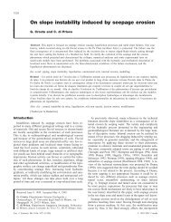
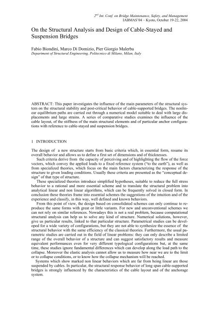
By taking into account the large amount of geometrical, topological and stiffness characteristicswhich influence the actual behavior of the bridge, a systematic structural analysis can becarried out only through non linear numerical methods.A numerical model suitable to deal with large displacements and large strains, typical ofthese system, has been developed. Through the principle of virtual works, developed accordingto the Updated Lagrangian formulation, a truss and a beam element have been introduced.The extension of such a formulation to complex structures gives a central role to the numericaltechniques for solving non linear problems in presence of singular points and of unstable behaviors.As known, the classical Newton-Raphson Method allows us to follow the equilibriumpaths working by load increments, but it is not able to follow post critical behaviors. In order toextend the analysis to the post critical field, the arc length method has been used. The methodhas been improved by specific procedures, able to detect the bifurcation points and the pathswhich depart from these points. This numerical approach has been tested through many benchmarks.In this paper a series of comparative studies examines the influence of the cable layout, ofthe stiffness of the main structural elements and of particular anchoring configurations with referenceto cable stayed and suspension bridges.2 CABLE-STAYED BRIDGESWe refer to the cable stayed bridge geometry shown in Figure 1, having the mechanical andgeometrical characteristics listed in Table 1. In the same table the stay pretensioning is given. Inthe following, the influence of the cable layout on the overall bridge stability is investigated. Tothis aim, we intend to study the cases described in Table 2.PACC40m 21m 21mSEZ.4SEZ.3SEZ.21PP90m 200m 90m2 3 4 5 6 7 8 9 10 11 12 13 14 15 16 17 18 19 20 21 22 23 24(a) Earth AnchoredDeckStay(b) Semi Earth Anchored(c) Self AnchoredFigure 1. Structural model of the cable-stayed bridge.Table 1. Mechanical and cross-sectional properties, and pretensioning of the stays.Element E [GPa] I x [m 4 ] I y [m 4 ] A [m 2 ] w [kN/m]Deck 40 4.0896 236.09 8.0759 100Pylon(0-40m) 40 1.3482 13.843 5.00 –Pylon(40-61m) 40 0.722 2.7750 2.70 –Pylon(61-82m) 40 0.6219 2.6417 2.30 –Stay(1 e 2) 210 – – 0.01 –Stay(3,4,5,6) 210 – – 0.005 –Pretensioning of the staysStay 1≡24 2≡23 3≡22 4≡21 5≡20 6≡19P N0,i [kN] 4340 3480 2522 2219 1840 1590

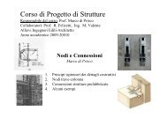
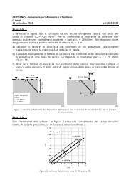
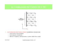
Table 2. Case studied for cable stayed bridges.Model Description(a) Reference case: Fan shaped cable stayed bridge, with earth anchored lateral stays.(b) Model (a) with roller support at right end (semi-earth anchored system).(c) Model (a) with both ends roller supported. The lateral stays are anchored at the deck (selfanchoredsystem).0 Reference case: Fan shaped cable stayed bridge, semi-earth anchored.1-6 The stays, which in Model 0 converge to the top of the antennas, are no longer anchored allin one point but reach the antenna with variable distances within each other.7 Model 0, with stays having such a distance within each other as to reach the harp configuration.(d) Fan shaped cable stayed bridge, with self-anchored lateral stays and deck flexural stiffnessequal to a quarter of that of the starting Model 0.(e) Harp shaped cable stayed bridge, with self-anchored lateral stays and deck flexural stiffnessequal to a quarter of that of the starting Model 0.2.1 Comments on the behavior of (a), (b), (c) Models (Figure 2)The earth anchored Model (a) is stable and behaves like a typical tension hardening system. Theexternal cables (Cable 1 and Cable 24) constrain the heads of the antennas against longitudinaldisplacements and convey the horizontal components of the stay tension directly to the earth.Model (b) presents a limit point (λ = 15.73) caused by the instability of the right antenna,which is now free to move, while Cable 24 loads the deck, contributing to cause large longitudinaland vertical displacements.Model (c) has a limit point (λ = 15.48) which, in this particular case, is a bit higher than forModel (b), but it presents a worse post critical behavior without recovering stiffness after havingreached the limit point.30λ25λ=16.482015λ=15.7310(a) Earth Anchored System5(b) Semi Earth Anchored System(c) Self Anchored SystemV/L0-0,2 -0,18 -0,16 -0,14 -0,12 -0,1 -0,08 -0,06 -0,04 -0,02 0Figure 2. Live-load deflection path of cable-stayed bridges with different typology of supports.2.2 Comments on the behavior of 0 ÷ 7 Models (Figure 3)The sequence of Models 0-7 realizes the gradual development of stay geometry from pure Fanto a pure Harp configuration. For each of these Models, Figure 3 shows the load deflection pathassociated to the vertical displacement at the middle of the central span.For Models 0-3 we have increasing limits points (λ = 15.73, 16.67, 18.24), with a certain tensionhardening post-critical branch and, for Model 1, a hint of snapback.For Models 5-7 there are no limit points and the system appears stiffer than in the previouscases.

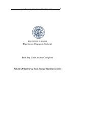
∆=0∆=4m04∆=1m∆=5m15∆=2m∆=6m26∆=3m∆=7m3756730λ252 3 4102015105V/L0-0,2 -0,18 -0,16 -0,14 -0,12 -0,1 -0,08 -0,06 -0,04 -0,02 0Figure 3. Evolution of the live load-displacement path with the variation of the configuration of thesuspension system from the Fan to the Harp arrangement.2.3 Comments on the behavior of (d)-(e) Models (Figures 4 and 5)It must be remembered that the sequence of results shown in Figure 3 is specialized to a particularcombination of dimensions and of stiffness characteristics. From these results, for instance,it appears that there is always a limit point for those systems having the cables converging at thetop of the antennas, while for Harp type systems the behavior appears to be stable and tensionhardening. This can be simply explained by observing that in the Fan case the stay action resultsin a concentrated force acting at the top of the antenna, while in the Harp system the verticalcomponents of the stay action are distributed along a certain height (Figure 4.a).In reality, for usual dimensions and stiffness distributions, is the Harp system the critical one.In fact, in a Fan system the applied load is transferred through the CB stay to the three BOD barsystem and, in this way, to the rigid supports (Figure 4.b). In the Harp system the applied loadacts directly on the CBAD system and it is transferred to the supports involving also the flexuralstiffness of the deck. Moreover in the Harp systems the stays have a lower vertical slope thanfor the Fan and this provokes a higher compression force in the deck. Figure 5 compares theload deflection path for the two cases (d-Fan) and (e-Harp).

FAN SystemHARP SystemB(a)BOACDA(b)DCFigure 4. Role of the suspension system in the structural stability of (a) the pylons and (b) the deck.O16λ14121086λ=5.294FANHARP2V/L0-0,1 -0,09 -0,08 -0,07 -0,06 -0,05 -0,04 -0,03 -0,02 -0,01 0Figure 5. Load deflection path of the Fan and Harp systems with low stiffness of the deck.3 SUSPENSION BRIDGESIn suspension bridges, the forces acting on the main cable, can be transferred to the earth directlythrough anchor blocks at the end of the side spans or can be self-contained by the longitudinalaction of the deck (self-anchored systems). The self-anchored systems do not require thevolumes of the anchor blocks. On the other hand the stiffening girder, heavily compressed, willrequire a larger cross section.3.1 The case of the Great Belt BridgeThe present application refers to the basic dimensions of the Great Belt Bridge, shown in Figure6. The bridge has a central span length s c = 1624 m, two lateral spans lengths s l = 535m, heightof the pylons h = (180+77.6) = 157.6 m, sag of the cable f =180 m. Based on such scheme, acomparative study has been carried out by varying some fundamental characteristics of thebridge. In particular, the cases listed in Table 3 have been examined.

535m1624m535m77,6 m180 mFigure 6. Great Belt Bridge. Structural scheme and basic dimensions.Table 3. Cases studied for suspension bridges.ModelDescription0 Real case: suspension bridge earth anchored (stable).1 The bridge of model 0, but self-anchored. (Area and Inertia of the deck are A=0.5m 2 ,J=1.66m 4 ).2 The bridge of Model 1 with increased deck stiffness (A = 0.9 m 2 , J = 3.32 m 4 ).3 The bridge of Model 1 with increased deck stiffness (A = 1.4 m 2 , J = 4.98 m 4 ).4 The bridge of Model 1 with height pylons increased from 257.6m to 277.6m, but maintainingthe sag of the cable f = 180 m.5 The bridge of Model 4 with increased deck stiffness (A = 0.8 m 2 , J = 4.0 m 4 ).6 Equal to Model 1, but having a truss hanger net.7 Equal to Model 1, but with hangers having a variable slope along the side spans.8 Equal to Model 7 with increased deck stiffness (A = 0.8 m 2 , J = 3.32 m 4 ).The results are shown in Figure 7. The first diagram presents the values of the load multiplierat the limit point in function of the inertia of the deck. The little circles used to mark the limitpoints allow us to recognize if a limit point is stable or if it is followed by unstable branches.The main conclusions of these comparative studies can be synthesized as follows:– Suspended, earth anchored systems are generally stable.– The behavior of suspended, self-anchored systems is sensitive to the action of the deck andto the slackness of the hangers.Furthermore, for suspended, self-anchored systems we can observe that:– There are limit and bifurcation points which lead to post critical and generally unstable response,with snap back effects.– The limit load multiplier can be augmented by stiffening the deck. However, it must be keptin mind that the increase in weight causes an increase in the axial force, with the possibilityof a critical behavior taking place in the pylons and not in the deck.– An increment of the pylon height involves a greater slope of the main cables: this involvethat a greater portion of the total force in the cables is conveyed directly to the earth throughthe bearings, while a lower fraction of this force contributes to the axial component in thedeck. This brings to a higher value of the load multiplier.– The simultaneous increase of the deck inertia and of the pylons height do not produce relevantpositive effects, because the critical behavior depends on the pylons again, while thepiers are higher and more stressed.– It is possible to obtain relevant increments in the limit load multiplier just by increasing theslope of the hangers in the lateral spans, without having any simultaneous increase in costsor in dead loads, as can be seen in models 7 and 8.3.2 The case of the Messina Strait BridgeA final example of application regards the influence of an elastic connection between the maincable and the anchor blocks of the Messina bridge. Figure 8 shows the model of the bridge. Figure9 shows a family of curves, corresponding to different stiffness of the elastic connection,which show how the vertical displacements of the point at the top of the anchorage lever dividedby the lever length (V/H), varies in function of a scalar multiplier λ of the uniform live load appliedto the deck.

λFOR MODEL 0 (REAL CASE EARTH ANCHORED)STABLE AND NEARLY LINEAR BEHAVIOR (λ =∞)15Ratio HPylons/LDeck=1:8λ=13.534I=1.66mA=0.5m 2MODEL 8λ=18.014I=3.32m2A=0.8mMODEL 4MODEL 7λ=12.994I=1.66mA=0.5m 2MODEL 2λ=12.414I=3.32mA=0.9m 2105MODEL 1λ=7.184I=1.66m2A=0.5mMODEL 6λ=7.744I=1.66mA=0.5m 2MODEL 5Ratio HPylons/LDeck=1:8λ=8.514I=4.0mA=0.8m 2MODEL 3λ=8.264I=4.98mStable Limit Point0Instable Limit PointA=1.4m 2 64Deck Stiffness I(m )01 2 3 4 58λ14λ712610Model 15432Model 286412V/L0-0.005 0 0.005 0.01 0.015 0.02v/L0-0.02 -0.01 0 0.01 0.02 0.03 0.04 0.05 0.06 0.07 0.0818λ16λ16141412Model 3121086Model 410864422V/L0-0.035 -0.03 -0.025 -0.02 -0.015 -0.01 -0.005 0 0.005v/L00 0.02 0.04 0.06 0.08 0.1 0.12 0.14 0.16 0.182018λ98λ167Model 514121086Model 665434221v/L0-0.18 -0.16 -0.14 -0.12 -0.1 -0.08 -0.06 -0.04 -0.02 0v/L00 0.02 0.04 0.06 0.08 0.1 0.12 0.14 0.16 0.1814λ20λ1812161014Model 7864Model 812108624v/L00 0.02 0.04 0.06 0.08 0.1 0.12 0.14 0.16 0.182v/L00 0.05 0.1 0.15 0.2 0.25Figure 7. Great Belt Bridge. Live load-displacement paths for the models 1-8 described in Table 3.

20.00m777m 183m3300m183m 627m300m358mHangerMain CableRigidConnectionDeckPylon4.80mPylonMain CableSupportAnchorSystemFigure 8. Structural Model of the Messina Strait Bridge.21V0250λk2001502Rigid ElementK=100x10^3 MN/mK=10x10^3 MN/mK=5x10^3 MN/mK=2.5x10^3 MN/mK=1x10^3 MN/mK=0.75x10^3 MN/mK=0.5x10^3 MN/m100501-0,35 -0,3 -0,25 -0,2 -0,15 -0,1 -0,05 0 0,05 0,1Figure 9. Messina Strait Bridge. Live load-displacement paths with respect to the ratio between the verticaldisplacement V of the point at the top of the anchorage lever and its height H (V/H).0V/H4 CONCLUSIONSThe role played by the main parameters of the structural system in driving the structural stabilityand post-critical behavior of cable-supported bridges has been investigated. In particular, a parametricstudy based on a numerical model suitable to deal with large displacements and largestrains has been carried out. The results of this study allow to highlight and quantify the highsensitivity of the structural response of cable-stayed and suspension bridge with respect to thecharacteristics of both the suspension and anchorage systems.5 REFERENCESBonet J., Wood, R., 1977. Nonlinear continuum mechanics for finite element analysis. Cambridge UniversityPress.Bontempi, F., Malerba, P.G., 1996. The control of the tangent formulation in structural non linear problems,Studies and Researches, 17, Graduate School for Concrete Structures, Politecnico di Milano,Milan, Italy (in Italian).Bontempi, F., Malerba, P.G., 1997. The Role of Softening in the Numerical Nonliner Analysis of ReinforcedConcrete Frames, Structural Engineering and Mechanics, 5(6), 785-801.Crisfield, M.A., 1991. Non-linear finite element analysis of solids and structures, John Wiley & Sons.Di Domizio, M., 2003. Geometrical non linear analysis of cable stayed and suspension structures. Dissertation,Politecnico di Milano, Milan, Italy (in Italian).Gimsing, N., J., 1988. Cable supported bridges, John Wiley & Sons.Riks, E., 1979. An incremental approach to the solution of snapping and buckling problems, InternationalJournal of Solids Structures. 15, 529-551.