CalCOFI Reports, Vol. 27, 1986 - California Cooperative Oceanic ...

REPORTSVOLUMECICTCIBERXXVll1986

CAL I FO R N I ACOOPERATIVEOCEANICFISHERIESINVESTIGATIONSReportsVOLUME XXVllJanuary 1 to December 31, 1985Cooperating Agencies:CALIFORNIA DEPARTMENT OF FISH AND GAMEUNIVERSITY OF CALIFORNIA, SCRIPPS INSTITUTION OF OCEANOGRAPHYNATIONAL OCEANIC AND ATMOSPHERIC ADMINISTRATION, NATIONAL MARINE FISHERIES SERVICE

EDITOR Julie OlfeSPANISH EDITOR Patricia MatraiThis report is not copyrighted, except where otherwise indicated, andmay be reproduced in other publications provided credit is given to theCalifornia Cooperative Oceanic Fisheries Investigations and to theauthor(s). Inquiries concerning this report should be addressed toCalCOFl Coordinator, Scripps Institution of Oceanography, A-027, LaJolla, California 92093.EDITORIAL BOARDlzadore BarrettRichard KlingbeilJoseph ReidPublished October 1986, La Jolla, California

CalCOFI Rep., Vol. XXVII, 1986CONTENTSI. Reports, Review, and PublicationsReport of the CalCOFI Committee .................................................... 5Review of Some California Fisheries for 1985 ........................................... 7The 1985 Spawning Biomass of the Northern Anchovy. Andrew G. Bindman .................. 16The Relative Magnitude of the 1985 Pacific Sardine Spawning Biomass off SouthernCalifornia. Patricia Wolf and Paul E. Smith ...................................... 25Publications ...................................................................... 3211. Symposium of the CalCOFI Conference, 1985SOUTHERN CALIFORNIA NEARSHORE WATERS: SELECTED PATTERNS AND PROCESSES ... 35Physical-Chemical Characteristics and Zooplankton Biomass on the Continental Shelfoff Southern California. James H. Petersen, Andrew E. Jahn, Robert J. Lavenberg,Gerald E. McGowen, and Robert S. Grove ...................................... 36Abundance of Southern California Nearshore Ichthyoplankton: 1978- 1984. Robert J.Lavenberg, Gerald E. McGowen, Andrew E. Jahn, James H. Petersen, and Terry C.Sciarrotta ................................................................. 53Can We Relate Larval Fish Abundance to Recruitment or Population Stability? A PreliminaryAnalysis of Recruitment to a Temperate Rocky Reef. John S. Stephens, Jr., Gary A.Jordan, Pamela A. Morris, Michael M. Singer, and Gerald E. McGowen ............. 65Inshore Soft Substrata Fishes in the Southern California Bight: An Overview. Milton S. Love,John S. Stephens, Jr., Pamela A. Morris, Michael M. Singer, Meenu Sandhu, andTerryC.Sciarrotta .......................................................... 84111. Scientific ContributionsEvaluating Incidental Catches of 0- Age Pacific Hake to Forecast Recruitment. Kevin M.Bailey, Robert C. Francis, and Kenneth F. Mais .................................. 109Peruvian Hake Fisheries from 1971 to 1982. Marco A. Espino and ClaudiaWosnitza-Mendo ............................................................ 113Relative Abundance of Four Species of Sebastes off California and Baja California. John S.MacGregor ................................................................ 121Large Fluctuations in the Sardine Fishery in the Gulf of California: Possible Causes. DanielLluch-Belda, Francisco J. Magallon, and Richard A. Schwartzlose ................. 136Modelo Polinomial para Crecimiento Individual de Larvas de la Anchoveta Norteria,Engraulis mordax. Casimiro Quitionez-Velazquez y Victor Manuel Gomez-Murioz ....... 141Offshore Entrainment of Anchovy Spawning Habitat, Eggs, and Larvae by a Displaced Eddyin 1985.PaulC.Fiedler ..................................................... 144Prey Size Selectivity and Feeding Rate of Larvae of the Northern Anchovy, Engraulis mordaxGirard. Patricia D. Schmitt ................................................... 153Development and Distribution of Larvae and Pelagic Juveniles of Ocean Whitefish,Caulolatilus princeps, in the CalCOFI Survey Region. H. Geoflrey Moser, BarbaraY. Sumida, David A. Ambrose, Elaine M. Sandknop, and Elizabeth G. Stevens ......... 162Distribution of Filter-Feeding Calanoid Copepods in the Eastern Equatorial Pacific. FernandoArcosandAbrahamFleminger ................................................ 170Life Cycle of the Marine Calanoid Copepod Acartia californiensis Trinast Reared underLaboratory Conditions. Antonio Trujillo-Orti'z .................................... 188The Vertical Distribution of Some Pelagic Copepods in the Eastern Tropical Pacific. Ya-QuChen ..................................................................... 205The Temperate and Tropical Planktonic Biotas of the Gulf of California. Edward Brinton,Abraham Fleminger, and Douglas Siegel-Causey ................................. 228Frame Trawl for Sampling Pelagic Juvenile Fish. Richard D. Methot .................. 267Instructions to Authors ................................................................ 279CalCOFI Basic Station Plan ................................................. inside back cover

COMMITTEE REPORTCalCOFI Rep., Vol. XXVII, 1986Part IREPORTS, REVIEW, AND PUBLICATIONSREPORT OF THE CALCOFI COMMllTEEThe member agencies of CalCOFI remain stronglycommitted to cooperative partnership as a means ofmaking optimal use of public resources, sharing ideasin research, and providing a public forum to examineand discuss fisheries problems that concern the peopleof California. The pelagic ecosystem off the coast ofthe Californias is multidimensional, dynamic, andcomplex, and research on that system requires opennessto new ideas and approaches, with assurance ofthe continuity of fundamental CalCOFI data bases. Asa result, CalCOFI scientists’ work follows two majortrajectories. First, quarterly cruises are made off thecoast of California to measure the same physical,chemical, biological, and meteorological variablesyear after year. On these cruises, new technologies, includingsatellite-mediated information gathering, areemployed. Second, this information is used to form hypothesesand test them ashore and at sea, using stateof-the-artmethods such as satellite-tracked drogues,very high-frequency sonar, automated samplingdevices, and satellite imaging.The 36-year time series of physical, chemical, biological,and meteorological data from the CaliforniaCurrent, collected and processed by the CalCOFIteam, constitutes an enormous challenge in data-basemanagement and data access. The Southwest FisheriesCenter has continued to develop a user-friendly systemfor access to the entire data suite. In addition to the developmentof software, the process has required theverification of some earlier larval identifications in thelight of later knowledge. The system, when completed,will make a large body of data readily accessible toqualified researchers, and will greatly increase theknowledge available from CalCOFI’s extensivecollections.Determining the spawning biomass of sardines,when their biomass is very low, has been a problem inthe past. During the last year, Patricia Wolf of the CaliforniaDepartment of Fish and Game, and Paul Smithof the National Marine Fisheries Service (NMFS) usedthe newly developed egg production method to make acost-efficient, quantitative determination of the relativemagnitude of sardine spawning biomass duringtimes of low biomass levels. This method was employedduring May 1985 to determine that the spawningbiomass was at least 20,000 short tons, permittingthe opening of a 1,000 ton sardine fishery on January 1,1986. The 1986 sardine fishery is the first since themoratorium took effect in 1974.CalCOFI was organized in 1949 as a response to theneeds of California’s fishing industry, and has a longstandingrelationship of cooperation with and serviceto the industry and to governmental managers. In1985, CalCOFI researchers from the Southwest FisheriesCenter and from the California Department of Fishand Game consulted with industry scientists to discussmanagement options for Pacific mackerel. Theirrecommendations resulted in the adoption, by the statelegislature, of new law for managing this stock.The CalCOFI Committee sponsors a conferenceeach October to discuss the status of knowledge aboutfisheries; the biology of fishes; their environment, includingphysics, chemistry, meteorology, and-fromtime to time-fishing gear; and the industry and itspolitics. The 1985 conference at Idyllwild, California,included a symposium convened by John Grant of theCalifornia Department of Fish and Game, entitled“Southern California Nearshore Waters: SelectedPatterns and Processes.” Some of the papers presentedat that symposium are included in this volume.During the past year, CalCOFI personnel ofNMFS’s Southwest Fisheries Center, the Marine LifeResearch Group at Scripps Institution of Oceanography,and the California Department of Fish and Gamehave fielded four CalCOFI survey cruises of 15 days’duration, two trawl survey cruises, one biomass cruise,two Sardine-Anchovy Program cruises, and one Doversole trawl-survey cruise. The CalCOFI Committeewishes to acknowledge the officers and crews ofNOAA research vessels David Starr Jordan andMcArthur and the University of California’s R/V NewHorizon for their support. The data have been reportedin the Scripps Institution of Oceanography ReferenceSeries, the CalCOFI Data Report Series, and other datareports and documents.The Committee wishes to thank Herbert Frey of theCalifornia Department of Fish and Game for his manyyears of service to the CalCOFI Committee. Herb hasserved as alternate to the Committee, as a member fortwo terms, and as CalCOFI Coordinator. He has alsoserved as editor of CalCOFI Reports and as executivesecretary of the Marine Research Committee of5

FISHERIES REVIEW: 1985CalCOFl Rep., Vol. XXVII, 1986REVIEW OF SOME CALIFORNIA FISHERIES FOR 1985California Department of Fish and GameMarine Resources Region245 West BroadwayLong Beach, California 90802Total 1985 landings of fishes, crustaceans, and mollusksdeclined for the fifth straight year. Landings declined21 % from 1984 to a level 52% below the averagefor the last ten years. Continuing closures of Californiatuna processing plants were the primary reason for thepersistent decline.Landings of pelagic wetfishes increased slightly forthe first time in four years (Table 1). Both the Pacificherring and market squid fisheries rebounded from thelow levels recorded during the recent warm-water period.While mackerel landings remained relativelystable, and the anchovy reduction fishery faded, thePacific sardine resource continued a modest trend ofapparent increased abundance.Groundfish landings increased somewhat over 1984levels, with significant gains for flatfishes and Pacificwhiting almost offset by declines for rockfishes.Swordfish landings set a new high; for the first time inseveral years harpoon vessels contributed considerably,augmenting the catches of the drift gill net fleet.Pacific ocean shrimp landings increased for the secondstraight year.Moderate decreases were recorded for the Dungenesscrab and lobster fisheries, while albacore decreasedby almost 50% from 1984 landings.Sportfish landings were more comparable to thoseyears with “normal” water temperatures: there werefewer exotics, and salmon were healthier.PACIFIC SARDINEThe moratorium on commercial fishing for Pacificsardines (Surdinops sagux cueruleus) remained in effectduring 1985 because the spawning biomass wasassessed as remaining below the 20,000 tons requiredbefore a fishery may be allowed. However, recent occurrencesof sardines in mackerel and live bait catches,in California Department of Fish and Game (CDFG)sea surveys, and in CalCOFI ichthyoplankton surveys,as well as observations by aerial fish spotters indicatedthat the biomass might be approaching 20,000tons. CDFG and the National Marine Fisheries Service,Southwest Fisheries Center designed and conducteda survey in May to determine whether thesardine spawning biomass had exceeded this level. TheTABLE 1Landings of Pelagic Wet Fishes in California in Short TonsYear19641965196619671968196919701971197219731974197519761977197819791980I98 I1982198319841985”Pacificsardine6,56996243974625322 114918676732765183831145388259652Northernanchovv2,4882,86631,14034,80515,53867,63996,24344,85369,101132,63682,691158.510I24,9 I91 11,47712,60753,88147,33957,65946,3644,7403,2581,792Pacificmackerel13,4143,5252.3155831,5671,17931 I785428671443285,97512,54030,47 I32,64542,9133 1 -27535,88246,53 I38,100Jackmackerel44,84633,33320.43 119,09027,83426,96123,87329,94125,55910,30812,72918,39022,27450,16334,45618,30022,42815,67329,l IO20,27211,76810,316Pacificherring175258121I36I7985158120631,4102,6301,2172,4105,8274,9304,6938,8866,571I 1,3228,8294,2418,801Marketsquid8,2179,3109,5129,80112,46610,39012,29515,75610,3036,03 I14,45211,81110,15314,12218,89922,02616,95825,91517,9512,01062210,881Total75,70950,25463,95864,48957,646106.307133,10190,897105,266150,489112,576190,075l60,l I1187,57083,437129,389128.294148,762136,16772,12166,67970.542”Preliminary7

FISHERIES REVIEW: 1985CalCOFl Rep., Vol. XXVII. 1986survey used the presence of sardine eggs to assess theextent of spawning area in southern California waters.Sardine spawning covered an estimated 670 n.mi.2,which was determined to be characteristic of a biomassof at least 20,000 tons. As provided by current law,CDFG announced the opening of a 1,000-ton fishery tobegin January 1, 1986. Apart from the 75-ton live baitquota initiated last year, this is the first directed take ofsardines allowed in California since the moratoriumtook effect in 1974.The trend of increasing occurrences of sardines inthe mackerel fishery, which slowed last year, appearsto have resumed. An estimated 652 tons of sardineswere landed incidentally with mackerel during 1985(Table 1). This is the largest annual take in 20 years.Monterey landings accounted for 6% of the incidentalcatch, and local fishermen reported sighting largeschools of sardines in Monterey Bay on several occasions.The proportion of observed mackerel landingscontaining sardines increased from 30% in 1983and 1984 to over 57% during 1985. Sardines constituted1.3% of the overall 1985 “mackerel” catch;during March-April sardines were nearly 3% of thecatch. Length frequencies of incidentally caught sardinesshow an increasingly broader distribution from1983 through 1985, indicating that recruitment hascontinued.Sardine landings in live bait declined to .roughly25% of the 1984 estimated landings, and failed to reachthe 75-ton annual quota. This probably resulted from adecreased demand for sardines rather than a decline inavailability. Live bait fishermen often targeted insteadon squid, which were available for the first time in recentyears and are often preferred as bait for certain biggame fish. Legislation passed in 1985 increases the annuallive bait quota for sardines from 75 to 150 tons, effectiveJanuary 1, 1986.During CDFG experimental young fish surveys inJuly and August, only adult sardines were captured.Evidence of sardine recruitment was not observed untilSeptember, when young-of-the-year fish appeared inboth the live bait catch and sea survey trawls. Adultand juvenile catch frequencies during the Septembercruise were lower than last year’s; however, the catchfrequency of juveniles suggests that the 1985 year classis similar in strength to the 1984 year class and considerablyweaker than the 1983 year class. Adult fishcaptured during the sea survey cruises were in progressivelymore advanced stages of prespawning conditionfrom July through September. Also, a greaterproportion of adult sardines occurring in the mackerelfishery were nearing spawning in the late summer thanin the spring. These observations suggest that a largeportion of spawning occurred during late summer andearly fall this year; the historical sardine populationspawned mostly in spring.Current state law provides for the rehabilitation ofthe sardine resource. During the process of rehabilitationa small fishery is allowed. If the spawning populationincreases beyond 20,000 tons, CDFG mayincrease the seasonal quota, but at such a rate as toallow for the continued recovery of the population.Only limited markets exist now for sardines, and it remainsto be seen whether new markets and uses will developas the resource recovel-s.NORTHERN ANCHOVYAt least one processor in both the northern (north ofPoint Buchon) and southern permit areas issued ordersfor northern anchovy (Engradis rnordax) for reductionduring the 1984-85 season. Fishermen, however,found anchovies unprofitable and concentrated theirefforts on mackerel. The anchovy price per tondropped from $38 to between $25 and $30, and fishermenreported that large anchovy schools were not locallyavailable in either permit area.A single landing of 77 tons was made during the1984-85 reduction season (Table 2). This landing occurredat Terminal Island in November 1984, againstthe southern area quota of 6,250 tons. No landings forreduction purposes were made toward the northernarea 1984-85 season quota of 694 tons.Using an egg production biomass assessmentmethod, the National Marine Fisheries Service esti-TABLE 2Anchovy Landings for Reduction Seasons in theSouthern and Northern Areas, in Short TonsSouthern NorthernSeason area area Total1966-671967-681968-691969-701970-711971 -721972-731973-741974-751975-761976-771977-781978-791979-801980-811981-821982-831983-841984-85**Preliminary29,58985225,3148 1,45380,09552,05273, I67109,207109,918135,619101,43468,47652,69633,38362,16145,1494,92570778,0215,6512,7362,0206571,3742,35211,3806,6695,2915,0077,2121,1742,3654,7364,9531,2701,765037,6106,50328,05083,47380,75253,42675,519120,587116,587140,910106,44175,68853,87035,74866,89750, 1026,1951,835778

FISHERIES REVIEW: 1985CalCOFI Rep., Vol. XXVII, 1986mated the 1985 northern anchovy spawning biomass at574,421 tons (521,000 metric tons). The U.S. optimumyield for the 1985-86 season was set at 159,750tons, and the harvest quota for reduction purposes wasset at 154,350 tons. Allocations established were10,000 tons for the northern permit area, and 144,350tons for the southern area.The 1985-86 reduction season opened on August 1in the north and September 15 in the south. Approximately909 tons of anchovy were landed between November15 and December 30, 1985. All landings weremade in the northern permit area by two boats fishingjust outside the Monterey Bay breakwater. Efforts tofill reduction orders dropped off as fish moved out ofthe area.Statewide reduction landings of northern anchovyfor 1985 were 909 tons. Nonreduction landings totaled883 tons. The live bait catch was estimated at 5,055tons. Bait was highly available year-round.Trawl surveys during 1985 indicate dominance bythe 1984 and 1983 year classes (66% and 22% bynumber, respectively, in survey samples). Althoughyoung-of-the-year ( 1985 year-class) fish made a strongshowing in live bait hauls from June through December,reports of poor catches of young fish in the 1985Mexican reduction fishery, and their poor representationin CDFG recruitment surveys indicate that the1985 year class may actually be weak.JACK MACKERELApproximately 10,320 tons of jack mackerel(Truchurus symmetricus) were landed during 1985.Jack mackerel constituted roughly 21 % of total mackerellandings. This marks the seventh consecutive yearthat jack mackerel have contributed less than Pacificmackerel to the California mackerel fishery. It is thesecond consecutive year that jack mackerel have contributedsuch a low proportion of the mackerel fisherysince this species first supported a fishery in the late1940s.Jack mackerel dominated landings only during January,when landings of Pacific mackerel were limited byinterseason restrictions, and overall mackerel landingswere the lowest of the year. Jack mackerel were mostlyunavailable or not sought after in southern Californiaduring the last four months of the year. The compositionof northern California catches varied greatlythroughout the year, with jack mackerel constitutingless than 1 % of the catch in October and more than 95%of the catch in January and February. Calculatedthroughout the year, jack mackerel made up 23% of thenorthern California mackerel catch and 20% of thesouthern California catch. This is in contrast to 1984and 1983, when jack mackerel contributed a consider-ably larger proportion of the mackerel landings in thenorth than in the south.Sea surveys conducted during 1985 indicate fair togood recruitment for the 1985 year class of jackmackerel.PACIFIC MACKERELThe 1984-85 season (July I-June 30) for Pacificmackerel (Scomber juponicus) was closed on December20 because the adjusted season quota of 26,000tons has been landed. Interseason restrictions were ineffect through January, limiting the take of Pacificmackerel to 50% or less by number, or pure loads of 3tons or less. The season reopened on February 5 afterthe California Fish and Game Commission (FGC), asrecommended by CDFG, augmented the quota with5,000 tons per month for February, March, and April,with uncaught portions of the monthly allotments to beadded to the next month’s quota. The quota increase resultedfrom a reevaluation of the 1984-85 Pacificmackerel total biomass, finally estimated to range between131,000 and 242,000 tons. For the first time thisestimate included consideration of Mexican commercialand U.S. recreational catches in cohort analysis.Landings continued to be low despite quota increases,because southern California processors imposeda landing limit of approximately 70 tons per boatper month through March. In April the landing limitwas increased to 50-60 tons per boat per week, but theprice per ton was lowered from $190 to $163. On April24, the FGC added another 15,000 tons to the season’sallowable catch, bringing the 1984-85 season quota to56,000 tons. Fishing for the remainder of the seasonwas slow. Although the price was increased to $170 perton, landing limits were decreased to 25 and 50 tons perboat per week, because inventories of frozen mackerelreportedly exceeded last year’s by 60%. In Montereyonly about 1,600 tons of mackerel were landed fromJanuary through June, because fishermen concentratedtheir efforts on squid. The National Marine FisheriesService (NMFS) began to investigate the use of Pacificmackerel in a federal surplus commodities program tohelp ease poor local market conditions, which werepartly caused by competition from foreign countries.The 1984-85 season ended with a total catch of43,270 tons of Pacific mackerel. Approximately 83%was landed in southern California. Pacific mackerelconstituted an average 93% of total mackerel landingsfrom January through June 1985, and 81% of totallandings for the 1984-85 season. Areas where fish werecaught from February through June ranged from off theSanta Barbara coast to outside Santa Monica Bay, andout to Santa Cruz, Anacapa, and Santa Catalinaislands.9

FISHERIES REVIEW: 1985CalCOFI Rep., Vol. XXVII, 1986The 1985-86 season opened July 1, 1985. The Pacificmackerel biomass was estimated to range between178,000 and 260,000 tons, providing a season fisheryquota of 40,000 tons. The season started off slowly,because Terminal Island processors were 'closed formuch of July. Southern California purse seiners fishedup the coast to Morro Bay in August, when landings increasedsubstantially.On September 9, urgency legislation (AB 1197) waspassed. This law (1) requires CDFG, by February 1 ofeach year, to estimate the total Pacific mackerel populationsize for the current season, and the expected sizeat the beginning of the next season; (2) sets the quota at30% (up from 20%) of the population above 20,000tons when the total biomass is between 20,000 and150,000 tons; (3) allows for no quota restrictions (openfishery) when the biomass is greater than 150,000 tons;(4) allows CDFG to adjust quotas during any portion ofthe season; (5) increases the pure-ton interseason restrictionsfrom 3 to 6 tons; and (6) eliminates the 10-inch size limit. Quota restrictions for the remainder ofthe 1985-86 season were subsequently lifted upon considerationof the estimated biomass range.Landings were high in September, but declined inOctober during a dispute over landing limits andprices. Fishing resumed in November, with landinglimits remaining in place and the price reduced to $155per ton. Landings were limited by a lack of orders, particularlyin northern California. December landingswere high, for fish were locally abundant, and ordersincreased.By the end of December approximately 22,870 tonsof Pacific mackerel had been landed for the 1985-86season. Landings for 1985 reached 38,100 tons, ofwhich only 7% was landed in northern California. Thisis a decrease from the 18% northern California contributedto mackerel landings last year. As in 1984, the1980 and 1981 year classes of Pacific mackerel accountedfor the majority of landings. Fish 3 years ofage and younger showed better recruitment than in1984, but the 1982 and 1983 year classes still appearvery weak. The strong showing of the 1984 year class,as 1-year-olds, is encouraging. Young-of-the-year fishdid not enter the fishery during 1985, and sea surveyexperimental cruises to assess recruitment of Pacificmackerel off southern California gave preliminary indicationsthat the 1985 year class may be weak.MARKET SQUIDThe California market squid (Loligo upalescens)fishery landed 10,881 tons during 1985, a very large increaseover the last two years' landings (Table 1).However, this was still 23% below the last ten-yearaverage. The California squid fishery is best describedas two separate fisheries: the northern California (orMonterey) fishery, and the southern California fishery.In Monterey the fishery normally follows a summerfallseason, but has been atypical the last three years.This year the fishery started earlier than normal. Largesquid (seven to eight per pound) were caught in April,although there were signs that they were not abundant.In good years the boats are usually at the dock unloadingtheir catch shortly after sunrise. This year, boatsspent more time looking for squid and arrived at thedock as late as noon, with highly variable fishing success.The initial price was $600 per ton.Fishermen voluntarily increased the spawning escapementby giving the squid two weeks to spawnundisturbed in May. Squid landed during May werestill large, but many were spent, and the overall qualitywas poorer than two weeks earlier. The price droppedto $400 per ton.During the summer, fishing moved northerly, awayfrom the traditional grounds near Monterey to the areabetween Afio Nuevo and Pigeon points. Fishing rangedfrom excellent to spotty, with landings through mid-September. Despite continued effort, commercialboats were unable to catch squid after that time. Partyboats,however, were still successfully jigging squidfor bait in November.For the Monterey fishery, squid were scarcethroughout the year. Although demand was strong,only 4,286 tons were landed. This is a great improvementover the past two years, but is still only 30% ofthe 14,000 tons landed in 1981, the best single year inthe past 40 years.The southern California squid fishery typically has afall-winter season, running from early Novemberthrough February. This pattern had not been followedsince 1982, because of a lack of squid, which was probablyrelated to El Nifio. This year, however, the patternresumed; significant landings began in October andcontinued through the winter. Early in the year, squidwere very large, averaging about 5 per pound; later inthe year, they ranged from 8- 11 per pound.Southern California landings totaled 6,595 tons,75% of which were landed during the last quarter of theyear. The price at the beginning of the year, when squidwas still in very strong demand, went as high as $700per ton. The price then dropped steadily until the end ofthe year, stabilizing at $200 per ton.PACIFIC HERRINGThe Pacific herring (Clupea harengus pallasi) fisheryrecovered in 1985 from the transitory effects of the1982-84 El Nifio. The 1984-85 seasonal (December-March) catch of 8,264 tons exceeded the 7,590-tonstatewide quota and nearly tripled the 1983-84 seasonal10

FISHERIES REVIEW: 1985CalCOFI Rep., Vol. XXVII, 1986catch of 3,000 tons. Annual catch figures for 1985 alsoimproved, more than doubling the 1984 catch (Table1). There was a corresponding economic improvementin the fishery. The base price for 10% roe recovery increasedto $1,000 per ton and resulted in an ex-vesselvalue for the 1984-85 fishery of over $9 million.Population estimates from 1984-85 spawninggroundsurveys in Tomales and San Francisco baysparalleled the improvement in the fishery. After thepoor 1983-84 season, almost 6,600 tons of herring returnedto Tomales Bay this past season, and in SanFrancisco Bay the population increased 15%, to46,000 tons.Herring exhibited good growth characteristics during1984; weight lost during the period of poor growthcaused by El Nifio was regained. The generally goodcondition of herring this year contributed to the successof the 1984-85 fishery.Based on the 1984-85 population estimates, thestatewide herring quota for 1985-86 was increased to8,690 tons. Early 1985-86 season catches have beenexcellent. This, coupled with an increase in the exvesselprice for 10% roe recovery to $1,200 per ton,should result in another very good herring season.GROUNDFISHCalifornia’s 1985 commercial groundfish landings(Table 3), including California halibut (Paralichthyscalijornicus), were 43,730 metric tons (MT) with anex-vessel value of $28 million. This represents an increaseof 2,658 MT or 6% from the previous year, butis still 18% less than the record 1982 catch of 52,152MT. California landings constituted 38% of the total1985 Washington-Oregon-California (WOC) commercialgroundfish harvest. Trawl vessels continued theirhistorical domination of the fishery, landing 81% ofCalifornia’s 1985 commercial catch.Trawl landings of the principal groundfish species,with the exception of lingcod (Ophiodon elongatus)and Pacific ocean perch (Sebastes alutus), increasedfrom 4% to 41% over 1984 levels. Dover sole (Microstomuspacificus), sablefish (Anoplopoma fimbria),and Pacific whiting (Merluccius productus)-speciesof particular sensitivity to market fluctuationsregisteredincreases due in part to robust marketdemand and, in the case of Dover sole, to the continuedexpansion of the Morro Bay flatfish fishery. Trawlcaughtrockfish (Sebastes spp.) landings remainedrelatively stable. The setnet fishery for rockfish andlingcod continued its expansion.Federal and state management regulations for theWOC area restricted the harvest of sablefish, widowrockfish (S. entomelas), and other rockfishes duringthe year. The coastwide widow rockfish optimum yieldTABLE 3California Groundfish Landings (Metric Tons)SpeciesDover soleEnglish solePetrale soleRex soleThorn yheadsWidow rockfishOther rockfishLingcodSablefishPacific whitingOther groundfish19849,7749525905682,1242,78114,7279504,8232,3351,4481985”12,1591,0738639062,9753,06511,8126965, I673,0231.991Percentchange24%13%46%60%40%IO%- 20%- 27%7%29%38%TOTAL 41.072 43,730 6%*Preliminary(OY) was set at 9,300 MT, and the sablefish OY wasset at 13,600 MT. Vessel trip and frequency limits werethe regulatory measures used to provide a year-roundfishery without exceeding harvest quotas or guidelines.The year began with a coastwide widow rockfishtrip limit of 30,000 pounds once per week, but with theoption to land 60,000 pounds biweekly. For the thirdconsecutive year, a 40,000-pound trip limit without afrequency restriction was retained for the rockfishcomplex for the waters from Cape Blanco, Oregon, tothe Mexican border. Unrestricted landings of sablefishwere allowed, with the provision that landings of fishless than 22 inches total length could not exceed 5,000pounds per trip in all areas north of Point Conception.The rapid pace of the WOC fishery necessitated inseasonregulatory measures. On April 28 the biweeklywidow rockfish trip limit was rescinded to reduce therate of landings. This proved to be insufficient, and onJuly 21 the widow rockfish trip limit was reduced to3,000 pounds per trip without a frequency limitation.The latter measure sustained the fishery throughout theyear. It became necessary to impose a sablefish triplimit of 13% of a trawl vessel’s total weight of fishlanded per trip, effective November 25, by which time90% of the OY had been harvested. Sablefish harvestsby other gear types were unaffected. This limit remainedin effect until December 5, when the sablefishOY of 13,600 MT was captured, and landings wereprohibited.DUNGENESS CRABCalifornia Dungeness crab (Cancer magister) landingsduring the 1984-85 commercial season totaled4.75. million pounds. This was 0.58 million poundsless than the previous season.In northern California, fishing began on December4, after a price settlement of $1.25 per pound. The

FISHERIES REVIEW: 1985CalCOFl Rep., Vol. XXVll, 1986price was increased shortly thereafter to $1.75 perpound. Weather during the season was generally good,and 347 vessels trapped 92% of the season’s catchby the end of January. As in the 1983-84 season, fewsublegal crabs were observed. The season closed onJuly 15.Landings for Crescent City, Trinidad, Eureka, andFort Bragg were 2.29, 0.33, 1.38, and 0.17 millionpounds, respectively.A high opening price of $2.00 per pound and lowvolume catches greeted San Francisco crabbers onopening day, November 12. Many fishermen stoppedfishing in December because of low production. Theseason closed on June 30 with a total catch of 0.58 millionpounds. It was a disappointing season after theprevious season’s landings of 0.86 million pounds.PACIFIC OCEAN SHRIMPStatewide landings of ocean shrimp (Pandalus jorduni)in 1985 totaled 3.3 million pounds, increasingfor the second straight year. Areas of production wereArea A (False Cape to the Oregon border) and Area C(Pigeon Point to the Mexican Border). The ex-vesselprice of $0.35 per pound was uniform statewide.Area C landings of 39,000 pounds resulted from acombination of targeted trips for ocean shrimp and incidentalcatches in fisheries for spot and ridgebackprawns. The Area C total represents the lowest annualcatch since 1979. The low price and a scarcity ofshrimp discouraged all but one vessel (double-rigged)from fishing. Inexpensive shrimp imports and improvedcatches in other areas also contributed to thelow effort for ocean shrimp in the Morro Bay and Avilaareas.Landings from Area A (California-Oregon border toFalse Cape) totaled 2.9 million pounds, more thandouble the 1.1 million pounds landed during 1984 butstill well below the 1973-82 average of 4.6 millionpounds. Shrimpers landed an additional 0.45 millionpounds in Area A; these were caught in Oregon waters.The $0.35 per pound price received throughout the seasonwas the lowest ex-vessel price since 1979.Only 31 boats (16 single-rigged and 15 doublerigged)delivered shrimp to Area A ports during theseason (April 1 through October 31); this was the lowestnumber of boats since 1977 (excluding 1983).Single-rigged vessels had an average seasonal catchrate of 398 pounds per hour; double-rigged vesselsaveraged 573 pounds per hour.One-year-old shrimp constituted 87.1 % of allshrimp sampled. The incoming year class (1985) madeup only 2.4% of the samples, but during October theyconstituted 13.9% of the samples. This indicates goodrecruitment. Average counts per pound ranged from152.8 in May to 105.3 in October and averaged 123.6for the season.PELAGIC SHARK AND SWORDFISHDuring 1985, 245 permits were issued for harpooningswordfish (Xiphias gladius), and 227 drift gill netpermits were issued for taking pelagic sharks andswordfish. In addition, 33 permits were issued in a specialcategory authorizing swordfish to be taken by driftgill nets north of Point Arguello.Harpoon fishermen enjoyed their most successfulseason since the record year of 1978, landing approximately0.5 million pounds of swordfish. During 1978an unprecedented 3.8 million pounds were landed. Itis still not clear why record numbers of swordfishmoved into waters off southern California in 1978,since nothing even close to this has occurred before orsince. The success achieved in 1985, however, may beattributable to the use of spotter aircraft. An eight-yearban on the use of spotter aircraft was lifted by the CaliforniaFish and Game Commission late in 1984.Reported swordfish landings by drift gillnetters fellslightly in 1985. Logbook submittals indicated 23,129fish caught for the 1985-86 season (May through January),as opposed to 25,367 fish reported for the sameperiod during the 1984-85 season. A reduction in fishingeffort during the month of January, due mainly toinclement weather, probably accounts for the decreasein total reported landings this past season. Waters adjacentto the escarpment bordering the Southern CaliforniaBight, and the seamounts-particularly Rodriguezand San Juan-remained the most productive fishinggrounds during the 1985-86 season.Preliminary 1985 landings of swordfish will onceagain set a new high mark. Because of the combinedsuccess of harpooners and gillnetters, 5.25 millionpounds of swordfish were reported, with an ex-vesselvalue of $13.4 million.Common thresher shark (Alopias vulpinus) landingsamounted to 1.5 million pounds, equaling the previousseason’s mark. The mean length of fish taken in thisfishery continued to decline in 1985. The 1986-87 seasonwill be shortened by a 2.5-month closure (June l -August 14) in an attempt to take the pressure off what isbelieved to be a depressed thresher shark stock.CALIFORNIA SPINY LOBSTERDaily log returns from the 1984-85 (first Wednesdayin October to first Wednesday after March 15) commercialCalifornia spiny lobster (Panulirus interruptus)fishery documented a precipitous decline in legal lobstercatch. The level was the lowest in 12 years.A spirited anticipation pervaded the fishery; the 440authorized fishermen represented the largest partici-12

FISHERIES REVIEW: 1985CalCOFl Rep., Vol. XXVII. 1986pation in the 15 years since an application fee wasinitiated. But enthusiasm dwindled, and the 474,000trap-hauls from 200 boats made up the lowest reportedeffort since the 1980-81 season, 12% below the peakestablished during the 1983-84 season.Log entries tallied a total sublegal (“short”) retentionof 419,000 animals at a 0.89 catch-per-trap (CPT) rate.Sublegal CPT levels have steadily increased duringthe nine years since sublegal escape ports were firstrequired.A total of 245,000 legal-sized lobsters was logged.Commercial fishery landing receipts documented atotal weight of 400,000 pounds, and an average exvesselprice of $4.00 per pound. Thus the 1984-85 fisherywas valued at $1.6 million, 16% below the previousseason’s estimate. The 0.52 legal CPT rate tied 1973-74 as the poorest season, and catch rates for the monthsof November (0.42 legals) and December (0.39 legals)were the poorest ever in the 12-year history of logbookrecords.Catch success, as measured by pounds-per-hundredtrapping-hours(PPHTH) averaged 1.4, compared to1.7 the previous season. Monthly catch success washighest in October (2.0), declined to 0.9 in December,and recovered modestly to 1.3 in February and March.Depressed catch success was largely restricted tosouthern California’s mainland coast. The lightlytrapped northern mainland (8% of the state’s trappingeffort from Malibu Point to Point Arguello) took 8% ofthe state catch and averaged just under 1.0 PPHTH.South of Santa Monica Bay a concentrated 64% of thetrapping effort took 47% of the state catch at a successrate of 1.1 PPHTH.The Channel Islands portion of the fishery was leastaffected during this off season. Indeed, the effort hereincreased slightly from the previous season. Twentysevenpercent of the state’s trapping effort captured44% of the catch at a success rate double that of themainland.Although the 1984-85 season was disappointing to alarge sector of the fishery-specifically those concentratingtheir efforts along the mainland coast-the outlookis not all bad. A continuation of the high sublegalretention should initiate a rapid recovery of legal recruitmentfrom a presumably recovering standingstock of late juveniles/young adults. Preliminary logreturns indicate that catch success for the 1985-86 seasonhas improved, especially along the northern mainlandcoast.The highly productive but densely trapped southernmainland coast continues to foster unrest among veteranlobster fishermen. Although logbook records indicatethe most strongly recovering sublegal stocklevels in the state, saturation trapping of the nearshorewaters off populous San Diego, Orange, and LosAngeles counties effectively limits most fishermen’seconomic gain to the high catchability months ofOctober and November. High competition for the earlyseason profits has created a spiraling escalation of trapdeployment. Overcapitalized fishermen can incur disastrouslosses from sudden storms, poaching, theft, orconcurrent boating activity. Turnover among participantsis high.Stock conservation management seems to be perpetuatingbiologically sound harvest rates, and gradualincrease is expected in the near future. However, socioeconomicconsiderations may shift the fishery tolimited-entry management. Preliminary legislation hasbeen initiated by San Diego-based veteran fishermenand processors in this regard.ALBACOREThe 1985 albacore (Thunnus alafunga) season had afairly traditional start, with an excellent bite near MidwayIsland at the end of May, and fish appearing offsouthern and Baja California in June. By the end ofJune, fish had been spotted as far north as MendocinoRidge (about 150 miles west of Cape Mendocino).During the last half of July, commercial boats werefishing from northern Baja California to the Oregon-Washington border. By the end of August, the bestalbacore fishing was along the Mendocino Ridge.Much of September’s fishing was hampered by roughweather, but most vessels concentrated their efforts offPoint Arena and Bodega Bay when weather permitted.During early and mid-October, many boats were workingtheir last trip of the season.The 1985 season total for California was about 7,200tons. Approximately 1.5% of this was accounted for byfishermen retailing their catch directly to the public.The season total was a little more than half the previousseason’s landings. The 1985 landings also fell 17% belowthe last 10-year average and 36% below the last 25-year average (1 1,182 tons). During 1984 the southernCalifornia purse seine fleet contributed significantly tothe catch. This year, as is more typical, the fish werenot readily available and schooling at the surface, andso were not vulnerable to round haul nets.As in the recent past, there were very low landings inOregon and Washington this season. Approximately750 tons were landed in Oregon and 150 tons in Washington.This brought the WOC fishery landings toabout 8,100 tons, or 60% of the last ten-year coastwideaverage. California has historically landed about 60%of the albacore caught in the WOC fishery, but over thelast few years this percentage has shifted. Last yearCalifornia contributed 93% of the total tonnage, andthis year about 85%. To help put this in perspective on13

FISHERIES REVIEW: 1985CalCOFl Rep., Vol. XXVII, 1986an ocean-wide scale, the WOC fishery lands roughly10%-20% of the annual Pacific-wide catch.A 1985 price agreement of $1,300 per ton for fishweighing 9 pounds or more, and $950 per ton for fishless than 9 pounds was reached in June between PanPacific Cannery and the Western Fishboat OwnersAssociation. During the summer the price droppedtwice, bringing the rate down to $1,000 per ton for fishsold directly to the cannery. This price was as low asthe rates in the mid-1970s. Shipping charges continuedto be deducted from albacore sales at other locations.In 1984, the prices opened at $1,400 per ton for fish 9pounds or more and $1,125 per ton for fish less than 9pounds. By the end of the season, prices had declinedto $1,150 per ton and $875 per ton.Market demand has been one of the most significantinfluences on the fishery. Pan Pacific at TerminalIsland was the only cannery to process and can albacorethis season. The other major cannery, Starkist,stopped processing tuna in the United States in October1984. This year it did continue, however, to purchasealbacore, shipping it to Puerto Rico for processing.Fewer buyers and low prices, combined with occasionalwholesaler buying limits, discouraged manyfishermen. Considering that southern California sportboats reported fair to excellent fishing this season, thelow commercial landings are probably due more to reducedfishing effort than fish availability.In the fall of 1983, U.S. and Japanese scientists metto discuss the status of the Pacific-wide population.They concluded that the stock appears to be well exploited,and is being fished near the estimated ranges ofmaximum sustainable yield.R EC R EAT1 0 N AL F I S H E RYThe catch record of sport anglers fishing on commercialpassenger fishing vessels (CPFVs or partyboats)roughly reflects the success of ocean-goinganglers on private boats. These two groups account forthe vast majority of the marine sportfish catch. Duringthe past four years, this catch record has demonstratedwide fluctuations in relative catch success for manyspecies as a result of the 1982-84 El Nifio phenomenon.Even though the onset of El Nifio was in 1982, thecoastal water temperatures along California in 1982were “normal” or within normal limits of a ten-yearmean, and relative abundance of many species caughtby CPFV anglers was also normal. However, the 1983and 1984 warm-water phenomenon caused wide fluctuationsin catch rates. This report compares catch ratesof CPFVs from 1982 through 1985, when coastal watertemperatures returned to normal.The catch of a number of species rose markedly in1983, increased again in 1984, and returned to nearnormal in 1985 (Table 4). These species include Californiabarracuda (Sphyraena argentea), Pacific bonito(Sarda chiliensis), dolphinfish (Coryphaena hippurus),jack mackerel, and striped marlin (Tetrapturusaudax). One species, bluefin tuna (Thunnus thynnus),supported increased catches in 1983, 1984, and 1985.Catches of California sheephead (Pimelometopon pulc-hrurn),skipjack tuna (Eurhynnus pelurnis), yellowfintuna (Thunnus albacares), and yellowtail (Seriolalalandei) increased strikingly in 1983, then decreasedin 1984 and again in 1985 to levels similar to those of1982. Although the catch record includes landingsfrom long-range boats that fish off Mexico and operatefrom San Diego, many of the above fishes are subtropicalspecies that increased in California waters as farnorth as Santa Barbara during 1983 and 1984. In addition,bonito were caught as far north as Crescent City,and barracuda as far north as San Francisco Bay.A number of species had declining catches in both1983 and 1984 but increased to levels approaching“normal” in 1985. This group includes barred sandbass (Paralabrax nebulifer), kelp bass (P. clarhratus),California halibut, Pacific mackerel, and white seabass(Cyoscion attractoscion). The rockfish complex(Sebastes spp.) followed a similar pattern, but did notincrease to the same extent in 1985. Some species didnot follow the same patterns, but still demonstratedstrong fluctuations. For example, albacore catches declinedin 1983 then rose in 1984 to provide a record secondonly to the 230,000 fish taken in 1962. The leastdesirable pattern is that of lingcod (Ophiodon elongatus);the catch has declined every year since 1982.While the catch data of fish taken from CPFVs mightbe considered a reflection of abundance, other factorsdetract from this belief. One is the 1982-84 disruptionin water temperature patterns that could have alteredthe feeding habits of some species like rockfishes innorthern California. CPFV operators claim that thesespecies were present, but were in very poor conditionand would not take a baited hook. Another factor thatmay account for lower catches of southern Californiaresident fishes like kelp bass, sand bass, and halibut isthat fishing effort was largely directed toward migrantgame fishes (e.g., tunas and yellowtail) from moresoutherly waters.In summary, the 1982-84 El Nifio phenomenon providedexceptionally good fishing for recreationalanglers in the Southern California Bight and exceptionallypoor fishing north of Point Conception.14

FISHERIES REVIEW: 1985CalCOFl Rep., Vol. XXVII. 1986TABLE 4Reported Catc.. and Nominal Effort of Selec.Jd Species Landed byCalifornia-Based Commercial Passenger Fishing VesselsNumbers of fishSoecies 1982 1983 1984 1985California barracudaBarred sand bassKelp bassStriped bassPacific bonitoDolphinfishCalifornia halibutLingcodPacific mackerelJack mackerelMarlin. unspecifiedRockfishesSablefishSalmon, unspecifiedWhite seabassCalifornia sheepheadAlbacore tunaBluefin tunaSkipjack tunaYellowfin tunaOcean whitefishYellowtailAll othersTotal fishTotal anglers73.135273,828312,8913,646219,4781,09911,80449,791914.2384.404333,089,6551,578103,5761,89937,24236,690665322,03522.60437,308174.0148 1.989158,353304,64514,206348,0504.9925.68230,543630,0035.308652,346,2701555.5601,00368,97217,1611,912103,040116,29822.095178.688130,1465,370,645 4,624,996775,473 69 I ,79287,414136,612222,77113,524377,6786.5323,20923,797604,32413,2612872.015,79156871,49197338.52221 1,2852.83430.3578,64864,24196,018142.2564,172,393701,73775 ,448299,152213,2999,686120,1391,3077,09020,603695,7086.825682,043,1293,928108,8511,04535,934172,4934.9802383,89884,38 I45,509135.9854,149,69671 1,787Contributors:Dennis Bedford, pelagic shark, swordfishPatrick Collier, Pacific ocean shrimpTerri Dickerson, albacore, market squidPaul Gregory, recreational fisheryJim Hardwick, pelagic werJi:shes (central California)Frank Henry, groundfishKenneth Miller, California spiny lobsterSandra Owen, Pac$c ocean shrimpCheryl Scannell, northern anchovy, Pacific mackerelJerome Spratt, Pacific herringRonald Warner, Dungeness crabPatricia Wolf, Pac$c sardine, jack mackerelCompiled by Richard Klingbeil15

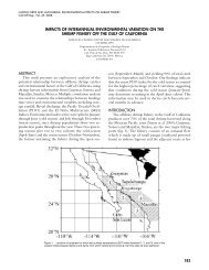
BINDMAN: 1985 NORTHERN ANCHOVY SPAWNING BIOMASSCalCOFl Rep., Vol. XXVII, 1986THE 1985 SPAWNING BIOMASS OF THE NORTHERN ANCHOVYANDREW G. BINDMANNational Marine Fisheries ServiceSouthwest Fisheries CenterP.O. Box 271La Jolla. California 92038ABSTRACTThe 1985 spawning biomass of the central subpopulationof the northern anchovy (Engradis rnordax) is522,000 metric tons (MT). This estimate was made usingthe egg production method, which computes thespawning biomass as the ratio of the daily egg productionrate (eggs per day for the entire population) and thedaily specific fecundity (eggs per day per metric ton).For the entire population, the egg production rate was16.95 x lo'* eggs/day, and the daily specific fecunditywas 37.00 X lo6 eggs/day/MT. In 1985 anchovyeggs were found farther offshore than in any surveysince the egg production method was first employed in1980. A significant number of eggs spawned far offshoremay have been missed by the survey, thus biasingthe estimate downward.RESUMENEn 1985, la biomasa de desove de la subpoblaci6ncentral de la anchoveta norteiia (Engradis mordax) es522,000 toneladas metricas (TM). Esta estimacion fuecalculada por medio del metodo de produccih dehuevos, 61 cual calcula la biomasa de desove como laproporcih entre la tasa diaria de produccion de huevos(huevos por dia para toda la poblacion) y la fecundidadespecifica diaria (huevos por dia por tonelada mktrica).La tasa de produccion de huevos de la poblaci6n totalfue 16.95 x 10I2 huevoddia, y la fecundidad especificadiaria 37 .OO X lo6 huevos/dia/TM. Los huevos deanchoveta fueron encontrados mas alejados de la costaen 1985 que en cualquiera de 10s estudios anterioresdesde que el metodo de produccion de huevos fuera inicialmenteempleado en 1980. Es posible que un numerosignificativo de 10s huevos puestos mar afuera hayasido obviado por el presente estudio implicando unasubestimacih de la biomasa.INTRODUCTIONThis estimate of the 1985 spawning biomass of thecentral subpopulation of the northern anchovy (Engraulisrnordux) fulfills the requirements of the AnchovyManagement Plan adopted by the Pacific FisheryManagement Council (PFMC 1983). In the past, an-(Manuscript received January 29, 1986.1chovy biomass has been estimated using a larval censusmethod (Smith 1972; Stauffer and Parker 1980;Stauffer and Picquelle 1981) and an egg productionmethod (Parker 1980; Stauffer and Picquelle 1980;Picquelle and Hewitt 1983, 1984; Hewitt 1984; Lasker1985). In 1985 only the egg production method wasused to estimate the anchovy spawning biomass.With the egg production method (EPM), we computethe spawning biomass as the ratio of the dailyproduction of eggs (eggs per day for the entire population)and the daily specific fecundity (eggs per day permetric ton) of the adult population. The daily productionof eggs is estimated from the density and embryonicdevelopmental stages of egg samples from an ichthyoplanktonsurvey. The developmental rates of anchovyeggs are measured in the laboratory under various temperatureregimes. The daily specific fecundity of theanchovy population is estimated from adult fish sampledduring a trawl survey. The parameters used toproduce the average specific fecundity are average femaleweight, batch fecundity, sex ratio, and theproportion of females spawning each night. Varianceand covariance values are also produced for theparameters.The survey results, the EPM estimate of spawningbiomass, and the variance of the estimate are presentedin the following sections.DESCRIPTION OF THE SURVEYThe 1985 EPM survey of the central subpopulationof northern anchovy was conducted with the NOAAship David Starr Jordan from January 28 throughMarch 8, 1985. The survey (Figure 1) ran from north tosouth starting approximately 50 miles south of Monterey,California, (CalCOFI line 71.7) and ending atBahia del Rosario, Baja California, (CalCOFI linellO.0). Several survey lines were extended farther offshorethan planned because of the unexpected extent ofpositive samples. The survey lines directly north of thegreatest concentration of anchovy eggs (northwest ofSan Diego) may not have extended far enough offshoreto sample the northern extent of this concentration.Thus a significant number of anchovy eggs may havebeen missed.We used a 25-cm-diameter vertical egg net with a0.15-mm mesh to take plankton samples from 70-m-16

BINDMAN: 1985 NORTHERN ANCHOVY SPAWNING BIOMASSCalCOFI Rep., Vol. XXVII, 19863936I 1 I l l 1 1 1 1 I 1> ANCHOVY%.an Francisco113...

BINDMAN: 1985 NORTHERN ANCHOVY SPAWNING BIOMASSCalCOFI Rep., Vol. XXVII, 1986The egg production method estimate of spawningbiomass (Parker 1980; Stauffer and Picquelle 1980) is:where B =P =w =R =F =s =A =k =B = PAkWRFSspawning biomass in metric tons,daily egg production rate in number ofeggs per day per 0.05 m2,average weight of mature females ingrams (g),female fraction of the population byweight,batch fecundity in number of eggs,fraction of mature females spawning perday ,area of survey in units of 0.05 m2, andconversion factor from grams to metrictons ( lop6 MT/g).An estimate of an approximate variance for thebiomass estimate, der&ed using the delta method(Seber 1982), is:var(B)Z= B2{var(P)/P2 + var(W)/W2 + var(R)/R2 +var(F)/F2 + var(S)/S2 + 2[cov(PW)/PW -COV(PR)/PR - COV(PF)/PF - COV(PS)/PS -COV(WR)/WR - COV(WF)/WF - COV(WS)/WS+ cov(RF)/RF + cov(RS)/RS + cov(FS)/FSI 1.DAILY PRODUCTION OF EGGSThe daily production of eggs in the sea, P, is thenumber of eggs spawned per night per unit area (0.05m2, the area of the ichthyoplankton net) averaged overthe range and duration of the survey. The density ofeggs was determined from an ichthyoplankton survey,and the embryonic developmental stage of each eggwas determined by microscopic inspection. The agesof the eggs in hours from spawning were computedfrom the embryonic developmental stage by aFORTRAN program (Hewitt et al. 1984; Lo 1985)which assumes that the daily spawning of anchovyeggs occurs at 2200 hours. An exponential mortalitycurve for the eggs was fit to the egg age data. I estimatedthe daily production of eggs as the value of thepredicted curve at the time of spawning.In order to reduce the variance of the estimate of P, Iused a two-step sampling scheme with postsurveystratification. The first step was the systematicichthyoplankton sample of the survey area. Each samplewas assigned a weighting factor proportional to the36.3330- -''21 I 1 I l l I I I I I I120 123 120 117 114Figure 4. Subdivision of 1985 survey into strata (stratum 1 is the spawningarea; stratum 0 is devoid of eggs).area the station represented. The second step was todivide the survey area into two strata: stratum 1 was definedas the area where eggs were found or were likelyto be found based on incidence in surroundinglocations, and stratum 0 was the area devoid of eggs(Figure 4).The egg mortality modelwas fit to the data by a weighted nonlinear leastsquaresregression, with station-weighting factors usedas the weights,where P,, = the number of eggs of age t from thejthstation in the ith stratum,t = the age in days measured as the elapsedtime from the time of spawning to thetime of sampling at thejth station (becausespawning occurs once a day andbecause the incubation period was 3days or less, as many as 3 cohorts ofeggs could be found at each station),Z = the instantaneous rate of mortality on adaily basis,PO = the daily egg production rate instratum 0; it is zero by definition, and18

BINDMAN: 1985 NORTHERN ANCHOVY SPAWNING BIOMASSCalCOFl Rep., Vol. XXVII, 1986PI = the daily egg production rate instratum 1.Mean half-day frequencies for the age data along withthe fitted curve and a 95% confidence region for theregression line are described in Figure 5. By definition,the number of eggs produced in stratum 0 is zero. Thedaily egg production rate for the total survey area andits variance (Jessen 1978) is:whereP = (Al/A) PI (4)var(P) = (1 + l/n)[(AI/A) var(P1)] (5)n = the total number of stations,AI = the area of stratum 1, andA = the total survey area.The estimates used to compute P, and their variancesare given in Table 1. P was found to be 6.41 withinstratum 1. For the entire 51,720 n.mi.2 survey area, theestimate of P is 4.78 eggs per day per 0.05 m2 with anapproximate variance of 0.33. This gives a coefficientof variation of 12.0%ADULT PARAMETERS W, F, S, AND RThe parameters W, F, S, and R were estimated from asample of adult anchovies collected by midwater trawl.For each parameter (here denoted y), a weighted mean,F, and a weighted variance were estimated (Cochran1963):wherevar6) = $i [(mi/m)2~j-y’>2]/[n(n-~~] (7)Imi = the number of fish subsampled fromthe ith trawl,fi = the average number of fish subsampledper trawl,n = the number of positive trawls,k ’z3a 6 .Wnv)00w 4U0aWm= 23z00.0 0.5 1 .0 1.5 2.0 2.5AGE (days)Figure 5. Egg mortality curve. The data are summarized as the meanabundance by half-day intervals, although the regression was fit to the individualdata points. A 95% confidence region for the regression (brokenlines) is indicated.-y, = the average value for the ith trawl = C.yjj/mj, andjyv = the observed value for thejth fish in theith trawl.Average Female WeightThe average weight of an adult female, W, and itsvariance were estimated using equations 6 and 7, whereyi was the average female weight in the ith trawl. I computedaverage female weight by selecting 25 maturefemales from each trawl; however, this was not alwayspossible because some trawl samples were too small orwere dominated by immature fish.Just prior to spawning, the eggs in a mature female’sovaries become bloated with fluid (hydrated). Icorrected for the extra weight of the hydrated eggs byregressing the weight of mature females without hydratedeggs against their ovary-free weight and then estimatingthe weight of the hydrated females as if theyTABLE 1Parameters for Computing Daily Egg ProductionStratum 0 Stratum I Total surveyP (eggs/day-0.05m2) 0 6.41 4.77var(P) 0 0.44 0.33Z (day- ’)var(Z)000.290.0070.290.007A (0.05m2) 0.904 X IO” 2.644 X IO’* 3.548 X 10l219

~~ ~BINDMAN: 1985 NORTHERN ANCHOVY SPAWNING BIOMASSCalCOFI Rep., Vol. XXVII, 19861520,000 -10>c0za15.000 -s 10,000 -YI0I-am5000 --AVERAGE FEMALE WEIGHT (a)Figure 6. Frequency distribution of average mature female weight per trawldid not contain hydrated eggs. The following regressionequation was found:nwhere Wk = - 0.3030 + 1.09 W* (8)= estimated weight in grams, andW* = ovary-free weight in grams.The regression was highly significant, with a significancelevel much less than 0.001. The frequency distributionfor average weight per trawl is described in Figure6. The average weight of a female for the entiresurvey, W, and its variance are listed in Table 2.Batch FecundityThe batch fecundity, F, for each mature female is theaverage number of eggs spawned per female at each0 " " 1 " " ~ " " ' ~ " ~ 1 " ' 1 " " ~ ~0 5 10 15 20 25 30OVARY-FREE WEIGHT (e)Figure 7. Linear regression of batch fecundity on ovary-free weight fit to 85females with hydrated ovaries.spawning event. The batch fecundity was estimated foreach female fish by a two-step process. The first stepwas a regression of batch fecundity versus ovary-freeweight from a sample of 85 hydrated females (Figure7). The ovary-free weight distribution of these 85 fishwas similar to the ovary-free weight distribution of allmature females (Figure 8). The estimated regressionequation was:= - 2035.6 + 682.1 W" (9)where = the estimated fecundity for a female withW* ovary-free weight. The regression was highlysignificant, with a significance level less than 0.001,The second step was to estimate the batch fecundity foreach mature female fish from its ovary-free weight andthe above regression. I estimated the average batch fecundityfor the entire survey area by using equation 6where yij = ku, the estimated batch fecundity; the de-TABLE 2Estimates of Egg Production Parameters, Variances, and Coefficients of VariationCoefficientParameter Value Variance of variationDaily egg production (eggs/day) (PA) 16.95 X 10" 4.11 X 15.6%Average female weight (g)Batch fecundity (eggs)Spawning fraction (day- I)Female fractionDaily specific fecundity ( IO6 eggsiday -MT)(W 14.494 0.105 2.2(F) 7,343. 1.145 X IO5 4.6(9 0.120 0.00024 12.9(R 1 0.610 0.00038 3.237.003Spawning biomass (MT) (not including San Francisco area) (B) 458,024 7.374 x 109 18.7Spawning biomass (MT) (including San Francisco area) (B) 522,00020

BINDMAN: 1985 NORTHERN ANCHOVY SPAWNING BIOMASSCalCOFI Rep., Vol. XXVII, 1986500 r400L$ 300w3[ 200100025 cOVARY-FREE WEIGHT (9)sired mi was 25 females. The variance equation (7) wasmodified because of the extra source of variation fromthe fecundity/ovary-free weight regression (Draperand Smith 1966):var(r) = C (mj/fi)2[(Fj-F)2/(n-l) + S1,'/85i + (w;*-ivh*)2var(b)]/n (10)where sh2 = 3,748,191 is the variance about the re-- gression,W,* = average ovary-free weight for the ith- traw 1,wh* = 15.43 g, average ovary-free weight ofthe 85 hydrated females used in the regression,vir (b) = 2,453, variance of the slope of the regression,andn = 63, the number of positive trawls.The average batch fecundity and its variance appear inTable 2.OVARY-FREE WEIGHT (g) (Regression)Figure 8. Frequency distributions of ovary-free weight for the entire survey(top) and for the females with hydrated ovaries used to estimate the batchfecundityiovary-free weight regression.Spawning FractionThe spawning fraction is the proportion of maturefemales that spawned on the night prior to capture(day-1 spawners). The spawning fraction, S, and itsvariance were estimated using equations 6 and 7 whereyi = Si was the spawning fraction found from the ithtrawl. The desired mj-the sample size pertrawl- was 25. Strong evidence indicates that femalesspawning on the night of capture (day-0 spawners) areoversampled by the trawl (Picquelle and Hewitt 1983).To account for this, I adjusted mi by assuming thatthere was an equal incidence of day-0 and day-I30 spawning fish and hence substituting the day- 1spawners for the day-0 spawners. The frequency distri-25bution of the spawning fraction appears in Figure 9.The estimate of S and its variance are found in Table 2.20> Female Fraction0zThe female fraction of the population by weight isWa 15the parameter R. Equations 6 and 7 were used where yjs a= Ri, the total weight of females in a subsample of ap-U.proximately 50 fish divided by the total fish weight.10For each trawl, average weights of male (n = 5) and female(n = 25) fish were measured, and the weights of5hydrated females were adjusted using the regressiongiven in equation 8. These average weights were usedto estimate the total female weight and the total fish0o 0.05 0.10 0.15 0.20 0.25 0.30 0.35 0.40 0.45 weight. The frequency distribution of R is givenPROPORTION OF DAY-1 SPAWNERSin Figure 10; the estimate and variance are shown inFigure 9. Frequency distribution of spawning fraction.Table 2.21

BINDMAN: 1985 NORTHERN ANCHOVY SPAWNING BIOMASSCalCOFI Rep., Vol. XXVII, 198618rL2; = number of larvae caught at each stationin region 2, andAi = area represented by station i.The final biomass estimate for the survey area plus thenorthern area was 458,025 + 63,718 = 521,742 MT.The variance of this estimate was not computed. However,the coefficient of variation is certainly larger thanthe 19% associated with the entire region of the EPMsurvey (Table 2).PROPORTION FEMALE BY WEIGHTFigure 10. Frequency distribution of female fraction by weight.BIOMASS ESTIMATE AND VARIANCEUsing equations 1 and 2, I estimated the spawningbiomass for the portion of the population range coveredby the survey to be 458,025 MT, with a standard errorof 85,872 MT. This gives a coefficient of variation of18.75% The values of the parameters that were used inthe estimate, and their variances and covariancesappear in Tables 2 and 3. The northern part of thepopulation range was not covered by this survey.The results of the Mys Babushkina cruise show that,as in past years, there is spawning off San Francisco.The Soviet cruise covered the area from Point Conception(CalCOFI line 80.0) north to line 70.7-thenorthern extent of our biomass survey (region 2)-aswell as the region north of line 70.7 (region 1). TheSoviets used a bongo net to collect anchovy eggsand larvae. Because larvae are less patchy than eggs, Iused “scanned” larvae counts (Figure 3) as an indicatorof relative spawning biomass in the two regions. Specificfecundity and subsequent mortality rates ofeggs and larvae are assumed to be constant throughoutthe spawning area. The biomass of region 1 was calculatedas:B1 = B2*where B1 =B2 -Llj -2 (Ll; * Ai)C (L2; * A;)1= 63,718MTestimated spawning biomass of region1,29,090 MT is the spawning biomass ofregion 2 (biomass equation),number of larvae caught at each stationin region 1,DISCUSSIONThe 1985 egg production method estimate of thespawning biomass of the central subpopulation of thenorthern anchovy is up by 61% from its lowest point(since 1980) in 1984. Table 4 lists the historical time seriesof parameters. The change in spawning biomass iscaused by a 3 1 % increase in egg production and a 13%increase in the daily specific fecundity from 1984. Thedecrease in daily specific fecundity results from a dropin the spawning fraction to a level average for 1980-84and an increase in batch fecundity. The larger batch fecundityis strongly related to a 21 % increase in femaleweight, because the two are highly correlated (Table3). The ratio of batch fecundity and mean weight (FIW)estimates the specific batch fecundity (Table 4). The increasein this ratio is less than the rise in batch fecundity,implying that much of the growth in batch fecundityis due to a larger average female weight. The egg mortalityrate Z was higher this year than it has been since1980. The very large 1980 rate, along with this year’shigh Z value, demonstrates the variability of Z. Femalefraction remained very high compared to the yearsbefore 1984. The daily specific fecundity is lower than1984 but is still above the average for 1980-83.The EPM spawning biomass estimate can be comparedto an annual acoustic survey, which provided ameasure of total anchovy biomass. The California Departmentof Fish and Game conducted an acoustic andmidwater trawl survey of the northern anchovy in February1985 (Cruise Report 85-X-1 , K.F. Mais, CDFG,Long Beach, California). The cruise was restricted tothe area between Point Conception (CalCOFI Iine80.0) and the U.S.-Mexican fishery boundary. Inagreement with our results, Mais reports that the geographicdistribution of anchovies was more offshoreTABLE 3Covariances between Adult ParametersF S Female fraction (R)Female weight (W) 66.25495 0,00076 0.00064759Batch fecundity (F) 0.53235 0.44352668Spawning fraction (S) 0.0000553122

BINDMAN: 1985 NORTHERN ANCHOVY SPAWNING BIOMASSCalCOFI Rep., Vol. XXVII, 1986TABLE 4Time Series of Egg Production Parameters (1980-85)Daily egg production ( I 012 eggsiday)I980 1981 I982 1983 1984 1985“26.34 20.96 13.51 17.25 12.98 16.95Egg mortality rate0.450.140. I60.18 0.170.29Average female weight (g)17.4413.3718.8311.20 12.0214.50Batch fecundity (eggs)7,7518,32910,8455,297 5,4857,343Spawning fraction0. I420. I060.1200.094 0.1600.120Female fraction0.4780.5010.4720.549 0.5820.609Daily specific fecundity ( IO6 eggs/day/MT)30.2833.0332.5324.35 42.4337.00Specific batch fecundity (eggdg)444623576473 456506Spawning biomass (10’ MT)870635415652 309522’Coef. of variation for (B)0.260.220.060.21 0.170.19”Calif. Dept. Fish and Game498 493 233 46 1 479acoustic biomass estimateto to to to tof , nj MT)1 v I. - -, 598 59 1 247 504 560’Does not include San Francisco area’Includes San Francisco‘Does not include Mexican portion of anchovy population627to753‘and southward than in any other survey year. He alsoreported that the bulk of the population was “located inan arc of 80 miles west to south, and 30 miles east tosouth of San Clemente Island.” This is where oursurvey found the greatest density of anchovy eggs (Figure1). Mais calculated the total biomass of anchovies(not spawning biomass) to be 627,000-753,000 MT inU.S. waters off southern California. This is up 30.8%-34.5% from his results of 1984. He concludes thatthe 1985 estimate is the highest in five years andthat it would have been higher if the proportion of theanchovy population located in Mexican waters beenincluded.In previous years the survey area was divided intoregions in order to reduce the variance of the parametersand the variance of the biomass estimate (Picquelleand Hewitt 1983; Hewitt 1984). The regionalizationwas indicated because there were significantdifferences in one or more parameters betweenregions. There is no indication that regionalizationwould have reduced the variance of this year’sestimates.Anchovy eggs were found much farther offshorethan in any year since the egg production methodsurveys began in 1980. A large number of eggs far offshoremay have been missed by our survey. Asmentioned earlier, if a significant number were missed,there would be a downward bias in our biomass estimate.ACKNOWLEDGMENTSA. MacCall of the Southwest Fisheries Center(SWFC) coordinated this year’s biomass estimate. Wewould like to sincerely thank all those who took part inthis year’s project. J. Hunter, R. Lasker, G. Moser, andJ. Thrailkill of SWFC, and L. Farrar of SWFC and theNational Ocean Service directed the field collections,laboratory processing, and data analysis. The cruisewas conducted by the crew of NOAA ship David SturrJordan with its captain M. Roll. W. Flerx (SWFC) ledthe team of scientists participating on the cruise: theywere, from SWFC, D. Abramenkoff, D. Ambrose, P.Arenas, J. Butler, and E. Lynn; and, from Mexico, A.Cota, F. Diaz, I. Vomend, and G. Vueltiflor. Laboratoryprocessing of the samples was by L. Dunn, M.Farrell, J. Haddox, A. Lumpkins, and F. Pocinich ofScripps Institution of Oceanography (SIO), and by D.Ambrose, M. Busby, D. Gruber, E. Lynn, B.Macewicz, B. MacCall, P. Paloma, E. Sandknop, andE. Stevens of SWFC. N. Lo and P. Smith (SWFC)provided advice, and N. Lo’s program was used to assignages to the eggs. R. Ford (SWFC) entered the data,and R. Charter (SWFC) and Cindy Meyer (SWFC)produced the computer graphics. Roy Allen (SWFC)23

BINDMAN: 1985 NORTHERN ANCHOVY SPAWNING BIOMASSCalCOFI Rep., Vol. XXVII, 1986drafted the final figures. Julie Shoemaker (SWFC)provided clerical help.LITERATURE CITEDCochran, W.G. 1963. Sampling techniques. John Wiley and Sons, NewYork, 413 p.Draper, N. R., and H. Smith. 1966. Applied regression analysis. JohnWiley and Sons, New York. 407 p.Hewitt, R.P. 1984. The 1984 spawning biomass of the northern anchovy.SWFC Admin. Rep. LJ-84-18, 17 p.Hewitt, R.P., A.G. Bindman, and N. Lo. 1984. Procedures for calculatingthe egg production estimate of spawning biomass. SWFC Admin. Rep.LJ-84-19,46 p.Jessen, R.J. 1978. Statistical survey techniques. John Wiley and Sons, NewYork, 500 p.Lasker, R., ed. 1985. An egg production method for estimating spawningbiomass of pelagic fish: application to the northern anchovy (Engruulismordux). U.S. Dep. Commer. NOAA Tech. Rep. NMFS 36,99 p.Lasker, R., J. Pelaez, and R.M. Laurs. 1981. The use of satellite infraredimagery for describing Ocean processes in relation to spawning of thenorthern anchovy, Engruulis mordux. Rem. Sens. Environ. 11:439-453.Lo, N. 1985. A model for temperature-dependent northern anchovy eggdevelopment and an automated procedure for the assignment of age tostaged eggs. In R. Lasker (ed.), An egg production method for estimatingspawning biomass of pelagic fish: application to the northern anchovy(Engruulis mordar). U.S. Dep. Commer. NOAA Tech. Rep. NMFS 36,99 p.Parker, K. 1980. A direct method for estimating northern anchovy.Engruulis mordux, spawning biomass. Fish Bull., U.S. 78541-544.PFMC: Pacific Fishery Management Council. 1983. Northern AnchovyFishery Management Plan. PFMC, 526 S.W. Mill St., Portland, Oregon97201.Picquelle, S.J., and R.P. Hewitt. 1983. The northern anchovy spawningbiomass for the 1982-83 California fishing season. Calif. Coop. OceanicFish. Invest. Rep. 24:16-28.-. 1984. The 1983 spawning biomass of the northern anchovy. Calif.Coop. Oceanic Fish. Invest. Rep. 25:16-27.Seber, G.A.F. 1982. The estimation of animal abundance. Macmillan, NewYork, 654 p.Smith, P.E. 1972. The increase in spawning biomass of northern anchovy.Engruulis mordux. Fish Bull., U.S.,70:849-874.Stauffer, G.D. 1980. Estimate of the spawning biomass of the northemanchovy central subpopulation for the 1979-80 fishing season. Calif.Coop. Oceanic Fish. Invest. Rep. 21:17-22.Stauffer. G. D., and K. Parker. 1980. Estimate of the spawning biomass ofthe northern anchovy central subpopulation for the 1978-79 fishingseason. Calif. Coop. Oceanic Fish. Invest. Rep. 21:12-16.Stauffer, G.D., and S.J. Picquelle. 1980. Estimates of the 1980 spawningbiomass of the central subpopulation of northern anchovy. SWFC Admin.Rep. LJ-80-09,41 p.-- . 1981. Estimate of the spawning biomass of the northern anchovycentral subpopulation for the 1980-81 fishing season. Calif. Coop.Oceanic Fish. Invest. Rep. 22:8-13.24

WOLF AND SMITH: MAGNITUDE OF SARDINE SPAWNING BIOMASSCalCOFI Rep., Vol. XXVII, 1986THE RELATIVE MAGNITUDE OF THE 1985 PACIFIC SARDINE SPAWNINGBIOMASS OFF SOUTHERN CALIFORNIAPATRICIA WOLFCalifornia Department of Fish and Game245 West BroadwayLong Beach, California 90802PAUL E. SMITHNational Marine Fisheries ServiceSouthwest Fisheries CenterP.O. Box 271La Jolla, California 92038ABSTRACTThe spawning biomass of the Pacific sardine offsouthern California during 1985 is considered to be atleast 20,000 short tons’. This determination was madeusing an inverse egg production or “egg productionarea” method, which estimates the area over which aspecified spawning biomass (20,000 tons) would beexpected to occur. Our survey had a 95% probability ofdetecting the spawning area within the survey area if atleast 20,000 tons of adults were present. This methodwas developed from the egg production method,which estimates adult biomass from measurements ofegg production in the spawning area and from the eggproduction rate of the adult population. Using estimatesof the components of egg production and specificfecundity for sardines from previous studies, wepredicted that 20,000 tons of spawning biomass wouldcover a spawning area of about 500 n.mi2.A total of 86 sardine eggs was collected at 11 of 419stations during the May 1985 survey, which rangedfrom San Diego to Point Conception and extendedfrom within one mile of the coast to approximately 80miles offshore. Spawning occurred mainly along theSanta BarbardVentura coast and covered an estimated670 n.mi2. A total of 1,170 anchovy eggs and 266 anchovylarvae were found at 114 and 69 of the stations,respectively.As provided by state law when the sardine biomassreaches 20,000 tons, a 1,000-ton fishery for sardineswas opened on January 1, 1986. This is the first directedfishery allowed for California sardines since amoratorium on sardine fishing was enacted in 1974.Adult reproductive parameters and egg survival mustbe determined for absolute biomass estimation.RESUMENLa biomasa de desove de la sardina del Pacific0frente a1 Sur de California fue estimada en por lo menos20,000 toneladas cortas (1 tonelada corta = 0.907[Manuscript received February 14, 1986.1’ Commercial landings, tonnages specified in legislation. and tonnages in this paperare reported in short tons.toneladas metricas) en 1985. Esta determinacion fuehecha por medio del mCtodo inverso de produccion dehuevos o “area de produccion de huevos.” Este metodoestima el area en la cual una biomasa de desove dada(20,000 toneladas) supuestamente tendra lugar.Nuestro estudio permitiria localizar el area de desovedentro del &-ea de estudio con un 95% de probabilidadsi hubieran, al menos, 20,000 toneladas de adultos.Este mCtodo esta basado en el metodo de produccion dehuevos el cual evalua la biomasa de adultos a partirde medidas de la produccion de huevos en el area dedesove, y de la tasa de produccion de huevos por lapoblacion de adultos. Sobre la base de estudios previossobre la produccion de huevos y la fecundidad especificade las sardinas, se pronostican 20,000 toneladas debiomasa de desove en un &-ea de desove de alrededorde 500 mi.n2.Se colectaron 86 huevos de sardinas en 11 de 419estaciones ubicadas entre San Diego y Point Conception,y que se extendian entre 1 y aproximadamente 80millas mar afuera, durante mayo de 1985. El desoveocurrio a lo largo de la costa entre Santa Barbara y Venturaprincipalmente, cubriendo un area estimada en670 mi.n2. Se encontraron 1,170 huevos y 266 larvas deanchoveta en 114 y 69 de las estaciones, respectivamente.De acuerdo con la legislacion estatal, cuando la biomasade sardina alcanz6 20,000 toneladas, se abri6 unapesqueria para 1,000 toneladas de este recurso el 1 O deenero de 1986. Esta es la primera pesqueria dirigidaque se permite para las sardinas de California desde laimplementation, en 1974, de una Veda de esta pesqueria.Para obtener una estimacidn absoluta de la biomass,10s parametros reproductivos de 10s adultos y lasobrevivencia de 10s huevos deben ser determinados.INTRODUCTIONThis report assesses the 1985 spawning biomass ofthe Pacific sardine. Legislation closing the sardinefishery in 1974 requires the Department of Fish andGame to determine annually whether the spawningbiomass is more than 20,000 tons. This legislation imposesa moratorium on fishing sardines while the biomassremains below 20,000 tons and allows a 1,000-25

WOLF AND SMITH: MAGNITUDE OF SARDINE SPAWNING BIOMASSCalCOFl Rep., Vol. XXVII, 1986ton fishery when the biomass exceeds this level.Earlier assessments of the sardine spawning biomasswere based on ichthyoplankton surveys, aerial observations,trawl surveys, and incidental landings inmackerel and live bait fisheries, and have shown signsof increase since 1980 (Wolf 1985; Klingbeil and Wolf1984; Klingbeil 1981, 1982, 1983).Because the sardine population appeared to increase,a quantitative method for detecting recoveryand determining whether the biomass had exceeded20,000 tons was required. Estimates of the sardinepopulation biomass during the fishery were based onanalysis of catch and age data (Murphy 1966; MacCall1979). The egg production method (Parker 1980) iscurrently used to estimate spawning biomass of anchoviesoff California (Picquelle and Hewitt 1983) and anchoviesand sardines off Peru (Santander et al. 1982).However, available methods of biomass estimation arenot applicable at low biomass levels; the cost and effortnecessary to achieve meaningful levels of precision aretoo high.We developed the egg production area method to allowa cost-efficient, quantitative determination of therelative magnitude of spawning biomass while levelsremain low. Details of the method and survey designare described by Wolf and Smith (1985). Here we applythe egg production area method to assess the relativemagnitude of the sardine spawning biomass during1985.EGG PRODUCTION METHODThe egg production method estimates spawningbiomass asB kw= PoA-RFSwhere B = spawning biomass (MT)Po = daily egg production, number of eggsproduced per 0.05 m2 of sea-surface area,W = average weight of mature females (g),R = sex ratio, fraction of population that isfemale, by weight (g),F = batch fecundity, number of eggs spawnedper mature female per batch,S = fraction of mature females spawning perday,A = total area of survey (0.05 m2), andk = conversion factor from grams to metrictons.This method was derived by Parker (1980), and appliedby picquelle and Hewitt- (1983, 1984) and Hewitt(1985) to estimate northern anchovy biomass.EGG PRODUCTION AREA METHODIn the egg production method, daily egg productionand population fecundity parameters are measured duringthe survey. An exponential mortality model is fit tocounts of aged eggs, and Po is estimated by extrapolatingback to the number of eggs at the time of spawning.Parameters W, F, S, and R are estimated from samplesof adult fish collected during the survey.In the egg production area method, the spawningbiomass is specified and the equation solved for A I :BIRFSmAi =Pok, wwhere A, = spawning area of biomass B1 in nauticalmiles2,B, = spawning biomass, in short tons,kl = conversion factor from grams to tons,m = conversion factor from 0.05 m2 to nauticalmiles2.The procedure for estimating sardine spawning areadiffers from that used for anchovy2 in that occasionalstations with no eggs are incorporated for anchovy: aslight increase in area is compensated by a slight decreasein mean abundance of eggs. For the sardinespawning area estimate, only stations with eggs are included.We assumed that an area represented by asingle sample is not entirely covered, but that this iscompensated by the fact that eggs might be presentin another area represented by a sample containingno eggs.We used information from previous studies to estimatethe parameters, Po, W, F, S, and R for sardinesrather than collecting measurements during the survey.These values (Table 1) are not known or have not beenmeasured recently for California sardines; we adaptedexisting information concerning sardines and relatedspecies (Wolf and Smith 1985).Estimates of daily egg production for sardines andanchovies off Peru3 indicate that egg production ratesare lower for sardines than for anchovies by a factor of1:2. We applied this relationship to annual estimatesfrom 1980 through 1984 (Hewitt 1985) of daily eggproduction rates for anchovies (approximately 10 eggs/0.05 m2) to obtain an estimate of sardine daily egg productionof about 5 eggs/0.05 m2. Historical CalCOFIegg surveys yielded an estimated California sardinedaily egg production rate of approximately 1.5 eggs/0.05 m2. This value is thought to be low, however, be-' La\ker, R (ed ) MS An egg production method for estimating spawning biomass ofpelagic fish application to the northern anchovy (Engrauhsrnordax)Smith, P.E., H. Santander, and J. Alheit. MS. Comparison of the monality and dispersalof sardine (Sardinops sagm sugar) and anchovy (Engradis ringens) eggs offPeru.26

WOLF AND SMITH: MAGNITUDE OF SARDINE SPAWNING BIOMASSCalCOFI Rep., Vol. XXVII, 1986TABLE 1Parameters Used to Estimate Spawning Area, and Resulting EstimatesBI W R F P., S A,Spawning biomass Average female Sex ratio Batch fecundity Egg production~Spawning fraction~~Spawning area(short tons) weight (8) (femalesitotal) (eggsibatchi (eggs/.05m’-day) (spawning females/ (nautical miles’)female)total females)20,000 120 0.5 32,000 5.0 0.020.050.100.151413537061,0581.5 0.020.050.100.15470I, I762,3523.528cause the sampling technique (oblique tows instead ofvertical tows) may have overestimated the surface areaof water sampled. Both values of P, were used (Table1). Average weight of mature females, W, was estimatedto be 120 grams, and batch fecundity, F, was estimatedat 32,000 eggs (MacGregor 1957). The femalefraction of the population by weight, R, was assumedto be half. Spawning fraction, S, for other pelagic speciesranges from 0.02 females spawning per day(spawning once every 50 days) for Pacific sauries(Hatanaka 1956) to 0.14 females spawning per day(spawning once every 7 days) for anchovies (Hunterand Macewicz 1980). Spawning fraction for sardinesoff Peru (J. Alheit, Instituto del Mar del Peru, pers.comm.) and for sardines off the west coast of Baja California(J.R. Torres-Villegas, CICIMAR, unpublisheddata) has been estimated at about 0.06 females spawningper day. The range values of S was used (Table 1).The calculated area, A,, over which 20,000 tons ofPacific sardines could be expected to spawn rangesfrom 141 to 1,058 n.mi.2, for an estimated daily eggproduction rate of 5 eggd0.05 m2 and an estimatedrange of values for spawning fraction, and from 470 to3,525 n.mi.2 for a daily egg production rate of 1.5 eggs/0.05 m2 and the same range of values for spawningfraction (Table 1). With available information, we considerthe higher value of P,-5.0 eggs/0.05 m2-and avalue of S ranging between 0.05 and 0.10 femalesspawning per day to be the best estimates of these parametersfor sardines. Therefore, 500 n.mi.2 was selectedas a useful estimate of A I .SURVEY DESIGNThe survey area and time of year over which sardinespawning would be likely to occur were determinedfrom occurrences of sardine eggs and larvae in historicalCalCOFI survey data (Wolf and Smith 1985). Thecritical spawning area, A,, estimated at 500 n.mi.*,was approximately 2% of the survey area, which in-cluded CalCOFI regions 7 and 8 and covered an estimated32,000 n.mi.2 (Smith et al. 1976). Using a tablefor determining confidence limits of a proportion (Natrella1963), we determined the number of stations(374) representing the minimum effort required to locatethe spawning area within the survey area, with ahigh probability (95%) of detecting the spawning areaif 20,000 tons of spawning adults were actually present.The stations were spaced 4 n.mi. apart offshoreand 10 n.mi. apart alongshore according to standardanchovy egg production procedures. Because each stationrepresents 40 n.mi.*, the calculated spawning areathat 20,000 tons of sardines would cover was expectedto contain 12 or 13 positive stations.SURVEY DESCRIPTIONThe survey was conducted by NOAA ship DavidStarrJordan from April 29 through May 19, 1985. Stationswere occupied from south to north, beginning atSan Diego and ending at Point Sal, and extending offshorean average distance of about 80 miles (Figure 1).Plankton samples were collected at 419 stations using a25-cm-diameter CalVET (vertical egg tow) net of 150-micron mesh that was retrieved vertically from 70 m(when depth allowed) to the surface. Samples werecollected at all hours. No stations were occupied in establishedshipping lanes.Sardine and anchovy eggs and larvae were identified,sorted, and counted. A total of 86 sardine eggsoccurred at 11 stations, with the number of eggs perstation ranging from 1 to 42 (Figure 2). Most of thepositive stations occurred along the coast near SantaBarbara, and in the eastern portion of the Santa BarbaraChannel, from Port Hueneme to Anacapa and SantaCruz islands. Two positive stations occurred off NewportBeach. Sardine larvae occurred at 10 stations, inapproximately the same areasas eggs. Eggs and larvaein combination occurred at 16 stations.Evidence of anchovy spawning (1,710 eggs and 26627

WOLF AND SMITH: MAGNITUDE OF SARDINE SPAWNING BIOMASSCalCOFI Rep., Vol. XXVII, 198636 - \ SARDINE SURVEY I33 - PT.123 120 117Figure 1. Stations occupied during sardine survey, May 1985.larvae at 114 and 69 stations, respectively) was considerablymore common but occurred in different areasthan sardine spawning. Anchovy eggs and larvae wereconcentrated mostly in the southern portion of the surveynear San Diego.Two of the samples had to be discarded because ofinadequate preservation. Neither were adjacent to ornear stations at which sardine eggs occurred (Figure 2).SPAWNING AREASpawning area was determined by multiplying thenumber of egg-positive stations by the area representedby each station (40 n.mi.*). Some stations that werepositive for sardine eggs were adjacent to areas thatwere not sampled, either because the area occurred inthe shipping lanes or was close to shore and aligned insuch a way that the station plan did not call for a sample.In order to consider these areas in the spawningarea estimate, we adjusted the area of positive stationsadjacent to an unsampled area to include half of the adjacentunsampled area, averaged along lines in order ofstation occupation and estimated by eye. The area ofpositive stations too near to shore to include an entire40 n.mi.2 were also adjusted to reflect the portion of the4 by 10 n.mi.* actually sampled.An unadjusted estimate of the spawning area equals440 n. mi2. An estimate of the spawning area adjustedas described above is 670 n.mi.* (Figure 2). Both ofthese estimates are within the range of spawning areacalculated for 20,000 tons of spawning biomass ofsardines and are close to the selected estimate of AI(Table 1).DISCUSSIONThe egg production area method allows detectionof the onset of sardine recovery and provides an objective,quantitative technique for determining therelative magnitude of spawning biomass. This is particularlyuseful when the management plan requires determiningwhether a specified spawning biomass levelhas been exceeded, but either the level to be ascertainedremains low enough that developing a directestimate with reasonable precision is cost- and effortprohibitive,or information beyond the relative magnitudeof biomass is unnecessary.Because the spawning area observed during the surveywas close to that predicted for 20,000 tons of adultsardines, the spawning biomass of sardines off Californiais considered to be at least 20,000 tons in 1985.As specified by state law, this determination allowedthe initiation of a 1,000-ton fishery in January 1986.The provision for a fishery was included in the 1974moratorium legislation because of concern that a totalmoratorium would preclude detecting the onset of recovery.Also, simulations of a 5% fishery at that biomasslevel projected no deleterious effects (W. Lenarz,NMFS, Tiburon, pers. comm.). MacCall’s (1979) estimatesof apparently lower recruitment rates at low biomasslevels suggest that Lenarz’s projections may beoptimistic.The large range of values calculated for A I resultedfrom using a range of values to estimate parameters P,(daily egg production rate) and S (spawning fraction).These parameters are not known for Pacific sardines.Two other parameters- W (average female weight)and F (batch fecundity)-were estimated from sardinestaken from the 1945-46 commercial catch. Theaverage monthly mean weight of mature female sardinesoccurring incidentally with mackerel during1985 was 142 grams. As discussed below, all of thecomponents of egg production and specific fecundityare dynamic and have been shown to vary from year toyear for northern anchovy (Hewitt 1985). Daily eggproduction rate and spawning fraction must be determinedfor Pacific sardines; the adult parameters shouldbe obtained simultaneously. The egg production areamethod, however, uses historical information.28

WOLF AND SMITH: MAGNITUDE OF SARDINE SPAWNING BIOMASSCalCOFI Rep., Vol. XXVII, 1986120119 118343:Figure 2 Number of eggs per station and location of stations that contained sardine eggs Rectangles outline 4-by-10-n mi areas represented by each station toillustrate spawning area adjustment Shaded area is adjusted sardine spawning area Open circles are discarded samplesSeveral other sources provide additional informationconcerning the status of the adult Pacific sardinepopulation during 1985. Incidental landings of sardineswith mackerel during 1985 totalled 652 tons, thelargest annual take in 20 years (“Review of Some CaliforniaFisheries for 1985 ,” this volume). Sardines havebecome increasingly more common in mackerel landings,occurring in 50% of observed landings in 1985compared to 30% in 1984. Catch length frequencies ofincidental sardines show a trend from 1983 through1985 of a broader length distribution, indicating recruitmentin 1985 (Figure 3). Sardines from the 1985year class were detected in early 1966 in MontereyBay, indicating that spawning occurred north of PointConception and beyond the range of the survey. Sardinesranked first in biomass and third in abundance inpurse seine hauls from Long Beach Harbor during 1983and the first half of 1984 (C. Mitchell, MBC AppliedEnvironmental Sciences, pers. comm.). No detectabletrend, however, was observed in the mean number ofsardines captured by purse seine off San Onofre from1983 through 1985 (E. DeMartini, UCSB FishProgram, pers. comm.).The abundance of sardine eggs and larvae in fournearshore ichthyoplankton transects in the SouthernCalifornia Bight increased two to three orders of magnitudefrom 1978-79 through 1982-84, and sardinesranked third in overall abundance during that period(R. J . Lavenberg , Los Angeles County Natural HistoryMuseum, pers. comm.). From 1978 through 1984,monthly mean numbers of sardine larvae in coastalwaters near San Onofre increased steadily (W. Watson,Marine Ecological Consultants of Southern California,pers. comm.). Both of these studies indicate that a sub-29

WOLF AND SMITH: MAGNITUDE OF SARDINE SPAWNING BIOMASSCalCOFI Rep., Vol. XXVII. 198626120-16-10-6-z 20'W2) 1 6 -0WLL10-6-II19831984N : 881N : 245ae I I 1120 140 180 180 200 220 240 200261610-6-1985N : 5 88I I120 140 180 180 200 220 240 280STANDARD LENGTH (MM)Figure 3 Catch length frequencies of sardines landed incidentally withmackerel in 1983, 1984, and 1985 Mean weights of modal length classesforeach year are 1983, 130 g. 205-209 mm SL, 1984, 147 g. 210-214 mm SL,1985,143 g, 205-209 mm SLstantial portion of sardine spawning in recent years hasoccurred relatively near to shore (within the 75-m contour)and during summer and fall.Although the limited interpretation of the 1985 surveyis conclusive in the original objectives relative to20,000-ton spawning biomass, we resist broadeningthese few results for a biomass estimate or fisheryquota. The spawning area of 670 n.mi.* is nearly identicalto the 500 n.mi.* criterion adopted for this tech-nique. This means that any deviation from the assumedadult parameters could change the evaluation. Anothercritical feature is that we can estimate only the standingcrop of eggs from this small set, not the egg production.The two unevaluated factors are mortality rate ofthe eggs and the precision of the intercept estimate. Futuresurveys must quantify the mortality rate and thefrequency distribution of eggs.The estimated mean of positive samples in the 1985survey is high relative to samples of the 1930s to 1950s(Table 2). It appears that the high value is due to thechance encounter of more observations with highvalues. We believe the cause of this difference istechnical rather than biological, although this cannotbe determined from these few samples. It is importantto note that all the other distributions result fromoblique or horizontal tows and that the new results arefrom a vertical tow. The scale of the integration is 25cm for the CalVET net and on the order of meters for allbut one of the other nets, and kilometers for the highspeednet used in 1950. The smaller CalVET net willhave a greater probability of sampling zero eggs. Also,the sampling threshold of the CalVET net (1 egg in aCalVET is equivalent to 50 eggs in a 1 -m oblique tow)might cause the lower end of the frequency distributionof egg densities to be undersampled. Both of thesecharacteristics would cause the mean observed densityof positive samples to be inflated. This would implythat the entire area of sardine spawning was notdetected and that 20,000 tons is a conservativeestimate.The high mean value could also result from a lowerthan normal mortality or higher than normal per capitaegg production rate, which would imply a lowerspawning biomass. These biological factors will allhave to be separately assessed for the absolute biomassto be estimated from egg production rates.Analogous data from the anchovy egg productionprocedure indicate the great importance of the adultsampling effort for biomass estimation. If the intervalbetween batches of eggs is long, for example 20 days,the ratio of gonads with evidence of spawning in theprevious day is only 5%. This ratio would requiremany independent samples to precisely determine thespawning fraction. Individual samples of anchovy femalesrange from 0% spawning to over 40% when themean is 15%. Thus the overall precision of spawningbiomass estimates may be determined by the ability toobtain a sufficient number of independent samples ofadult females.In summary, at least one more year of field andlaboratory work on additional egg samples and adultcollections will be required before the procedure for anabsolute biomass estimate can be designed.30

WOLF AND SMITH: MAGNITUDE OF SARDINE SPAWNING BIOMASSCalCOFI Rep., Vol. XXVII, 1986TABLE 2Pacific Sardine Egg Sample Frequency Distributions at Different Levels of Spawning BiomassaNet types and years#/IO m2CalVET CF&G 2-m 1 -m 0.5-m Hi-speed 1 -mx In(.x) 1985 1931-32 1941 1941 1950 1959.I25 -2.08 - b2 - - - -.5 -0.69 -4 - - - -2 0.69 -6 21- -288 2.08 - 7 22 8 -2832 3.47 - 14 16 15 -30128 4.85 4 12 31 29 77 23512 6.24 4 13 27 14 20 122,048 1.62 2 5 17 10 7 58,192 9.01 1 2 3 2 1 4Estimatedmean 1,564 544 569 619 406 410Biomass (MT)' 0.02 3.9 2.7 2.7 1 .0 0.2"(Smith and Richardson 1977)'Value below sampler threshold'(Murphy 1966)ACKNOWLEDGMENTSWe would like to acknowledge the editorial assistanceof two anonymous reviewers. Rocky French andTerry Palmisano helped with graphics. We thank thecrew of NOAA ship David Starr Jordan and her captain,M. Roll. J. Thrailkill of the National Marine FisheriesService (NMFS) was responsible for cruise logistics.The team of scientists participating on the surveyincluded W. Flerx, J. Metoyer, D. Abramenkoff ofNMFS; T. Dickerson of the California Departmentof Fish and Game; W. Bryan, S. Cummings, andC. Walker of Scripps Institution of Oceanography;E. Isidro of the University of Azores, Portugal; andS. Mildner and J. Mildner from Australia. DennisGruber and Evelyn Conley sorted the CalVET samplesand staged the sardine eggs. Betsy Stevens, ElaineSandknop, and Barbara Sumida MacCall providedassistance with egg staging. Celeste Santos Methotentered and edited the data. Rich Charter and CindyMeyer helped with data management.LITERATURE CITEDHatanaka, M. 1956. Biological studies on the population of the saury,Cololubis saira (Brevoort) Part I: reproduction and growth. Tohoku J.Agr. Res. V1(3):227-269.Hewitt, R.P. 1985. The 1984 spawning biomass of the northern anchovy.Calif. Coop. Oceanic Fish. Invest. Rep. 26:17-25.Hunter, J.R., and B. Macewicz. 1980. Sexual maturity, batch fecundity.spawning frequency, and temporal pattern of spawning for the northernanchovy, Engradis mordax, during the 1979 spawning season. Calif.Coop. Oceanic Fish. Invest. Rep. 21:139-149.Klingbeil, R.A. 1981. Status of the spawning biomass of the Pacific sardine,1980-81. Calif. Dept. Fish and Game, Mar. Resources Admin. Rep. No.81-1.6~.-. 1982. Status of the spawning biomass of the Pacific sardine, 1981-82. Calif. Dept. Fish and Game. Mar. Resources Admin. Rep. No. 81-2,7 P.-. 1983. Status of the spawning biomass of the Pacific sardine. 1982-83. Calif. Dept. Fish and Game. Mar. Resources Admin. Rep. No. 83- I ,5 P.Klingbeil, R.A., and P. Wolf. 1984. Status of the spawning biomass of thePacific sardine, 1983-84. Calif. Dept. Fish Game. Mar. ResourcesAdmin. Rep. No. 84-1, 7 p.MacCall, A.D. 1979. Population estimates for the waning years of thePacific sardine fishery. Calif. Coop. Oceanic Fish. Invest. Rep. 20:72-82.MacGregor. J.S. 1957. Fecundity of the Pacific sardine (Sardinopscuerulea). Fish. Bull. 121:427-449.Murphy, (3.1. 1966. Population biology of the Pacific sardine (Sardinopscaerulea). Proc. Cal. Acad. Sci. 34:l-84.Natrella, M.G. 1963. Experimental statistics. National Bureau of StandardsHandbook91, U.S. Supt. Doc.Parker, K. 1980. A direct method for estimating northern anchovy,Engraulis mordax, spawning biomass. Fish. Bull. 78541-544.Picquelle, S.J., and R.P. Hewitt. 1983. The northern anchovy spawningbiomass for the 1982-83 California fishing season. Calif. Coop. OceanicFish. Invest. Rep. 24:16-28.-. 1984. The 1983 spawning biomass of the northern anchovy. Calif.Coop. Oceanic Fish. Invest. Rep. 25: 16-27.Santander, H., P.E. Smith, and J. Alheit. 1982. Determination of samplingeffort required for estimating egg production of anchoveta (Engraulisringens) off Peru. Bol. Inst. Mar. Peru Callao 7:9- 18.Smith, P.E., S. de la Campa, and J.R. Thrailkill. 1976. Instituto National dePesca and CalCOFI statistical regional divisions for ichthyoplanktonsurveys. Southwest Fisheries Center Admin. Rep. LJ-36-31.Smith, P.E., and S.L. Richardson. 1977. Standard techniques for pelagicfish egg and larva surveys. FA0 Tech. Paper No. 175, 100 p.Wolf, P. 1985. Status of the spawning biomass of the Pacific sardine, 1984-85. Calif. Dept. Fish and Game. Mar. Resources Admin. Rep. No. 85-1,20 p.Wolf, P., and P.E. Smith. 1985. An inverse egg production method fordetermining the relative magnitude of Pacific sardine spawning biomassoff California. Calif. Coop. Oceanic Fish. Invest. Rep. 26:130-138.31

PUBLICATIONSCalCOFI Rep., Vol. XXVII, 1986PUBLICATIONSJanuary 1 through December 31,1985Abbott, M.R., and P.M. Zion. 1985. Satellite observations ofphytoplankton variability during an upwelling event. Cont.Shelf Res. 4:661-680.Bakun, A. 1985. Comparative studies and the recruitmentproblem: searching for generalizations. Calif. Coop. OceanicFish. Invest. Rep. 26:30-40.Baumgartner, T., V. Ferreira, H. Schrader, and A. Soutar. 1985. A20-year varve record of siliceous phytoplankton variability inthe central Gulf of California. Mar. Geol. 64: I 13- 129.Baumgartner, A,, V. Ferreira, A. Soutar, H. Schrader, and P.Morena. 1985. Sedimentologic implications of the reconstructedtwentieth century varve record for the central Gulf of California,EOS-AGU, San Francisco. (Abstract)Boehlert, G.W., and M.M. Yoklavich. 1985. Larval and juvenilegrowth of sablefish, Anoplopoma fimbria, as determined fromotolith increments. Fish. Bull., U.S. 83:475-481.Bowman, T.E., S.P. Garner, R.R. Hessler, T.M. Iliffe, and H.L.Sanders. 1985. Mictacea, a new order of Crustacea Peracarida.J. Crust. Biol. 5:74-78.Brinton, E. 1985. The oceanographic structure of the eastern ScotiaSea - 111. Distributions of euphausiid species and theirdevelopmental stages in 1981 in relation to hydrography. Deep-Sea Res. 32: 1153-1180.Carlucci, A.F., D.B. Craven, and S.M. Henrichs. 1985. Surfacefilm microheterotrophs: amino acid metabolism and solar radiationeffects on their activities. Mar. Biol. 85: 13-22.Culver, B., L.H. Hreha, and T. Dickerson. 1985. Pacific coastfishery review reports, albacore fishery in 1984 - Appendix 2. InR.G. Porter (ed.), 37th Ann. Rep. Pac. Mar. Fish. Comm., p.17-18.Duffy, J.M., and H.J. Bernard. 1985. Milkfish, Chanos chanos(Forsskal, 1775), taken in southern California adds new family(Chanidae) to the California marine fauna. Calif. Fish Game.71(2): 12- 125.Eppley, R.W., E. Stewart, M.R. Abbott, and U. Heyman. 1985.Estimating ocean primary production from satellite chlorophyll:introduction to regional differences and statistics for theSouthern California Bight. J. Plankton Res. 757-70.Faurot, E.R. 1985. Haulout behavior of California sea otters,Enhydra lurris. Mar. Mamm. Sci. 1 (4):337-339.Fiedler, P.C., G.B. Smith, and R.M. Laurs. 1985. Fisheries applicationsof satellite data in the eastern North Pacific. Mar. Fish.Rev. 46(3): 1-13.Fleminger, A. 1985. Dimorphism and possible sex change incopepods of the family Calanidae. Mar. Biol. 88:273-294.Fuhrman, J.A., R.W. Eppley, A. Hagstrom, and F. Azam. 1985.Diel variations in bacterioplankton, phytoplankton and relatedparameters in the Southern California Bight. Mar. Ecol. Prog.Ser. 27:9-20.Guillemot, P.J., R.J. Larson, and W.H. Lenarz. 1985. Seasonalcycles of fat and gonad volume in five species of northernrockfish (Scorpaenidae: Sebasres). Fish. Bull., U.S. 83(3):299-311.Hanon, D.A. 1985. California Department of Fish and Game marinemammal study; annual report for the period July l, 1982-June 30, 1983. NMFS, SWFC Admin. Rep. LJ-85-10 C, 76 p.Haury, L.R., J.A. McGowan, and E.L. Venrick. 1985. Biologicalcharacteristics of the Southern California Bight transitionzone in summer 1985. EOS. Trans. Am. Geophys. Union55(51): 1259.Hayward. T.L.. and J.A. McGowan. 1985. The relation betweenspatial patterns of chlorophyll, primary production, macrozooplanktonbiomass, and physical structure in the central NorthPacific. J. Plankton Res. 7: 147-167.Hessler, R.R. 1985. Swimming in Crustacea. Trans. R. SOC.Edinb.: Earth Sci. 76:115-122.Hessler, R.R., W.M. Smithey, and C.H. Keller. 1985. Spatial andtemporal variation of giant clams, tube worms and mussels atdeep-sea hydrothermal vents. Bull. Biol. SOC. Wash. No. 6:411-428.Hewitt, R.P., G.H. Theilacker, and N.C.H. Lo. 1985. Causes ofmortality in young jack mackerel. Mar. Ecol. 26( 1-2): 1-10,Hill, S.H., M.R. Abbott, and K.L. Denman. 1985. A computercontrolled turbidostat for the culture of planktonic algae. Can. J.Fish. Aquat. Sci. 42:744-753.Hunter, J.R., and B.J. Macewicz. 1985. Rates of atresia in theovary of captive and wild northern anchovy, Engraulis mordax.Fish. Bull., U.S. 83(2):119-136.Hunter, J., and R. Nicholl. 1985. Visual threshold for schooling innorthern anchovy, Engraulis mordax. Fish. Bull., U.S.83(3):235-242.Laurs, R.M. 1985. Application of satellite remote sensing to U.S.fisheries. In W. Kat0 (ed.), Ocean space utilization. Proc. Intern.Symp. Nikon University, Tokyo, Japan, .June 1985.Springer-Verlag, Tokyo, 1 :755-763.Laurs, R.M., and J.T. Brucks. 1985. Living marine resourcesapplications. Adv. Geophys. 27:419-452.Laurs, R.M., R. Nishimoto, and J.A. Wetherall. 1985. Frequencyof increment formation on sagittae of North Pacific albacore(Thunnus alalunga). Can. J. Fish. Aquat. Sci. 42:1552-1555.Lea, R.N., and D.J. Miller. 1985. Shark attacks off the Californiaand Oregon coasts: an update, 1980-84. Mem. South. Calif.Acad. Sci. 9:136-150.Lea, R.N., and M. Vojkovich. 1985. Record of the Pacific burrfishfrom southern California. Bull. South. Calif. Acad. Sci.84( 1):46-47.Lo, N.C.H. 1985. Egg production of the central stock of northernanchovy, Engraulis mordax. 1951-82. Fish. Bull., U.S.83(2): 137-150.Lynn, R.J. 1985. The subarctic and subtropical fronts in the easternNorth Pacific Ocean in spring. J. Phys. Oceanogr. 16:209-222.Lynn, R.J., and J.J. Simpson. 1985. Seasonal variability in thespatial distribution of physical characteristics in the Californiacurrent. EOS. 66(46):928. (Abstract)Mackas, D.L., K.L. Denman, and M.R. Abbott. 1985. Planktonpatchiness; biology in the physical vernacular. Bull. Mar. Sci.37:652-674.Marin, V., and T. Antezana. 1985. Species composition and relativeabundance of copepods in Chilean fjords. J. Plankton Res.71961-966.McGowan, J.A. 1985. El NiAo in the Southern California Bight. InW.W. Wooster and D.L. Fluharty (eds.), El Nifio North; NiAoeffects in the Eastern Subarctic Pacific Ocean. Washington SeaGrant Program, Univ. Wash. Seattle, p. 166-184.McGowan, J.A., and P.W. Walker. 1985. Dominance and diversitymaintenance in an oceanic ecosystem. Ecol. Monogr. 55(I): 103-118.McLain, D.R., J. Norton, and R. Brainard. 1985. Anomalous32

PUBLICATIONSCalCOFI Rep., Vol. XXVII, 1986warm events in eastern boundary current systems. Calif. Coop.Oceanic Fish. Invest. Rep. 2651-64.Niiler, P.P. 1985. Utilization of DMSPISSMII and GEOSETaltimeter for air sea interaction studies: Report of the NASAenergy fluxes scientific working group. Nova UniversityINYlTPress, Fort Lauderdale, Fla.Niiler, P.P., and C.J. Koblinsky. 1985. A local time-dependentSverdrup balance in the Eastern North Pacific Ocean. Science2291754-756.Niiler, P.P., and C.K. Tai. 1985. Modeling large-scale instabilitiesin the Kuroshio Extension. Dyn. Atmos. Oceans 4:359-382.Niiler, P.P., W.J. Schmitz, and D-K. Lee. 1985. Geostrophicvolume transport in high eddy-energy areas of the Kuroshio Extensionand Gulf Stream. J. Phys. Oceanogr. 15(7):825-843.Njoku, E.G., T. P. Barnett, R.M. Laurs, and A. C. Vastano. 1985.Advances in satellite sea surface temperature measurementand oceanographic applications. Trans. Am. Geophys. Union90: 11.573-11,586.Norton, J., D.R. McLain, R. Brainard. and D.M. Husby. 1985.The 1982-83 El Nino event off Baja and Aka California and itsocean climate context. In W.W. Wooster and D.L. Fluharty(eds.). El Nino North: Nino effects in the eastern subarcticPacific Ocean. Washington Sea Grant Program, Univ. Wash.,Seattle, p. 44-72.Ohman, M.D. 1985. Resource-satiated population growth of thecopepod Pseudocalanus sp. In W. Lampert (ed.), Food limitationand the structure of zooplankton communities. Arch.Hydrobiol. Beih. Ergeb. Limnol. 21: 15-32.Parrish, R.H. 1985. Operational plan for NMFS albacore program.U.S. Dept. Commer.. NOAA Tech. Memo. NOAA-TM-NMFS-SWFC-52. 3 I p.Parrish, R.H., D.L. Mallicoate, and K.F. Mais. 1985. Regionalvariations in the growth and age composition of northernanchovy (Engraulis mordax). Fish. Bull.. U.S. 83(4):483-496.Reid, F.M.H., C.B. Lange, and M.M. White. 1985. Microplanktonspecies assemblages at the Scripps Pier from March toNovember, during the 1982 El Nifio event. Bot. Mar. 28:443-452.Reid, J.L. 1985. Some preliminary comparisons of the SouthAtlantic and South Pacific circulation. EOS. Trans. Am.Geophys. Union 66(51): 1295.Reilly, P.N., and T.O. Moore. 1985. Pacific herring, Clupeaharengus pallasi, studies in San Francisco Bay and the Gulf ofthe Farallones, June 1984 to March 1985. Calif. Dept. FishGame Admin. Rep. 85-4, p. 73.Roemmich, D.H., and C. Wunsch. 1985. Two transatlanticsections: meriodional circulation and heat flux in the subtropicalNorth Atlantic Ocean. Deep-sea Res. 32:619-664.Sanders, H.L., R.R. Hessler, and S.P. Garner. 1985. Hirsuriabarhyalis, a new unusual deep-sea benthic peracaridancrustacean from the tropical Atlantic. J. Crust. Biol. 5:30-57.Simpson, J.J. 1985. Air-sea exchange of carbon dioxide andoxygen induced by phytoplankton: methods and interpretation.In Alberto Zirino (ed.), Mapping strategies in chemicaloceanography. Am. Chem. Soc. Adv. Chem. Ser. 209, Washington,D.C., p. 409-450.-. 1985. Warm and cold episodes in the California Current: acase for large-scale mid-latitude atmospheric forcing. InProceedings of the Ninth Annual Climate Diagnostics Workshop(22-26 October 1984, Corvallis, Oreg.). Washington, D.C.,U.S. Department of Commerce, NOAA. p. 173-184.Simpson, J.J., and R.J. Lynn. 1985. A vortex doublet in theoffshore California Current. EOS. 66(46):924. (Abstract)-. 1985. A vortex doublet and giant streamer in the offshoreCalifornia Current. EOS. 66(51): 1258. (Abstract)Smithey, W.M., and R.R. Hessler. 1985. Megafaunal distributionat deep-sea-hydrothermal vents: an integrated photographicapproach. In J.D. George, (3.1. Lythgoe, and J.N. Lythgoe(eds.), Underwater photography and television for scientists.Oxford University Press, p. 165-176.Soutar, A,, J. Singleton, S. Rau, M. Butler, R. Zaneveld, T.Baumgartner, E. Duffrin, and T. Folsom. 1985. Environmentaltime series measurement in the central Gulf ofCalifornia-small vessel instrument adaptation. Oceans 85. SanDiego, p. 635-643.Spratt, J.D. 1985. Biomass estimates of Pacific herring, Clirpeccharengus pallasi, in California from the 1984-85 spawninggroundsurveys. Calif. Dept. Fish Came Admin. Rep. 85-2.p. 27.-. 1985. Biological characteristics of the catch from 1984-85Pacific herring, CIupea harengus pullasi. roe fishery inCalifornia. Calif. Dept. Fish Game Admin. Rep.85-3. p. 20.Sunada, J.S., and R.B. Read. 1985. The northern anchovy reductionfishery for the 1978-79 through 1981-82 seasons. Calif.Dept. Fish Game. Mar. Res. Tech. Rep. No. 49. p. 28.Sund, P. N. 1985. Albacore fishing and windspeed. U.S. DepartmentCommer., NOAA Tech. Memo., NOAA-TM-NMFS-SWFC-53, 18 p.Thomas, D.H. 1985. A possible link between coho (silver) salmonenhancement and a decline in central California Dungeness crababundance. Fish. Bull. 83:682-691.Venrick, E.L. 1985. Disturbance as a mechanism for maintainingphytoplankton diversity in the open sea. EOS. Trans. Am.Geophys. Union 66(51): 1272.-. 1985. Patchiness and the paradox of the plankton. Abstractvol., Intl. Congr. Pelagic Biogeography, 29 May-5 June 1985.Amsterdam, The Netherlands, p. 44.Venrick, E.L., and T.L. Hayward. 1985. Evaluation of sometechniques for preserving nutrients in stored seawater samples.Calif. Coop. Oceanic Fish. Invest. Rep. 26: 160-168.Ward. B.B., and A.F. Carlucci. 1985. Ammonia- and nitriteoxidizingbacteria: serological diversity determined by immunofluorescencein culture and in the environment. Appl.Environ. Microbiol. 50: 194-201.Warner, R.W. 1985. Age and growth of male Dungeness crabs,Cancer magister, in' northern California. In Proceedings of theSymposium on Dungeness Crab Biology and Management.Lowell Wakefield Fish. Symp. Ser.. Univ. Alaska, Sea GrantRep. 85-3, p. 185.187.-. 1985. Overview of the California Dungeness crab, Cancermagister, fisheries. In Proceedings of the Symposium onDungeness Crab Biology and Management. Lowell Wake Fish.Symp. Ser., Univ. Alaska, Sea Grant Rep. 85-3, p. 185-187.Wolf. P. 1985. Status of the spawning biomass of the Pacificsardine 1984-85. Calif. Dept. Fish Game, Mar, Res. Admin.Rep. 85-1, 20 p.Wolf, P., and P.E. Smith. 1985. An inverse egg production methodfor determining the relative magnitude of Pacific sardine spawningbiomass off California. Calif. Coop. Oceanic Fish. Invest.Rep. 26:130-138.Wunsch, C., and D.H.. Roemmich. 1985. Is the North Atlantic inSverdrup balance? J. Phys. Oceanogr. 15: 1876- 1880.33

Part I1SYMPOSIUM OF THE CALCOFI CONFERENCEIDYLLWILD, CALIFORNIAOCTOBER 22,1985SOUTHERN CALIFORNIA N EARSHORE WATERS:SELECTED PATTERNS AND PROCESSES35

PETERSEN ET AL.: NEARSHORE HYDROGRAPHIC CONDITIONS AND ZOOPLANKTON BIOMASSCalCOFI Rep., Vol. XXVII, 1986PHYSICAL-CHEMICAL CHARACTERISTICS AND ZOOPLANKTON BIOMASS ON THECONTINENTAL SHELF OFF SOUTHERN CALIFORNIAJAMES H. PETERSEN, ANDREW E. JAHN,ROBERT J. LAVENBERG, GERALD E. McGOWENLos Angeles County Natural History MuseumSection of Fishes900 Exposition BoulevardLos Angeles, California 90007ROBERTS. GROVESouthern California Edison CompanySystem Planning and ResearchP 0. Box 800Rosemead, California 91770ABSTRACTBetween June 1978 and December 1984, temperature,salinity, and nutrient profiles, and data on totalzooplankton biomass were collected monthly or bimonthlyat nearshore stations (8-m to 75-m isobaths)throughout the Southern California Bight. Primarytransects were located off Ormond Beach, Playa delRey, Seal Beach, and San Onofre. Seasonal warmingand cooling of nearshore water were generally coherentthroughout the bight except near headlandswhere local upwelling plumes slowed spring warmingby 1-2 months. Nitrate and nitrite were low throughoutthe water column from late summer through winter, exceptwhen strong downcoast winds caused coastalupwelling and strong cross-shelf gradients. Duringspring and early summer, mesoscale upwelling orlongshore advection increased nutrient levels; summerthermoclines were underlain by cool, nitrate-richwaters that may be an important source of nutrients forthe nearshore biological community. During springand early summer, zooplankton biomass usually had across-shelf maximum at the 15-m to 36-m isobaths.Unusually warm water, as part of the 1982-83 El Niiiophenomenon, was observed throughout the bight, withmaximum anomalies occurring in fall 1983. Anomalouslywarm water persisted through most of 1984.Zooplankton biomass declined during 1983 and 1984,presumably in direct response to El Niiio conditions orfrom reduced primary productivity. Our results andstudies by others suggest that tidal mixing, internalwaves, and local upwelling are important processesthat distinguish the inner continental shelf of theSouthern California Bight from waters farther offshore.RESUMENLos parametros hidrograficos temperatura, salinidad,y nutrientes, y la biomasa total de zooplanctonfueron muestrados mensual o bimestralmente entrejunio de 1978 y diciembre de 1984 en varias estacionescosteras (8-75 m de profundidad) en la Bahia del Sur deCalifornia. Las estaciones principales estan ubicadasfrente a Ormond Beach, Playa del Rey, Seal Beach, ySan Onofre. El calentamiento y enfriamiento estacionalde las aguas costeras fue observado en toda labahia excepto en aquellas areas donde, a causa delrelieve costero, eventos locales de surgencia retrasanen 1-2 meses el calentamiento primaveral.Las concentraciones de nitratos y nitritos en lacolumna de agua fueron bajas en el periodo correspondientea fines del verano y el invierno, excepto cuando10s vientos fuertes, paralelos a la costa, indujeronafloramientos costeros y fuertes gradientes de concentracionubicados en forma perpendicular a la costa.Durante la primavera y comienzos del verano, 10sprocesos de afloramiento costero o adveccion aumentaronlas concentraciones de nutrientes. Debajo de latermoclina estival, se extendian aguas frias, ricas ennutrientes las cuales pueden ser una importante fuentede nutrientes para la comunidad biologica costera.Durante este mismo periodo, la biomasa de zooplanctonpresent6 un maximo entre 15 y 36 m de profundidad.Aguas anomalamente calientes fueron observadasen la bahia durante el fenomeno de El Nifio de 1982-83,y las anomalias maximas fueron detectadas en el otoiiode 1983. Estas aguas anomalas estuvieron presentes enla bahia durante la mayor parte de 1984. La biomasa dezooplancton disminuy6 durante 1983 y 1984,probablemente como una respuesta directa a las condicionesvinculadas con El Nifio o debido a unaproduccion primaria reducida. La mezcla por la accionde las mareas, las ondas internas, y 10s afloramientoscosteros parecen ser 10s procesos que diferencian lasaguas de la plataforma continental de la Bahia del Surde California de las aguas ubicadas mar afuera.INTRODUCTIONNearshore current patterns, upwelling, and mixingprocesses make the zone within approximately 20 kmof the coast of southern California a different marineenvironment from waters farther offshore. TheCalifornia Current brings cool, low-salinity watersouth past Point Conception into the SouthernCalifornia Bight (Jones 1971; Tsuchiya 1980). DuringApril and May, this current extends farthest inshore,and flow throughout the bight is to the south (Jones1971). During other months, a large counterclockwisegyre exists in the bight, with the southward-flowingCalifornia Current offshore and the northward-flowing36

PETERSEN ET AL.: NEARSHORE HYDROGRAPHIC CONDITIONS AND ZOOPLANKTON BIOMASSCalCOFI Rep., Vol. XXVII, 1986Southern California Countercurrent (SCC) inshore ofthe Channel Islands. However, a narrow nearshorecurrent often exists within 10-20 km of the mainlandCalifornia coast, distinct from the SCC (Tsuchiya1980). Long-term surface flow of this nearshorecurrent, ranging to 10 cds, is to the south, althoughnear-bottom water flows northward during spring andsummer (Winant and Bratkovich 1981).Upwelling along the southern California coast hasbeen recognized as an important process that transportsdeep, nutrient-rich water to the surface and thus increaseslocal and regional productivity (e.g., Yoshida1955; Jones 1971; Kamykowski 1974; Tont 1976;Eppley et al. 1979a; Dorman and Palmer 1981; Huyer1983; Dykstra et al. 1984). Mesoscale upwelling, on ascale of hundreds of kilometers, is strongest from Aprilto June (Jones 1971; Huyer 1983), when seasonalwinds blow from the northwest, causing mass offshoretransport of surface water through Ekman veering andreplacement of nearshore surface water with deepwater. Upwelling on this scale affects water conditionsthroughout the Southern California Bight; its influenceon temperature and productivity are readily seen insatellite images (Lasker et al. 1981; Fiedler 1983,1984). The region south of Point Conception is an areaof especially intense upwelling on this scale (Fiedler1983). Local coastal upwelling, which occurs withinapproximately 20 km of the shore, appears to be a majorfactor influencing water conditions on the inner part ofthe continental shelf. Dorman and Palmer (1981)summarized much of the information on coastal upwellingoff southern California and described thefrequency and geographic extent of summer upwellings.They found that strong coastal upwelling events,with temperature drops over 5"C, tend to occur twiceeach summer and are forced by local wind blowingdowncoast. Stations from Balboa to San Diego experiencedcoastal upwelling simultaneously; areasfarther north also had summer upwelling, but theseevents did not necessarily coincide with strong upwellingin the southern part of the bight. Upwelling eventswere highly correlated with strong downcoast winds(Dorman and Palmer 1981), which did not have thesame intensity or direction at Los Angeles and SanDiego. Downwelling events, associated with northward-movingtropical storms, tend to occur once ortwice each summer (Winant 1980).Increased tidal action on continental shelves (Riley1967) and frequent internal waves off southern California(Armstrong and LaFond 1966; Cairns 1967;Zimmerman and Kremer 1984) also seem to be importantmechanisms causing vertical and horizontalmixing, particularly within 40-50 km of the coast(Yoshida 1955). Nutrient transfer into the euphoticzone is probably the most important consequence ofthese mixing processes. Zimmerman and Kremer(1984) found seasonal and twice-daily components ofnutrient availability near Santa Catalina Island.Frequent upward excursions of cold, nutrient-richwater were of short duration but may be important tosome shallow-water species such as kelp, particularlyduring periods of very low nutrient concentrations(Zimmerman and Robertson 1985).Freshwater flow from rivers and streams into theSouthern California Bight is small, and rainfall is only25-40 cm/yr; thus terrigenous nutrient input is generallylow except during occasional winter storms. Largesewage outfalls are located at Santa Monica Bay, PalosVerdes Peninsula, Huntington Beach, and Point Loma,with total flows of 0.5 x lo6 to 1.4 x lo6 m3/day(Meistrell and Montagne 1983). Other potentialsources of nutrient input include tidal and subtidal fluxof groundwater (Johannes 1980), refinery outfalls, andsignificant in situ regeneration (Harrison 1978; Eppleyand Peterson 1979; Eppley et al. 1979b; Barnett andJahn, in press). Nutrient input from these sources maybe significant at specific sites or times.Few long-term studies of physical and biologicaloceanography have been conducted in the nearshorehabitat off southern California. Some exceptions arestudies of temperature and currents near the shore(e.g., List and Koh 1976; Tsuchiya 1980; Winant andBratkovich 1981), as well as work by Eppley and coworkers,who have examined nutrients and primaryproductivity in the Los Angeles to San Diego region.Most data collected within 20 km of the coast havebeen from shore monitoring stations (e.g., NationalOcean Survey, Scripps Pier) or through short-termprojects that address specific biological or physicalquestions (e.g., Cairns and Nelson 1970; Kamykowski1974; Eppley et al. 1978; Fiedler 1983; Dykstra et al.1984). In contrast, the CalCOFI program has beencollecting physical, chemical, and biological datasince 1949 in a grid off California and Baja California,Mexico (approximately 20-400 km from shore). Theextensive CalCOFI data base has been used in studiesof zooplankton (e.g., Fleminger 1964; Colebrook1977), physical and biological interactions in theCalifornia Current (Bernal and McGowan 1981;Chelton et al. 1982), larval fish populations (e.g.,Ahlstrom 1969; Smith and Lasker 1978; Loeb et al.1983) and many other topics. Long-term data series,similar to the CalCOFI data set, should be valuable inunderstanding the coupling of biological and physicalprocesses in the shallow nearshore zone (see Denmanand Powell 1984).This report presents physical, nutrient, and zooplanktonbiomass data collected in the nearshore zone37

PETERSEN ET AL.: NEARSHORE HYDROGRAPHIC CONDITIONS AND ZOOPLANKTON BIOMASSCalCOFI Rep., Vol. XXVII, 1986of the Southern California Bight. Longshore and crossshelfpatterns will be described, and physical processesthat may have caused observed patterns will also beconsidered. Interaction of local and oceanic processesin the Southern California Bight in .determining nearshoreconditions will also be discussed. "Nearshore"refers to the narrow coastal band between the 8-m and75-m isobaths-roughly 1-20 km from the shore."Offshore" means the region of ocean between 20 and400 km off southern California-the area regularlysampled by CalCOFI. Some general descriptions ofcurrents, temperature variation, and coastal upwellingin offshore waters of the Southern California Bightmay be found in Sverdrup and Fleming (1941), Jones(1971), Hickey (1979), Tsuchiya (1980), and Dormanand Palmer (1981).METHODSPhysical-chemical and zooplankton data werecollected in conjunction with a program to monitornearshore ichthyoplankton distributions in southernCalifornia waters (Lavenberg et al. 1986). Ten transects,from Point Conception to the U.S.-Mexicanborder, were sampled monthly from June 1978 to July1979 (Brewer et al. 1981). Between August 1979 andJuly 1980, 20 transects, including the 10 of theprevious year, were also sampled monthly (Figure 1).Coordinates and descriptions of these early transectscan be found in Brewer and Smith (1982). Samplingwas sporadic from August 1980 until February 1982,when bimonthly sampling on four transects began(Figure 1; Table 1). Most data presented in this reportwere collected during 1982-84, although some temperatureand salinity measurements from 1978 to 1980are included.During the first 26 months of the program (1978-SO), two to four stations per transect were occupied (8-,15, 22-, and 36-m isobaths). Beginning in 1982, afifth station at the 75-m isobath was added on eachtransect. Coordinates for the twenty stations occupiedduring 1982-84 are listed in Table 1. Temperature,salinity, oxygen, pH, nitrate, nitrite, ammonium,phosphate, and silicate data were collected from surfaceand depths of 2,4,6,8, 10,15,22,30,36,50,70,and 75 m.Temperature was measured with a Martek waterquality analyzer (Mark IV) or reversing thermometersattached to Niskin bottles, which collected watersamples from discrete depths. Water samples fromdepth were analyzed on board for salinity (Beckmaninduction salinometer model RS7-C), dissolvedoxygen (Yellow Springs Instruments model 5 1 A), andpH (Orion Research ion analyzer model 407A).Nutrient samples were frozen at sea and later processedTABLE 1Coordinates of Stations Occupied, 1982-1984TransectStation(CalCOFI line) (m) N. latitude W. longitudeOrmond Beach 8 34O07.5' 119" 16.6'(84.7) 15 34"07.0' 119"11.0'22 34'06.6' 119'1 1.7'36 34O06.0' 119'12.8'75 34O04.5' 119°11.9'Playa del Rey 8 33'57.0' 118"27.1'(86.8) 15 33'57.0' 118'27.9'22 33'56.9' 118'28.6'36 33'57.0' 118"30.1'75 33'57.2' 118'34.0'Seal Beach(88.4)8 33O42.4' 118"04.3'15 33'41.2' 118'04.8'22 33'39.6' 118"05.1'36 33'37.3' 118'05.7'75 33'34.8' 118'08.9'San Onofre 8 33'21.7' 117O33.8'(90.9) 15 33'20.9' 117'34. I '22 3390.4' 117O34.7'36 33'19.9' 117'35.0'75 33" 18.5' 117'35.6'by the University of Southern California EcosystemsGroup using a Technicon autoanalyzer (model 11).Specific density (sigma-t) was calculated fromtemperature and salinity data using formulae given inMillero and Poisson (1981, 1982). Surface temperature"anomalies" (STA) were calculated as the differencebetween average cross-shelf temperature (8-m to 75-misobaths) and the long-term (20-24 years) surfacetemperature for the day of the year at a nearby shorestation. Long-term daily temperatures were computedfrom monthly means (Tekmarine 1983) by linear interpolation.Wind-driven coastal upwelling was estimated byusing an index of mass transport, M(x) (Bakun 1975;Bowden 1983), computed from average daily windspeed. Wind data were from Los Angeles InternationalAirport (NOAA 1984) near the Playa del Rey transect.Alongshore wind vectors were computed for theSouthern California Bight assuming a shoreline angleof 129" from true north (Bakun 1975), and upwellingindices were computed from these vectors. Shore angleat the four major transects varies between 120" atOrmond Beach and 135" at Seal Beach, so Bakun'sshoreline angle was a reasonable approximation.Zooplankton displacement volumes were estimatedfrom samples collected with 70-cm-diameter bongonets (333-micrometer Nitex mesh) that were towedobliquely from the bottom to the surface (Brewer andSmith 1982). Adult and large juvenile fishes, squid,38

PETERSEN ET AL.: NEARSHORE HYDROGRAPHIC CONDITIONS AND ZOOPLANKTON BIOMASSCalCOFI Rep., Vol. XXVII, 1986PACIFIC OCEAN1mOw 119 w 1180 wFigure 1. Location and CalCOFl numbers for all transects sampled between 1978 and 1984 in the Southern California Bight.octopuses, and large algae were removed from fixed(buffered 5% Formalin) samples and were not consideredin the volume estimates. Sample volume wasadjusted to a standard level, and zooplankton was removedby draining the sample through 333-micrometerNitex mesh. Using a buret, we added enoughFormalin to the Formalin filtrate to reach the standardvolume. The volume of Formalin added from the buretequaled net zooplankton displacement volume.RESULTSTemperature and SalinitySeasonal warming of surface waters during springand early summer was not synchronous throughout thebight. At Ormond Beach, seasonal warming beganabout 1-2 months later than at Playa del Rey, SealBeach, and San Onofre, whose cycles coincidedclosely (Figure 2). Surface temperature in the near-shore zone was highest in August for all years studied,except 1983, when maximum temperatures were recordedduring the October cruises (Figure 2). Annuallow temperatures generally occurred during Januaryor February, although unseasonably cold water,corresponding to intense upwelling periods, was occasionallyencountered during spring or summer.Seasonal minimum water temperatures occurred atabout the same time throughout the bight during anygiven year (Figure 2).A spring-summer thermocline has been describedfor shallow water off southern California (Cairns andNelson 1970). Surface temperatures increased by about1"-3"C at almost all stations between April and June(Figure 2), probably as the result of solar warming andreduced mixing. Temperature near the bottom of thewater column generally declined by a few degrees assurface temperatures rose (see also Winant and Bratkovich1981). During fall and winter, nearshore water39

PETERSEN ET AL.: NEARSHORE HYDROGRAPHIC CONDITIONS AND ZOOPLANKTON BIOMASSCalCOFI Rep., Vol. XXVII, 1986Orrnond Beach A Seal Beach0 Playa del Rey o San Onofre10 l J D J D J D J2 D J D J D J D 51978 1979 1980 1981 1982 1983 1984Figure 2. Average cross-shelf surface temperature at major transects. Somedata points are hidden.was well mixed, and temperature and salinity weresimilar from the surface to the bottom.Several anomalous (nonseasonal) warm and coolperiods can be identified in transect temperaturerecords collected between 1978 and 1984 (Figure 3).During September 1979, surface temperature anomaly(STA) was + 3" to + 4°C at all transects. During July1980, temperatures were particularly low, being 2"-4°C below average, except at Playa del Rey, wheretemperatures were near the long-term average. Nearshoretemperatures were only slightly above normal inthe fall of 1982, and STAs during February 1983ranged from + 1.1" to + 1.8"C. Unusually warm waterwas found during fall 1983 and again during spring andsummer 1984; surface temperature was near normalduring other periods. Of course, resolution of the startand end of these phenomena is fairly coarse, beinglimited by the sampling frequency of 30-60 days.Temperature-salinity (T/S) relationships were examinedto determine water mass origins, particularlyduring the 1982-83 El Niiio. We selected October forcomparison because the largest positive STA occurredin October 1983 (Figure 3), indicating strong El Nirioconditions. We used long-term averages of temperatureand salinity from a shallow CalCOFI station(approximately 200 m deep; number 90028 off DanaPoint) to construct a reference T/S curve (Figure 4).During October 1979 and October 1984, temperature(surface to 75 m) ranged from about 12"-20"C, andsalinity averaged around 33.8%0. In October 1982,temperature was similar to 1979 and 1984, but salinityhad declined to about 33.4%0. This reduced salinitymay have been caused by (1) diluted surface waterfrom a rainstorm that immediately preceded samplingof the Playa del Rey and Ormond Beach transects, or-43 I I I 1 1 I I , , I , I ,J D J D J D J D J D J D J D1978 1979 1980 1981 1982 1983 1984Figure 3. Sea-surface temperature anomalies at major transects(2) movement of a low-salinity water mass into thearea, possibly from the north. During October 1983,when surface temperature anomalies were greatest(Figure 3), the overall temperature range had increasedabout 2°C over 1979, 1982, and 1984. Salinity was aslow as 33.0%0 in some samples collected in October1983 (Figure 4), suggesting a different water mass duringthis period. Mean salinities in the upper 50 m fromJune-December 1984 cruises, and preliminary datafrom 1985, were similar to "usual" (non-El Niiio period)salinities, ranging from 33.53-33.78%040

PETERSEN ET AL.: NEARSHORE HYDROGRAPHIC CONDITIONS AND ZOOPLANKTON BIOMASSCalCOFl Rep., Vol. XXVII, 198622 -21 -20 -19-18-17 -197922 -21-20 -19-18.17.16-16-15 -15-14-I13-1212-I11-- lo-),e!1 0 133.0 33.5 34.0 34.533.0 33.5 34.0 34.5a422 -21 1982 20 -198419-19 -18-18 17 -17 -16 16 -15 -15-14-14-13-13-12-12-11 -11-1 0 033.0 33.5 34.0 34.533.0 33.5 34.0 34.5f ”3+ 20Salinity( Oleo 11983Figure 4. Temperature-salinity envelopesfor October of 1979, 1982,1983, and 1984, using data from allfour major transects. The heavy lineis the long-term TIS curve for Cal-COFl station 90028 (data from Lynnet al. 1982).NutrientsBecause nitrogen is the principal limiting nutrient ofprimary production in coastal waters, ammonium andnitrate distribution patterns will be emphasized. Enrichmentexperiments have shown that nitrogen increasesalgal growth and reproduction in the ocean,with very dramatic increases on the continental shelf(e.g., Ryther and Dunstan 1971; Eppley et al. 1979a;Laws and Redalje 1979). Eppley et al. ( 1979a), workingfrom 0.9-107 km off the coast of southernCalifornia, demonstrated that nitrate is a major factorregulating the standing stock and production of phytoplanktonin the euphotic zone. Also, concentrations ofmajor nutrients (nitrate, phosphate, silicate, carbonatecarbon) and several trace metals are linearly related toeach other (e.g., Redfield et al. 1963). “Nitrate” valuesreported here are nitrate plus nitrite; nitrite concentrationswere generally much less than nitrate concentrations,usually 5%-20% of the total nitrate-plusnitritevalue.We calculated average ammonium and nitrate in theupper 15 m of the water column to examine longshoreand temporal patterns. We selected the upper 15 m toallow computations at four cross-shelf stations (15, 22,36, and 75 m) and so all samples would be within theeuphotic zone (Jackson 1983). Station depth was not asignificant factor affecting these 15-m-deep averagesfor nitrate (3-way ANOVA, depth not significant at P= .OS), so we averaged means from across the shelf.Ammonium concentrations were significantly higher(3-way ANOVA, P

I)PETERSEN ET AL.: NEARSHORE HYDROGRAPHIC CONDITIONS AND ZOOPLANKTON BIOMASSCalCOFI Rep., Vol. XXVII, 1986(approx. 0.1 pg-atoms1 -I; Eppley et al. 1979b), wealso averaged 15-m deep ammonium means across theshelf.Ammonium is an important source of nitrogen forplant growth in the Southern California Bight,representing about 40% of the sum of ammonium,nitrate, and urea-N assimilation by phytoplankton(McCarthy 1972; Eppley et al. 1979b). Ammoniumconcentration is often low relative to other nitrogenousforms because of its rapid recycling by phytoplankton.Ammonium concentrations and patterns that weobserved were similar to results of other studies in thenearshore zone of southern California (Eppley et al.1979b; Barnett and Jahn, in press). Mean concentrationof ammonium between mid- 1982 and December1984 was 0.39 pg-atoms-1-I, and there was noobvious seasonal pattern (Figure 5). Highest concentrations(2-3 pg-atoms-1- ') were observed withinSanta Monica Bay in December 1982 and February1983, although concentrations up to 5-20 pgatoms-1-'were observed by Eppley et al. (1979b) inthis area in 1974-77. These differences were probablythe result of station location within Santa Monica Bayand local current patterns, since sewage and refinerywastes were suggested sources of high ammoniumconcentrations in 1974-77 (Eppley et al. 1979b).Lowest ammonium levels were observed at three of thefour transects in October 1983, during a period of unseasonablywarm water (Figures 2 and 3).Nitrate concentrations were often less than 1 .O pgatoms-1- ' at the surface (Figure 6), except duringperiods of strong upwelling. Such low concentrationsin surface waters have been noted previously (e.g.,Eppley et al. 1979a; Zimmerman and Kremer 1984)and may be a result of phytoplankton's rapid use ofnitrate within the euphotic zone. Macroalgae, such asthe giant kelp (Macrocystis pyrifera), are also a largesink for nutrients in the littoral zone (Jackson 1977).Profiles of nitrate at Seal Beach (Figure 6) were typicalof profiles at the other three transects and will thereforebe used to describe the general onshore-offshore andseasonal trends. Between August 1982 and February1983, nitrate profiles along the Seal Beach transectwere similar, with low concentrations throughout thewater column at the inshore stations (8-36 m). Profilesat 75 m had low levels down to about 40 m and a significantnitrate pool (bottom cencentrations to 15.5 pgatoms1~ below 40 m (Figure 6). During the Apriland June 1983 cruises, the nitracline becameshallower, and high nitrate concentrations were thusobserved near the bottom at the 75, 36-, and 22-misobaths.Nitrate levels were low from the surface down to atleast 75 m during late summer to early winter of 1983.2.5 1Ormond BeachPlaya del ReyA Seal Beacho San Onofre1982 1983 1984Figure 5. Average ammonium in the upper 15 m at major transects. Each pointis a cross-shelf average of 15-m, 22-11?, 36-m, and 75-m stations.The nitracline observed during August to December1983 was deeper, and therefore the nutrient pool wasfarther offshore than during the same period of 1982.Sampling at Seal Beach during February 1984 followeda strong wind event that produced intense nearshoreupwelling of cold water. Finally, nitrate profilestaken in April 1984 were fairly similar to those of theprevious year, with high concentrations near thebottom at 75-m and 36-m stations and moderately lowlevels at shallower stations. We discarded nutrient datafrom June to December 1984 because of equipmentmalfunction.The temporal pattern of average nitrate suggests twomajor periods or events of increased nitrate concentration(Figure 7). First, three of the four transects showedincreased nitrate levels during the early summer of1983. At the Playa del Rey transect, nitrate levels increasedsteadily from August 1982 to a high of over 3.0pg-atoms-1-' in early June 1983, whereas nitrate atOrmond Beach and San Onofre showed significant increasesbetween April and June 1983. Nitrate at SealBeach was relatively constant during spring-summerof 1983. Closer examination of the data indicates thatincreased nitrate levels at Ormond Beach, Playa delRey, and San Onofre between April and June 1983primarily resulted from increased concentrations in thelower part of the 15-m water column. Nitrate increasednear the bottom at almost all stations of these threetransects, while near-surface (surface-to-6-m) levelsremained low and similar from April to June.42

PETERSEN ET AL.: NEARSHORE HYDROGRAPHIC CONDITIONS AND ZOOPLANKTON BIOMASSCalCOFI Rep., Vol. XXVII, 1986Nitrate (ugatoms I‘ )Dec80EYThe second period of increased nitrate levelsoccurred during February 1984 (Figure 7). Nitrate increasedslightly at Ormond Beach and San Onofrebetween December 1983 and February 1984 butshowed a dramatic rise at Seal Beach-from 0.3 pgatoms-1-’to 5.5 pg-atoms-1-’ at the 15-m isobath.Bightwide sampling during February 1984 was interruptedby a strong, brief windstorm that caused nearshoreupwelling and significant cross-shelf gradients intemperature, salinity, and nutrients. Normal samplingprotocol called for the ship to begin on the northernmosttransect (Ormond Beach) and proceed south tosuccessive transects over a period not to exceed 10days. Ormond Beach was sampled on February 15,1984, but strong winds and heavy seas forced the shipoff the scheduled Playa del Rey transect, which wasfinally sampled on March 7. Average daily wind speedat Los Angeles International Airport (LAX) increasedfrom 2.8 m/sec on February 15, 1984, to 7.9 dsec onFebruary 16 (NOAA 1984). Winds remained strong onFebruary 17, averaging 6.8 dsec. During the storm,the wind blew steadily from the northwest. Winds fromthis direction were parallel to the shoreline of theSouthern California Bight and produced strongaFigure6. Vertical profiles of nitrate atSeal Beach between August 1982and April 1984.offshore transport of nearshore surface waters, assuggested by the upwelling index calculated for thisperiod (Figure 8). Seal Beach and San Onofre transectswere sampled soon after the wind event, on February20 and 22, respectively.Specific density (sigma-t) and nitrate profiles at SealBeach (Figure 9) for the February 1984 cruise indicateintense movement of surface water away from theshore and replacement of this water from depth. Waterfrom the 8-m station was significantly more dense than0 Ormond Beache Playa del ReyA Seal Beach1982 I 1983 ’ 1984Figure 7. Average nitrate in the upper 15 rn at major transects. Each point is across-shelf average of 15-rn,22-m, 36-rn, and 75-rn stations.43

PETERSEN ET AL.: NEARSHORE HYDROGRAPHIC CONDITIONS AND ZOOPLANKTON BIOMASSCalCOFI Rep., Vol. XXVII, 1986ci ; : : : ; :+tttl: : 1 : : : : : : ti1 15 1 9February1984MarchFigure 8. Upwelling index, M(x), during cruise 47. Each point is a 3-day runningaverage. Dates when the Seal Beach and Playa del Rey transects weresampled are indicated. M(x) was computed from daily wind data at LosAngeles International Airport and has units of cubic meters per second per100 m of coastline.water from similar depths farther offshore, and isopycnallines showed strong inshore sloping. Nitrate innear-surface water reached very high levels (5.1 kgatoms.1-')at 8 m, while comparable surface waterover the 75-m contour had only 0.7 p.g-atoms-l-', amore typical concentration for the coastal zone duringwinter (Kamykowski 1974; Eppley et al. 1978; unpublisheddata; see Figure 7).To assess the persistence of local upwelling causedby the storm of February 15- 17, we compared the verti-cal structure of the water column at the Playa del Reytransect with Seal Beach profiles. The continental shelfis similar at these transects (Figures 1, 9, and lo),although Seal Beach is located just south of a largeheadland, the Palos Verdes Peninsula, in a semipermanentupwelling area (Dorman and Palmer 1981;Dykstra et al. 1984). Winds at Seal Beach and Playadel Rey during and after this wind event werecompared using the alongshore component of dailywinds (NOAA 1984) measured at LAX and LongBeach Airport, near Seal Beach. The alongshore windcomponents, which may cause upwelling or downwelling,were significantly correlated (Y = 0.73;P

PETERSEN ET AL.: NEARSHORE HYDROGRAPHIC CONDITIONS AND ZOOPLANKTON BIOMASSCalCOFI Rep., Vol. XXVII, 1986Figure 11. Infrared satellite imagery ofrelative sea-surface temperature beforeand after the windstorm of February 15-17, 1984. White areas show relativelycold water; gray-to-black areas arewarmer water.45

PETERSEN ET AL.: NEARSHORE HYDROGRAPHIC CONDITIONS AND ZOOPLANKTON BIOMASSCalCOFI Rep., Vol. XXVII, 1986prior to the storm, a long plume of cold water stretchedsoutheast of the Palos Verdes Peninsula, but othernearshore areas of the bight had surface temperaturessimilar to areas farther offshore, or only slightly cooler(Figure lla). Five days after the storm, strands of coldsurface water were observed off Point Dume, in thenorthern part of Santa Monica Bay, south of PalosVerdes Peninsula, and in the Point Loma area (Figurellb). Upwelling occurred along much of the coastfrom Point Dume to San Diego during the windstorm.In agreement with transect data, no well-definedpatches of cold water were present along the coast onMarch 5, indicating that upwelling had relaxed andsurface waters had warmed by solar heating or horizontaladvection (Figure llc). Satellite images from otherdays during this period could not be used because ofcloud cover.Zooplankton BiomassZooplankton volumes were first averaged over eachtransect to examine seasonal, annual , and geographicvariability (Figure 12). Nearshore zooplankton biomassshowed strong seasonality, with highest volumesduring April-June and minima during December-February.Analyses of the variation of zooplankton volumesfor each month (Feb, Apr, June, Aug, Oct, Dec)indicated a significant transect-by-year interaction forall months except February (Table 2), suggesting thatzooplankton communities at different transects respondedasynchronously during 1982-84. The seasonalpattern of biomass observed at Seal Beach seems tohave differed from the other three transects during this3-year period (Figure 12). Ormond Beach, Playa delRey, and San Onofre zooplankton volumes followedsimilar patterns through the 36 months of sampling,having been somewhat lower during 1983 and 1984than during 1982. Biomass levels appeared to be aboutthe same during 1983 and 1984 at these three transects.In contrast, Seal Beach zooplankton volumes weresimilar during 1982 and 1983 but dropped sharplyduring the spring and summer of 1984. June 1984 zooplanktonvolume at Seal Beach was lowest of the fourllOOr - 0 Ormond Beach01 ...........' 8 . 1 . . . I 1 . 1 1 . 1 1 1 . ~ 1 ~ d . . f i 1F A J A O O F A J A 0 0, F A ;98A4 0 D,I 1982 I 1983Figure 12. Average zooplankton displacement volume along the majortransects.transects, whereas estimates were generally higher atSeal Beach than the other three transects during 1982and 1983.Cross-shelf zooplankton biomass averages for allnearshore transects were higher very near the coastthan at the 75-m depth contour, particularly fromAugust through December (Figure 13; Table 2).Zooplankton biomass at the 75-m stations was alwayslower than at stations closer to the shore, being only38.5% of the nearshore maximum in October. FromFebruary to August, peak zooplankton biomass wasfound at stations from the 15-36-m depth contours,although the trend for February, April, and June wasnot statistically significant (Table 2). During the periodof increasing zooplankton abundance-Februarythrough June-the mode of maximum zooplanktonbiomass shifted progressively from inshore ( 15-misobath) to mid-transect (36-m isobath), suggestingthat the zone of highest zooplankton production and/orsurvivorship near the coast gradually shifts fartheroffshore as the season develops (Figure 13). Thisseasonal movement of the zooplankton biomass modewas observed during 1982 and 1983, but zooplanktonvolumes, within a sample period, were similar fromthe 8-m depth to the 36-m station in 1984. BetweenJune and August, zooplankton volumes declined ateach depth across the shelf. Minimum zooplanktonbiomass was observed in December.The source of nutrients, particularly nitrate, thatTABLE 2Monthly Means and Effects of Transect, Year, and Station Depth for Zooplankton Displacement Volume (1982-1984)Month Mean (S.D.) 3-way ANOVA results(cc/1000m3)Transect (T) Year (Y) Station (S) TxY TxS YxSFebruary 278.8 (140.1) NS ** NS NS NS NSApril 518.7 (319.5) - - NS *** NS NSJune 520.4 (273.0) - - NS * NS NSAugust 370.8 (147.5) - - *** ** NS NSOctober 264.5 (234.1) - - ** ** NS NSDecember 189.1 ( 95.4) - - *** NS NSNS = not significant; *P

PETERSEN ET AL.: NEARSHORE HYDROGRAPHIC CONDITIONS AND ZOOPLANKTON BIOMASSCalCOFI Rep., Vol. XXVII, 1986Station Depth (m)8 15 22 36 75400 Februarv300-200 -100-1100800> E 700Y = 34.2X t 218.70200April100m- w0o400&l 200>’ 700- 60010. 2008 100N O700August500400- October300-200-100-n. -.7004007nnDecember0 2 4 6 8 10Distance Offshore (km)Figure 13. Average monthly zooplankton displacement volume for all fourmajor transects during 1982-84.could stimulate increased primary production and,ultimately, increased secondary production (zooplanktonbiomass) on the inner continental shelf appears tobe moderately deep water (Figure 14). Mean zooplanktonvolumes across the shelf were significantly correlatedwith nitrate levels at the 75-m station and the36-m station (? = 0.25) but not at shallower stations(P > .lo; ? < 0.07). Although we do not have data torelate increased primary production with increasednutrients in the nearshore, other studies have shownthis relationship (e.g., Ryther and Dunstan 1971;Eppley et al. 1979a). Processes that mix outer-shelfwater into the shallow nearshore zone should be importantmechanisms for explaining primary and secondaryproduction in shallow coastal waters off southernCalifornia.O +I0 2 4 6 8 10 12integrated Nitrate(u9-atoms I-’)at 75m StationFigure 14. Effect of offshore nitrate (75-m station) on cross-shelf zooplanktonvolume. The regression equation is significant at P

PETERSEN ET AL.: NEARSHORE HYDROGRAPHIC CONDITIONS AND ZOOPLANKTON BIOMASSCalCOFI Rep., Vol. XXVII, 1986ably cause vertical mixing by shear or convective(overturning) processes.Barnett and Jahn (in press), working between 8 and100 m near San Onofre, also observed a springsummerencroachment of nutrient-rich water onto theshallower parts of the shelf, and mixed, nutrient-poorwater in the upper part of the water column during falland winter. A deep pool of nitrate-rich water was alsocommon, but not always present. Eddy diffusion ofnitrogen from depth and regeneration of nutrients wereoffered as likely explanations of nearshore enrichment ,although Barnett and Jahn also considered longshoretransport of water from semipermanent upwellingcenters (e.g., Palos Verdes Peninsula, Dana Point, andSan Mateo Point) as a possible mechanism supplyingnutrients.Nearshore upwelling off southern California occursduring several months of the year and may affectprimary production by transporting nutrient-rich waterinto the euphotic zone (Kamykowski 1974; Dormanand Palmer 1981). In all cases, local winds have beenthe putative cause of nearshore upwelling off southernCalifornia (Kamykowski 1974; Dorman and Palmer1981; Dorman 1982), although other mechanisms arepossible, such as continental shelf waves or internalKelvin waves (Bowden 1983).Nearshore winds off San Diego have a strong diurnalcomponent, blowing offshore from late night to earlymorning and onshore at other hours (Dorman 1982).Mean seasonal winds at San Diego are generallytoward the east and southeast (Dorman 1982). Tropicalstorms, which occur once or twice from mid to latesummer, move north along the coast of Baja Californiacausing strong northward winds and downwelling nearthe shore (Winant 1980). Other summer wind eventscause strong southeastward wind flow and significantupwelling (Dorman and Palmer 1981). Relatively weakcoastal winds (e.g., 7 m/sec) over a narrow continentalshelf result in nearshore upwelling that is 30 times asintense as the typical open-ocean upwelling observedoff San Diego (Dorman 1982). Wind stress increaseswith distance from shore, often by a factor of three orfour (Dorman 1982). Therefore large-scale analysis ofwind data collected at offshore (beyond about 20 km)ship stations (e.g., Bakun 1975) is not representative ofnearshore winds and wind-forced processes.Storm-driven upwelling events have been observedin the nearshore zone during several months of the year(Kamykowski 1974; Dorman and Palmer 1981; thisstudy, and unpublished data). Kamykowski (1974)described a nearshore upwelling event off La Jolla,California, during February 1971. Winds of 5.5 dsec,with gusts up to 9.7 dsec, produced upwelling at astation 1 km offshore. Increased nutrients from up-welled water caused increased primary production anda phytoplankton succession that was followed for threeweeks. An average of two upwelling events occur duringsummer months in the southern part of the bight(Dorman and Palmer 1981). Nearshore upwellingevents produce strong cross-shelf gradients in nutrients,temperature, and, probably, zooplanktondistribution patterns. These gradients are within approximately10 km of the shore and are created by conditionsthat do not cause strong offshore mesoscaleupwelling.El Nino Conditions in the Nearshore ZoneThe most significant long-term phenomenon observedduring sampling was the El Nifio event thatbegan in the tropical Pacific in 1982 (Philander 1983).This was an exceptionally strong meteorological andoceanographic event that produced very warm surfacewaters throughout the Central and Eastern TropicalPacific Ocean. Anomalous, large-scale atmosphericcirculation presumably caused warm ocean conditionsoff the coast of California and Mexico during the 1982-83 El Nifio (Lynn 1983; Simpson 1983, 1984a, 1984b).Unusually warm temperatures were first observed atoffshore stations in the California Current during thefall of 1982, with full development of large-scalewarming by January 1983 (Auer 1982-83; Simpson1983) and persistence of the phenomenon to at leastJanuary 1984 (McGowan 1984; Simpson 1984a).Monthly mean sea level, an indicator of an El Nifioevent, was about 0.2 m above the long-term mean atScripps Pier during the fall of 1982 (Dykstra and Sonu1985), signifying the beginning of this El Nifio event.Nearshore processes that mix cool, deep water withsurface water presumably created a complex temperaturesignal close to the shore during the 1982-83 ElNifio (Figure 3). During the first few months of the ElNifio event (fall 1982) , surface temperatures measuredat Scripps Pier and on our nearshore transects werenear normal or slightly above normal (North 1985).Surface temperatures were 1°-2"C above normal in thefirst few months of 1983 (Dayton and Tegner 1984).During spring and summer of 1983, nearshore surfacetemperatures were again near normal. The strongestnearshore development of El Niiio conditions wasobserved during fall 1983 and again during spring andsummer 1984; surface temperature was a little warmerthan average during the winter of 1983-84, with somesignificant events of below-normal cold water (North1985). Thus periods of near-normal hydrographic conditions(surface temperature and presumably other variables)were imposed upon the strong El Nifio nearshore,and the near-normal temperatures during part of1983 were probably the result of intense nearshore48

PETERSEN ET AL.: NEARSHORE HYDROGRAPHIC CONDITIONS AND ZOOPLANKTON BIOMASSCalCOFI Rep., Vol. XXVII, 1986mixing and upwelling processes that advected cool,high-salinity, deep water to the surface. Warm “ElNiiio-like” conditions persisted in the Southern CaliforniaBight through most of 1984, suggesting that aconsiderable time lag is necessary for regional temperaturesto return to normal following a global El Niiioevent (J. Simpson, MS).Simpson (1984a) showed that water propertieswithin the inner part of the Southern California Bightwere probably caused by onshore movement of Pacificsubarctic water from the offshore part of the CaliforniaCurrent. Subarctic water is distinguishable by lowtemperature, high nutrient concentrations, and lowsalinity (Reid et al. 1958). After subarctic water entersthe California Current around 48”N, it warms as itmoves south, but remains recognizable by its relativelylow salinity as far south as 25”N (Reid et al. 1958;Simpson 1984a). Conditions in the fall of 1983 suggestthe presence of this subarctic water mass in the nearshorezone. No long-term averages of nitrate wereavailable for comparison with nitrate concentrationsmeasured during 1983 and 1984, but nutrient levelsmay have been lower, since a strong inverse relationshipexists between temperature and nutrients (Zimmermanand Kremer 1984; Barnett and Jahn, in press).The lower zooplankton biomasses at most transectsduring 1983 and 1984 were most likely caused by the1982-83 El Niiio. Fiedler (1984) has shown thatreduced phytoplankton production off the coast ofsouthern California during El Niiio was associated withweakened mesoscale upwelling. Reduced nutrientsover the continental shelf may have caused slowerphytoplankton growth following the onset of El Niiioconditions in late 1982, and therefore less input to thezooplankton food chain. Zooplankton biomass waslower at all transects in June 1983 than in June 1982(Figure 12), although unusually warm water was notobserved until September and October of 1983. Temperature,per se, was probably not regulating zooplanktonabundance, and other factors such as nutrientlimitation or increased offshore transport were probablyresponsible for low zooplankton biomass. Continuedanomalous conditions in the nearshore zonethrough most of 1984, although the tropical El Nifiophenomenon ended in 1983 (Cane 1983), may havecaused primary productivity and zooplankton biomassto remain low during 1984.Cross-Shelf PatternsCross-shelf gradients were particularly obvious forzooplankton biomass. Zooplankton studies off southernCalifornia generally emphasize biological interactions(grazing, predator-prey relationships) orspecies-distribution patterns (vertical, horizontal,patchiness). However, zooplankton biomass estimatesmade in the California Current have also been used tostudy interannual variability and the effects of largescalephysical processes on the planktonic community(Bernal and McGowan 1981; Chelton et al. 1982).Biomass estimates of many broad taxonomic categories(total copepods, chaetognaths, decapods, euphasiids,etc.) are highly correlated throughout the region(Colebrook 1977), and biomass fluctuations have beencommon during the last 200 years (Soutar and Isaacs1969, 1974). High correlations among taxa on aregional scale suggest that zooplankton biomass maybe used as a measure of community response to large ormesoscale physical or chemical phenomena (Bernaland McGowan 1981). Biological interactions undoubtedlycause fluctuations of populations of some zooplanktonspecies, but time series of zooplanktonbiomass, interpreted in light of major physicalprocesses, should give a reasonable picture of community“condition ,” particularly when most major taxarespond simultaneously throughout the ecosystem.Zooplankton biomass shows an offshore peak inabundance at about 100-200 km off the coast of centraland southern California (Smith 1971; Bernal andMcGowan 1981). Chelton (1982) has shown that theoffshore zooplankton peaks are associated withoffshore upwelling driven by the wind stress curl.Bernal and McGowan (1981) described the onshoreoffshoredistribution of zooplankton biomass in theCalifornia Current and discussed the possible existenceof an additional nearshore maximum within approximately50 km of the shore. Using data from specialCalCOFI stations within 50 km of the coast (also, seemaps in Smith 1971), they observed no nearshore peakin zooplankton. Our nearshore data are not directlycomparable to the CalCOFI data, since different meshsizes were used (333 p vs 505 p), and offshore(CalCOFI) tows sampled below the euphotic zone,whereas our nearshore tows did not. We can, however,examine our data for cross-shelf pattern and comparethese results to those of Bernal and McGowan (1981) ina qualitative manner.We observed zooplankton biomass peaks, for mostmonths of the year, that were inside the 75-m isobath.The low zooplankton volumes found at 75-m depthsmay be the result of a real nearshore maximum or,possibly, sampling bias caused by sampling throughwater columns of different depth. The lower portion ofthe 75-m sample was probably below the 1% surfacelight level, thus some of the water strained on thesetows was relatively unproductive and not strictlycomparable to shallower stations. However, otherworkers’ results suggest that dynamics are differentnearshore and that zooplankton is denser very near the49

PETERSEN ET AL.: NEARSHORE HYDROGRAPHIC CONDITIONS AND ZOOPLANKTON BIOMASSCalCOFI Rep., Vol. XXVII, 1986coast. Beers and Stewart (1967) found a decline in thedensity of microplanktonic metazoans between 25 and200 m in the upper part of the water column. Barnettand Jahn (in press) distinguished nearshore andoffshore assemblages of zooplankton, with the changeoccurring at about the 30-m isobath. Nearshore taxashifted slightly seaward in spring and summer at theSan Onofre transect (Barnett and Jahn, in press), aphenomenon that may be related to the shift of biomasspeaks noted above. Other studies of mysids, copepods,ctenophores, and fish larvae have also found largeabundance peaks within 10 km of the coastline (e.g.,Clutter 1967; Barnett 1974; Hirota 1974; Barnett et al.1984).Failure of Bernal and McGowan (1981) to see a nearshorezooplankton maximum was probably caused bythe close proximity of the abundance peak to the shoreand the offshore location of “nearshore” CalCOFIstations. CalCOFI stations nearest the shore (in Smith1971), used by Bernal and McGowan (1981) as a test ofan inshore zooplankton peak, appear to be in 200 m ofwater, well offshore of waters shown here and elsewhereto be strongly influenced by shelf processes.The nearshore zooplankton biomass peak that weobserved, and other nearshore distribution patternscited above are probably the combined result of recyclingand vertical mixing in shallow water that keepsnutrients available in the euphotic zone and increasesphytoplankton growth, relative to that of deeper waters.Mesoscale hydrographic processes in offshorewaters, such as seasonal upwelling and storm-inducedmixing, transport nutrients from deep water into theeuphotic zone throughout the bight, and local upwellingincreases nutrients on the shelf at times when offshorewaters may remain stratified. Once nutrientshave been mixed or advected onto the shelf, turbulentmixing and recycling probably maintain higher nutrientconcentrations in the shallow waters, increasing thestanding stock of plankton (Walsh 1981).Bightwide Coherence of ProcessesResults from our nearshore cruises, and long-term(20-63 years) temperature records from shore stationsbetween Gaviota and San Diego (Jones 1971; Tekmarine1983; E. Stewart, pers. comm.) indicate thatnearshore continental shelf waters usually showcoherent patterns throughout the Southern CaliforniaBight, except near headlands. Delayed warmingoccurs at major headlands throughout the bight, particularlyat Point Conception, Port Hueneme-PointDume, and Palos Verdes Peninsula (Tekmarine 1983;this study). Local upwelling near headlands, which isparticularly active during spring and summer (Roden1972; Dorman and Palmer 1981; Huyer 1983), bringscool water to the surface in these areas and may produceslower warming of the surface layer. List and Koh( 1976) analyzed shore temperatures collected betweenNeah Bay, Washington, and La Jolla, California, withmost stations being in the Southern California Bight.Data were separated into three frequency componentsidentified as low (seasonal; several months), intermediate(two weeks to one season), and high (less thantwo weeks). Seasonal and intermediate time-scaletemperature events were highly correlated in southernCalifornia, with many temQerature phenomena occurringalmost simultaneously at stations throughout thebight. List and Koh (1976) did not observe slowerspring warming at headlands because none of theirstations were near major promontories. Occasionalevents within the intermediate temporal componenthad a smaller spatial scale on the order of 200 km.High-frequency phenomena tended to be local andwere most likely associated with internal waves(Winant 1974) or wind (Cairns and La Fond 1966).CONCLUSIONOceanic, mesoscale, and local processes combinewithin the Southern California Bight to produce thephysical and nutrient conditions observed in the nearshorezone. Basin-wide phenomena like the 1982-83 ElNiiio affect waters throughout the bight, although localprocesses such as coastal upwelling occasionallyseem to dominate in the nearshore zone, resulting in“normal” hydrographic conditions at certain locationsduring a large-scale anomalous period. Mesoscaleupwelling forced by strong offshore winds bringsnutrient-rich water to the surface over large areas of thebight, including the nearshore waters. Such upwellingis a seasonal phenomenon, being most intense in springand early summer. Local upwelling, often observednear headlands, has been observed at other times of theyear, however, and greatly changes nearshore conditionsand gradients. Nearshore mixing of waters fromdepth by tidal action and internal waves also brings importantnutrients into the euphotic zone and increasesproduction compared to waters farther from the coastline.Longshore advection may also enhance phytoplanktonpopulations through higher nutrient levelsand may cause increased nearshore productivity comparedto productivity on the outer continental shelf andareas farther offshore. These observations and otherstudies from the nearshore zone suggest that physicalprocesses often distinguish “nearshore” waters from“offshore” waters.ACKNOWLEDGMENTSMany people helped with data collection and processingover the years, and we sincerely appreciate50

PETERSEN ET AL.: NEARSHORE HYDROGRAPHIC CONDITIONS AND ZOOPLANKTON BIOMASSCalCOFI Rep., Vol. XXVII, 1986their assistance. Members of the Vantuna ResearchGroup, particularly Gary Jordan, Pamela Morris, andMichael Singer, were very helpful with the fieldprogram. Gary Brewer served as co-principal investigatorfor the first three years of the project, and TerryGarrett provided extensive assistance in handling andanalyzing data. Sharon Shiba helped with data analysis,and Elizabeth Stewart kindly provided Scripps Piertemperatures for examination. Karel Zabloudil and JanSvejkovsky gave advice and assistance with the satelliteimages, which were processed at the Scripps SatelliteOceanography Facility. George Jackson, CliveDorman, and an anonymous reviewer offered manyhelpful comments on the manuscript.Financial support was provided by SouthernCalifornia Edison Company and the NOAA Office ofSea Grant, Department of Commerce (grant numbers04-8-M-0 1 - 186, NA79AA-D-00 133, and NASOAA-D-00100, all to the University of Southern California).LITERATURE CITEDAhlstrom, E.H. 1969. Distributional atlas of fish larvae in the CaliforniaCurrent region: jack mackerel, Truchurus symmerricus, and Pacific hake,Merlucciusproductus, 1951 through 1966. Calif. Coop. Oceanic Fish. Invest.Atlas 11.Armstrong, F.A.J., and E.C. LaFond. 1966. Chemical nutrient concentrationsand their relationship to internal waves and turbidity offSouthern California. Limnol. Oceanogr. 1:538-547.Auer, S., ed. 1982-83. Oceanographic monthly summary. U.S. Dept.Comm. NOAA, NWSINESS.Bakun, A. 1975. Daily and weekly upwelling indices, west coast of NorthAmerica, 1967-1973. NOAA Technical Report NMFS SSRF-693. 114 p.Barnett, A.M. 1974. The feeding ecology of an omnivorous neriticcopepod, Lubidocercu rrispinosu Esterly. Ph.D. dissertation, Universityof California, San Diego, 232 p.Barnett, A.M., and A.E. Jahn. In press. Pattern and persistence of anearshore planktonic ecosystem off southern California. Cont. Shelf Res.Barnett, A.M., A.E. Jahn, P.D. Sertic, and W. Watson. 1984. Distributionof ichthyoplankton off San Onofre, California, and methods for samplingvery shallow coastal waters. Fish. Bull., U.S. 82:97-111.Beers, J.R., and G.L. Stewart. 1967. Numerical abundance and estimatedbiomass of microzooplankton. In J.D.H. Strickland (ed.), The ecology ofthe plankton off La Jolla, California, in the period April throughSeptember, 1967. Bull. Scripps Inst. Oceanogr. 17:67-87.Bernal, P.A., and J.A. McGowan. 1981. Advection and upwelling in theCalifornia Current. In F.A. Richards (ed.), Coastal upwelling. AmericanGeophysical Union, Washington D.C., p. 381-399.Bowden, K.F. 1983. Physical oceanography of coastal waters. John Wiley&Sons, New York, 302 p.Brewer, G., and P.E. Smith. 1982. Northern anchovy and Pacific sardinespawning off southern California during 1979-80: preliminary observationson the importance of the nearshore coastal region. Calif. Coop.Oceanic Fish. Invest. Rep. 23:160-171.Brewer, G., R.J. Lavenberg, and G.E. McGowen. 1981. Abundance andvertical distribution of fish eggs and larvae in the Southern CaliforniaBight: June andOctober 1978. Rapp. P.-V. Reun. Cons. Int. Explor. Mer.178: 165-167.Cairns, J.L. 1967. Asymmetry of internal tidal waves in shallow coastalwaters. J. Geophys. Res. 72:3563-3565.Cairns, J.L., and E.C. La Fond. 1966. Periodic motions of the seasonalthermocline along the southern California coast. J. Geophys. Res.71 :3903-3915.Cairns, J.L., and K.W. Nelson. 1970. A description of the seasonalthermocline cycle in shallow coastal water. J. Geophys. Res. 75:1127-1133.Cane, M.A. 1983. Oceanographicevents during El Nitio. Science 222: 1189-1195.Chelton, D.B. 1982. Large-scale response of the California Current to forcingby the wind stress curl. Calif. Coop. Oceanic Fish. Invest. Rep.23:130-148.Chelton, D.B., P.A. Bernal, and J.A. McGowan. 1982. Large-scale interannualphysical and biological interaction in the California Current.J. Mar. Res. 40:1095-1125.Colebrook, J.M. 1977. Annual fluctuation in biomass of taxonomic groupsof zooplankton in the California Current. Fish. Bull., U.S. 75:357-368.Clutter, R.I. 1967. Zonation of nearshore mysids. Ecology 48:200-208.Dayton, P.K., and M.J. Tegner. 1984. Catastrophic storms, El Nitio, andpatch stability in a southern California kelp community. Science 224:283-285.Denman, K.L., and T.M. Powell. 1984. Effects of physical processes onplanktonic ecosystems in the coastal ocean. Oceanogr. Mar. Biol. Ann.Rev. 22:125-168.Dorman, C.E. 1982. Winds between San Diego and San Clemente Island. J.Geophys. Res. 87:9636-9646.Dorman, C.E., and D.P. Palmer. 1981. Southern California summer coastalupwelling. In F.A. Richards (ed.), Coastal upwelling. American GeophysicalUnion, Washington D.C., p. 44-56.Dykstra, D.H., and C.J. Sonu. 1985. Ocean temperature and water massdynamics. In Report on 1984 data, marine environmental analysis and interpretation,San Onofre Nuclear Generating Station (85-RD-37).Southern California Edison Company. p. 3- 1-3-32.Dykstra, D.H., R.S. Grove, and J.B. Palmer. 1984. Coastal front observationswith an infrared scanner. Calif. Coop. Oceanic Fish. Invest. Rep.25:59-67.Eppley, R.W., and B.J. Peterson. 1979. Particulate organic flux and planktonicnew production in the deep ocean. Nature 282:677-680.Eppley, R.W., E.H. Renger, and W.G. Harrison. 1979a. Nitrate andphytoplankton production in southern California coastal waters.Eppley, R.W., E.H. Renger, W.G. Harrison, and J.J. Cullen. 1979b.Ammonium distribution in southern California coastal water and its rolein the growth of phytoplankton. Limnol. Oceanogr. 24:495-509.Eppley, R.W., C. Sapienza, and E.H. Renger. 1978. Gradients inphytoplankton stocks and nutrients off southern California in 1974-1976.Est. Coastal Mar. Sci. 7:291-301.Fiedler, P.C. 1983. Satellite remote sensing of the habitat of spawninganchovy in the Southern California Bight. Calif., Coop. Oceanic Fish. Invest.Rep. 24:202-209.-. 1984. Satellite observations of El Niiio along the U.S. PacificCoast. Science 224:1251-1254.Fleminger, A. 1964. Distributional atlas of calanoid copepods in the CaliforniaCurrent region, Part I. Calif. Coop. Oceanic Fish. Invest. Atlas 2.Gregg, M.C., and M.G. Briscoe. 1979. Internal waves, finestructure,microstructure and mixing in the ocean. Rev. Geophys. Space Phys.17: 1524-1548.Harrison, W.G. 1978. Experimental measurements of nitrogen remineralizationin coastal waters. Limnol. Oceanogr. 23:684-694.Hickey, B.M. 1979. The California Current system-hypotheses and facts.Prog. Oceanogr. 8: 191-279.Hirota, J. 1974. Quantitative natural history of Pleurobruchiu buchei in LaJolla Bight. Fish. Bull., U.S. 72:295-335.Holloway, P.E., S.E. Humphries, M. Atkinson, and J. Imberger. 1985.Mechanisms for nitrogen supply to the Australian North West Shelf.Austr. J. Mar. Freshw. Res. 36:753-764.Huyer, A. 1983. Coastal upwelling in the California Current system. Prog.Oceanogr. 12:259-284.Jackson, G.A. 1977. Nutrients and production of giant kelp, Mucrocyrispyriferu, off southern California. Limnol. Oceanogr. 22:979-995.-. 1983. The physical and chemical environment of a kelp community.In W. Bascom (ed.), The effects of waste disposal on kelp communities.Symposium presented by Southern California Coastal Water ResearchProject and the Institute of Marine Resources of the University ofCalifornia, p. 11-37.Johannes, R.E. 1980. The ecological significance of the submarine dischargeof groundwater. Mar. Ecol. Prog. Ser. 3:365-373.Jones, J.H. 1971. General circulation and water characteristics in theSouthern California Bight. Report of Southern California Coastal WaterResearch Project, Los Angeles, TRIOI: 1-37.51

PETERSEN ET AL.: NEARSHORE HYDROGRAPHIC CONDITIONS AND ZOOPLANKTON BIOMASSCalCOFI Rep., Vol. XXVII, 1986Kamykowski, D. 1974. Physical and biological characteristics of an upwellingat a station off La Jolla, California, during 1977. Est. Coastal Mar.Sci. 2:425-432.Lasker, R., J. Pelaez, and R.M. Laurs. 1981. The use of satellite infraredimagery for describing ocean processes in relation to spawning of thenorthern anchovy (Engraulis rnordax). Rem. Sens. Environ. 11 :439-453.Lavenberg, R.J., G.E. McGowen, A.E. Jahn, J.H. Petersen, and T.C.Sciarrotta. 1986. Abundance of southern California nearshore ichthyoplankton:1978-1984. Calif. Coop. Oceanic Fish. Invest. Rep. 27:(thisvolume).Laws, E.A., and D.G. Redalje. 1979. Effect of sewage enrichment on thephytoplankton population of a subtropical estuary. Pac. Sci. 33: 129-144.List, E.J., and R.C.Y. Koh. 1976. Variation in coastal temperature on thesouthern and central California coast. J. Geophys. Res. 81(12): 1971-1979.Loeb, V.J., P.E. Smith, and H.G. Moser. 1983. Geographical and seasonalpatterns of larval fish species structure in the California Current area,1975. Calif. Coop. Oceanic Fish. Invest. Rep. 24:132-151.Lynn, R.J. 1983. The 1982-83 warm episode in the California Current.Geophys. Res. Lett. 10:1093-1095.Lynn, R.J., K.A. Bliss, and L.E. Eber. 1982. Vertical and horizontal distributionsof seasonal mean temperature, salinity, sigma-t, stability,dynamic height, oxygen, and oxygen saturation in the California Current,1950-1978. Calif. Coop. Oceanic Fish. Invest. Atlas 3O:l-513.McCarthy, J.J. 1972. The uptake of urea by natural populations of marinephytoplankton. Limnol. Oceanogr. 17:738-748.McGowan, J.A. 1984. The CaliforniaEl Niiio, 1983. Oceanus 27(2):48-51.Meistrell, J.C., and D.E. Montagne. 1983. Waste disposal in southernCalifornia and its effects on the rocky subtidal habitat. In W. Bascom(ed.), The effects of waste disposal on kelp communities. Symposiumpresented by Southern California Coastal Water Research Project and theInstitute of Marine Resources of the University of California, p. 84-102.Millero, F.J., and A. Poisson. 1981. International one-atmosphere equationof state of seawater. Deep-sea Res. 28A:625-629.-. 1982. Errata. Deep-sea Res. 29A:284.NOAA. 1984. Local climatological data: monthly summary. NationalClimatic Data Center., Asheville, North Carolina. (February and March).North, W.J. 1985. Health of kelp beds. In Report on 1984 data, marineenvironmental analysis and interpretation, San Onofre Nuclear GeneratingStation (85-RD-37). Southern California Edison Company. p. 6-1-6-44.Philander, S.G.H. 1983. Anomalous El Niiio of 1982-83. Nature 305:16.Redfield, A.C., B.H. Ketchum, and F.A. Richards. 1963. The influence oforganisms on the composition of sea-water. In M.N. Hill (ed.), The sea,vol. 2. Interscience Pub. New York, p. 26-77.Reid, J.L., Jr., (3.1. Roden, and J.G. Wyllie. 1958. Studies of the CaliforniaCurrent system. Calif. Coop. Oceanic Fish. Invest., Prog. Rep., 1 July1956 to 1 January 1958, p. 27-56.Riley, G.A. 1967. Mathematical model of nutrient conditions in coastalwaters. Bulletin of the Bingham Oceanographic Collection 19:72-80.Roden, (3.1. 1972. Large-scale upwelling off northwestern Mexico. J. Phys.Oceanogr. 2:184-189.Ryther, R.H., and W.M. Dunstan. 1971. Nitrogen, phosphorus andeutrophication in the coastal marine environment. Science 171: 1008-1013.Sandstrom, H., and J.A. Elliott. 1984. Internal tide and solitons on theScotian shelf: a nutrient pump at work. J. Geophys. Res. 895466426,Simpson, J . J . 1983. Large-scale thermal anomalies in the California Currentduring the 1982-83 El Nifio. Geophys. Res. Lett. 10:937-940.-. 1984a. El Nifio-induced onshore transport in the California Currentduring 1982-83. Geophys. Res. Lett. 11:241-242.-. 1984b. A simple model of the 1982-83 Californian “El Niiio”.Geophys. Res. Lett. 1:243-246.Smith, P.E. 1971. Distributional atlas of zooplankton volume in theCalifornia Current region, 1951-1966. Calif. Coop. Oceanic Fish. Invest.Atlas 13:l-144.Smith, P.E., and R. Lasker. 1978. Position of larval fish in an ecosystem.Rapp. P.-V. Reun Cons. Int. Explor. Mer 173:77-84.Soutar, A,, and J.D. Isaacs. 1969. History of fish populations inferred fromfish scales in anaerobic sediments off California. Calif. Coop. OceanicFish. Invest. Rep. 13:63-70.-. 1974. Abundance of pelagic fish during the 19th and 20th centuriesas recorded in anaerobic sediments off the Californias. Fish. Bull., U.S.72:257-273.Sverdrup, H.U., and R.H. Fleming. 1941. The waters off the coast ofsouthern California, March to July, 1937. Bull. Scripps Inst. Oceanogr.4~261-378.Tekmarine, Inc. 1983. Analysis of temperature variability in the SouthernCalifornia Bight. Report prepared for Southern California EdisonCompany (Tekmarine Project TCN-040). 114 p.Tont, S.A. 1976. Short-period climatic fluctuations: effects on diatombiomass. Science 194:942-944.Tsuchiya, M. 1980. Inshore circulation in the Southern California Bight,1974-1977. Deep Sea Res. 27:99-118.Walsh, J.J. 1981. Shelf-sea ecosystems. In A.R. Longhurst (ed.), Analysisof marine ecosystems. Academic Press, London, p. 159-234.Winant, C.D. 1974. Internal surges in coastal waters. J. Geophys. Res.79:4523-4526.-. 1980. Downwelling over the southern California shelf. J. Phys.Oceanogr. 10:791:799.Winant, C.D., and A.W. Bratkovich. 1981. Temperature andcurrents on thesourthern California shelf a description of the variability. J. Phys.Oceanogr. 11 :71-86.Yoshida, K. 1955. Coastal upwelling off the California coast. Records ofOceanographic Works in Japan, New Series 253-20.Zimmerman, R.C., and J.N. Kremer. 1984. Episodic nutrient supply to akelp forest ecosystem in southern California. J. Mar. Res. 42591.604.Zimmerman, R.C., and D.L. Robertson. 1985. Effects of El Niiio on localhydrography and growth of the giant kelp, Macrocystispyrijera, at SantaCatalina Island, California. Limnol. Oceanogr. 30: 1298- 1302.52

LAVENBERG ET AL.: SOUTHERN CALIFORNIA NEARSHORE ICHTHYOPLANKTONCalCOFI Rep., Vol. XXVII, 1986ABUNDANCE OF SOUTHERN CALIFORNIA NEARSHORE ICHTHYOPLANKTON:1978-1 984ROBERT J. LAVENBERG, GERALD E. McGOWEN,ANDREW E. JAHN, JAMES H. PETERSENLos Angeles County Natural History MuseumSection of Fishes900 Exposition BoulevardLos Angeles, California 90007TERRY C. SCIARROTTASouthern California EdisonSystem Planning and ResearchP.O. Box 800Rosemead, California 91 770ABSTRACTMore than 150 ichthyoplankton taxa were collectedin the nearshore zone of the Southern California Bightbetween 1978 and 1984. Aspects of the abundancepatterns of six taxa of sport and commercial value inthe nearshore zone are presented: northern anchovy(Engraulis mordax), which constituted 67% of totallarvae; white croaker (Genyonemus lineatus) , 6.6%;Pacific sardine (Sardinops sagax), 5.9%; queenfish(Seriphus politus), 2.1 %; California halibut (Paralichthyscalifornicus), 1 .O%; and sea basses (Paralabraxspp.), 0.6%.Greatest abundances of northern anchovy larvaeoccurred along the 75-m isobath, whereas larvae of theother fishes occurred chiefly from 36-m shoreward.Northern anchovy, white croaker, and Californiahalibut spawned all year, but most intensely in latewinter and spring. Queenfish spawned mainly inspring and summer, Pacific sardine chiefly in late summerand fall, and sea basses of the genus Paralabraxonly in summer. Abundance of sardine eggs and larvaeincreased by 2-3 orders of magnitude between 1980and 1982.RESUMENMLis de 150 taxa de ictioplancton fueron colectadosen la zona costera de la Bahia del Sur de Californiaentre 1978 y 1984. Se presentan 10s patrones deabundancia de seis taxa de importancia recreativa ycomercial: Engraulis mordax (anchoveta del Norte)constituyo el 67% de las larvas presente; Genyonemuslineatus, 6.6%; Sardinops sagax (sardina), 5.9%;Seriphus politus, 2.1 %; Paralichthys californicus(lenguado), 1 .O%; y Paralabrax spp., 0.6%.Las mayores abundancias de larvas de la anchovetadel Norte fueron encontradas a 75 m de profundidad ylas otras larvas a 36 m de profundidad. La anchovetadel Norte , Genyonemus lineatus, y Paralichthyscalifornicus desovaron durante todo el afio y mas intensamentea fines de invierno y en primavera.Seriphus politus desov6 principalmente en primavera yverano, la sardina a fines de verano y en otono, y elgCnero Paralabrax solo en verano. La abundancia dehuevos y larvas de sardina aument6 2 a 3 ordenes demagnitud entre 1980 y 1982.INTRODUCTIONSystematic sampling for fish eggs and larvae in thewaters off California has been conducted by theCalifornia Cooperative Oceanic Fisheries Investigations(CalCOFI) for more than three decades.One of the primary purposes for conducting thesesurveys is to draw conclusions about the abundance ofadult fish populations and their distribution at the timeof spawning, which can be determined from the distributionand abundance of the larval stages. Larvalrather than adult stages are used because they can besampled with less cost and fewer biases (Ahlstrom1965, 1967).CalCOFI surveys in the Southern California Bighthave principally been conducted in offshore waters ,and have emphasized distributions and abundances ofoffshore, commercially important fishes, e.g. ,northern anchovy (Engraulis mordax) , hake (Merlucciusproductus), and jack mackerel (Scomber japonicus)(Ahlstrom 1965; Loeb et al. 1983). A twoyearstudy by Gruber et al. (1982) entailed quarterlysampling of three transects from the inner shelf ( 1,000 m), providing a preliminarylook at the abundance and seasonality of shelfspecies. Our surveys, begun in 1978 (Brewer et al.1981), are coastal and bightwide in scope (Brewer andSmith 1982), and like that of Barnett et al. (1984)provide data to assess medium-to-long-term temporaland spatial patterns of fishes on the continental shelf.Some species-e.g. , white croaker (Genyonemus lineatus)and queenfish (Seriphus politus)-absolutelydepend on nearshore waters. Other fishes occur in bothoffshore and nearshore regions (e.g., northernanchovy and Pacific sardine [Sardinops sagax]);knowledge of the distribution, abundance, and interannualvariation of their larvae in coastal waters willallow evaluation of the nearshore region as a potentialarea for spawning and larval survival.53

LAVENBERG ET AL.: SOUTHERN CALIFORNIA NEARSHORE ICHTHYOPLANKTONCalCOFI Rep., Vol. XXVII, 1986I1200 w 119 w lleo w 117OW J1 I I 1Figure 1. Location and CalCOFl line-number designations for all transects sampled between 1978 and 1984 in the Southern California Bight.This report presents bightwide estimates of egg andlarval abundance for the dominant nearshore species,northern anchovy and Pacific sardine; and larvalabundance only for white croaker, queenfish, Californiahalibut (Puralichthys californicus), and sea basses-which include kelp bass (Paralabrux cluthrutus),barred sand bass (Paralabrux nebulifer), and spottedsand bass (Parulubrux maculatofasciatus) . Longshoreand cross-shelf patterns of distribution, interannualvariation, and seasonality of abundance are described.Concurrent with the egg and larval surveys, physical,nutrient, and zooplankton biomass data were collectedand analyzed (Petersen et al. 1986).METHODSField techniques and laboratory procedures forsamples taken between June 1978 and July 1980(cruises 1 to 26) are described by Brewer and Smith(1982). Ichthyoplankton studies in the coastal zoneresumed in 1981 after a 7-month hiatus. The 1981collections have not been worked up. Many aspects ofthe earlier program (1 978-80) have remained unchanged,although cruises were taken every twomonths in 1982-84 (cruises 34 to 52), replacing themonthly sampling of 1979-80. Sampling dates andlocations are presented in Figure 1 and Tables 1 and 2.For compatibility, transect designations previouslyidentified by numbers and letters were changed toCalCOFI line numbers, a change made retroactive to1978 in this report. Sampling protocols are asdescribed by Brewer and Smith (1982), except thatwhen the Vuntuna began collecting in 1982 the use ofthe instrumented trawl block and depth transducer wasdiscontinued. All data treated here are from obliquetows of a 70-cm bongo sampler (333-p mesh) fittedwith wheels so that tows started right at the bottom(gauged by vibrations transmitted through the towingwire), a known layer of concentration of certain taxa54

LAVENBERG ET AL.: SOUTHERN CALIFORNIA NEARSHORE ICHTHYOPLANKTONCalCOFI Rep., Vol. XXVII, 1986TABLE 1Coordinates of Stations Occupied During 1982-1984Transect Station N. Latitude W. Longitude(CalCOFI line) (m)Ormond Beach 8 34'07.5' 119"16.6'(84.7) 15 34"07.0' 119"11.0'22 34'06.6' 119'1 1.7'36 34'06.0' 119"12.8'75 34O04.5 ' 119°11.9'Playa del Rey 8 33'57.0' 1 W27. I '(86.8) 15 33'57.0' 118'27.9'22 33'56.9' 118'28.6'36 33'57.0' 118'30.1 '75 33T7.2' 118"34.0'Seal Beach 8 33"42.4' 118'04.3'(88.4) 15 33O41.2' 118"04.8'22 33'39.6' 118"05.1'36 33O37.3' 118'05.7'75 33'34.8' 118"08.9'San Onofre 8 33'21.7' 117'33.8'(90.9) 15 33'20.9' 117"34.1'22 33'20.4' 117'34.7'36 33'19.9' 117'35.0'75 33'1 8.5' 117'35.6'(Schlotterbeck and Connally 1982; Barnett et al.1984). Net retrieval rates were about twice thoseemployed from August 1979 to July 1980 (Phase I1sampling as described by Brewer and Smith 1982),but replicates were not combined, i.e., the nets filteredabout 6-8 m3 of water per meter of depth. Proceduresand assumptions for processing fish eggs and larvaewere the same as those described by Brewer and Smith(1982), except that no aliquots were taken. Sampleswere 100% sorted from either the port or starboard sideof the bongo plankton sampler.Species of the genus Parafabrux are not separable atall stages (Butler et al. 1982) and have therefore beentreated together as a single taxon. However, progresshas been made in the identification of Paralichthyscafifornicus larvae', and the abundance of this speciesas reported here is for the first time uncontaminatedwith that of the similar Xystreurys fiolepis.Areal EstimatesThe transects sampled during this project areassumed to be representative of the coastal zone shorewardof 75 m in the Southern California Bight. Thus anestimate of the magnitude of ichthyoplankton populationsin the narrow band of nearshore waters along thecoast can be based on data from these transects.'Carlson-Oda, D. Description of the early life hlstory of the California halibut,Purulichrh~s culifornicus, with comparisons to other members of the familyBothidae. Abstract presented at CalCOFI annual conference, 1985.TABLE 2Dates of Collection, Cruises 1-52Cruise no. Month and year Cruise no. Month and yearMonthly programs ( 10 transects) (20 transects)1 June 1978 15 August 19792 July 1978 16 September 19793* August 1978 17 October 19794 September 1978 18 November 19795 October 1978 19 December 19796* November 1978 20 January 19807 December 1978 21 February 19808 January 1979 22 March 19809* February 1979 23 April 1980IO March 1979 24 May 198011 April 1979 25 June 198012* May 1979 26 July 198013* June 197914* July 1979Bimonthly program (4 transects)34 February 1982 (January 30)35 March-May 1982 (31-11)36 June 198237 August 198238 October 198239 December 198240 February 198341** March 198342 April 198343 June 198344 August 198345 October 198346 December 198347 February 198448 April 198449 June 198450 August 198451 October 198452 December 1984*Collections not worked up**Nonstandard cruiseThe Apple Graphics Tablet was used to determinethe areas bounded by depth contours on NationalOcean Survey bathymetric maps (nos. 1306N- 15, - 16,-19, and -20). The maps were juxtaposed, and acomposite made that had 10-m intervals out to 100 m.The 75-m contour was drawn in (Figure 1). We drewthe 20 sampling transects approximately perpendicularto the 75-m contour, then drew lines perpendicularfrom the midpoints between the intersections. Thelatter set of lines defined 20 blocks, centered on thetransects, on which all areal determinations werebased. Block 1 (CalCOFI line 80.8 off Cojo Bay) wasbounded on the northwest by a line extending fromPoint Conception perpendicular to the 75-m contour,and block 20 (CalCOFI line 94.7 off Imperial Beach)55

LAVENBERG ET AL.: SOUTHERN CALIFORNIA NEARSHORE ICHTHYOPLANKTONCalCOFI Rep., Vol. XXVII, 1986TABLE 3Bightwide Estimates of Area in Square KilometersDepth contours (in meters)Transects 0-10 10-20 20-30 30-40 40-50 50-60 60-75 Totals80.8 11 19 11 11 10 13 15 9081.6 14 18 11 13 13 26 52 14782.1 20 16 11 11 14 33 46 1.5083.1 27 30 40 73 59 42 58 32983.9 14 69 94 34 11 9 15 24684.7 11 25 19 16 10 8 8 9785.3 13 18 IO 12 7 13 18 9186.1 18 26 18 21 16 21 16 13686.8 II 16 16 15 20 37 33 14887.4 11 13 9 8 5 6 12 6487.8 26 22 18 12 12 5 9 10488.4 35 75 114 54 39 28 16 36189.3 1117 7 .5 6 7 3 5689.9 12 IO 6 9 6 10 7 6090.9 29 37 18 12 11 15 20 14291.6 20 31 14 12 7 9 12 10592.5 1114 3 7 5 6 9 5593.1 12 12 11 6 10 7 9 6793.9 12 17 17 3 9 16 28 10294.7 30 65 38 38 29 22 24 246Totals 348 550 485 371 299 333 410 2796TABLE 4Bightwide Estimates of Area (in km’) forSampling Depth Strata*Depth contours (in meters)Blocknumber 0-8 8-15 15-22 22-36 36-75 Totals1 88 120 137 258 549 11522 31 35 36 60 185 3473 67 79 91 163 180 5804 91 111 108 129 278 717Totals 277 345 372 610 1192 2796Block 1 comprises CalCOFI lines 80.8 (Cojo, 80); 81.6 (DR); 82.1(Goleta, 81.5); 83.1 (RN); 83.9 (Ventura, 83); 84.7 (OB); 85.3(Trancas, 85).Block 2 comprises CalCOFI lines 86.1 (Malibu); 86.8 (PR, 87);87.4 (RB).Block 3 comprises CalCOFI lines 87.8 (PV); 88.4 (SB, 88); 89.3(Balboa); 89.9 (Laguna, 90).Block 4 comprises CalCOFI lines 90.9 (SO); 91.6 (Pendleton,91); 92.5 (Carlsbad); 93.1 (Del Mar, 93); 93.9 (MB); 94.7 (SanDiego, 95).*based upon data from Table 3.was bounded on the south by the Mexican border. The20 blocks were combined into 4 bigger blocks representativeof the four transects sampled in recent years.Areal determinations for sampling depth strata weredetermined by linear interpolation of the raw data(Tables 3 and 4).The 1982-84 nearshore sampling zone is consideredto extend from near Point Conception to the Mexicanborder and seaward from shore to the 75-m contour, anarea of 2,796 km2. Although the coastal part of theSouthern California Bight includes almost all of thecoastal portion of CalCOFI region 7, it constitutesabout 4% of its total area. The 1978-80 area, which extendsseaward only to the 36-m contour, has an area of1,604 km2. Brewer and Smith’s (1982) estimate of2,652 km2 for the area to the 43-m isobath wasobtained by extrapolating the average seaward distanceof the stations along the 8-, 1.5, 22-, and 36-misobaths. We estimate the same area to be 1,834 km’based upon linear interpolation of actual measurementsfrom charts of areas to the 40- and 50-m contours.For analysis, all species data were scaled to numbersof individuals under 10 m’ of sea surface (Smith andRichardson 1977). Confidence intervals on meanabundance for each cruise were determined by anonparametric method known as the bootstrap (Efron1982), which has been shown to be a reasonableapproach for these data (Jahn MS). Temporal trends ofabundance are presented graphically as extrapolated“bightwide” abundances, calculated as the mean of allstations to the 36-m contour multiplied by the 0-36-marea (1,604 km2). For the years 1982-84 the mean 75-mabundance was multiplied by the area between 36 and75 m (1,192 km2) to estimate a bightwide abundancefor this outer-shelf band.The presentation of alongshore pattern is incompletein that not all data sets were statistically analyzed.Plots showing the three-dimensional (alongshore,cross-shelf, time) disposition of all species and lifestages were visually examined for obvious trends.Only when these plots showed obvious differencesamong transects were the data subjected to furtheranalysis. In such cases, the effects of station depth,transect, and year were tested with 3-way ANOVAusing log-transformed (In {x + l}) scaled (no. per 10m2) abundance. Only the 1982-84 data were so treated,because earlier sampling designs were nonuniform.Seasonal effects were not tested, since these werereadily apparent in all graphs. The ANOVA results aresupported by the original three-dimensional plots aswell as by graphs of mean annual transect abundance,expressed as number per m2.RESULTSOver the seven-year period more than 1,400zooplankton collections were sorted for fish eggs andlarvae. Among these we identified 152 fish taxa (80 tospecies; 40 to genus, family, or order; 32 to an unknownfish type), which approaches 70% of the inshorefish fauna of the Southern California Bight. One56

LAVENBERG ET AL.: SOUTHERN CALIFORNIA NEARSHORE ICHTHYOPLANKTONCalCOFI Rep., Vol. XXVII, 1986Sardinops saaan eggsNumber per mOrmond Beach 0Playa del Rey 0Seal BeachSan Onofre1982 i9a3 19841000 --___ fngraulis mordaH eggs1 .oParalich thys californicus yolksac laruae100-.110 -.011982 1983 19841982 1983 1984Figure 2. Mean annual transect abundance for eggs of Sardinops sagax and Engraulis mordax, and yolk-sac larvae of Paralichthys californicus, 1982-84planktivorous species that had not previously beensampled in our nearshore survey region, round herring(Etrumeus acuminatus) , suddenly appeared in thesamples in August 1983. Round herring larvaeoccurred in Santa Monica Bay and off Seal Beach indensities approaching 10 per m2. There was also an unusuallyhigh number of unidentified larval typescollected in 1983. Although the number of unidentifiedtypes subsided in 1984, Etrumeus larvae were notedagain from June through October at the same locationsand in about the same abundance as in 1983.Northern anchovy always ranked first in abundance,and-except for 1984-white croaker was second. In1978-79 sardine was not among the 15 most abundanttaxa, but increased to third in 1982. Sardine remainedthird in 1983 before becoming the second mostabundant taxon in 1984, replacing white croaker.Queenfish was steadily surpassed by other species,dropping from third most abundant in 1978-79 to fifthin 1984. Halibut consistently had a rank between fifthand seventh, while sea bass ranked between eighth andeleventh. In the following sections these six importantspecies are discussed in some detail.As stated above, we visually inspected abundanceplots of all species and life stages for indications ofdifferences among transects. In most cases, there wereno apparently nonrandom differences in abundanceamong transects. Exceptions were early stages of threespecies-eggs of sardine, eggs and yolk-sac larvae ofanchovy, and yolk-sac larvae of halibut. Eggs ofsardine and anchovy, and yolk-sac larvae of halibutwere therefore tested and found to show statisticallysignificant depth (station location) and transect oryears X transect “effects” (Table 5). These are discussedbelow in the species accounts. Mean yearlytransect abundance (Figure 2) supports our initial impressionthat spawning of these three species tends tobe above average at Seal Beach, and spawning ofanchovy is above average at Ormond Beach.In the species accounts, the mean abundance oflarvae for each cruise is scaled up to the area ofnearshore habitat with the implicit assumption that themean abundance at the sampled locations is representativeof the Southern California Bight’s entire nearshorezone. The validity of this assumption is presentlyunder scrutiny, and no defense for it is offered here.57

~~LAVENBERG ET AL.: SOUTHERN CALIFORNIA NEARSHORE ICHTHYOPLANKTONCalCOFI Rep., Vol. XXVII, 1986Sardine eggsAnchovy eggsTABLE 5Results of Three-way ANOVAsFactorDeDth Year (Y) Transect(T) D X Y D X T Y X T D X Y X T*** - - NS NS * NS* - - NS NS * NSHalibut yolk-sac larvae *** NS *** NS NS NS NSNS Not significant at P = .05;* P < .05;*** P

LAVENBERG ET AL.: SOUTHERN CALIFORNIA NEARSHORE ICHTHYOPLANKTONCalCOFI Rep., Vol. XXVII, 1986TABLE 6Means with Confidence Limits of 2.5 and 97.5 Percentage Points of Bootstrapped Means,no./lOm*, Based on 1,000 RunsSardinops Engruulis Genwnemus Seriphus Purulichthyssagux mordux Purulobrux spp. lineutus politus culifornicusCruise Mean 2597.5% Mean 2.5-97.5% Mean 2.5-97.5% Mean 2.5-97.5s Mean 2.5-97.54 Mean 2.5-97,5%I 1978I .o .2-2.1 246 143-381 .7 .01-1.5 .I .01-.2 34(Cruises 1-33:2.6 .01-1.7 92 52-143 2.6 .4-5.6 . I .01-.3 89 45- I43 data not4.4 .1-.9 I23 71-188 22 12-34 23 7-43 41 20-70 available)5.4 . I-.9 164 73-303 .6 .18-1.0 44 12-89 2.2 .7-4. I7.I .01-.4 310 185-465 .I .OI-.2 75 46- I09 08 1979 .4 .I-.9 254 176-336 0I65 69-280 0IOI .6 .3-3.4 663 406-987 0358 190-555 2.7 I .2-4.7II0832 375-1438 027 15-43 22 5-5015I .7 .4-3.9 I37 90- I93 29 16-45. I27 18-39162.8 I .4-4.7 I34 77-2 I3 2.4 1.1-4.2 4.4I .7-7.9 29 17-4417 14 5-28 29 19-43 09.7 5.7-14.2 .6 .3-1.3181.8 .7-3.0 14 5-25 017 7-29 019 4.0 1.3-7.2 63 35-97 0I56 76-267 020 1980 2.4 1.1-4.2 51 I 274-784 0324 178.490 021.3 . I-.6 722 460- 1029 0182I 10-273 .3 .1-.6221 .o .4-I .8 1378 1013-1778 0991603- I43 I 70 38.108231.1 .2-2.4 368 271.48 I 0290 171-44343 27-612416 1-46 172 100-264 .2 .01-.5 46.6 10-103 30 19-4625.4 .1-.9 62 36-96 03.2 .9-6.3 19 9-3 I26 016 10-23 0.3 .I-.7 25 14-3734 1982353637383940 198342434445462.44.0282438 119363.554125168.7.I-5.81.6-7.07-609-45115-7253-452-831 .O-7.111-11365-20167-300.01-1.52900206566832230750175422421305512730 I1870-41001490-2730307-1 I3 1202-459195-43924-81670-29201280.336082-19323-10257-207182-4370I .22723000.2289.700.I-3.216-404-5 I.01-.513-453.2- 16.947 1984 4.0 1.2-7.2 1514 580-2830 071 42-106 .9 .01-2. I 17 I 1-254852 17-97 I625 870-25 IO .3 .01-.9 47 28-7 I 32 18-50 26 10-494930 9-58 I30 73-190 6.0 2.3-10 .2 .01-.7 31 16-52 2.6 1.0-4.550 21 1 78-383 I I4 66-173 39 22-56 I .9 .1-4.89-58 4.6 1.7-8.25126 6-59 58 26-96 .7 .01-.9 4.6 .4-9.1.01-1.6 2.1 .I-5.652 8.2 2.8-14.7 185 45-404 n " - 142 71-224 0 2.6 .3-6.026921 I5.2I .543I36346584.8.I.I29159-39684-3612.1-8.9.2-3. I22-6617-293143-63324- I02.3-11.7.01-.4.01-.59-5416-58.4 .01-1.1229 42-47758 22- I068.2 3.7-14.7.8 .2-1.9023 4-484.6 1.6-8.040 14-731.9 .4-3.72.6 .8-5.2030.712 7-18.130.0 12-548.7 1.4-18.53.5 1.3-6.515 6-285.9 2.1-11.254 24-954.8 1.8-8.62.2 .6-4.13.7 1.7-6.03.2 .3-7.43.8 .4-9.0can be seen in Figure 2. Spawning was greatest inSanta Monica Bay during 1984 but reached maxima atSeal Beach and San Onofre in 1983.Sardine larvae occurred in nearshore rather thanoffshore waters (Figure 3). Sardine appeared to spawnonshore, for their eggs were found inside of 75 m.There was a significant effect of station depth upon eggdensity during 1982-84 (Table 5). During this 3-yearperiod, average density of eggs at the 75-m station was12.7 eggs per m2, but it increased to 195.3 per m2 at the8-m isobath.Engraulis mordaxNorthern anchovy (Engruulis rnordax) larvae werepresent year-round in the bight, and showed a consistentwinter-spring pattern of high abundance (Figure5). The significant year-by-transect interaction (Table5) is probably due to the unusually intense spawningoff San Onofre in April 1982 (Figure 6). Of the fourtransects, San Onofre in the south had the lowest meanannual abundances through time, followed closely byPlaya del Rey (Figures 2 and 6). Anchovy yolk-saclarvae showed a bightwide pattern similar to thatdescribed for the eggs: high at Ormond Beach and lowat Playa del Rey and San Onofre. There was no indicationof longshore pattern after yolk-sac absorption.Abundances of larval northern anchovy increasedwith depth. Brewer and Smith (1982) demonstratedthat the number of northern anchovy larvae increasedlinearly with increasing depth to 36 m. Our data show asubstantial contribution to the total larvae seaward ofthe 36-m contour (Figure 5), in keeping with earlierobservations.Although mean annual anchovy egg abundance atthe four transects declined steadily from 1982 to 1984(Figure 2), the peak annual abundance of larvae in thenearshore waters of the bight has been relatively constantfrom 1978 through 1984 (Figure 5).59

LAVENBERG ET AL.: SOUTHERN CALIFORNIA NEARSHORE ICHTHYOPLANKTONCalCOFI Rep., Vol. XXVII, 1986Paralabrax spp.Larvae of sea basses (Paralabrax spp.) were themost seasonal among the six taxa discussed here. Themajor spawning effort of sea bass began in earlysummer and peaked in August (Figure 7). During theperiod of peak abundance, larval Paralabrax werefound throughout the bight. Smith and Young (1966)found that P. clathratus began to mature in April andhad ripe eggs and sperm from June through September.Little or no spawning was detected in June and July1980, when exceptionally cool temperatures prevailed(Petersen et al. 1986). Paralabrax spawns mostly insidethe 36-m contour (Figure 7).Figure 4. Density of Pacific sardine eggs at Ormond Beach (OB: transect 84.7),Playa del Rey (PR: transect 86.8), Seal Beach (SB: transect 88.4), and SanOnofre (SO: transect 90.9), 1982-84. Each graph shovvs a year of bimonthlysampling at all four transects, with density at 8, 15, 22, 36, and 75 m plottedleft to right. For continuity, each individual plot begins and ends on thebaseline, but zero density at 8 and 75 m is always represented by a shortsegment parallel to the baseline; e.g., February through August 1984 75-mdensities at San Onofre were zero, but the October and December valueswere not (lower right).10000Genyonemus lineatusWhite croaker (Genyonemus lineatus) larvae, likenorthern anchovy, were present year-round but mostabundant in winter-spring (Figure 8). Spawningcentered on March agrees with data on gonad maturation(Love et al. 1984). Love et al. (unpublished) showa strong correlation between the numbers of larvae andthe numbers of trawl-caught adults in this species. Thesmall contribution of the 75-m stations to total larvae isconsistent with the general pattern of nearshore spawningin white croaker (Barnett et al. 1984; Love et al.1984).1000100Ri:..........................................Y.................100I I I1978 1979 1980Figure 5. Estimated abundance of northern anchovy (fngraulis mordax) larvae, 1978-84. See legend of Figure 3.1982 1983 198460

LAVENBERG ET AL.: SOUTHERN CALIFORNIA NEARSHORE ICHTHYOPLANKTONCalCOFI Rep., Vol. XXVII, 1986mostly due to high abundance at a single transect(Ormond Beach). Although queenfish spawn duringnocturnal seaward migrations (DeMartini et al. 1985),their larvae were distributed about as near shore as any(Figure 9; see also Barnett et al. 1984).Paralichthys californicusCalifornia halibut (Paralichthys californicus) larvaewere found year-round in the bight, showing a consistentwinter-spring pattern of high abundance (Figure10). Halibut spawning appeared to be concentrated inthe central bight at Seal Beach, especially in 1983when larval abundance at the other transects was particularlylow (Figures 2 and 11). The summer minimumof spawning effort was apparent throughout the bight.P. californicus spawns mainly inshore of the 75-mcontour, as evidenced by the highly significant (Table5) station-depth effect on distribution of yolk-saclarvae (Figure 11) and the low contribution of larvalabundance at 75-m to the total (Figure lo).Figure 6. Density of northern anchovy (Engradis mordax) eggs, 1982-84. Seelegend of Figure 4.Seriphus politusQueenfish (Seriphus politus) larvae were abundantmainly in spring-summer (Figure 9). Annualabundance was quite similar in all six spawningseasons represented here, the peak in April 1982 beingDISCUSSIONFive taxa (Sardinops, Paralabrax, Genyonemus,Seriphus, Paralichthys) predominantly occurred inside36 m, and only one offshore beyond 36 m(Engraulis). Though longshore pattern was not astrong feature of these data, there were indications thatSeal Beach was a somewhat special place. The 1982resurgence of sardine was centered at the Seal Beachtransect; anchovy spawning was consistently intensethere; and the contracted spawning of halibut in 1983L 10m0z01978 1979 1980 1982 1983 1984Figure 7. Estimated abundance of sea basses (Paralabrax spp.) larvae, 1978-84. See legend of Figure 3.61

LAVENRERG ET AL.: SOUTHERN CALIFORNIA NEARSHORE ICHTHYOPLANKTONCalCOFI Rep., Vol. XXVII, 19861oooc1000R............................................................... .....OD0 100cX0)(13L ' 10(13c0z01978 1979 1980 1982 1983 1984Figure 8. Estimated abundance of white croaker (Genyonernus lineatus) larvae, 1978-84. See legend of Figure 3.was concentrated in this area, in the lee of the PalosVerdes Peninsula. Although northern anchovy is awide-ranging, common, planktivorous fish thatspawns extensively in the bight, its effort in the southoff San Onofre is poor. Barnett et al. (1984) remarkedon the low abundances of E. mordax eggs off SanOnofre, concluding that the large number of excesslarvae must come from outside the sampling area. Our.................................................................................................OD0cXQ)rn>L(13c0z1978 1979 1980Figure 9. Estimated abundance of queenfish (Seriphuspolitus) larvae, 1978-84. See legend of Figure 3.1982 1983 198462

LAVENBERG ET AL.: SOUTHERN CALIFORNIA NEARSHORE ICHTHYOPLANKTONCalCOFl Rep., Vol. XXVII, 1986f IOooII) 1000cXQ,PLQc10a1982 1983 1984Figure 10. Estimated abundance of California halibut (Paralichfhys californicus)larvae, 1982-84. At the time of this writing, earlier counts (1978-80) ofthis species were contaminated with those of fantail sole, Xystreurys /iolepis.The hatched area represents abundance between the 36- and 75-mcontours.data of northern anchovy egg distributions supporttheir conclusion.McCall (1983) predicted that as the spawningbiomass of a planktivorous fish stock shrinks, thespawning should tend to contract into a few favorablenearshore locations. Pacific sardine, which once wasan important commercial fish in offshore waters, issuch a depleted stock, its spawning biomass havingreached particularly reduced values between 1974 and1978 (Wolf 1985). Sardine larvae were first encounteredin nearshore waters in the central portion ofthe bight at Seal Beach, and as the intensity of theirspawning increased they spread into surrounding coastalwaters. Our data suggest that MacCall's model for arecovering fish stock may apply to this species.Ahlstrom (1967) reported spring and fall spawningof Pacific sardine, the spawning during the second halfof the year being confined to a southern subpopulationin waters adjacent to central Baja California. Becausethe spawning effort of the recovering sardine stock hasprimarily been in late summer and fall, the springtimeegg production noted by Wolf and Smith (1985)probably underestimates the adult stock off southernCalifornia. It is not known whether the large increasesof sardine eggs and larvae in the bight in the fall of1982 were due to a shift in seasonality of a recoveringnorthern stock, or whether a fall-spawning southernstock moved northward, or both.There were apparent manifestations of the CaliforniaEl Niiio in these ichthyoplankton data. In the fall of1983 round herring suddenly appeared in the bight.This fish had not previously been identified from ourFigure 11. Density of California halibut yolk-sac larvae, 1982-84. See legend ofFigure 4.samples, and normally occurs in waters well to thesouth of the bight. Pacific sardine spawning intensified,and was sustained over a long season (June-October). The number of larval taxa increased in 1983.There was also a reduced level of spawning ofCalifornia halibut, which was contracted into the areaoff Seal Beach, as mentioned above. The 1982recovery of sardine corresponded with the onset of ElNiiio conditions in the tropics, but preceded by a yearthe full development of anomalous hydrographic conditionsin the Southern California Bight (McGowan1984; Petersen et al. 1986). One of us (G.E.M.) is currentlyinvestigating the relationship between spawningintensity and aspects of the ocean environment.ACKNOWLEDGMENTSMany people gave freely of their time and assistanceover the 5-year span of this project, particularly thecrews and support staffs of the Sea Watch, Universityof Southern California, and Vantuna, Vantuna ResearchGroup, Occidental College, especially MickeySinger and Gary Jordan.We owe a great debt to our dedicated fraternity ofsorters and identifiers who had the difficult tasks ofsorting and identifying the thousands of ichthyoplankters.We thank particularly Steven Caddell, DennisChandler, Donna Eto, Richard Feeney, DenaGadomski, Sue Goodman, Lauma Jurkevics, Debra63

LAVENBERG ET AL. : SOUTHERN CALIFORNIA NEARSHORE ICHTHYOPLANKTONCalCOFI Rep., Vol. XXVII, 1986Oda, James Rounds, Sharon Shiba, Nancy Singleton,Michael Sowby, Delaine Winkler, and RichardWoodsum. Assistance in larval identifications hasbeen provided from time to time by H.J. Walker andWilliam Watson, and we are thankful..For data processing efforts we thank DonnaCooksey, Terry Garrett, Sue Ryan, and Gary D.Brewer, who also served as co-principal investigatorfor the first three years of the project.For assistance over the years we thank the staff of theSouthwest Fisheries Center, especially ElbertAhlstrom, Reuben Lasker, H. Geoffrey Moser, andPaul Smith, and their larval fish staff, chiefly ElaineSandknop, Betsy Stevens, and Barbara Sumida. Wethank the research and development staff of SouthernCalifornia Edison Company for technical assistance,especially E. Grey, R. Grove, B. Mechelas, J. Palmer,I. Straughan, J. Stock, and J. Yuge.For financial support we thank the SouthernCalifornia Edison Company and the NOAA Office ofSea Grant, Department of Commerce, under grantnumbers 04-8-M-01-186, NA79AA-D-00133, andNA80AA-D-00 100, through the University of SouthernCalifornia.LITERATURE CITEDAhlstrom, E.H. 1965, Kinds and abundance of fishes in the CaliforniaCurrent region based on egg and larval surveys. Calif. Coop. OceanicFish. Invest. Rep. 10:31-52.-. 1967. Co-occurrence of sardine and anchovy larvae in theCalifornia Current region off California and Baja California. Calif. Coop.Oceanic Fish. Invest. Rep. 11:117-135.Barnett, A.M., A.E., Jahn, P.D. Sertic, and W. Watson. 1984. Distributionof ichthyoplankton off San Onofre, California, and methods for samplingvery shallow coastal waters. Fish. Bull. 82:97-111.Brewer, G.D., and P.E. Smith. 1982. Northern anchovy and Pacific sardinespawning off southern California during 1978-80: preliminary observationson the importance of the nearshore coastal region. Calif. Coop.Oceanic. Fish. Invest. Rep. 23:160-171.Brewer, G.D., R.J. Lavenberg, andG.E. McGowen. 1981. Abundance andvertical distribution of fish eggs and larvae in the Southern CaliforniaBight: June and October 1978. Rapp. P.-V. RCun. Cons. Int. Explor.Mer. 178: 165- 167.Butler, J.L., H.G. Moser, G.S. Hageman, and L.E. Nordgren. 1982.Developmental stages of three California sea basses (Paralabrax, Pisces,Serranidae). Calif. Coop. Oceanic Fish. Invest. Rep. 23:252-268.DeMartini, E.E., L.G. Allen, R.K. Fountain, and D. Roberts. 1985. Dieland depth variations in the sex-specific abundance, size composition, andfood habits of queenfish, Seriphus politus (Sciaenidae). Fish. Bull.83(2): 171- 185.Efron, B. 1982. The jacknife, the bootstrap and other resampling plans.SOC. Industr. Appl. Math., Philadelphia, Pa., 92.Gruber, D., E.H. Ahlstrom, and M.M. Mullin. 1982. Distribution ofichthyoplankton in the Southern California Bight. Calif. Coop. OceanicFish. Invest. Rep. 23:172-179.Loeb, V.J., P.E. Smith, and H.G. Moser. 1983. Ichthyoplankton andzooplankton abundance patterns in the California Current area, 1975.Calif. Coop. Oceanic Fish. Invest. Rep. 24:109-131.Love, M.S., G.E. McGowen, W. Westphal. R.J. Lavenberg, andL. Martin. 1984. Aspects of the life history and fishery of the whitecroaker, Genyonemus lineatus (Sciaenidae), off California. Fish. Bull.82: 179.198.MacCall, A. 1983. Population models of habitat selection, with applicationto the nothern anchovy. Ph.D. dissertation, University of California, SanDiego, 170.McGowan, J.A. 1984. The California El Nitio, 1983. Oceanus 27:48-5 I .Petersen, J.H., A.E. Jahn, R.J. Lavenberg, G.E. McGowen, and R.S.Grove. 1986. Physical-chemical characteristics and zooplankton biomasson the continental shelf off southern California. Calif. Coop. OceanicFish. Invest. Rep. 27:(this volume).Schlotterbeck, R.E., and D.W. Connally. 1982. Vertical stratification ofthree nearshore southern California larval fishes (Engraulis mordax,Genyonemus linearus, and Seriphuspolirus). Fish. Bull. 80395-902.Smith, C.L., and P.H. Young. 1966. Gonad structure and reproductivecycle of the kelp bass, Paralabrax clathratus (Girard), with comments onrelationships of the serranid genus Paralabrax. Calif. Fish Game.52x283-292.Smith, P.E., and S.L. Richardson. 1977. Standard techniques for pelagicfish egg and larva surveys. FA0 Fish. Tech. Pap. 175.100.Wolf, P. 1985. Pacific sardine. In Review of some California fishes for1984. Calif. Coop. Oceanic Fish. Invest. Rep. 26:9-16.Wolf, P., and P.E. Smith. 1985. An inverse egg production method fordetermining the relative magnitude of Pacific sardine spawning biomassoff California. Calif. Coop. Oceanic Fish. Invest. Rep. 26:130-138.64

STEPHENS ET AL.: LARVAL FISH RECRUITMENTCalCOFI Rep., Vol. XXVII, 1986CAN WE RELATE LARVAL FISH ABUNDANCE TO RECRUITMENT ORPOPULATION STABILITY? A PRELIMINARY ANALYSIS OF RECRUITMENTTO A TEMPERATE ROCKY REEFJOHNS. STEPHENS, JR., GARY A. JORDAN,PAMELA A. MORRIS, MICHAEL M. SINGERVantuna Research GroupOccidental CollegeLos Angeles, California 90041GERALD E. McGOWENLos Angeles County Natural History MuseumSection of Fishes900 Exposition BoulevardLos Angeles, California 90007ABSTRACTThe fish assemblage at King Harbor, California, hasbeen studied since 1974 by means of diver transect andichthyoplankton collection. This preliminary report isan attempt to relate abundance data sets (larvae, juveniles,subadults, and adults, by species) to fluctuationsin the fish assemblage. The significant changes thathave occurred are probably associated with the El Niiioevents of 1978-79 and 1982-84. These warming trendshave reduced the abundance of cool-temperate specieswhile increasing the proportion of warm-temperateones. These changes could result from adult emigrationor reproductive and recruitment failure. Thedecrease in viviparous embiotocids seems to correlatewith fewer juveniles since 1976. For oviparousspecies, changes in adult abundance may be reflectedin larval abundance, but in most cases recruitment andlarval abundance do not appear closely correlated. Thissituation may result from a sampling bias toward early(post-yolk-sac, preflexion) larval stages. The relationshipbetween larval abundance and recruitment hasbeen experimentally examined on a predator-clearedreef. Assuming that a gauntlet of resident predators isresponsible for removing a large percentage of settlingrecruits, we have removed all fish monthly from anisolated reef and compared rates of settling to observedplanktonic abundances. Two species, Lythrypnus dalliand Artedius creaseri, have shown correspondencebetween larval abundance and recruitment, and thismethod appears to provide a way of relating the twodata sets. Future expanded recruitment sampling andincreased knowledge of larval longevity should increasethe utility of these data.RESUMENLos peces de King Harbor, California, han sidoestudiados por rnedio de buzos y de colecta deictioplancton. Este estudio preliminar intenta relacionardatos de abundancia (larvas, juveniles, subadultosy adultos, por especie) con fluctuaciones en elconjunto de peces. Los cambios significativos que hanocurrido estan probablemente relacionados con 10seventos El Niiio de 1978-79 y 1982-84. Estos calentamientoshan reducido la abundancia de las especiesfrio-temperadas y aumentado la proporcih de aquellascilido-temperadas. Estos cambios pueden ser el resultad0de una emigracion de adultos, o un fracas0 en lareproducci6n y en el reclutamiento. Desde 1976, la disminuci6nde embiot6cidos viviparos parece estarrelacionada con una escasez de juveniles. Los carnbiosen la abundancia de adultos de especies oviparaspueden estar reflejados en la abundancia larval; sinembargo, en la mayoria de 10s casos, el reclutamiento yla abundancia larval no parecen estar relacionados.Esta situaci6n puede ser el resultado de un sesgo en elmuestreo hacia estadios larvales tempranos (post-sac0vitelino, prefleccion). La relacion entre abundancialarval y reclutamiento ha sido examinada experimentalmenteen un arrecife sin depredadores.Suponiendo que un conjunto de depredadores residenteselimina un alto porcentaje de 10s nuevos reclutas,se sacaron mensualmente todos 10s peces de unarrecife aislado. Se compararon las tasas de asentamientoen el arrecife con las abundancias observadas en elplancton. Dos especies, Lythrypnus dalli y Artediuscreaseri, mostraron cierta relacion entre la abundancialarval y el reclutamiento; este mCtodo permitiria relacionarestos dos conjuntos de observaciones. A futuro,un muestreo mas extenso del reclutamiento y unaumento en el conocimiento de la longevidad larvaldeberian aumentar la utilidad de esta informacion.INTRODUCTIONThe assemblage of fishes at King Harbor,California, has been studied since 1974 (Terry andStephens 1976; Ellison et al. 1979; Stephens and Zerba1981; Stephens et al. 1984). During this 12-year period,major environmental perturbations have occurred(Cayan 1979; Smith and Eppley 1982; McLain 1984).At the origin of this study, temperatures were anomalouslycold, but in 1978-79 a small El Nifio eventoccurred, followed in 1982-84 by a major El Nifio.These thermal events produced concomitant changesin the fish assemblage at King Harbor (Stephens andZerba 1981; Stephens et al. 1984). The alterationsprobably resulted from a combination of adult emigrationand changes in spawning or recruitment success.We have monitored the egg and larval abundance at65

STEPHENS ET AL.: LARVAL FISH RECRUITMENTCalCOFI Rep., Vol. XXVII, 1986King Harbor stations monthly during this study andhave recorded juveniles of 63 of the 105 species observedin the harbor. Presently, we have data on about30 species represented by all three stages (larvae, juveniles,and adults).Most of the literature on population dynamics ofmarine fishes has been concerned with migratorypelagic or demersal stocks. These stocks may followcontrolled patterns, including timed spawning periodscoordinated with oceanographic events-a highlyevolved condition (Cushing 1975). Long-term recordsfrom selected fisheries have allowed a few time seriesto be developed from these data. For reef fish assemblages,few such records exist. Further, we know of nodata relating larval abundance to recruitment for thesefishes, and few studies are available describing larvaldrift patterns (Ahlstrom 1971, 1972; Leis and Miller1976). Recently, Brothers et al. (1983) and Victor(1985) have documented larval longevity in sometropical and a few temperate species, but these data areunknown for most species. Because estimates of larvallongevity are often long (20-60 days) for reef fishes, itseems probable that no relationship exists between theresident spawning assemblage and recruiting larvae.A number of recent studies have focused on reefrecruitment. The majority of these have dealt withtropical reef assemblages (Sale 1977, 1978, 1980,1984; Talbot et al. 1978; Williams 1980; Victor 1982,1983, 1984). These recruitment studies have not simultaneouslymonitored pelagic larval availability; theyreport primarily on juvenile success, habitat specificity,etc. We have monitored pelagic larvae as well asjuvenile success and adult population fluctuations. Ourstudy also includes two years of experimental datadesigned to determine the effect of resident fishes onlarval settlement. This preliminary report will attemptto integrate these data sources and suggest their roles inreef fish population dynamics.MATERIALS AND METHODSSince 1974, regular 5-minute isobathic divertransects have been swum at 3-m depth intervalsbetween 1.5 and 15 m (Terry and Stephens 1976).Species abundance by observable life-history stage hasbeen enumerated at eight stations in King Harbor(Redondo Beach, California). Initially, transects weretaken monthly; they became quarterly in 1976. Themean number of transects per year = 147.7 (SD =56.7), maximum = 314 (1975), minimum = 102(1978). Ichthyoplankton collections are taken with astandard conical plankton net (333 p,) fitted with a TSKflowmeter. All samples are preserved using aformaldehyde and sodium borate solution. Monthlynighttime surface collections were taken at station DStFigure 1. King Harbor study site. IA, IB, 2, 3. 6 = diver isobathic transectstations; 1 S, DS = plankton stations; CR = cable reef.(Figure 1) from January 1974 to February 1978 andfrom February 1982 to the present. Station IS, in closeproximity, has been sampled monthly since April1978; additionally, mid-depth and epibenthic collectionshave been made at this station since August 1980.The epibenthic collections are diver-assisted and weretaken during the day until night benthic samplingbegan in June 1985. Data from surface stations DS and1s taken on the same dates were tested for concordance(Kendall’s tau) and found to be significantly associated(P

STEPHENS ET AL.: LARVAL FISH RECRUITMENTCalCOFI Rep., Vol. XXVII, 1986600 0-ABUNDANCE-- DIVERSITY12 0500 010 5I-L] o 4000vlZQCL:I-';=.0ZQ:nZQ300 O2 200090756045t-0wvlZQa:I-\ vlw0Wam30100 01500I I I I I I I I74 75 76 77 78 79 ao a1Ia2Ia3Ia4Ia5YEARFigure 2. Yearly mean number ofspecies transect-' and mean abundanceof fish transect-' (dashes indicate95% confidence limits).taken during all field sampling with diver thermometersand YSI telethermometers. Data are enteredand stored in Occidental's Prime 550 computer.CHANGES IN KING HARBOR FISHPOPULATIONS (1974-85)Generally during this study period, the fish assemblageas described by annual abundance of fishes andby annual mean number of species has remained relativelystable (Figure 2). The highest mean number ofspecies per transect was recorded in 1974 (13.1), thelowest in 1980 (9.7), and the mean for this 12-yearperiod was 11.1 (SD = 1.22). The highest meannumber of fish per transect was recorded in 1985 (450),the lowest in 1980 (117.4), with a 12-year mean of154.8 (SD = 126.0). The numbers of individualshave fluctuated considerably but suggest a nonsignificantincreasing trend 0, = 214.8 + 10.95x, r = 0.5).The number of species has decreased slightly but significantly0, = 11.87 - .19x, r = .75, .01

STEPHENS ET AL.: LARVAL FISH RECRUITMENTCalCOFI Rep., Vol. XXVII, 1986- ADULTS-- JUVENILES-- LARVAET 4500-- 4000-- 3500-- 3000-- 2500-- 2000. I1I# '\- - I\c, # 8 e - \t , ' . \\I8' I-- 1500-- 1000500regression data and Pearson's correlation coefficientsfor these species. Chromis punctipinnis, Girella nigricans,Halichoeres semicinctus, Lythrypnus da 1 li, andParalabrax nebulifer show significant positive correlations(1974-85), whereas Cymatogaster aggregata,Embiotoca jacksoni, Hypsurus caryi, Oxy lebius picta,Phanerodon furcatus, Rhacochilus vacca, Sebastesmystinus, and S. serranoides show significant negativecorrelations during this period. These data generallyagree with the species' thermal characteristics as testedin laboratory gradient experiments (Ehrlich et al. 1979;Shrode et al. 1982, 1983; Hose et al., in prep.).Some of the above-cited species are represented byadequate larval and/or juvenile data for preliminaryrecruitment analysis (Table 2). The viviparousembiotocids lack larval stages and the concomitantvagaries of planktonic existence. Parturition occurs atthe study site. All five species that were abundant atKing Harbor in 1974-C. aggregata (Figure 6), E.jacksoni (Figure 6), H. caryi (Figure 7), P. furcatus(Figure 9), and R. vacca (Figure 9)-have declined inabundance, and all have shown reduced juvenileabundance since the last cold anomaly (1975-76). Themaximum abundance of embiotocid juveniles was in1974-75 (Table 2). A linear decline in abundance formore than ten years would result from lack of adequaterecruitment and adult attrition in resident long-livedspecies like E. jacksoni (Hough 1981). The otherspecies are more often wanderers or have seasonalmigration patterns (e.g., Cymatogaster [Wiebe 19681 )and may not fit this scenario.The ovoviviparous rockfishes (Sebastes) show asimilar pattern. The blue S. mystinus (Figure 10) andolive S. serranoides (Figure 10) were extremelyabundant as juveniles and yearlings in King Harborduring the pre-El Nirio period but declined precipitouslyin warm-water years, with juveniles being absent orvery rare since 1980. The calico S. dalli (Figure 9)recruited well in 1975 and 1979. Following the initialrecruitment, the population declined about 25% peryear, and this small, relatively short-lived speciesappears to survive four to five years from a singlerecruitment event. Following 1979, however, adultsdisappeared, apparently in response to warm water.Rockfishes in general have not recruited well toshallow water since the onset of the 1978-79 El Nirio(Mearns et al. 1980). Both recruitment failure andemigration may have occurred.68

STEPHENS ET AL.: LARVAL FISH RECRUITMENTCalCOFl Rep., Vol. XXVII, 1986TABLE 1Linear Regressions and Correlation Coefficients for 1974-1986 DataLinear regression r SignificanceAnisotremus davidsonii y = 0.30 +0.13x 0.41 NSAtherinops uffinis p = 43.90 -2.28~ -0.42 NSChromis punctipinnis v = 2.33 + 14.20~ 0.85 ,001Citharichthys stigmaeus ) = 0.72 -0.08~ -0.57 NSCoryphopterus nicholsii y = 0.44 -0.18~ -0.28 NSCymatogaster aggregata y = 47.00 -4.81 x -0.73 .01Embiotoca jacksoni y = 16.10 -0.46~ -0.58 .05Girella nigricuns v = 5.38 +1.37x 0.85 .oo 1Halichoeres semicinctus i, = -2.25 +0.82x 0.82 .01Heterostichus rostratus y = 0.32 +O.O5x 0.55 NSHyperprosopon argenteum 4’ = 7.81 -0.60~ -0.33 NSHypsurus caryi y = 8.60 -0.66~ -0.80 .01Hypsypops rubicundus y = 3.49 $0.03~ -0.41 NSLythrypnus dalli J = -4.82 + 1.29~ 0.77 .o 1Medialuna californiensis y = 1.28 -0.06~ -0.31 NSOxyjulis californica y = 20.56 +0.44x 0.14 NSOxylebius pictus y = 0.58 -0.04~ -0.65 .05Paralabrax clathratus y = 6.37 +0.47~ 0.40 NSParulabrax nebulifer v = -1.28 +0.75~ 0.86 .001Phanerodon furcutus > = 5.81 +0.31x -0.68 .05Rhacochilus toxotes y = 0.72 +0.39x 0.32 NSRhacochilus vacca y = 9.44 -0.59~ -0.82 .01Sebastes dallii y = 1.51 -0.13~ -0.42 NSSebastes mystinus y = 14.59 - 1.58~ -0.78 .01Sebastes serrunoides y = 6.09 -0.58~ -0.74 .01Semicossyphus pulcher y = 0.60 -0.00~ -0.03 NSTrachurus symmetricus y = 6.43 +3.10x 0.33 NSTABLE 2Mean Abundance by Year: Larvae per Thousand Cubic Meters and Juveniles per TransectSDecies Stage 1974 1975 1976 1977 1978 1979 1980 1981 1982 1983 1984 1985Cymatogaster aggregatuEmbiotoca jucksoniHypsurus caryiPhanerodon furcutusRhacochilus toxotesRhacochilus vaccaChromis punctipinnisHypsypops rubicundusHulichoeres semicinctusOxyjulis californicaSemicossyphus pulcherCheilotrema saturnumAnisotremus davidsoniiGirella nigricansSebastes mystinusSebastes serranoidesParalabrax clathratusParulabrax nebuliferJ 16.7 28.6 20.6 1.1J 2.1 4.3 2.7 0.5J 1.1 0.7 0.2 0.2J 0.8 0.6 0.1 0J 0.1 0.2 o* 0J 2.4 2.6 0.3 0.2L 176.9 0 10.8 0J 14.3 9.8 56.3 27.5L 0 0 0 91.4J 0.4 0.7 0.9 1.3L 1.2 0 0 0J 0.1 o* 0.1 0.1L 21.1 130.3 72.8 97.0J 2.4 3.8 7.6 17.6L 10.4 0 0 12.2J 0.1 o* 0 0.9L 68.8 38.7 279.8 79.4J 1.7 0.5 0.7 0.8L 11.6 0 0 0J 0 0.2 0 0.2L 0 0 11.1 10.6J 2.1 0.7 3.4 0.9J 21.8 6.9 2.7 4.8J 5.2 1.9 3.1 7.9J 0.5 0.6 7.1 1.4J O* O* 0.8 O** 0 < abundance

STEPHENS ET AL.: LARVAL FISH RECRUITMENTCalCOFI Rep., Vol. XXVII, 198618- 4500- KING HARBOR ABUNDANCEKING HARBOR DIVERSITY- - ANNUAL LOW MONTHLY TEMPERATURE- - BIGHTWIDE ABUNDANCE16-- 4000A0zZ4WII4IL10864-- 3500--u 3000uZa--a2500Z3rn--62000ZW

STEPHENS ET AL.: LARVAL FISH RECRUITMENTCalCOFI Rep., Vol. XXVII, 198660Anisofremus davidsonii120 0Afherinops affinisI50100 0IIIII40I-W uVI24K 30tzif32080 0I-oW VIz4K 60 05W

STEPHENS ET AL.: LARVAL FISH RECRUITMENTCalCOFI Rep., Vol. XXVII, 1986Coryphopierus nicholsiiCym afogasfer aggregafa1 2100 01080 3F-uWVIz4KtZW

STEPHENS ET AL.: LARVAL FISH RECRUITMENTCalCOFI Rep., Vol. XXVII, 1986Heterosfichus rostrotusHyperprosopon argenfeum2550 0II11Ic20y 15VIzd5103\I\IIIIIIII hIIIIIIeI-VIz

STEPHENS ET AL.: LARVAL FISH RECRUITMENTCalCOFI Rep., Vol. XXVII, 1986Oxyjulis californicaOxylebius picfus50 045 040 0I\1 210IIIIIILI35 008I-s 300VIzaK 250tzx3 2 00I-o wVIz 4K 06t2wxI5 00410 00250I00I I I , / , I , , , , ,74 75 7s 77 78 79 80 81 az BJ 84 a5YEAR00I , , , , , , I , , I74 75 76 77 78 79 80 81 82 83 84 85YEARParalabrax clafhrafusParalabrax nebulifer20 0I \12 018 0I !IS 010 0I4 0Lw 120v)zaE 100=.ay 80I- owVIzd53z60I \604040202000I , , ,74 75 76 77 78 79 80 81 82 85 84 85YEARFigure 8. Annual abundance transect -' by species: adults, subadults, and juveniles combined (dashes indicate 95% confidence limits).00cruitment was via larval settling. Only two species, thecottid Artedius creaseri (winter-spring) and the gobyLythrypnus dalli (summer) had obvious settling pulsesand showed some tentative correlation to the pelagiclarval abundance. A number of species abundant in theplankton and originally present in the habitat (e.g.,Hypsoblennius jenkinsi and Paraclinus integripinnis)were taken only occasionally during this study.Table 5 presents annual larval abundance data forCable Reef residents (1974-85). Settling activity wasreduced during the summer of 1985. Even L. dalli,which had been dominant in the plankton since March1985, did not recruit to the reef until mid-September,which may reflect later recruitment caused by thebreakdown of El Nifio. This lack of recruitment wasalso observed in two samples taken from control reefs74

STEPHENS ET AL.: LARVAL FISH RECRUITMENTCalCOFI Rep., Vol. XXVII, 1986Phanerodon furcofusRhacochilus foxofes903080702560I-W o2 504E‘ 40313020I-W 0VIz4E 15\zW 4I1020LO05\ ’00I I I I I , , , , , ,74 75 76 77 78 79 80 81 82 83 84 85YEAR00, I I , , , I , , , I74 75 76 77 78 79 80 81 82 83 84 85YEARRhacochilus voccaSebasfes da//iiI2 070‘I10 0II605080cW oVIzd 60e;zw 4z40I- oWVI 40zd54 30W12020IO00-r00I 44 I I 4 44 I I 174 75 76 77 78 79 80 81 82 83 84 85YEARYEARFigure 9. Annual abundance transect -’ by species: adults, subadults, and juveniles combined (dashes indicate 95% confidence limits).at similar depths in July-August. Both control reefsshowed only spring recruitment of A. creaseri, suggestingthat the recruitment pattern observed during ourstudy reflected that of unmodified reefs at the samedepth. For the species that did settle, the level of settlingwas much higher at the predator-free reef, whichwe conclude resulted from the absence of the predatorgauntlet. Our data suggest that this high level of settlingmight not correlate with the observed planktonicabundance. The number of A. creaseri in the planktonduring 1985 was not high; the mean annual abundanceof 5.3 larvae/lOOO m3 was insignificantly lower75

STEPHENS ET AL.: LARVAL FISH RECRUITMENTCalCOFI Rep., Vol. XXVII, 1986TABLE 4Fish Removed from Cable ReefOriginalassemblage 1984 1985July Aug Sept Ocr Nov Dec Jan Mar Apr May June July Aug Sept Oct Nov TotalAlloclinus holderi 1 - - - 1 - - - - - - -I 1 - - 4Artedius creaseri 4 4 4 6 1 - - 5 36 119 14 3 12 2 - - 210Chromis puncripinnis - 2 2 9 4 2 9 - - - - - - - - - - 46CoFphopterus nicholsii - I - - - - - - - - - - 2 I - -4Gibbonsia elegans 4 3 I I - I - - - - - - I - - - 11Gobiesox rhessodon I 2 - - - - -1 I - - - - I - - 6Hypsoblennius genrilis - - - I - - - - - - I 1 2 - - -5Hypsoblennius jenkinsi 12 I l 7 1 5 5 6 4 1 - - - - - 2 I - 64Lythypnus dalli 63 Ill 199 126 75 60 28 14 2 3 - I 8 67 32 75 864Neoclinus stephensue 12 8 2 8 1 - 3 2 I - - 5 1 - I 1 45Odontopyxis trispinosa - - - - - _ _ - - - _I - - - - 1Orthonopias triacis 5 - 1 1 6 1 I 2 1 - 1 20Oxylebius picrus - - 1 - - - - - - - _ - - - - -1Paraclinus integripinnis 6 I 1 - 2 - - - - - - - - - - - IOParalabrax - - - I - - - - - - _ - _ - - _ImacularofasciarusParalabrar nebulifer - - _ _ _ 2 I - I - - - - - - - 4Rathbunella sp. - - - - - - - - -I - - 1 - - I 3Scorpaena gutta tu 4 - - - - I - - _ - 2 - - - - - 7Scorpaenichthvsmarmorarus 4 - - - - - - - 1 2 - - 2 - 1 - 10Sebasres auricularus I - - - - - - - - - - - - - - - 1Sebastes miniatus - - - - _ _1 2 1 3 - - - - - - 71Syngnathus sp. - - - 1 - - - - - - - _ - - - -Total individuals 117 143 245 164 88 79 37 25 43 134 18 12 32 75 35 78 1325Total species 12 9 9 IO 8 6 5 6 7 6 4 6 8 7 4 4 -(Kruskal-Wallis) than the 11-year mean for 1974-85(10.1/1000 m3). The maximum annual larval abundancefor this species was 20.6/1000 m3 in 1982.Because the number of settled recruits on thepredator-free reef was higher than previously observedfor this species on unmodified reefs, it appears thatremoval of resident fish allowed enhanced recruitment.Recruit abundance at the predator-free reef maybe more strongly correlated with larval availabilitythan it is at unmodified habitats, a fact that again wouldappear to support our premise. The temporal relationshipbetween monthly larval abundance and settling forA. creuseri is shown in Figure 15. Only with additionalpaired planktonic and recruitment samples can wedetermine the concordance between larval abundanceand recruitment in the absence of the predator gauntlet.Lythrypnus dulli recruited very successfully to thepredator-free reef in 1984. In this case, the planktoniclarvae were quite abundant (x = 171.6/1000 m3) versusthe maximum recorded mean (1985) of 232.U 1000 m3,whereas the mean for the 11 completely sampled yearswas 78.4/1000 m3. The abundance of L. dulli as aplankter and a reef inhabitant at King Harbor has beensignificantly higher since the onset of El Nifio in 1978(Kruskal-Wallis, P < .OS). This semiannual speciesmaintains its population only with continual recruit-TABLE 5Annual Abundance of Larvae per Thousand Cubic Meters for Species Inhabiting Cable Reef1974 1975 1976 1977 1978 1979 1980 1981 1982 1983 1984 1985 12-yrNumber of tows 19 18 22 26 26 30 21 IO 23 24 24 24 iArtedius creaseriLythrypnus dalliGibbonsia elegansParaclinus integripinnisHypsoblennius sp.Neoclinus sp.Yearsf 6.3 19.5 18.6 0.8 2.7 1.3 16.9 9.0 20.6 11.9 7.3 5.3 10.1SD 14.5 38.5 60.2 2.8 5.2 5.2 21.3 18.0 47.0 18.4 14.7 12.6 7.3i 6.0 4.9 2.4 6.2 18.5 63.9 50.6 35.6 167.6 187.1 171.6 232.1 78.4SD 15.2 10.0 8.0 11.6 32.7 140.6 84.7 64.8 235.5 405.0 225.8 491.4 84.7f 6.7 1.2 1.8 1.1 20.0 17.1 21.0 6.7 4.5 1.4 5.4 2.9 7.5SD 11.4 5.2 4.0 5.8 43.6 24.6 41.1 9.5 10.4 5.0 11.0 8.5 7.5i 33.1 20.3 5.2 26.3 32.9 271.7 32.4 235.7 68.7 25.6 49.9 20.2 68.5SD 66.4 57.4 12.5 69.8 55.4 558.7 55.1 466.4 179.7 54.6 122.8 56.0 88.3f 1751.9 946.4 529.8 984.6 320.9 548.9 1009.8 633.8 761.6 410.1 262.4 705.1 738.7SD 3261.9 1372.8 705.2 1659.4 562.4 571.2 1353.0 1050.8 1055.0 575.3 459.3 1348.1 405.1X 4.3 7.1 5.7 13.0 4.0 5.7 12.5 1.2 11.2 1.4 0 0.4 5.5SD 7.2 20.0 14.5 28.7 9.4 11.6 15.8 3.6 20.2 4.9 0 2.0 4.676

STEPHENS ET AL.: LARVAL FISH RECRUITMENTCalCOFI Rep., Vol. XXVII, 1986Sebasfes mysfinusSebasfes serranoidesi 6 0i 4 0iz 3k- io30 WVIz62 80\z56 3402.0YEAR0074 75 76 77 78 79 80 87 82 83 84 85YEARSemicossyphus pulcherTrachurus symmefricus2’5 T350 0iJ5 0420 0+105 32 90 0VIz675 055 600x45 330 315 300YEARFigure 10. Annual abundance transect -’ by species: adults, subadults, and juveniles combined (dashes indicate 95% confidence limits)YEARment and has been extremely abundant since 1981 temporal relationship between larval abundance and(Figure 14). The larval abundance (summer 1985) settlement for Lythrypnus is presented in Figure 16.suggested another very strong recruitment year, but the When the experimental reef was first sampled, thesettling of 234 recruits (September 1985-February blennies H. jenkinsi, Neoclinus stephensue, P. in-1986) did not quite match the success of 1984 (n = tegripinnis, Gibbonsia elegans, and Alloclinus holderi263), though larval abundance was higher. The made up 30% of the assemblage (Table 4). During77

STEPHENS ET AL.: LARVAL FISH RECRUITMENTCalCOFI Rep., Vol. XXVII, 1986PurulubruxI-oWv,z4EI-DLWaZaWI201816141210864- LARVAE0 ADULTS4 C\I-oW0zQ:EI-EWaWa>E4ZaWI2074 75 76 77 78 79 80 aiYEARa2 83 a4 85Figure 11. Abundance of larvae,juveniles, and adults of faralabrax.Each bar represents the adults ofthree species: P. clathratus is thebase, f. nebulifer the center, and f.maculatofasciatus the top.I-owv,ZaEI-EWazQWI1098-654321ffulich oeres semicin c #us- -LARVAE- JUVENILES0 ADULTS\\\\\\ /-P,r\I\III-oWv,ZaEI-EWaWa>E4074 75 76 77 78 79 80 aiYEARII82 83 84 a5Figure 12. Abundance of adults,juveniles, and larvae of Halichoeressernicinctus.78

STEPHENS ET AL.: LARVAL FISH RECRUITMENTCalCOFI Rep., Vol. XXVII, 1986I-oWv,ZQEt-WaZaWIa765432I- -LARVAE- JUVENILES0 ADULTSIIIIIIIrubicun dus\/\\/n100010010c0Wv,ZQEt-wWaWa>E4ZaWI0ia1674 75 76 77 78 79 ao ai- -LARVAE0 ADULTSYEARL ythrypn us ddia2 a3 a4 a5Figure 13. Abundance of adults, juveniles,and larvae of Hypsypopsrubicundus.t-o1412.zQE 10w aaf 6WI42.0.\\ /v/////7-IA,3LJ7l-r-r-M74 75 76 77 78 79 ao ai a2 a3 a4 a5YEARFigure 14. Abundance of larvae andadults of Lythrypnus daNi.79

STEPHENS ET AL.: LARVAL FISH RECRUITMENTCalCOFI Rep., Vol. XXVII, 19861000Artedius creaser;Mean in plankton vs Total on reef-INPLANKTON_ _ ON REEF2 100302nzKWmf 10z010000 I7/841 /85 7/85DATE1 /86Lyt h ryp n u s d a I I iMean in plankton vs Total on reef- IN PLANKTON- - ON REEFFigure 15. Temporal relationshipbetween larval and recruit abundance,AITedius creaseri.DATEFigure 16. Temporal relationshipbetween larval and recruit abundance,Lythrypnus dalli.80

STEPHENS ET AL.: LARVAL FISH RECRUITMENTCalCOFI Rep., Vol. XXVII, 1986summer 1984, both H. jenkinsi and N. stephensaerecruited to the reef at close to replacement levels,while the remaining three species did not recruit. During1985 only two H. jenkinsi and two A. holderisettled on the reef, while N. stephensae again recruitedat about replacement level. Again, P. integripinnis andG. elegans did not recruit. When these recruitmentdata are compared to the annual larval abundance foreach species (Table 5), all species-with the exceptionof Hypsoblennius (1985)-showed relatively low(below mean) levels of availability (A. holderi larvaehave not yet been described). The absence of recruitmentto the predator-free reef may reflect this loweredlarval availability.By contrast, the almost complete absence of settlingof H. jenkinsi in 1985 does not appear to correlate tolarval density. There are a number of untested possibilitiesthat could explain this situation. Some evidence(La Belle and Nursall 1985) suggests that blenny larvaesettle preferentially to reefs occupied by conspecifics.Removal of adults would then cause lower settling. It isalso possible that H. jenkinsi settles primarily inshallower water: the larvae are surface-orienting, andthe center of distribution of adults is < 10 m (Stephenset al. 1970). If this is true, the predator-free reef wouldbe a marginal habitat. We have sampled a series of veryshallow reefs this last year, and H. jenkinsi settlementdid occur in these habitats. Our studies now includereefs at 3 and 15 m, bracketing by depth the originalstudy site. A third possibility is that the Hypsoblenniuslarvae that increased in 1985 were not H. jenkinsi butcongenerics which cannot, at present, be distinguishedat preflexion stages.Finally, a phenomenon of possible interest issuggested from P. integripinnis and A. creaseri data,which suggest that larval settlement may occur to soft(sandy) substrate. Movement of the cottid A. creaserionto our reef suggests such a phenomenon, andMarliave’s (1977) data for a congeneric species,though inconclusive, did show a settling preference forcoarse gravel. Our data (Table 6) and that recentlypublished by Barnett et al. (1984) appear to suggest thatParaclinus, which is taken abundantly in the epibenthicand midwater plankton at night, drops to lowlevels in these samples during the day (x2 < .Ol). Someof this difference could be related to diurnal netavoidance, but we suggest that Paraclinus maypresettle to the soft substrate during the day. Nocturnalexcursions by these settlers into the water column tofeed would allow drift to transport the metamorphosingjuveniles onto available rock substrate. Compared toplanktonic larvae, these presettled individuals mightbe better developed and more able to avoid the predatorgauntlet present in a reef habitat. Further, immigrationTABLE 6DaylNight Distribution of Selected Larvae/1000 m3, Summer 1985 (Surface Samples Excluded)DayHypsoblennius sp.Clinid “A”Paraclinus integripinnisGoby “AIC”Lythypnus dalliGobiesox rhessodonParalabrax sp.Pleuronichthys verticalisHeterostichus rostratusHypsypops rubicundusNightJune July AugustMid-depth Bottom Mid-depth Bottom Mid-depth Bottom1,353.9 386.820.8 143.7541.6162.Y 99.5166.6 22.141.7 33.241.7 66.20 44.241.7 11.10 00 0389.8 329.421.1 270.6111.8198.7110.5 021.1 235.50 11.863.2 270.610.5152.7 47.110.5110.5 188.2135.310.5 00 0550.4 206.833.0 82.7110.3539.4122.0 1,251.3151.722.0 62.044.0 20.711.0 62.00 10.30 20.70 31.00 nHypsoblennius sp. 776.5 316.1Clinid “A’ Oil 1.8 189.71115.9Paraclinus integripinnis 483.0182.0 653.3121.1Goby “AIC” 0 073.8Lythrypnus dalli 0 243.3Gobiesox rhessodon 11.8 73.8/21. IParalabrax sp. 0 10.5Pleuronichthys verticalis 11.8 21.1Heterostichus rostratus 0 21.2Hypsypops rubicundus 70.8 126.4aDenominator when present = number of late-stage larvae1,876.3 242.5 2,037.8 1,849.712.1 88.2122.0 9.819.8 74.4121.32,324.21363.0 3,681.31407.8 1,273.61407.8 435.81276.4411.6 407.8 313.5 414.61,222.6 826.6 215.5119.6 25.5.1110.696.8 143.3144. I 9.8 10.6447.9 330.711 1 .o 0 21.312.1 0 0 012.1 22.0 0 0254.2 11.0 9.8 10.681

STEPHENS ET AL.: LARVAL FISH RECRUITMENTCalCOFI Rep., Vol. XXVII, 1986would occur at night, which would reduce initialpredation, because most discrete plankton feeders arevisually orienting (Zaret 1980). Though we have thusfar concentrated our epibenthic sampling to above-reefhabitats, we are presently building an .epibenthic sledto intensively sample the soft substrate (Madenjian andJude 1985) in order to test this hypothesis.chales, and J. Palmer, and R. Grove, K. Herbinson,and T. Sciarrotta of Southern California Edison Company,Research and Development, for their support ofthis project. Recent field assistants on this project includeA. Brooks and H. Parker. s. Warschaw preparedthe manuscript.LITERATURE CITEDAhlstrom, E.H. 1971. Kinds and abundance of fish larvae in the EasternSOME TENTATIVE CONCLUSIONSFROM THESE PRELIMINARY DATAU.S. 6913-77.The present analysis suffers from a number of short- -comings that we hope to eliminate in the future;we lack and specific Juvenile fishsurveys, and have had difficulty in sampling returninglarvae. The available data. however, show some interestingrelationships. Because we sample predominantlyyoung larval stages before their offshore dilutionwith the coastal larval pool, there is a reasonable concordancebetween larval production and local populationlevels. The relationship between these early larvalstages and incipient settlers will depend on a series of 40~189-212.factors: the relationship between larval production inthe local assemblage to that in the rest of the SouthernCalifornia Bight, and the distributional pattern of thelocal larvae.Little or no data are presently available regardingdistributional patterns, but newly available data onlarval age at least give us an estimate of the length ofBull., U.S. 761837449.planktonic life. Preliminary bightwide data (Figure 4)appear to show the same pattern of total larvalabundance for the bight as for King Harbor (1982-84),but the species data are not as clear. If there is annualagreement between larval production on local reefs andthroughout the bight, there should be some level ofagreement between larval production and incipientsettlers. The same situation would obtain if larvae werenot dispersed to the coastal pool. The relationshipbetween incipient settlers and recruits depends upon Hawaiian fish larvae. Mar. Biol. 36:359-367.the hazards of Settling. Our predator-free experimentalreef has demonstrated a ciose relationship betweenavailable larvae and recruitment in Lyrhlypnus dulliand Arredius creuseri, but other species have not re-‘IUited when expected’ Better know1edge Ofstimuli and wider latitude in available depths and typesof Dredator-free habitats Will enhance Our Continuingwe that Our approach Of combining a timeseries of samples with experimental analysis of re- Calif. Coop. Oceanic Fish. Invest. Rep. 2180-190.cruitment may yield insight into the phenomenaregulating fishstability on atemperate reef-Tropical Pacific, based on collections made in Eastropac. I. Fish. Bull.,. 1972. Kinds and abundance Af fish larvae in the Eastern TropicalPacific on the second multivessel Eastropac survey and observations onthe annual cycle of larval abundance. Fish. Bull., U.S. 70:1153-1242.Barnett, A.M., A.E. Jan, P.D. Sertic, and W. Watson. 1984. Distributionofichthyoplankton off San Onofre, California, and methods for samplingvery shallow coastal waters. Fish. Bull., U.S. 82:97-11.Brothkrs, E.B., D. McB. Williams. and P.F. Sale. 1983. Length of larvallife in twelve families of fishes at “One Tree Lagoon.” Great Barrier Reef,Australia. Mar. Biol. 76:319-324.Cayan, D.R. 1979. Regimes and events in recent climatic variations. Calif.Coop. Oceanic Fish. Invest. Rep. 21:90-101.Clarke, T. A. 1970. Territorial behavior and population dynamics of apomacentrid fish, the garibaldi, Hypsypops rubicunda. Ecol. Monogr.Cushing, D.H. 1975. Marine ecology and fisheries. Cambridge Univ. Press,Oxford, England, 278 p.-. 1977. The problemsof stock andrecruitment. In J.A. Gullard (ed.),Fish population dynamics. John Wiley, New York, p. 116-135.Eberhardt, L.L. 1977. Relationship between two stock-recruitment curves.J. Fish. Res. Bd. Can. 34:425-442.Ehrlich, K.F., J.M. Hood, G. Muszynski, and G.E. McGowen. 1979.Thermal behavior responses of selected California littoral fishes. Fish.Ellison, J.P., C. Terry, and J.S. Stephens, Jr. 1979. Food resource utilizationamong five species of embiotocids at King Harbor, California, withpreliminary estimates of caloric intake. Mar. Biol. 52:161-169.Hough, J.S. 1981. An investigation into reproductive seasonality and otheraspects of reproduction and population dynamics of Embiotoca jacksoni,the black surfperch, in southern Santa Monica Bay. M.A. thesis,Occidental College, Los Angeles, California.Johannes, R.E. 1978. Reproductive strategies of coastal marine fishes in thetropics. Env. Biol. Fish. 3:65-84.La Belle, M., and J.R. Nursall. 1985. Some aspects of the early life historyof the redlip blenny, Ophioblennius steindachneri (Teleostomi, Blenni-idae). Copeia 1985(1):39-49.Leis, J.M., and J.M. Miller. 1976. Offshore distributional patterns ofMadenjian, C.P., and D.J. Jude. 1985. Comparison of sleds versus planktonnets for sampling fish larvae and eggs. Hydrobiologia 124:275-281.Marliave, J.P. 1977. Substratum preferences of settling larvae of marinefishes reared in the laboratory. J. Exp. Mar. Biol. Ecol. 27:47-60.McLain. D.R. 1984. Coastal ocean warming in the northeast Pacific 1976-83. In W.S. Perry (ed.), the influences of ocean conditions on the productionof salmonids in the northern Pacific: a workshop. Oregon State Univ.Sea Grant College Program, ORESU-W-83-001, p. 61-86.- Mearns, A.J., M.J. Allen, M.D. Moore, and M.J. Sherwood. 1980. Distribution,abundance, and recruitment of soft-bottom rockfishes(Scorpaenidae: Sebastes) on the southern California mainland shelf.Sale, P.F. 1977. Maintenance of high diversity in coral reef fish communities.Amer. Nat. 111:337-359.-.1978. Chance patterns of demographic change in populations ofterritorial fish in coral rubble patches at Heron Reef. J. Exp. Mar. Biol.ACKNOWLEDGMENTS Ecol. 34:233-243.This study has been supported by a research ‘Ontract. 1980. Assemblages of fishes on patch reefs-predictable or unpredictable?Env, Bioi, Fish. 5:243-249,__ . 1984. The structure of communities of fish on coral reefs and themerit of a hypothesis testing. In D.R.J. Strong, D. Simberloff, L.G.from Southern California Edison Company, Researchand Development. We wish to thank Drs. B. Me-82

STEPHENS ET AL.: LARVAL FISH RECRUITMENTCalCOFI Rep., Vol. XXVII, 1986Abele, and A.B. Thistle (eds.), Manipulative approach to ecology inecological communities, conceptual issues and the evidence. PrincetonUniv. Press, Princeton, New Jersey, p. 478-490.Shrode, J.B., K.G. Zerba, and J.S. Stephens, Jr. 1982. Ecological significanceof temperature preference of some inshore California fishes. Trans.Amer. Fish. Soc. 111:45-51.Shrode, J.B., L.J. Purcell, andJ.S. Stephens, Jr. 1983. Ontogenyofthermalpreference in four species of viviparous fishes (Embiotocidae). Env. Biol.Fish. 9:71-76.Smith, P.E. 1981. Fisheries on coastal pelagic schooling fishes. In R. Lasker(ed.), Marine fish larvae: morphology, ecology, and relation to fisheries.Wash. Sea Grant Program, Univ. Wash. Press, Seattle, p. 1-31.Smith, P.E., and R.W. Eppley. 1982. Primary production and the anchovypopulation in the Southern California Bight. Comparison of time series.Limnol. Oceanogr. 27: 1-17.Stephens, J.S., Jr., and K. Zerba. 1981. Factors affecting fish diversity on atemperate reef. Env. Biol. Fish. 6:111-121.Stephens, J.S., Jr., R.K. Johnson, G.S. Key, and J.S. McCosker. 1970. Thecomparative ecology of three sympatric species of California blennies ofthe genus Hypsoblennius Gill (Teleostomi, Blenniidae). Ecol. Monogr.401213-233.Stephens, J.S., Jr., P.A. Morris, K. Zerba, and M. Love. 1984. Factorsaffecting fish diversity on a temperate reef 11: the fish assemblage of PalosVerdes Point, 1974-1981. Env. Biol. Fish. 11:259-275.Talbot, F.H.. B.C. Russell, and G.R.V. Anderson. 1978. Coral reef fishcommunities: unstable, high-diversity systems? Ecol. Monogr. p. 425-440.Terry, C., and J.S. Stephens, Jr. 1976. A study of the orientation of selectedembiotocid fish to depth and shifting seasonal vertical temperature gradients.Bull. So. Calif. Acad. Sci. 75:170-183.Victor, B.C. 1982. Daily otolith increments and recruitment in two coralreef wrasses Thalassoma bifasciafus and Halichoeres biviffatus. Mar.Biol. 71 :204-208.-. 1983. Recruitment and population dynamics of a coral reef fish.Science, p. 419-420.-. 1984. Coral reef fish larvae: patch size estimation and mixing in theplankton. Limnol. Oceanogr. 29: 1116- I 119.-. 1985. Duration of the planktonic larval stages of one hundredspecies of Pacific and Atlantic wrasses. Mar. Biol. 90:317-326.Wiebe, J.P. 1968. The productive cycle of the viviparous seaperch Cymarogasteraggregata Gibbons. Can. J. Zool. 46:1221-1234.Williams, D. McB. 1980. Dynamics of the pomacentrid community of smallpatch reefs in One Tree Lagoon (Great Barrier Reef). Bull. Mar. Sci.30: 159- 170.Zaret, T.M. 1980. Predation and freshwatercommunities. Yale Univ. Press.New Haven, Conn., 187 p.83

LOVE ET AL.: INSHORE SOIT SUBSTRATA FISHES IN SOUTHERN CALIFORNIA BIGHTCalCOFl Rep., Vol. XXVII. 1986INSHORE SOFT SUBSTRATA FISHES IN THE SOUTHERNCALIFORNIA BIGHT: AN OVERVIEWMILTON S. LOVE, JOHN S. STEPHENS, JR., PAMELA A. MORRIS, MICHAEL M. SINGEROccidental CollegeVantuna Research GroupMoore Laboratory of ZoologyLos Angeles, California 90041MEENU SANDHULos Angeles County Natural History Museum900 Exposition BoulevardLos Angeles, California 90007TERRY C. SCIARROTTASouthern California Edison CompanySystem Planning and Researchi? 0. Box 800Rosemead. California 91770ABSTRACTA series of bimonthly trawls was made at stations offthree areas (Ormond Beach, Redondo Beach, and SanOnofre) in the Southern California Bight. Three depths(6.1, 12.2, and 18.3 m) were sampled from 1982 to1984. At all three areas, queenfish (Seriphus politus),white croaker (Genyonemus linearus), and northernanchovy (Engraulis mordax) dominated the 6.1 -m stations.Off the Ormond area, queenfish and whitecroaker were the important species out to 18.3 m.However, off Redondo and San Onofre, these two speciesbecame less dominant in deeper water, giving wayto an assortment of flatfishes (particularly speckledsanddab, Citharichthys stigrnaeus; hornyhead turbot,Pleuronichthys verticalis; and fantail sole, Xystreurysliolepis). Disregarding seasonality and yearly variation,we found that fish abundances off Redondo andSan Onofre decreased with depth, but remainedconstant at Ormond. This latter phenomenon was dueto large numbers of queenfish and white croaker foundthroughout the Ormond isobaths. For fish one year ofage and older (with the partial exception of whitecroaker and queenfish), there was a decline in meanabundance over the three-year period, particularlyfrom 1983 to 1984. There was an increase in abundanceof some species, notably California barracuda(Sphyraena argentea) and spotted turbot (Pleuronichrhysritreri). Though recruitment of some species suchas speckled sanddab and walleye surfperch (Hyperprosoponargenteum) declined from 1982 to 1984, anumber of species (including queenfish, northernanchovy, California barracuda, and spotted sanddab)appeared relatively unaffected or even enhanced duringthe El Nino event.RESUMENUna serie de arrastres bimestrales fue realizada en tresareas (Ormond Beach, Redondo Beach, y San Onofre)en la Bahia del Sur de California. Tres profundidades(6.1, 12.2, y 18.3 m) fueron muestreadas en 1982-1984. En las tres areas, Seriphus politus, Genyonernuslineatus y la anchoveta del norte, Engruulis mordax,dominaron a 6.1 m de profundidad. Frente a Ormond,S. politus y G. lineatus fueron las especies mas importanteshasta 18.3 m. Sin embargo, frente a Redondo ySan Onofre, estas dos especies fueron menos comunesen aguas profundas, siendo reemplazadas por unconjunto de lenguados (especialmente Citharichthyssrigmaeus, Pleuronichthys verticalis, y Xystreurysliolepis). Sin considerar las variaciones estacionales yanuales, las abundancias de peces disminuyeron enprofundidad frente a Redondo y a San Onofre auncuando permanecieron constantes en Ormond. Esteultimo fendmeno se debi6 al gran numero de S. politusy G. linearus presentes a todas profundidades. Lasabundancias promedio de peces de un ano o mas (con laexcepcion parcial de G. lineatus y S. politus) disminuyerondurante el period0 de tres anos, especialmenteentre 1983 y 1984. La abundancia de algunas especiesaumento, en particular la barracuda S. argentea y P.ritteri. Aun cuando el reclutamiento de algunasespecies, como por ejemplo C. stigmueus e Hyperprosoponargenteurn, disminuy6 entre 1982 y 1984,otras especies (incluyendo a S. politus, E. mordax, S.argentea, y P., ritteri) parecieron no ser afectadas einluso favorecidas durante el evento El Nino.INTRODUCTIONKnowledge of fish assemblages within the SouthernCalifornia Bight is uneven. A considerable amount isknown about pelagic assemblages, both offshore (Mais1974) and nearshore (Allen and DeMartini 1983).There have been numerous surveys of inshore rockyreef communities (Ebeling et al. 1980; Stephens et al.1984; Larson and DeMartini 1984), and something isknown of the soft substrata fishes from 18 m down toabout 900 m (Fitch 1966; Mearns 1979; DeMartini andAllen 1984; Cross'). There are no published studies onfish assemblages from the shallowest (< 18 m), opencoast,soft substrata habitats. In 1982 we initiated asurvey of this inshore habitat. This report describes theresults of this survey from 1982 to 1984.'Cross. J. MS. Fi\hes ofthe upper continental \helfoff \outhem Califbrnia84

LOVE ET AL.: INSHORE SOFT SUBSTRATA FISHES IN SOUTHERN CALIFORNIA BIGHTCalCOFl Rep., Vol. XXVII. 1986NTURA1iAN ONOFREN LIGHTFigure 1 Location of trawling sites within the Southern California Bight Sampling was conducted in three areas 7indicate the stations-three each along the 6 1-. 12 2-. and 18 3-m isobaths in each areaOrmond, 2, Redondo. 3, San Onofre Dark ovalsMETHODSSampling was conducted bimonthly from February1982 to December 1984 off three areas-designatedSan Onofre, Redondo, and Ormond (Figure 1). Withineach area were trawling stations-three each along the6.1-, 12.2-, and 18.3-m isobaths (Figure 1). In the SanOnofre area the stations were San Mateo Point, SanOnofre, and Don Light; in the Redondo area they wereTorrance, Redondo, and Venice; and in the Ormondarea they were Ormond, Mandalay, and Ventura. Table1 gives precise locations of these stations. Because thestudy focused on area rather than station, we groupedour results by area. Throughout the paper the wordlocation is used interchangeably with ureu.Each survey consisted of two replicate trawls perday, for two successive days, at each depth and station.As an example, during the February 1982 survey, wemade four trawls at 18.3 m off San Mateo Point overtwo days, two trawls per day. Sampling was conductedduring daylight hours with a 7.6-m semiballoon ottertrawl towed at two knots for five minutes. Trawls weremade along an isobath parallel to shore, in an upcoastdirection. All fishes collected were identified (basedon Miller and Lea 1972), counted, and measured (standardlength).We used the index of community importance (ICI;Stephens and Zerba 1981) to estimate each species'contribution to its assemblage. ICIs were determinedTABLE 1Latitude and Longitude of Trawling Stationswithin the Southern California BightDepthArea Station (m) Latitude (N) Longitude (W)OrmondRedondoSan OnofreVenturaMandalayOrmondVeniceRedondoTorranceSan MateoSan OnofreDon Light6.112.218.36. I12.218.36.112.218.36. I12.218.36.112.218.36. I12.218.36.112.218.36.112.218.36.112.218.334" 16.20'34" 16.03'34"15.70'34O13.16'34'13.18'13"13.19'34O06.87'34"06.73'34"06.30'33'58.64'33O58.40'33"58.25'33"s I .89'33"5 I .76'33"SI .81'33O49.79'33'49.90'33O49.43'33"23 .SO'33'23.20'33O22.96'33'21.19'33O20.47'33"2 I .09'33" 19.2 I '33" 18.83'33" 18.35'119"18.34'I19"I8.50'119"18.74'119"15.72'119"16.20'1 lY"17.43'I19"09.41'I19"09.61'I19O09.99'I I8"28.20'1 IX"28.82'1 18'29 .24'118'24.39'I18"24.79'I I8"24.95'118O23.56'11823.72'I I8O24.44'I17"25.11'I I7"36.70'11797.13'I17"32.71'I17O34.34'117"34.01'I17"30.43'I17"30.95'I I7"3 I .52'85

LOVE ET AL.: INSHORE SOFT SUBSTRATA FISHES IN SOUTHERN CALIFORNIA BIGHTCalCOFI Rep., Vol. XXVII. 1986in the following way. For each assemblage, specieswere ranked by percent abundance and percent frequencyof occurrence. For each species, the two rankswere summed, and the species were reranked based onthat sum. The respective ICIs were the sum of the tworanks. We compared the top ten species from each assemblagewith Kendall’s coefficient of concordanceand Kendall’s tau coefficient (Siege1 1956).We tested whether there was an overall seasonalabundance pattern by using a crossed analysis of variance,performed on the log-transformed data for fishabundance (raw count + 1) (Afifi and Azen 1979).Fixed model was assumed with main effects beinglocation, year, and season, with season nested withinyear. Type 111 sum of squares was used so that comparisonof main effects could be made even in the presenceof interactions (Freund and Littell 1981).Using all data, we noted large interactions, whichimplied that there was no overall seasonal pattern. Wethen performed the analysis on three key species-Engraulismordax, Genyonemus linearus, andSeriphus polirus-and on the rest of the species combined(predominantly various flatfish). In order to takean unbiased approach, we further separated theanalyses by water depth (young-of-the-year and 1 + yrfish) and season: winter (December and February) andnonwinter (April, June, August, and October).We determined fish recruitment patterns (by area,season, and depth) by ascertaining the geometric meanabundance per trawl of small (less than 5 cm SL) individualsby month over the three years. Six species,ranked highest on the ICI, were abundant enough toanalyze. Similarly, we wished to exemplify the relativeyear-class strengths of important species over ourthree-year study. We selected 12 species and computedthe geometric mean abundance per trawl per species,this time of young-of-the-year fishes. Concurrently,we analyzed the abundances of fishes older than oneyear and plotted this on the same figure.RESULTSSpecies Composition6. I m. Midwater, actively swimming species (mainlycroakers-Sciaenidae; seaperches-Embiotocidae;and anchovies-Engraulidae) dominated the shallowestisobath and constituted most of the top ten IC1species (Table 2). In all, 82 species and 104,564 individualswere captured.Queenfish (Seriphus politus) had the highest IC1ranking, followed by white croaker (Genyonemuslineatus) and northern anchovy (Engraulis mordax).These three species composed 86.9% of all fish capturedon the 6.1-m isobath. However, E. mordux,though taken in high numbers, was encountered inabout one-third of all trawls, far less often than S.politus or G. linearus. When E. rnordax was captured,it was often found in large numbers, as many as 7,000per trawl. Both walleye seaperch (Hyperprosciponargenteum) and California halibut (Par-alichthyscalifornicus), though taken in comparatively low numbers,were caught with greater frequency.12.2 m. Compared to 6.1 m, slightly more species(87) but far fewer individuals (53,594) were capturedalong the 12.2-m isobath (Table 3). Some midwaterspecies, particularly S. politus and G. lineatus, wereagain very important constituents of this assemblage.However, benthic fishes (flatfishes and the Californializardfish, Synodus lucioceps) gained in importanceamong the top ten IC1 species.Seriphiispolitus and G. lineatus composed 76.8% ofall fish taken. However, S. politus was not the overwhelminglydominant species, as it had been in 6.1 m.Here it was the most abundant species (though onlyabout half as many fish were taken as were taken in 6. Im), but it was encountered less often than along theshallower isobath (44.5% vs 66.6% of all trawls). G.lineatus occurred with about the same frequency as inthe shallow depth, with somewhat greater abundance.Greatly increasing in frequency of occurrence andabundance over 6.1 m, the specklefin sanddab(Citharichthys stigmaeus) was an important member ofthis assemblage, having the same IC1 as the former twospecies.18.3 in. Fewest species (80) and lowest total abundance(39,178) occurred along the 18.3-m isobath(Table 4). Flatfishes, continuing the trend begun in12.2 m, were the group most common among the topten IC1 species; six of the ten were flatfishes. Overall,midwater fishes declined in both abundance and frequencyof occurrence.Citharichthys stigmaeus, ranked first on the ICI, occurredin 64.1% of all trawls, though its percent abundance(7.2%) was nowhere near that of Genyonemuslineatus. G. lineatus was the most abundant species,constituting 43.4% of all fishes taken, though its frequencyof occurrence dropped from what it had been atthe 12.2-m stations (33.2% vs 51.6% of all trawls).Paralichthys californicus, though not as abundant assix other species, ranked third on the IC1 because of itshigh frequency of occurrence (54.3%). Seriphuspolitus, second in total abundance (19.4%), wasnonetheless far less abundant or frequently taken alongthis isobath than in shallower waters. A number ofspecies (S. lucioceps; hornyhead turbot, Pleuronichthysverticalis; spotted turbot, P. ritteri; fantail sole,Xystreurys liolepis; and California tonguefish,Symphurus atricauda) that were uncommon in 6.1 m86

LOVE ET AL.: INSHORE SOFT SUBSTRATA FISHES IN SOUTHERN CALIFORNIA BIGHTCalCOFI Rep., Vol. XXVII. 1986TABLE 2Composition of Trawl Catches in 6.1 m, off Three Areas in the Southern California Bight, 1982-84PercentfrequencyPercent ofSoecies Numbers number occurrence IC1Seriphus politus48,610Genyonemus linearus 11.528Engruulis mordus 30,702Hyperprosopon argenteum 2,257Parulichthys californicus 949Amphistichus argenteus 768Phanerodon furcatus 867Citharichthys stigmueus 657Anchoa compressu 2,084Menticirrhus undulatus 497Peprilus simillimus810Umbrina roncador516Syngnathus leptorhynchus 394Cymatogaster aggreguta 537Pleuronichthys ritteri 213Platyrhinoidis triseriatu 158Sphyraena argenteu 343Synodus lucioceps255Rhinobatos productus 139Paralabrar nebullfer 113Heterosrichus rostratus 123Urolophus halleri106Embiotoca jacksoni90Etrumeus teres425Cheilotrema saturnuin I07Roncador srearnsii135Cvn oscion nobilis57Syngnathus californiensis 72Xystreurys liolepis45Myliobatis californica 40Sardinops sugar104Otophidium scrippsi62Hysopsetta guttulatu34Atherinopsis californiensis 35Paralabras clathratus 31Xenistius californiensis 22Truchurus symmetricus 22Rhucochilus vacca17Micrometrus minimus 19Brachyistius frenatus 15Pleuronichthvs verticalis 15Triakis semijasciata 1246.4911.0229.362. I60.910.730.830.63I .990.480.770.490.380.5 10.200. I50.330.240. I30.110.120. 100.090.410. IO0. I30.050.070.040.040. IO0.060.030.030.030.020.020.020.020.010.010.0166.552.334.339.541 .O32.324.927.212.323.99.714.618.99.614.514.59.48.89.49.37.17.57.12.24.43.45.65.05.65.63.13.94.23.93.02.62.32.01.81.81.7I .52.05.07.08.09.015.015.017.019.022.023.023.026.027.031.532.534.538.038.543.045.547.050.552.054.055.056.057.057.058.061.061.565.065.571 .073.574.579.079.582.083.587.0and 12.2 m were more abundant and more frequentlyencountered in 18.3 m.Rank correlation tests between assemblages indicatea high degree of similarity between adjacent depths(6.1 vs 12.1, 12.1 vs 18.3 m), but little similarity between6.1 and 18.3 m (Table 5). The tau coefficientshowed close to zero relationship between the 6.1 and18.3-m depths. Between 6.1 and 18.3 m, only five specieswere held in common among the top ten in IC1 (C.stigmaeus, G. lineatus, P. californicus, S. politus, andE. mordax). Of these, only G. lineatus, P. califor-PercentfrequencyPercent ofSpeciesNumbers number occurrenceHeterodontus,francisci IO 0.01 1 .5Rhacochilus toxotes 11 0.01I .2Scianidaejuveniles (unident.) 400 0.38 0.1~quatina ialifornicaII 0.01 1.1Anisotremus davidsonii 12 0.01 0.7Mustelus henlei9 0.01 I .4Hypsurus caryi9 0.01 0.9Leptocottus armutus8 0.011.1Pleuronichthys roenosus 8 0.01 1.1Symphurus atricauda7 0.01 1.1Atherinops affinis9 0.01 0.6Scomber japonicus9 0.01 0.6Paralabrax maculatofasciatus 9 0.01 0.4Sebastes auriculatus4

LOVE ET AL.: INSHORE SOFT SUBSTRATA FISHES IN SOUTHERN CALIFORNIA BIGHTCalCOFI Rep., Vol. XXVII, 1986TABLE 3Composition of Trawl Catches in 12.1 m, off Three Areas in the Southern California Bight, 1982-84PercentfrequencyPercent ofSpecies Numbers number occurrence IC1Citharichthys stigmaeusGenyonemus lineatusSeriphus politusParalichthys californicusPhanerodon furcutusEngraulis mordaxPleuronichthys ritteriHyperprosopon argenteumSynodus luciocepsXystreurys liolepisHeterostichus rostratusParalabrax nebuliferPleuronichthys verticalisPeprilus simillimusPlathyrhinoidis triseriataCymatogaster aggregataSyngnathus leptorhynchusRhinobatos productusMenticirrhus undulatusEmbiotoca jacksoniAmphistichus argenteusHypsopsetta guttulataSymphurus atricaudaHalichoeres semicinctusScorpaena guttataAnchoa compressaOtophidium scrippsiParalabrax clathratusPleuronichthys coenosusXenistius californiensisMyliobatis californicaSyngnathus californiensisCheilotrema saturnumRhacochilus vaccaSphyraena argenteaRhacochilus to.uotesRaju binoculataHypsurus curyiOxyjulis californicaUmbrina roncadorUrolophus halleriBrachyistius frenatusPorichthys notatusGibbonsia elegansAnisotremus davidsonii1,72715,25525,9009601,4282,70340957485529030328 120 1306150240I0997I03907763858571165747348I2345505645503426304535213623173.228.548.31.82.75.00.81.11.60.50.60.50.40.60.30.40.20.20.20.20.10.10.20.20.10.30.10.10.10.20. I0.10.10.10.10.1:o. 10.10.10.1:o. 10.1

LOVE ET AL.: INSHORE SOFT SUBSTRATA FISHES IN SOUTHERN CALIFORNIA BIGHTCalCOFl Rep., Vol. XXVII, 1986TABLE 4Composition of Trawl Catches in 18.3 m, off Three Areas in the Southern California Bight, 1982-84SDeciesCitharichthys stigmaeus 2,830Genvonemus lineatus 17,022Paralichthys californicus 729Seriphus politus7,598Synodus lucioceps 1,555Pleuronichthys verticalis 651Pleuronichthys ritteri 1,088Xystreurys liolepis624Engraulis mordax 4;096Symphurus atricauda 415Pleuronichthys coenosus 383Phanerodon furcatus 287Otophidium scrippsi 212Syngnathus leptorhyrtchus 110Paralabrax nebulifer I06Scorpaena guttataI07Citharichthys xanthostigma 112Peprilus simillimus158Hvpsopsetta guttulata 62Cyrnatogaster aggregata 106Platyrhinoidis triseriata 55Heterostichus rostratus 48Citharichthys sordidus 72Hippoglossina stomata 43Porichthys notatus69Raja binoculata35Hyperprosopon argenteum 45Pleuronichthys decurrens 46Myliobatis californica 40Porichthys myriaster41Rhinobatos productus 32Paralabrax clathratus 41Urolophus halleri25Rhacochilus toxotes21Menticirrhus undulatus 22Parophrys vetulus17Syngnathus californiensis 17Sardinops sagax54Icelinus quadriseriatus 14Sebastes miniatus13Chilara tayloriPercentfrequencyPercent ofNumbers number occurrence7.243.41.919.44.01.72.81.610.51.11 .o0.70.50.30.30.30.30.40.20.30.10.10.20.10.20.10.10.10.10.10.10.10.10.10.1

~ ~___~LOVE ET AL.: INSHORE SOFT SUBSTRATA FISHES IN SOUTHERN CALIFORNIA BIGHTCalCOFI Rep., Vol. XXVII, 1986TABLE 5Comparisons of Species Rankings(Using the index of Community Importance)between Depths, All Areas and Years CombinedKendall’sDepth vs Depth tau P6.1 12.2 0.372 0.002*6.1 18.3 0.069 0.60412.2 18.3 0.421 0.0002 **Significant at P G 0.5nemus were near or at the bottom of the top ten species.Seriphus, while still second in abundance, was infrequently(10.5) encountered.Sun Onofre area. As at Ormond and Redondo,Seriphus and Genyonemus ranked first and secondamong species captured in 6.1 m (Table 9). Engraulismordax ranked third; second in abundance (behindSeriphus); and was taken more consistently (40% ofthe trawls) than at the more northern stations. Californiacorbina, Menticirrhus undulatus; deepbodyanchovy, Anchoa compressa; and yellowfin croaker,Umbrina voncador (all ranked in the top ten at SanOnofre) were absent from this list at Ormond andRedondo.Citharichthys stigmaeus and G. lineatus tied for firstranking in 12.2 m (Table 9), though Seriphus was byfar the most abundant. However, its frequency of occurrencedeclined markedly from 74.5% in 6.1 m to39.8% in 12.2 m. Paralichthys californicus, as atevery isobath and area, was an important constituent,and was taken in over half of the trawls (53.0%). As in12.2 m, C. stigmaeus was ranked first in 18.3 m, followedby Synodus lucioceps and G. lineatus.Genyonemus was most abundant, though taken onlyabout 28% of the time. As at Redondo, flatfishes (suchas P. verticalis, Xystruerys liolepis, and P. californicus)were the most commonly taken group.Compared to fish assemblages in 6.1 m, those of12.2 m were somewhat more heterogenous. WhileSeriphus and Genyonemus continued to be dominant(both numerically and in occurrence) off Ormond, theywere not as important off San Onofre and Redondo.They remained the most abundant, but were no longerTABLE 6Comparisons of the Top Ten Species (index ofCommunity Importance) between Locations, Years, andDepths, Using Kendall’s Coefficient of ConcordanceW K N X ’ D F P RLocation .66 3 13 23.8 12 ,022 .49Year .68 3 13 24.6 12 .025 .52Depth .50 3 15 21.1 14 .IO0 .25SoeciesTABLE 7Composition of Ormond Area Trawl Catches(lop Ten Species, Based on Index ofCommunity Importance), 1982-84~~Number6.1-m isobath1. Seriphus politus 10,0882. Genyonemus lineatus 4.87 13. Engraulis mordax 4,8834. Hyperprosopon 866argenteum5. Amphistichus argenteus 4986. Paralichthys 125calijornicus7. Phanerodon $ireatus 2248. Citharichthys stigmaeus 1229. Peprilus simillimus 304IO. Syngnathus 92leptorhjnchus12.2-m isobath1. Genyonemus lineatus 9,5972. Seriphus politus 9,47 13. Cirharichthys stigmaeus 4194. Engraulis mordax 1,0755. Hyperprosopon 35 1argenteum6. Phanerodon furcatus 3747. Paralichthys calijornicus 1618. Synodus lucioceps 2369. Peprilus simillimus 269IO. Pleuronichthys verticalis 9 118.3-m isobath1. Genyonemus lineatus 13,3742. Seriphus politus 5,1803. Citharichthys stigmaeus 9404. Engraulis mordav 8045. Paralichthys 209calijornicus6. Pleuronichrhys 248verticalis7. Symphurus atricauda 3548. Synodus lucioceps 3569. Otophidium scrippsi 174IO. Phanerodon furcatus 125PercentfrequencyPercent ofnumber occurrence44.2 73.621.3 62.021.4 34.63.8 54.32.1 48.60.5 27.40.9 26.00.5 25.41.3 13.40.4 19.242.0 71.341.5 66.51.8 50.44.7 33.41.5 37.81.6 35.40.1 43.61.0 18.41.1 17.90.4 24.751.9 59.725.0 55.34.0 47.53.4 36.80.9 53.31.0 51.91.5 41.71.5 21.70.7 22.80.5 19.41c1-2.05.01.07.09.014.014.017.019.020.02.04.07.010.011.011.013.018.018.519.02.04.08.011.011.011.012.013.019.022.0the most frequently encountered species (these wereCitharichthys sordidus, P. californicus, and also P.ritteri off Redondo).In 18.3 m, densely aggregating, midwater fishescontinued to decrease in abundance at Redondo andSan Onofre. Off Redondo, C. stigmaeus was mostabundant, and P. ritteri was third, close behindSeriphus politus (which was captured only 10.5% ofthe time). Off San Onofre, G. lineatus was taken inhighest numbers, though captured in only 28.3% of thetrawls. Five species (C. stigmaeus, S. lucioceps, P.90

LOVE ET AL.: INSHORE SOFT SUBSTRATA FISHES IN SOUTHERN CALIFORNIA BIGHTCalCOFl Rep., Vol. XXVII. 1986TABLE 8Composition of Redondo Area Trawl Catches(Top Ten Species, Based on Index ofCommunity Importance), 1982-84PercentfrequencyPercent ofSpecies Number number occurrence IC16.141 isobathI. Seriphus politus 17,3932. Genyonemus lineatus 1,6683. Paralichthys 620calijornicus4. Hyperprosopon 995urgenteum5. Engruulis mordux 13,8346. Citharichthys stigmaeus 429I. Phanerodon,furcatus 3418. Pleuronichthys ritteri 1959. Sphyraena argentea 240IO. Paralabran- nebulifer 8212.2-m isobath1. Citharichthys stigmaeus 8142. Genyonemus lineatus 1,6133. Paralichthys californicus 5504. Seriphus politus 5,1245. Pleuronichthys ritteri 3066. Phanerodon furcatu.s 6697. Heterostichus rostratus 2428. Xystreurys liolepis I149. Synodus lucioceps 492IO. Puralabrax nebulifer 11418.3-m isobathI . Citharichthys stigmaeus I, 14 I2. Pleuronichthys ritteri 1,0323. Paralichthys californicus 3564. Pleuronichthys coenosus 3115. Synodus lucioceps 4396. Xystreutys liolepis 2867. Pleuronichthys verficalis 1168. Seriphuspolitus 1,1259. Scorpuena guttata 105IO. Genvonemus lineatus 26545.94.4I .62.636.51.10.90.50.60.26.412.74.345.32.45.3I .91.33.81.314.813.44.64.95.73.72.214.6I .33.451.443.355.735.728.035.129.031.613.819.561.436.614.221.662.323.335.233.320.930.471.486.166.152.832.850.432.810.425.212.33.06.06.09.510.011.516.016.021 .525.06. I6.07.09.010.013.014.016.517.017.54.05.010.010.011.513.016.518.019.021.5verticalis, X . liolepis, and P. californicus) were takenmore frequently. Genyonemus and Seriphus were stillthe major species off Ormond, constituting 82.9% ofall fishes taken. Genyonemus was captured more oftenin 18.3 m (57.9%) than along the shallower isobaths;Seriphus (25.0%) dropped in occurrence. Paralichthyscalifornicus, as at every isobath and area, was amongthe top ten species. It did not contribute large numbers,but was usually taken in at least 50% of the trawls.AbundanceOff San Onofre and Redondo (discounting variabilityin fish sizes and seasonal abundances), fisheswere most abundant in 6.1 m, declining sharply in 12.2and 18.3 m (Figure 2). In contrast, fish abundancesTABLE 9Composition of San Onofre Area Trawl Catches(Top Ten Species, Based on Index ofCommunity Importance), 1982-84PercentfrequencyPercent ofSpecies Number number occurrence6.1-m isobath1.2.3.4.5.6.1.8.9.10.Seriphus politusGenyonemus lineatusEngraulis mordaxMenticirrhus undulatusAnchoa compressaHyperprosoponargenteumParalichthyscalifornicusAmphistichus argenteusSyngnu rhusleptorhynchusUmbrina roncador21,1294,9891 1,9853622,01039620418321229912.2-111 isobath1. Citharichthys stigmaeus 4942. Genyonemus lineatus 4,0453. Seriphuspolitus 10,1054. Paralichthys 249califbrnicus5. Phunerodon furcatus 3856. Engraulis mordax 9121. Paralabrax nebulifer 1038. Synodus lucioceps 1219. Pleuronichthys ritteri 78IO. Xyslreurys liolepis 8118.3-111 isobath1. Citharichthys stigmaeus 1492. Synodus lucioceps 1603. Genyonemus lineatus 3,3834. PleuronichthyJ verticalis 2215. Xystreutys liolepis 2466. Paralichthys californicus 1641. Seriphus politus 6938. Engraulis mordax 1.6249. Citharichthys 111xunthostigmaIO. Svmphurus atricauda 5248.011.327.20.84.70.90.40.40.60.62.722.258.91.32. I5.30.50.60.40.48.99.040.22.72.91.98.319.31.30.614.551.840.241.231.929. I39.832.825.024.560.147.239.853.230.519.924.520.322.621.212.646.228.249.046.243.517.58.715.718.01c1-2.05.06.010.011.014.017.019.019.019.05.05.05.08.010.013.015.011.019.019.05.06.57.09.09.513.013.016.018.018.0were constant through the three isobaths off Ormond.As discussed previously, Seriphus and Genyonemuslineatus were the dominant species in 6.1 m throughoutthe bight, accounting for an overwhelming percentageof the total catch. Off San Onofre and Redondo, thesespecies declined in importance with depth, and noother species replaced them in numbers. Off Ormond,croakers remained abundant at all three isobaths. However,there was a shift with depth in the relative numberof Seriphus and Genyonemus. Seriphus was mostcommon in 6.1 m, and Genyonemus in 18.3 m.Discounting seasonal variability, abundance along91

LOVE ET AL.: INSHORE SOFT SUBSTRATA FISHES IN SOUTHERN CALIFORNIA BIGHTCalCOFI Rep., Vol. XXVII, 19861.251982I6.1 12.2 la3DEPTH (MIFigure 2. Abundance of fishes taken by trawl at the Ormond, Redondo, andSan Onofre areas, along three isobaths-all years combined.these isobaths varied with year and area (Figure 3).With a few exceptions, there was little consistency inthese patterns. In all years, catches were highest in12.2 and 18.3 m off Ormond. In these two depths,catches off Redondo and San Onofre tended to be similar.Overall, catches were lowest in 1984, with the exceptionof 6.1 m off San Onofre, where there was astrong recruitment of S. politus, E. mordux, and G.lineatus.The cross-nested analysis of variance (Tables 10- 13)represent the main effects-location or area (San Onofre,Redondo, Ormond), year (1982-84), and season(nonwinter, winter)-nested within year, and theamount of interactions between these effects. Interactionstend to be significant where patterns are not consistentat every level, i.e., where trends are not parallel(e.g., Figure 4, Table 10, S. politus, young-of-theyear,12.2 m). Inconsistencies such as these sometimessuppress the interpretation of main effects, whereasnonsignificant interactions (e.g., Figure 4, Table 10,S. politus, young-of-the-year, 6.1 m) help interpret themain effects. We also performed the Duncan multiplerange test (Steel and Torrie 1980) to gain better insightof the ANOVA; this test is presented in the Appendix.Table 10 (S. politus, young-of-the-year, 6.1 m) indicatesthat all main effects are significant. At each location,S. politus young-of-the-year showed similarity inmean abundance within season. Generally, fewer fishinhabited these waters in winter; the fish were significantlymost abundant off San Onofre (Figure 4;1.25 -.75 -.oo -I6.1 12.2 18.3Figure 3. Yearly abundances of fishes taken by trawl, along three isobaths, allareas combined.Appendix). By contrast, a less coherent pattern wasevident with significant interactions in 12.2-and 18.3-m depths. There were some seasonal similarities forboth depths, particularly off Ormond and Redondo(Figure 4; Appendix). This reverse of the 6.1 -m patternimplies that young-of-the-year S. politus may seek thedeeper isobath during winter off Ormond andRedondo. However, this was not seen for San Onofre,perhaps because of the relatively few fish taken off thislocation.Seriphus politus of 1 + yrs exhibited a pattern similarto younger fish in 6.1 m; in most cases, winter lows(Figure 4; Table 10) were significantly greater in 1982and 1984 (Appendix). Mean abundances off San92

LOVE ET AL.: INSHORE SOFT SUBSTRATA FISHES IN SOUTHERN CALIFORNIA BIGHTCalCOFI Rep., Vol. XXVII. 19864.0aI-6 3.0ni3ai44WI0E 1.0WIs02.0SERIPHUS POLITUS - Y OYDEPTH =6.lm0.0J82NW 82W 83NW 83W 84NW 84WYEAR/SEASONI-I$ 3.0aI-aWai2 2.0azaWIg 1.0I-Y8CISERIPHUS POLITUS - 1+ YRDEPTH 6.lm0.0JI82NW 82W 83NW 83W 84NW 84WYEAR/ SEASON3.0 1 SERIPHUS POLITUS - YOY I-IaaI-awai3rnaz3.02.082Nw 82W 83NW 83W 84NW 84WYEAR /SEASONi .oSERIPHUS POLITUS - 1 + VRDEPTH = 12.2m9KI-Y$010.082NW 82W 83NW 83W 84NW 84WYEAR /SEASONsdt3.0KWa 2.0#czaWQ- SERIPHUS POLITUS - Y 0 YDEPTH = 18.3m-&f0.082NW 82W 83NW 83W 84NW 84WYEAR/SEASON2a3.0KI-aL 2.0im3az4WIuKI- WIE01.0SERIPHUS POLITUS-I+ YRDEPTH= 18.3m0.082NW 82W 83Nw 83W 84NW 84 wYEAR /SEASONFigure 4 Catch per trawl of young-of-the-year and 1 + yr Senphus pohtus at three areas and three depths during winter (December and February) and nonwinter(April, June, August, October) 1982-84 Squares = San Onofre, circles = Redondo, triangles = Orrnond93

LOVE ET AL.: INSHORE SOFT SUBSTRATA FISHES IN SOUTHERN CALIFORNIA BIGHTCalCOFl Rep., Vol. XXVII, 1986TABLE 10Cross-Nested ANOVA of Seriphus politus (Young-of-the-Year and 1 + Yr) Log Abundance,Southern California Bight, 1982-84~~ ~I+ yr YOYSum of Mean Sum of MeanSource DF squares square F value DF squares square F value6.1-m depthLocationYearSeason( year)Location*yearLocation" season( year)ModelError12.2-m depthLocationYearSeason( year)Location" yearLocation*season( year)ModelError18.3-m depthLocationYearSeason( year)Location* yearLocation*season( year)ModelError**** p < ,0001** P < .05NS P > .0522346176162234617614223461761437.336.6899.4110.5823.60209.501880.26102.8531.7339.4244.3483.45403.151678.00198.7927.3043.882.2618.11299.28798.846.12 *::::1.09 NS10.86 *::%**0.87 NS1.29 NS4.04 :% :i: 4: .$12.323.05 -22346176162234617614223461761438.7622.5572.9824.8825.34204.902065.28123.3112.2468.4749.7277.56339.591 119.20169.527.8137.3215.2433.96239.33645.725.78 **3.36 **7.261.86 NS1.26 NS12.05 3.59 ****3.35 -Onofre and Ormond were quite similar, whereasRedondo was significantly lower. For 12.2 and 18.3 m,interactions were significant, and not too many patternsemerged (Table IO). But among years, averageabundance was significantly lower for 1984 and, in18.3 m, Ormond was considerably higher (Figure 4;Appendix).Young-of-the-year G. fineatus exhibited a patternsimilar to S. politus in 6.1 m. Again there were winterlows and nonwinter peaks, and young fish were higherin mean abundance off San Onofre (Table 11 ; Figure 5;Appendix). Young-of-the-year mean abundance decreasedin 12.2 and 18.3 m, except off Ormond, whereit was significantly higher than in the other two areas.There was no single seasonal pattern in 12.2 m, and toofew fish were taken at San Onofre and Redondo in 18.3m. However, as with S. politus, G. fineatus young-ofthe-yearhad higher mean abundance in 6.1 m.There was relatively little similarity in abundance of1 + yr G. lineatus between areas over time (Figure 5).Redondo did not exhibit cycles similar to the otherareas, and-as can be noted from the ANOVA (Table11)-the interaction was significant. Mean abundanceis significantly greater for Ormond and generally lowerin winter (Appendix). For 12.2 m, the only pattern apparentis that Ormond has significantly higher meanabundance (Appendix). In 18.3 m, mean abundancepatterns were generally similar over time, since therewere no interactions (Table 11). The multiple rangetest yielded significance in mean abundance for winter1983 and for Ormond. The most striking finding for G.linearus, 1 + yr, is that Ormond was the highest inmean abundance at all depths and generally at alllocations.Young-of-the-year E. mordux exhibited similar patternsoff Ormond and Redondo, generally having winterlows (Figure 6). The ANOVA showed interactions,and the multiple range test revealed that San Onofrewas higher in mean abundance and that abundances in1982 were significantly lower (Table 12, Appendix).In general, E. mordax increased in abundance in 1983.For the remaining species, the ANOVA showedthat, although there were interactions, the main effectswere interpretable (Table 13). The strongest patternwas that for both young-of-the-year and 1 + yr fishesthere were consistently lower mean abundances for the94

LOVE ET AL.: INSHORE SOFT SUBSTRATA FISHES IN SOUTHERN CALIFORNIA BIGHTCalCOFI Rep.. Vol. XXVII. 19862.0$aI-a 1.5Wni3m1.0zaYu E 0.5a iGENYONEMUS LINEATUS - YOYDEPTH = 6.lm0.082NW 82W 83NW 83W 84NW 84WYEAR /SEASONanaIt0.0 jGENYONEMUS LINEATUS- 1+ YRDEPTH = 6.lm82NW 82W 83NW 83W 84NW 84WYEAR/ SEASON-12aL2.0- GENYONEMUS LINEATUS - Y OYDEPTH = 12.211182NW 82W 83NW 83W 84NW 84WYEAR/ SEASONt2KI-3.0aWn2 2.03m4:zaY0 1.0aI-:a0.0GENYONEMUS LINEATUS - 1+ YR82NW 82W 83NW 83W 84NW 84WYEAR/ SEASONE3.0 L GENYONEMUS LINEATUS - YOYDEPTH= 18.3mI-4.0GENYONEMUS LINEATUS - 1 + YRDEPTH 18.3m0.082NW 82W 83NW 83W WNW 84WYEAR /SEASONsaE 0.0l . o82NW 82W 83NW 83W 84NW 84WYEAR/SEASONFigure 5. Catch per trawl of young-of-the-year and 1 + yr Genyonemus /meatus at three areas and three depths during winter (December and February) and nonwinter(April, June, August, October) 1982-84. Squares = San Onofre, circles = Redondo, triangles = Ormond.95

LOVE ET AL.: INSHORE SOFT SUBSTRATA FISHES IN SOUTHERN CALIFORNIA BIGHTCalCOFl Rep.. Vol. XXVII, 1986TABLE 11Cross-Nested ANOVA of Genyonemus lineatus (Young-of-the-Year and 1 + Yr) Log Abundance,Southern California Bight, 1982-84I+ yr YOYSum of Mean Sum of MeanSource DF squares square F value DF squares square F value6. I -m depthLocationYearSeason( year)Location*yearLocation*season( year)ModelError12.2-m depthLocationYearSeason( year)Location*yearLocation*season( year)ModelError18.3-m depthLocationYearSeason( year)Location* yearLocation*season( year)ModelError**** P < .0001** P < .05NS P >.0522346176162234617614223461761476.75I 1.0364.092.0049.80275.79 16.221005.79 1.63207.8349.5015.7235.5487.37560.42 32.971292.75 2. I05387.5450.6335. I44.7522.2557 1.07 33.591352.06 2.2022346176162234617614223461761463 113.Y47.5361.728.738.48113.89 6.70837.70 I .3656.613.5730.497.4924.65139.4 I 8.20808. I I I .32219.002.205.76I .Y712.06242.39 14.26498.48 0.8 I740.875.13 **2.77 NS15.13 ****1.60 NS1.04 NS4.93 ****-21.51 ****1.36 NS7.721.42 NS3.12 **6.23 ***L-134.88 ****1.36 NS2.36 NS0.61 NS2.48 **17.56 L***-winter season throughout, and Redondo was generallyhigher in mean abundance (Figure 7; Appendix).Over the three years, recruitment patterns varied2'or2.0 -ENGRAULIS MORDAX - YOYtK 1.5 -wnirnENGRAULIS MORDAX - YOYDEPTH = 6.lm82NW 82W 83NW 83W 84NW 84WYEAR/SEASONFigure 6 Catch per trawl of young-of-the-year Engrauhs rnordax at three areasand three depths during winter (December and February) and nonwinter(April, June, August, October) 1982-84 Squares = San Onofre. circles =Redondo, triangles = Ormondlittle throughout the bight (Figure 8). Recruits of ninespecies were taken in sufficient quantity to assess recruitmentpatterns with depth (Figure 9). Threepatterns emerged. Four species (S. politus, E. mordax,Phanerodon furcatus, and Hyperprosopon argenteum)recruited predominantly in 6.1 m. Four other species(Citharichthys stigmaeus, Synodus lucioceps, Pleuronichthysverticalis, Xystreuiys liolepis) settled outTABLE 12Cross-Nested ANOVA of Engraulis mordaxYoung-of-the-Year Log Abundance,Southern California Bight, 1982-846. I -m depth Sumof MeanSource DF squares square FvalueLocation 2 27.79 5.29 **Year 2 38.91 7.40 **Season(year) 3 6.50 0.82 NSLocation*year 4 9.17 0.87 NSLocation*season(year) 6 45.40 2.88 **Model 17 137.61 8.09 3.08 ****Error 616 1618.96 2.63****P

LOVE ET AL.: INSHORE SOFT SUBSTRATA FISHES IN SOUTHERN CALIFORNIA BIGHTCalCOFI Rep., Vol. XXVII, 1986,2.0aWa2 8.03mazaY0a 4.0cY80l\SPECIES-YOYI ~ . O ~ N I NSPECIES G -i+ YRDEPTH=G.lm {H= 6.lm0.01, ,82NW82W83 NW 83W 84Nw 84WYEAR/SEASON[2 12.03mazaY0 6.0acWI8--0.0 ra82NW 82W 83NW 83W 04NW 04WYEAR /SEASONAa 7’0 -REMAINING SPECIES- YOYDEPTH=12.2m13.01 REMAINING SPECIES- 1+YRDEPTH = 12.2m0 1.0 -b0.0 -1 1 I82NW 82W 83NW 83W 84NW 84WYEAR/SEASON1.0 h, L82NW 82W 83NW 83W 84NW 84WYEAR/SE ASON$2 8.0I-aWa2 6.03mazaw 4.0II!aty 2.08REMAINING SPECIES- YOYDEPTH = 18.30.0 , I82NW 82W 83NW 83W 84NW 84WYEAR /SEASONAzE 22.0\I!acy 7.caWai3 17.0mazag 12.aQREMAINING SPECIES - 1 + YRDEPTH = 18.3m2 .c82NW 82W 83NW 83W 84NW 84WYEAR /SEASONFigure 7. Catch per trawl of young-of-the-year and 1 + yr fishes (except for Engraulis mordax, Genyonemus lineatus, and Seriphus politus) at three areas and threedepthsduring winter (December and February) and nonwinter (April, June, August, October) 1982-84. Squares = San Onofre, circles = Redondo, triangles = Ormond.97

LOVE ET AL.: INSHORE SOFT SUBSTRATA FISHES IN SOUTHERN CALIFORNIA BIGHTCalCOFI Rep., Vol. XXVII, 1986TABLE 13Cross-Nested ANOVA of Young-of-the-Year and 1 + Yr (Except for E. mordax, G. lineatus, S. politus)Log Abundance, Southern California Bight, 1982-84I + yrSum of Mean Sum of MeanSource DF squares square F value DF squares square F value6. I -m depthLocation 2 0.12 0.06 NS 2 20.65 7.07 ****Year 2 57.53 30.52 f**i2 4.68 1.60 NSSeason(year) 3 87.62 30.99 **** 3 52.78 12.05 ****Location* year 4 1 I .98 3.18 ** 4 44.79) 7.67 ****Location*season( year) 6 16.99 3.00 ** 6 31.67 3.62 **Model 17 187.49 11.03 11.70 **** 17 163.29 9.60 6.58 ****Error 616 580.56 0.94 - 616 899.08 1.46 -12.2-rn depthLocation 2 25.27 17.65 **:**YearSeason(year)2338.6230.0326.98 ***C13.99 ****YOY2 29.44 15.23 ****2 41.17 21.30 ****3 12.01 4.14 **Location* year 4 3.90 1.36 NS 4 21.13 5.46 **Location*season( year) 6 9.11 2.12 * 6 7.77 1.34 NSModel 17 121.06 7.12 9.95 **** 17 118.97 7.00 7.24 ****Error 614 439.46 0.72 - 614 593.46 0.97 -18.3-m depthLocation2 31.88 23.99 ****Year 2 30.85 23.21 ****Season( year) 3 46.74 23.44 ****2 19.73 10.33 ****2 33. I9 17.38 ****3 8.60 3.00 **Location* year 4 7.88 2.96 * 4 17.71 4.64 **Location*season( year) 6 1.82 0.46 NS 6 13.22 2.31 **Model 17 131.76 7.75 11.66 **** 17 1 I I .98 6.59 6.90 ****Error 614 408.02 0.66 - 614 586.1 I 0.95 -**** P < .mol** P < .05NS P > .OS0I4 0 19821903A 1984I6.1 12.2 10.3DEPTH (MIFigure 8. Abundance by depth of recruits taken by trawl, areas and monthscombined.primarily in 18.3 m. Genyonemus lineatus recruitedabout equally to 6.1 and 12.2 m, declining somewhatin 18.3.Generally, the patterns exhibited in Figures 10 and11 accurately reflect the underlying patterns at all threeareas. However, there are two exceptions-G.lineatus and S. politus. Off San Onofre and Redondo,most G. fineatus recruited to 6.1 and (occasionally)12.2 m (Figure 10). Very few fish settled out in 18.3 m.Recruitment patterns off Ormond were different: herethe deeper two stations were favored, with heaviestconcentrations in 12.2 m (1982) and 18.3 m (1983-84).Few recruits were taken in 6.1 m in 1982-83. To acertain extent, this phenomenon held true for S.politus. At both San Onofre and Redondo, the bulk ofrecruitment occurred in 6.1 m-generally followed bysteep declines in 12.2 and 18.3 m. Off Ormond, thisdecline was more gradual. In fact, there was no declinein abundance between 6.1 and 12.2 m in 1982 and verylittle between all depths in 1984.Additionally, as noted below, there appeared to be98

LOVE ET AL.: INSHORE SOFT SUBSTRATA FISHES IN SOUTHERN CALIFORNIA BIGHTCalCOFl Rep., Vol. XXVII. 19862.01.5\ HA- SERIPHUS POLITUSB-ENGRAULIS MORDAXC-GENYONEMUS LINEATUSD- HYPERPROSOPON ARGENTEUME- PHANERODON FURCATUSF - CITHARICHTHYS STIGMAEUSG- PLEURONICHTHYS VERTICALIS- SYNODUS LUCIOCEPS1059060198230-I3dI-aWi3mU1.02UwzuE 0.5YII0,00.06.1 12.2 18.3DEPTH [m)Figure 9. Recruitment depth of nine fish species taken by trawl in the SouthernCalifornia Bight.a $0LeI-$ 900.i3ma 60zaWI0 30aI-WIsa 09060198381984\variability between areas in recruitment strength andseason (based on Figure 11 only) for many of thesespecies.Seriphus politus. There was some fluctuation inmonth of peak recruitment between years. In 1982,we captured almost all small S. politus in August(Redondo) or October (San Onofre and Ormond). In1983, peak catches were in August, whereas in 1984June was highest off San Onofre and August at Redondoand Ormond. Peak catches off Ormond tendedto be later than either Redondo (1982) or San Onofre(1984), or coincided with them (1983). In no year didcatches peak off Ormond before the other two areas.Genyonemus lineatus. Peak catches of small G.lineatus occurred between April and August, dependingon area and year. In two of three years (1983-84),recruitment peaks were sequential from south to north,beginning at San Onofre, continuing at Redondo, andending off Ormond. For 1983 and 1984, these peaksoccurred in April, June, and August. In 1982, highestcatches were again earliest off San Onofre, but bothRedondo and Ormond peaked the following month.3006.1 12.2 18.3Figure 10. Yearly recruitment depth of Genyonernus lineatus off three areas inthe Southern California Bight. Squares = San Onofre. circles = Redondo,triangles = Ormond.Citharichthys stigmueus. Between 1982 and 1984,most small C. stigmaeus were taken off Redondo.Almost all recruitment occurred between June andOctober. June was the peak month during 1982 and1983, whereas August catches were highest in 1984.We captured very few small fish in 1984.Phanerodon furcatus. In all three years P. furcatusrecruited almost completely during June. Recruitmentlevels were similar in 1982 and 1983 but were reducedin 1984. No young P. furcatus were taken off Ormondin 1984.Hyperprosopon argenteum. As with P. furcatus, recruitmentof H. argenteum was restricted to a very few,primarily spring, months. April and June were the only99

LOVE ET AL.: INSHORE SOFT SUBSTRATA FISHES IN SOUTHERN CALIFORNIA BIGHTCalCOFI Rep., Vol. XXVII. 1986-I40.003

LOVE ET AL.: INSHORE SOFT SUBSTRATA FISHES IN SOUTHERN CALIFORNIA BIGHTCalCOFl Rep., Vol. XXVII. 1986months in which the youngest fish were taken. As withP. furcatus, recruitment was of similar levels in 1982and 1983, but reduced in 1984. In that year we tookyoung H. argenteurn off Ormond only.Engraulis rnordax. We took small E. inordux in allseasons, though peaks varied with area and year. Nosingle pattern was evident; however, largest catcheswere made between June and December.Abundance of I + Year and Young-of-the-YearOf the 12 species we examined, the majority of 1 +yr fishes declined in abundance over the three-yearperiod (based on Figure 12 alone) or at least between1982 and 1983. Citharichthys stigmueus, Phanerodonfurcatus, and Synodus lucioceps showed sequential declinesin abundances from 1982 to 1984 (Figure 12).Genyonernus lineatus, Seriphus politus, and Syrnphurusatricauda increased in abundance from 1982 to1983 but declined beginning in mid-1983. Theabundance of 1 + yr Hyperprosopon argenteumdeclined gradually from 1982 to 1984. Compared to1982, 1 + yr Puralichthys calijornicus and Pleicrorzichthysverticalis were less abundant in 1983 butseemed to increase or remain constant in 1984. Pleuronichthysritteri and Sphyraena argentea increased inabundance between 1982 and 1984, while I + yrEngraulis mordax abundance was relatively stable.The Engraulis population was not sampled effectively,so this assessment may be inaccurate.The widespread decline in 1 + yr fishes that began in1983 was not so apparent in young-of-the-year individuals.Young-of-the-year of several species exhibitedstronger first-year classes in 1983, 1984, orboth. One species, G. lineatus, declined sequentiallyfrom 1982 to 1984. Citharichthys stigrnaeus declinedsharply between 1982 and 1983; 1984 levels weresimilar to 1983. Hyperprosopon argenteurn declined inmid-I983 and remained low in 1984. The young-ofthe-yearof the remainder of the 12 species either increasedin 1983 or 1984 or remained fairly constant.DISCUSS IONBetween 1982 and 1984, we sampled fishes livingon or over the inshore soft substrata of the SouthernCalifornia Bight. Our analysis indicates that the fishassemblages form a dynamic system with considerableseasonal, annual, and spatial heterogeneity.The fish assemblages along the 6. I-m isobath arequite similar throughout the bight, dominated by themidwater schooling croakers, Seriphus politits andGenyonemus lineatus. A number of other species, suchas Engraulis rnordax, Hyperprosopon argenteurn, andParalichthys californicus, were common in theseassemblages in all survey areas. With increasingdepth, bathymetric and geographic differences in spe-cies composition occurred. Croakers decreased in importancein 12.2 and 18.3 m off San Onofre andRedondo; they were replaced by various flatfishes(notably Citharichthys stigmaeus, Pleuronichthysspp., and Xystreurys liolepis) and Synodus lucioceps.However, these species do not form the large schoolscharacteristic of croakers; hence the total number offish along the deeper isobaths was low when comparedto 6.1 m. In contrast, croakers remained abundant offthe Ormond area down to at least 18.3. Seriphus polituswas abundant in 6.1 m, giving way to G. lineatus in18.3 m. Here too, flatfishes increased their numberswith depth, but they were overshadowed byGenyonernus.Not only were the 6.1-m assemblages similar at allthree areas, but many of the fishes also exhibited similarseasonal fluctuations. There were considerableannual fish movements into and out of this isobath allalong the Southern California Bight. In 6.1 m, we tookvery few fish per trawl (occasionally none) duringDecember and February. Catches increased in Apriland generally peaked in summer and early fall. Mostspecies, both motile midwater and benthic forms, declinedin abundance or disappeared from our shalloweststations. It is likely that fishes moved offshore,though we are not sure into what depth. Catches of S.politus and G. lineatus increased (at least off someareas) during winter, indicating that these species hadmoved into the 18.3-m isobaths.It is not completely clear why fishes would leave theshallows during winter. A plausible explanation is thatthey are driven out as increasing water motion, causedby winter storms, requires greater energy for keepingstations or for finding and capturing prey. It is interestingthat zooplankton, the prey of some species (such asS. politus) increases in inshore biomass in winter(Barnett and Jahn, in press); thus diminished preyavailability may not fully explain the offshoremovement.In tandem with the annual fluctuations in fish numbersalong the coast was general movement of many(though not all) species out of inshore waters during1983 and 1984. It is likely that the El Nifio influx ofwarm water, with attendant environmental perturbations,was responsible. The El Niiio phenomenonreached its peak in 1983-84: the maximum temperatureanomaly (with surface waters as much as 4°C abovenormal) began in August 1983 and peaked in Octoberof the same year. Coincident was a decline in total zooplanktonabundance; this decline began in 1982 and intensifiedin June 1983 (Peterson et al. 1986). However,not all zooplankton declined. For instance, althoughpopulations of the adult mysid Metamysidopsiselongata decreased markedly in August 1983, a num-101

~~LOVE ET AL.: INSHORE SOFT SUBSTRATA FISHES IN SOUTHERN CALIFORNIA BIGHTCalCOFl Rep., Vol. XXVII. 1986GENVONEYUS LIYATUSCITWARICWTWVS STIOYAEUSFE. U OCT FEI. JUY OCT FEI. JUNE OCT.FEL U OCT. FER UllE OCT. FED. JulE LXT.tom 1-5 leUL . . . . . . . . . . . , . . . ,FEL JWT OCT Fu U OCl FEl mNE OCTma mu N.10.1 1001 lWI1. .PARALICHTWVS CMIFOIWCUSPLEUOUTHTWVS VERTICALISI* . l I 1 . , . . . , , , , ( , , LFu XWlE OCT FEL JUT OCT. FEL JUY OCTtw 1 W leuoc . . , . . . , ,APRIL AW. DEC. APRIL AUG DEC UIU YXI 0tmz ,081 muI.e.3 .9O L . . . . . . . . . . . . . . , . ,M. O U UllL WQ OEC rvU M. D(m L AUO. DEC APRIL WO. DEC. UIIL M. DEloa 1083 1.U1MZ (eo3 leuFigure 12 Monthly abundance of young-of-the year and 1 + yr fishes of 12 species, taken by trawl in the Southern California Bight Broken llnes represent abundanceof 1 + yr fishes, solid lines represent abundances of both young-of-the-year and 1 + yr fishes Thus the abundance of young-of-the-year fishes equals the dlstancebetween broken and solid lines102

LOVE ET AL.: INSHORE SOFT SUBSTRATA FISHES IN SOUTHERN CALIFORNIA BIGHTCalCOFl Rep., Vol. XXVII. 1986ber of other species did not (A. Barnett, pers. comm.).It does not seem reasonable to point to any one factoras decisive in this exodus. For instance, it is not clearwhy a 4" rise in ambient temperature would cause somany fish species to move away. Water 4" abovenormal is not unusually warm for some of these speciesand is similar to temperatures encountered in the moresoutherly parts of their ranges. However, it is possiblethat the rapid onset of peak temperatures prompted thedeparture.Similarly, decreases in food availability might accountfor some movement, but not all. The species weexamined represent a variety of predator types, includingmidwater planktivores, substrate-oriented microcarnivores,and piscivores. It is unlikely that the preyof all these species declined. Moreover, some fishspecies, such as Pleuronichrhys ritteri, increased inabundance. If food availability alone were responsible,we would not expect to see any increases.Regardless of the reason, it is undeniable that theabundance of older juveniles and adults of many fishspecies declined markedly during mid-1983. We do notbelieve this decline was due to die-offs. The temperaturesexperienced were well within physiologicallimits, and no die-offs (such as occasionally occur inembayments during dinoflagellate blooms) wereobserved.It is more likely that fish moved to cooler conditions.Some may have traveled northward along the coast.From commercial fishery data, there is evidence thatadult Paralichthys moved north (R. Collins, pers.comm.), because Paralichthys landings declined insouthern California and increased substantially in centralCalifornia.Equally plausible is an offshore movement by somespecies. If it occurred off San Onofre and Redondo, wecan be sure this movement continued into watersdeeper than 18.3 m, because we observed no abundanceincrease in our deepest stations. We do not knowhow deep the fishes moved. During this period, a similaroffshore migration occurred in somewhat deeperwaters; E. DeMartini (pers. comm.) noted a bathymetricshift within the bight in populations of pink seaperch(Zalembius rosaceus) and Pacific sanddab(Citharichthys sordidus). Both species generally inhabitdepths below those of our survey; that these speciesalso exhibited offshore movements indicates thatwarming occurred to considerable depths.Though the El Niiio phenomenon drove many fishesaway from the immediate coast within the bight, not allspecies departed. Species whose populations mighthave been predicted to remain stable, based on geographicrange (i.e., P. ritteri, Sphyraena argentea) remainedstable or increased in numbers. While in-creases in P. ritteri were due to adult movements, increasesin S. argentea resulted from an unusually successfulrecruitment of young fishes.For the species we examined, there was considerablevariability among areas in recruitment season andstrength. For instance, C. stigmaeus recruited primarilyto the Redondo area; we captured few recruits offSan Onofre and Ormond. At the other extreme, virtuallyall Phanerodon furcatus recruited in June at allthree stations during 1982 and 1983.For at least some species (notably G. lineatus), thereappears to be sequential recruitment from south tonorth; fishes tend to settle out earliest at San Onofre,followed by Redondo and Ormond. A similar patternmay exist with the kelp bass, Paralabrax clathratus, asouthern California reef species (M. Carr, pers.comm.).There are several possible explanations for thisphenomenon. A species may delay spawning in thenorthern part of the bight if conditions favorable tolarval recruitment occur later in the year. Somenortheast Pacific rockfishes have later spawning seasonsin the northern part of their range than in the south(T. Echeverria, pers. comm.). Second, a species mayspawn synchronously throughout the bight, but variousfactors may differentially affect the larvae. Forinstance, cooler waters in the northern part of the bightmay extend the larval stage, leading to later recruitment.Or perhaps conditions in the north are such thatonly those larvae spawned late in the season survive.Lastly, recruitment may derive from larvae generatedin the southern part of the bight (or even farther south).As the larvae drift north, they leave the plankton laterand later. This implies that some species may notspawn in the northern part of the bight (or if they do,their offspring do not survive to recruitment). Anexample is the moray eel, Gyrnnothorax mordax,which does not spawn in southern California eventhough abundant there (McGleneghan 1973). Rather,the population is replenished through larvae driftingnorth from Baja California.ACKNOWLEDGMENTSWe thank Southern California Edison (SCE) forfunding these surveys, and J. Palmer (of SCE) for hiscontinued support of our work. Additional statisticalassistance was performed by C. Murray (of SCE).Many others have assisted our work, including B.Bernstein, A. Brooks, G. Jordan, V. Mason, H.Parker, L. Targgart, L. Kennedy, G. Van Zuyen, L.Madjedi, P. Hague, P. Garrahan, S. Smith, A. Heard,T. Bird, G. Wiens, and B. Westphal. Lastly, we thankthe crew of the RV Vantuna-M. Kibby, W. Dunham,and R. Lange-for their unflagging assistance.103

LOVE ET AL.: INSHORE SOFT SUBSTRATA FISHES IN SOUTHERN CALIFORNIA BIGHTCalCOFl Rep., Vol. XXVII, 1986LITERATURE CITEDAllen, L.G., and E.E. DeMartini. 1983. Temporal and spatial patterns ofnearshore distribution and abundance of the pelagic fishes off San Onofre-Oceanside, California. Fish. Bull., U.S. 81 :569-586.Afifi, A.A., and S. P. Azen. 1979. Statistical analysis: a computer-orientedapproach. Second edition, Academic Press, New York, 442 p.Barnett, A.M., and A.E. Jahn., In press. Patterns and persistence of a nearshoreplanktonic ecosystem off southern California. Cont. Shelf Res.DeMartini, E.E., and L.G. Allen. 1984. Diel variation in catch parametersfor fishes sampled by a 7.6-m otter trawl in southern California coastalwaters. Calif. Coop,. Oceanic Fish. Invest. Rep. 25: 119-134.Ebeling, A.W., R.J. Larson, and W.S. Alevizon. 1980. Habitat groups andisland-mainland distribution of kelp-bed fishes off Santa Barbara,California. In D.M. Power (ed), The California island: proceedings of amultidisciplinary symposium. Santa Barbara Mus. Nat. Hist., p. 403-431.Fitch, J.E. 1966. Fishes and marine organisms taken during deep trawlingoff Santa Catalina Island, March 3-4. 1962. Calif. Fish Game, 52:216-219.Freund, R.F., and R.C. Littell. 1981. SAS for linear models: a guide to theANOVA and GLM procedures. SAS Institute Inc., Cary, North Carolina,230 p.Larson, R.J.. and E.E. DeMartini. 1984. Abundance and vertical distributionof fishes in a cobble-bottom kelp forest off San Onofre, California.Fish. Bull., U.S. 82:37-53.Mais, K.F. 1974. Pelagic fish surveys in the CaliforniaCurrent. Calif. Dept.Fish Game, Fish Bull. 162, 79 p.McCleneghan, K. 1973. The ecology and behavior of the California morayeel, Gynnorhorux mordax (Ayres 1859). with descriptions of its larvaand the leptocephali of some other east Pacific Muraenidae. Ph.D. dissertation,University of Southern California, Los Angeles, 228 p.Mearns, A.J. 1979. Abundance, composition, and recruitment of nearshorefish assemblages on the southern California mainland shelf. Calif. Coop.Oceanic Fish. Invest. Rep. 20: I 11-1 19.Miller, D.J., and R.N. Lea., 1972. Guide to the coastal marine fishes ofCalifornia. Calif. Dept. Fish Game, Fish Bull. 157, 235 p.Peterson, J.H.. A.E. Jahn, R.J. Lavenberg. G.E. McGowen, and R.S.Grove. 1986. Physical-chemical characteristics and zooplankton biomasson the continental shelf off southern California. Calif. Coop. OceanicFish. Invest. Rep. 27: (this volume).Siegel, S. 1956. Nonparametric statistics for the behavioral sciences.McGraw Hill, New York, 312 p.Steel, G.D., and J.H. Torrie. 1980. Principles and procedures of statistics.McGraw Hill, New York. 633 p.Stephens, J.S., Jr., andK.E. Zerba. 1981. Factorsaffectingfishdiversityona temperate reef. Env. Biol. Fish. 6:111-121.Stephens, J.S., Jr.. P.A. Morris, K. Zerba, and M. Love. 1984. Factorsaffecting fish diversity on a temperate reef the fish assemblage of PalosVerdes Point, 1974-1981. Env. Biol. Fish. 11:259-275.104

LOVE ET AL.: INSHORE SOFT SUBSTRATA FISHES IN SOUTHERN CALIFORNIA BIGHTCaICOFl Rep., Vol. XXVII, 1986APPENDIX ADuncan’s Multiple Range TestDepth Location Log mean6. Im San Onofre 1.711Ormond 1.595Redondo ,964Seriohus oolitus1 + Yr YOYLocation Log meanSan Onofre 2.242Ormond 1.832Redondo 1.537LocationOrmondSan OnofreRedondoGenyonemus lineatus1 + Yr YOYLog mean1.625,708.543Location Log meanSan Onofre ,907Redondo .575Ormond ,524Year1983 1.494I982 I .43 I1984 1.349Year1984 2.1491983 1.8851982 1.600Year1982198419831.185.842,827Year1984 ,8461983 ,6691982 ,507Season-yearNW82 1.760NW84 1.685NW83 1.583W83 1.304W82 ,773W84 ,632Season-yearNW84 2.465NW83 1.994NW82 I .a35W83 1.649W84 1.473W82 1.132Season-yearNW82NW84NW83NW82W83W841.464I .084,953,627.555,326Season-yearNW82 1.124NW83 ,801NW84 .718W83 ,385W84 .25 IW82 ,086Depth Location Log mean12.2m Ormond 1.915San Onofre 1.295Redondo ,642Location Log meanOrmond 1.648Redondo ,595San Onofre ,507LocationOrmondSan OnofreRedondoLog mean2.306I .224,514Location Log meanOrmond 1.144Redondo ,460San Onofre ,454Year1982 1.5711983 I .408I984 ,846Year1983 1.0211982 .9331984 ,767Year19821983I9841.7001.446,857Year1982 ,8331983 .75 I1984 ,449Season-yearW83 1.748NW82 1.745NW83 I .252W82 1.223W84 I. 208NW84 .675Season-yearW83 1.638W84 1.198NW82 I ,022W82 ,755NW83 ,742NW84 ,564Season-yearNW82W83W82NW83W84NW841.8441.6751.4121.341,940,819Season-yearNW82 1.002NW83 ,905W84 .652W82 ,494W83 .416NW84 .353Depth Location Log mean18.3m Ormond 1.526San Onofre .320Redondo ,220Location Log meanOrmond 1.254Redondo ,234San Onofre ,097LocationOrmondSan OnofreRedondoLog mean2.226,714,211Location Log meanOrmond 1.304Redondo ,053San Onofre ,034Year1983 ,8961982 ,728I984 .410Year1983 .6321982 .494I984 .431Year1983I98219841.3871.095,627YearI983 ,5461982 ,4531984 ,361Season-yearW83 1.544NW82 .769W82 .644NW83 ,599W84 3 6NW84 .340Season - yearW83 1.151W84 ,624W82 .619NW82 ,432NW83 ,394NW84 ,340Season-yearW83 1.928NW82 1.205NW83 I. I40W82 ,875W84 ,817NW84 ,538Means with the same bracket are not significantly different. Geometric mean = 2.7182*log mean - INW = nonwinter; W = winterSeasomyearW83 ,782W82 ,524NW83 .439W84 .431NW82 .4 I8NW84 .328105

LOVE ET AL.: INSHORE SOFT SUBSTRATA FISHES IN SOUTHERN CALIFORNIA BIGHTCalCOFl Rep., Vol. XXVII. 1986APPENDIX A (continued)Duncan’s Multiple Range testI + YrRemaining speciesEngraulis mordu.rYOY YOYDepth Location Log mean Location Log meanLoc~atioti Log meun6.lm Redondo 1.893San Onofre 1.7 IOSan Onofre I. 1 IOSan Onofre 1.838Redondo 1.488Redondo ,800Ormond 1.815Ormond 1 ,259Ormond ,678Year1982 2.250I983 1.757I984 1.524Season-FearNW82 2.502NW83 1.928NW84 1.863W82 1.748W83 1.391W84 ,800Depth Location Log mean12.2m Redondo 2.241Ormond 1.820San Onofre 1.685Year1982 1.603I983 1.4881984 1.370Seuson-FearNW82 1.848NW83 1.653NW84 1.552W83 1.133W82 1.114W84 ,980Location Log meanRedondo 1.686Ormond 1.194San Onofre I. I I 1Yeuri984I. IO31983 1.0201982 ,486Season-yeurNW84 1.177NW83 1.100W84 ,945W83 .847NW82 .537W82 ,383YearI982 2.2441983 I. 8461984 1.637Season-yearNW82 2.410W82 1.910NW83 1.910NW84 1.827W83 1.704W84 1.233Depth Location Log mean18.3111 Redondo 2.384Ormond 2.052San Onofre 1.791Year1982 2.3971983 2.0051984 1.804Year1982 1.6081983 1.3481984 1.019Season-yearNW82 1.636W82 1.551NW83 1.460NW84 1.138W83I. IO3W84 ,767Locution Log meunRedondo I. 5 14San Onofre 1.252Ormond ,989Year1982 1.4941983 1.3271984 ,926Season-yearNW82 2.636NW83 2. I65NW84 1.962W82 1.918W83 I ,654W84 1.470Season-yearNW82 I .545NW83 1.449W82 I ,393W83 1.062NW84 .994W84 ,781Means with the same bracket are not significantly different. Geometric mean = 2.71 82*log mean - INW = nonwinter: W = winter106

Part 111SCIENTIFIC CONTRIBUTIONS

BAILEY ET AL.: FORECASTING HAKE RECRUITMENTCalCOFI Rep., Vol. XXVII. 1986EVALUATING INCIDENTAL CATCHES OF 0-AGEPACIFIC HAKE TO FORECAST RECRUITMENTKEVIN M. BAILEY, ROBERTC. FRANCISNorthwest and Alaska Fisheries Center7600 Sand Point Way NESeattle, Washington 981 15KENNETH F. MAISCalifornia Department of Fish and Game1301 West 12th StreetLong Beach, California 90813ABSTRACTIncidental catches of 0-age Pacific hake (Merlucciusproductus) in California Department of Fish and Gametrawl surveys for pelagic fishes were evaluated for usein estimating relative year-class strength. Indices ofcatch per unit of effort and frequency of occurrence of0-age hake in surveys from 1965 to 1981 were comparedwith recruitment at age 3 as determined by cohortanalysis. Five strong year classes appeared in thecohort analysis from 1965-81, and these same yearclasses also were strongest in the pelagic surveycatches. We conclude that the surveys are useful forqualitative determination of relative year-class successor failure. Suggestions are made for improving the surveyswith respect to hake.RESUMENCapturas incidentales de la merluza del Pacific0 deedad cero, en las prospecciones de peces peligicos deldepartamento de Fish and Game de California fueronevaluadas, para estimar la dominancia relativa declases anuales de merluza. Indices de captura por unidadde esfuerzo y frecuencia de ocurrencia de merluzaa la edad cero en las prospecciones de 1965-81 fueroncomparadas con 10s reclutamientos a la edad de tresafios, determinada por analisis de cohorte. En elanalisis de cohorte se observaron cinco generacionesdominantes, las cuales fueron tambiCn abundantes enla prospeccion de peces pelagicos. Concluimos que lasprospecciones son utiles para la determinacibn cualitativadel Cxito o fracas0 relativo de las clases anuales deedad. Se proponen varias sugerencias para mejorar lasprospecciones de merluza.INTRODUCTIONSurveys for young fish can be useful in forecastingyear-class strength (Rauck and Zijlstra 1978; Smith1981; Burd 1985). Such forecasts can benefit managementof fisheries that are heavily dependent on recruitingnew fish. Furthermore, surveys for juvenile fishcan reveal at what stage relative abundance levels areestablished, which is information that augments studieson the causes of variations in recruitment.[Manuscript received January 28, 1986.1Juvenile Pacific hake (Merluccius productus) arecaught as an incidental species during pelagic trawlsurveys conducted by the California Department ofFish and Game. In this report, we evaluate thesecatches for use in forecasting year-class strength.Pacific hake is the dominant groundfish species inthe California Current region of the Pacific west coast.There has been a large foreign fishery on hake since1966, with annual catches up to 240,000 tons. In recentyears a joint-venture domestic fishery has developed.Recruitment to the fishery, which occurs at 3 yearsof age, is quite variable and possibly influenced byabiotic conditions during early life stages (Bailey1981). Hake spawn primarily from January throughMarch off the southern and central coast of California.Juveniles generally are distributed from the spawninggrounds into southern Oregon. Juvenile hake are thethird most frequently occurring fish in pelagic trawlsurveys of the California Department of Fish and Game(Mais 1974).METHODSThe pelagic fish surveys of the California Departmentof Fish and Game have employed standardizedmethodology since 1965; in this study we used datafrom the 1965-84 surveys. A detailed description ofsurvey methodology is presented in Mais (1974). Ingeneral, hydroacoustic surveys were conducted duringthe daytime along predetermined tracklines. At night,the trackline was retraced, and a midwater trawl with a50- or 60-foot-square mouth opening was deployed,usually for 20 minutes in the upper 15 fathoms of thewater column unless the echo sounder indicated thatfish were deeper. The mesh size of the cod end was 0.5inches. Some surveys consisted entirely of trawling atpredetermined stations without the use of sonar. Thesurveys generally extended seaward to the 1,000-fathom depth contour or a minimum of 35 miles offshore.The number of cruises and tows and the seasonscovered are listed in Table 1. In the case of hake, thenumber of fish caught in the trawl were counted, orestimated if the catch was extremely large; lengthranges and sometimes length frequencies were recorded.The length range of 0-age juvenile hake in eachseason was estimated as: April-May, 10-80 mm; June-109

BAILEY ET AL.: FORECASTING HAKE RECRUITMENTCalCOFI Rep., Vol. XXVII, 1986200-150-I 1008zWd50/' I/' jFigure 1. Length ranges of 0-age hakein individual hauls by month. Theshaded areas represent the lengthranges selected for each time intervalto determine abundance indices.The length range of 1-year-old hakein April is shown at the extreme right,although these fish were not used inabundance estimates.M A M J J A S O N D J F M ATABLE 1California Fish and Game Midwater Trawl SurveysUsed in This StudyYear class Number of cruises Seasons' Number of tons1965196619671968196919701971I97219731974197519761977197819791980198119821983198435445433243861334321SP, asp, su, asp, a, wsp, asp. su, a, wsp, a, wsp, asp, a, wSP, asp, a, wSP, asp, a, wsp, a, wWsp, a, wa, wsp, a, wsu, a, waa'sp = spring; su = summer; a = autumn; w = winter96102I331782251589291721298633722960283337506339234128July, 25-120 mm; August-October, 35-150 mm; November-December,65- 180 mm; and January-March,80-200 mm (Figure 1).A standardized survey subarea of 30"-35"N was chosenbecause it was consistently occupied during mostsurveys. With the exception of numerous catches inMonterey Bay, this appears to be the main areainhabited by 0-age hake (Figure 2).Catches of 0-age hake were combined for all surveysfrom April until March of the next year. Percent occurrencewas calculated as the percent of all hauls that recordedcatches of 0-age hake. Catch per unit of effort(CPUE) for annual estimates of relative 0-age juvenileabundance was calculated as:CPUE =ntows = 1In [(number fish/hours trawled) + l]/nwhere n is the number of tows. Recruitment was estimatedby the number of 3-year-old hake derived by cohortanalysis (Francis 1985).110

BAILEY ET AL.: FORECASTING HAKE RECRUITMENTCalCOFI Rep., Vol. XXVII, 198635 -30 -RESULTS AND DISCUSSIONThe California Fish and Game trawl surveys forSAN FRANCISCOpelagic fish resources were not targeting on juvenile- hake, but their incidental catches of 0-age hake appearto be useful in forecasting year-class strength of this- species. Figure 3 demonstrates the relationship betweencatches of 0-age hake in the surveys and yearclassstrength as determined by cohort analysis. Duringthe interval from 1965 to 1981, five large year classes- of hake appeared in the population (1967, 1970, 1973,1977, and 1980). These five year classes were also themost abundant as 0-age juveniles monitored by thesurveys.The surveys apparently are not accurate in orderingthe rank of strong year classes when compared with resultsof the cohort analysis. For example, 0-age hakewere more abundant in the 1973 surveys than in the1970 surveys, but the cohort analysis indicated that the1970 year class was stronger than the 1973 year class.Predicting strong year classes is important, but in amanagement context it is equally important to recognizeyear-class failure; in this analysis all weak yearI l l I , , , classes were accurately indicated by the surveys.125 120 115 Since the cohort analysis extends only to the 1981year class, we can use the 0-age catches in the surveysto forecast the relative recruitment strengths of theFigure 2. Locations of catches of 0-age hake in midwater trawls of the CaliforniaDepartment of Fish and Game used in this study, 1965-84.1.0 -0.5.67 7073807-77840c.-.-30 -20 -10 -67--.I70 77784lln n nnn -n-nn2.5 - -702.0 - -1.5 -1.0 -0.5 -677773--Figure 3. Catch per unit effort (CPUE;n fln nlln -n -0- " and percent occurrence (mid-YEAR CLASSof 0-age hake in rnidwater trawlsurveys compared with year-classstrength determined by cohort analysis(bottom).111

BAILEY ET AL.: FORECASTING HAKE RECRUITMENTCalCOFl Rep., Vol. XXVII, 19861982-84 year classes. The juvenile surveys indicatethat the 1982-83 year classes will be weak. The 1984year class may be moderately strong. However, boththe 1983 and 1984 surveys may have underestimatedthe abundance of juvenile hake, because spawning apparentlyshifted northward during these warm-wateryears. In fact, there are anecdotal reports of a strong1984 year class.From these results it is apparent that the relative recruitmentstrength of hake year classes is establishedwithin the first year of life. Furthermore, the 1967,1970, 1973, and 1977 year classes were detectableas strong year classes in surveys from April to June inthose years. This indicates that relative year-classstrength may be established within the first three to fivemonths after spawning (there was no spring survey in1980). The early establishment of year-class strengthmay be more apparent for hake than for other speciesbecause of the boom-or-bust nature of recruitmentto the hake population; survival is either very goodor poor.Because of the close relationship of recruitment successto stock abundance, we consider such surveys tobe a valuable and inexpensive asset to stock management.Evaluation and assessment of the hake resourcefor management of the U.S. fishery is currently basedon stock projections that take into account estimates ofrecruitment up to three years into the future based onthe results of the 0-age surveys (Francis 1985). At thisstage, the surveys can only be considered rough relativeindices of year-class strength, and the precision ofthe indices cannot be addressed. To improve the assessmentof prerecruit abundance of hake, preliminarystudies on vertical and geographic distribution andbehavior of juveniles are required. These factors mayaffect catchability and the utility of survey CPUE as arelative index, Further improvement of hake assessmentwould result from extending the northern boundaryof the survey area, and implementing a morestatistically rigorous survey design.ACKNOWLEDGMENTSWe thank Caron Stehr for assistance in compilingstatistics, and Tom Dark and Gary Stauffer for suggestionson the manuscript.LITERATURE CITEDBailey, K.M. 1981. Larval transport and recruitment of Pacific hake.Merlucciusproductus. Mar. Ecol. Prog. Ser. 6: 1-9.Burd. A.C. 1985. Recent changes in the central and southern North Sea herringstocks. Can. J. Fish. Aquat. Sci. 42:192-206.Francis, R.C. 1985. Status of the Pacific hake resource and recommendationsfor management in 1986. (Document submitted to the Pacific FisheriesManagement Council. Portland. Oregon. October 1985. ) Northwestand Alaska Fisheries Center, Seattle, Wash. 22 p.Mais, K.F. 1974. Pelagic fish surveys in the California Current. Calif. Dept.Fish Game, Fish. Bull. 162: 1-79.Rauck, G., and J.J. Zijlstra. 1978. On the nursery aspects of the Waddenseafor some commercial fish species and possible long term changes. Rapp.P.-V. Reun. Cons. Int. Explor. Mer 172:266-275.Smith, P. 1981. Time series of anchovy larva and juvenile abundance. Rapp.P.-V. Reun. Cons. Int. Explor. Mer 178:201.112

ESPINO AND WOSNITZA-MENDO: PERUVIAN HAKE FISHERIES. 1971-82CalCOFl Rep., Vol. XXVII. 1986PERUVIAN HAKE FISHERIES FROM 1971 TO 1982'MARC0 A. ESPINOlnstituto del Mar del PeruApartado 22Callao, PeruCLAUDIA WOSNITZA-MEND0Programa Cooperativo Peruano-Aleman de lnvestigacion PesqueraDeutsche Gesellschaft fur Technische Zusammenarbeitlnstituto del Mar del PeruApartado 22Callao, PeruABSTRACTPast estimates of Peruvian hake biomass calculatedby the swept-area method have left some doubts aboutthe size of the stock. With the available monthly catchstatistics from 1971 onwards, quarterly age-lengthkeys, and estimates of natural mortality, we applied acohort analysis that shows much lower biomassestimates than those obtained by the swept-areamethod. This cohort analysis indicates that spawningstock biomass has been in serious decline since especiallyheavy exploitation in 1978. Peruvian hake stocksare expected to recover after the 1982-83 El Nino becauseof light exploitation and possibly good recruitment.A yearly catch of about 100,000 metric tons isproposed; this is much lower than previous estimates ofsustainable yield. A yield-per-recruit analysis supportsthis contention.RESUMENLas estimaciones de biomasa de la merluza peruanaobtenidas en 10s ultimos afios mediante el metodo dearea barrida han dado resultados dudosos con respectoa la dimension del stock. En base a la estadistica disponiblede la pesca mensual desde 1971 en adelante ylas claves tamaiio-edad, ademas de 10s estimados demortalidad natural, se aplico el analisis de cohortes quemostro una biomasa mucho menor que aquellaobtenida por el mitodo de area barrida. Este analisis decohortes muestra que la biomasa del stock desovanteha declinado peligrosamente desde la excesiva explotaciondel aiio 1978. Se espera que el stock de lamerluza peruana se restablezca despuis de El Nifio1982-83, debido a la escasa explotacion y posiblementea1 buen reclutamiento. Se propone una pescaanual de 100.000 tons que es mucho menor que lasestimaciones anteriores del rendimiento sostenible.Ademas un andisis de rendimiento por recluta corroboraesta suposicion.INTRODUCTIONThe Peruvian hake (Merluccius guy; peruanus) isdistributed over the continental shelf and farther[Manuscript received November S, 1985.1'Publication No. 25 of the Cooperative Peruvian-German Fisherie\ ResearchProject (PROCOPA)offshore to more than 500-m depth. As the mostabundant demersal species in the Peruvian coastalecosystem, hake is important both commercially andecologically. Furthermore, the dynamics and lifehistory of the Peruvian hake may have parallels withthe Pacific hake (Merluccius productus).The Peruvian hake grows slightly faster and attains alarger size than the Pacific hake. The Peruvian hakespawns in the austral winter-spring months of Augustto October over the continental shelf. Fish are recruitedto the fishery at age 2 and mature at about age 3 (35cm). Juveniles are pelagic. However, in contrast to thePacific hake, adults are demersal and are fished withbottom trawls, whereas Pacific hake are fished mostlywith midwater trawls (Bailey et al. 1982).Before 1972, Peruvian hake was harvested mainlyby the coastal demersal fleet off Paita in northern Peru(about S'S), and catches fluctuated around 20,000metric tons (MT) annually. In 1973 an intensive fisheryby foreign high-seas fleets began (Table 1). Catches ofhake reached their highest levels (303,000 MT) in1978, when the stock apparently changed its habitatfrom demersal to semipelagic and became accessible tothe national purse seine fisheries as well.In past years, various estimates of Peruvian hakebiomass have been made from bottom trawl surveysbut have left doubts about the results.To obtain a better estimate, we applied cohortTABLE 1Catches of Peruvian HakePaita (N. Peru)Total PeruCoastal fleet Including high-seas,fleet(Metric tons)(Metric tons)1971 24,000 26,0001972 7,695 12,5801973 36,386 132,8561974 20,862 109,3181975 14,307 84,8981976 10,230 92.872I977 5,833 106,7991978 10,645 303.495I979 8,163 92,9541980 8,165 159,3761981 14,581 64,0261982 - 33,000"*Preliminary data113

ESPINO AND WOSNITZA-MENDO: PERUVIAN HAKE FISHERIES, 1971-82CalCOFI Rep.. Vol. XXVII, 1986analysis (Pope 1972) using catch data from the 12 yearsbetween 1971 and 1982.METHODSThe equations used to calculate stock in number (N)and fishing mortality rate (F) were the following (Pope1972):Ni = (Ci+Nj+ eMi2 (1)N.Fi = I n(r) - MNi+ Iwhere C = catch in number, andwhere M = natural mortality rate.The number of the oldest year class was calculatedas:Natural mortality (M) was estimated using theequation from Pauly (1980):Log1oM -0.0066-0.279 Loglo L,+O.6543Log ,&+0.4634 Log Twhere L, is the asymptotic length (total length, incm),K is a growth constant of the von Bertalanffygrowth equation; andT is the annual mean temperature (“C) of thewater in which the stock lives.Applying this formula and using the growth parametersfrom Misu and Hamasaki (1971), we got M = 0.2for females and M = 0.4 for males. Using the formerestimates, we obtained biomass values for males twotimes higher than for females.Because these figures seemed to be unrealistic, andbecause equal natural mortality for both sexes (at leastin the younger age-groups) should be assumed, weused the mean value of M = 0.3. This value led tomore balanced abundances in age-group 11, althoughsome differences remained (Table 2). A value of M =0.3 is similar to values used for other hake stocksaround the world (Francis 1983; Terrk 1984).We determined ages by reading otoliths collectedfrom the Paita area. It should be mentioned, however,that for the first years of the study relatively fewotoliths existed. Therefore, we established quarterlyage-length keys for each year of investigation, takingthem as representative of the age distribution of themonthly catch. We also assumed that the high-seasfleet catch had the same age composition as the Paitafleet catches; this assumption appears to be acceptablebased on existing length frequencies of the high-seasfleet catches. The annual catch by age for the two sexesis demonstrated in Figure 1. N and F matrices werecalculated separately for each sex because of theirdifferent growths and terminal lengths.Preliminary runs indicated a fishing mortality rate of1.0 for females of age-group V and VI. From this wechose a provisional termirial F of 0.5 and 1.0 forfemales and males, respectively, supposing that theolder age-groups suffer less fishery mortality(Beverton and Holt 1957, p.81).RESULTS (Table 2)Biomass, Number of Spawning Stock, and RecruitsUntil 1978, there is a continuous increment in biomass;later it diminishes (Figure 2). The total biomassfluctuates between a maximum of 630,500 MT in 1978and a minimum of 130,000 in 1982; the latter ispossibly an underestimation due to the scarce landingsmade in this El Nirio year.Observing the number of two-year-old recruits(Table 3), we note very low values in the last threeyears despite a certain underestimation of the 1982value as explained above. The very good recruitmentof the 1974 year class was probably due to the morefavorable environmental conditions for hake followingthe 1972 El Nirio (Wosnitza-Mendo and Espino. Theimpact of “El Nirio” on recruitment in the Peruvianhake [Merfuccius guyi peruunus]. In review.)Analysis of the Instantaneous Rate of FishingMortality (F)The mean F value for both males and females waslow in the first two years (Figure 3), when the stockwas being exploited only by the coastal fleet. From1973 on, with the beginning of the heavy fishery, F formales increased until 1978, at which time it reached2.08. F diminished in 1979 (1.30) and reached its maximumvalues in 1980 (2.35) and 1981 (2.48). The lattervalues are a result of a fishery on a depleted stock atlevels higher than sustainable equilibrium yields. Inthe case of the females, F was maintained between0.51-0.96 until 1979; in 1980 it reached its maximum(2.14). The F’s in females are due, fundamentally, totheir higher longevity and presumably to the larger individualsconcentrated in deeper water. Analysis of thevariation of F values in each year (Figures 4 and 5)shows that in the first two years (1971-72) the mainfishing effort was on age-group V (males). Because ofthe intensive fishery from 1973 on, and the depletion of114

ESPINO AND WOSNITZA-MENDO: PERUVIAN HAKE FISHERIES, 1971-82CalCOFl Rep., Vol. XXVII, 1986TABLE 2Cohort Analysis of Peruvian HakeM = 0.3; Ft = 0.5 (females) Ft = 1 .O (males)Stock in Number (lo6)Females 1971197219731974 197519761977197819791980 1981 1982I1 161.7111 73.9IV 34.9V 13.3VI 10.2VI1VI112.9-171.2119.853.019.67.86.9I .6146.2126.887.527.47.22.84.5165.2 192.2100.1 122.280.4 75.320.7 10.23.8 3.91.2 1.60.8 0.4460.3141.882.416.62.42.7I .o222.8340.798.020.74.41.12.0187.4161.7239.317.97.52.50.5116.0137.572.918.16.33.71.580.1 76.1* 78.1*81.4 58.1 19.488.6 43.9 39.013.1 13.3 8.95.2 I .2 1.31.0 0.1 0.21.4 - -296.9 379.9 402.4 380.2 405.8 707.2 689.7 616.8 356.0 270.8 192.7 146.9MalesI1 244.8 271.1 233.1 203.5 220.6 616.4 298.6 295.9 211.8 129.6 94.3* 119.9*111 63.7 181.3 200.8 172.3 150.1 162.8 456.0 215.5 215.8 154.5 94.9 36.9IV 58.4 45.5 130.6 133.4 113.7 102.5 103.4 316.1 89.0 110.2 60.4 53.7V 7.8 31.2 11.5 19.2 25.5 14.0 4.4 4.2 3.5 23.7 I .8 1.4374.7 529.1 576.0 528.4 509.9 895.7 862.4 831.7 520.1 418.0 251.4 203.9Fishing Mortality RatesFemalesI1 0.0003 - 0.0012 - 0.004 0.04 0.011 0.01 0.005 0.03 O.OOl* 0.02*111 0.01 0.001 0.05 0.08 0.01 0.05 0.08 0.50 0.10 0.34 0.07 0.04IV 0.30 0.13 1.13 1.12 1.33 1.36 1.31 2.60 1.03 1.85 1.59 0.82V 0.37 0.17 1.10 1.88 0.94 1.38 0.91 0.76 0.73 1.84 2.58 1.41VI 0.29 0.12 0.98 0.83 0.14 0.01 0.48 0.48 0.64 3.38 2.11 0.56VI1 0.29 0.12 0.98 0.83 0.14 0.01 0.48 0.48 0.64 3.33 2.11 0.56FUII-VII) 0.25 0.11 0.85 0.95 0.51 0.56 0.65 0.96 0.63 2.14 1.69 0.68MalesI1 - - 0.0003 0.001 0.006 - 0.008 0.007 0.002 0.001 0.002* 0.002*I11 0.01 - 0.04 0.05 0.12 0.03 0.12 0.54 0.34 0.55 0.30 0.18IV 0.68 0.21 1.86 1.42 1.67 2.03 2.62 4.45 2.56 4.77 4.38 1.21V 1.40 0.28 0.68 1.26 0.42 0.94 1.16 1.24 0.99 1.73 2.77 1.00F(II1-V) 0.70 0.16 0.86 0.91 0.74 1.00 1.30 2.08 1.30 2.35 2.48 0.80Biomass (lo3 MT)FemalesI1 55.1 58.4 49.9 56.3 65.5 157.0 76.0 63.9 39.6 27.3 26.0* 26.6*111 30.1 48.8 51.7 44.1 49.8 57.8 138.8 65.9 56.0 34.4 23.7 7.9IV 19.8 30.1 49.6 45.6 42.7 46.7 55.6 135.7 41.3 50.2 24.9 19.4V 11.3 16.6 23.2 17.5 8.6 14.1 17.5 15.2 15.3 11.1 11.3 6.7VI 18.0 13.8 . 12.7 6.7 6.9 4.2 7.8 13.2 11.1 9.2 2.1 2.6VI1 6.9 16.5 6.7 2.9 3.8 6.5 2.6 6.0 8.9 2.4 0.2 0.5VI11 - 4.6 13.8 2.5 1.2 3.1 6.1 1.4 4.6 7.4 5.0 -141.2 188.8 207.6 175.6 178.5 289.4 304.4 301.3 176.8 142.0 93.2 63.7MalesI1 70.3 77.9 67.0 58.5 63.4 177.1 85.8 85.0 60.9 37.2 27.1* 32.2*111 24.1 68.5 76.0 65.2 56.8 61.6 172.5 81.5 81.6 58.4 35.9 11.4IV 27.7 21.6 62.0 63.2 54.0 48.7 49.1 150.2 42.3 52.4 28.7 22.0V 4.6 18.4 6.8 11.3 15.0 8.2 2.6 2.5 2.1 14.0 1.1 0.7126.7 186.5 211.8 198.2 189.2 295.6 310.0 319.2 186.9 162.0 92.8 66.3*Preliminary dataContinued on next page115

ESPINO AND WOSNITZA-MENDO: PERUVIAN HAKE FISHERIES, 1971-82CalCOFI Rep., Vol. XXVII. 1986Biomass (lo3 MT) (continued)Females + males 1971TABLE 2 (continued)Cohort Analysis of Peruvian HakeM = 0.3; Ft = 0.5 (females) Ft = 1 .O (males)972 1973 1974 1975 1976 1977 1978 1979 1980 1981 1982I1 125.4 36.3 116.9 114.8 128.9 334.1 161.8 148.9 100.5 64.5 53.1* 58.8*Ill 54.2 17.4 127.7 109.3 106.6 119.4 311.3 147.4 137.6 92.8 59.6 19.3IV 47.5 51.7 111.6 108.8 96.7 95.4 104.7 285.9 83.6 102.6 53.6 41.4V 15.9 35.0 30.0 28.8 23.0 22.3 20.1 17.7 17.4 25.1 12.4 7.4VI 18.0 13.8 12.7 6.7 6.9 4.2 7.8 13.2 11.1 9.2 2.1 2.6VI1 6.9 16.5 6.7 2.9 3.8 6.5 2.6 6.0 8.9 2.4 0.2 0.5VI11 - 4.6 13.8 2.5 1.2 3.1 6.1 1.4 4.6 7.4 5.0 -*Preliminary data267.9 375.3 419.4 373.8 367.7 585.0 614.4 620.5 363.7 304.0 186.0 130.0older fish, the F values in age-group IV increased,showing extremely high peaks in 1978, 1980, and1981. However, mesh size regulations were increasedfrom 70 to 90 mm in 1980, and thus since 1981 F has increasedon older ages.For the females, we note a uniform exploitation rateon age-groups IV, V, VI, and VI1 in the first three years(Figure 5). Between 1974 and 1979, the exploitationrate is very high on age-groups IV and V, especially forage-group IV in 1978. After 1980 the pattern changesbecause of the increase in mesh size and increasing Fvalues for age-groups V, VI, and VII.YieMperRecruitResults of the cohort analysis make it possible tocalculate the yield per recruit by taking the F value of1.1011971 1972 1973 1974 1975 19761977 1978 1979 1980 1981 1982Figure 1. Annual catch by age distributionby sexes of Peruvian hake(Meduccius gayi peruanus).116

ESPINO AND WOSNITZA-MENDO: PERUVIAN HAKE FISHERIES, 1971-82CalCOFI Rep., Vol. XXVII, 1986B (IO3)TM600-'I1.0-500-LOO.300.200,1 .o 1fi 1979100.Figure 2. Variation of catches (Cw) and biomass (B) of Peruvian hake, 1971-82.1.0-F2.52.01.51 .c0.5(111-V) 6(1II-VII)g1.0-l.oi 19751.0-1.0-1974A 19731.0- 1972I1 1 1 1 1 1 1 1 1 1 171 73 75 77 79 81 YEARFigure 3. Annual variation of fishing mortality (F) for Peruvian hake, 1971-82.1.0- 1971I I II1 I11 IV ! AGEFigure 4. Variation of fishing mortality rate (F) for males, 1971-82117

ESPINO AND WOSNITZA-MENDO: PERUVIAN HAKE FISHERIES, 1971-82CalCOFl Rep., Vol. XXVII, 1986TABLE 3Number of Two-Year-Old RecruitsN (11)(Millions)1971 406.51972 442.31973 379.31974 368.71975 412.8I976 1,076.71977 521.4I978 483.31979 337.81980 209.71981 170.41982 198.00.12-Y/RIkgl0.11 -0.10-0.09-B/RIk 1.1.3.1.1.0.90.08-F I1.0-1 19811.00.07-.0.7-0.50.04-0.03-~0.31.0-1.0-0.02-1.0191 1 r , I 1 1 1 1 10 0.2 0.45 0.6 0.8 1.2 1.4 1.6 X1.0 {0.01 -A-19781.04 A . 19771 . 0 ~ g 7 61.oj /-* 19731972s 1971I I I I I I11 111 IV v VI VII AGEFigure 5. Variation of fishing mortality rate (F) for females, 1971-82.O:l4 0:31 Os1 Ob4 0:68 0:82 0.95 1:OS FIII-VIIf182)Figure 6. Yield per recruit for females (-).(-----)..0.1Biomass per recruit for femalesthe last year (1982) for each age-group as 100%. M is aconstant of 0.3. The calculations were made with a unitof 1,000 recruits, leading to yield per recruit for differentvalues of F (Figures 6 and 7). In both sexes, weobserve that the actual (1982) F value is much higherthan the value needed to obtain the maximum yield.The actual F value for males is 0.80 (age-groups111-V), whereas the optimal F should be 0.48, whichwould mean a 40% decrease in fishing effort. For females,the actual F is 0.68 (age-groups 111-VII) andshould be 0;31 (55% lower).Because fishing mortality is directly correlated withfishing effort, this would indicate a considerabledecrease in fishing effort. But a direct reduction of effortwould cause serious socioeconomic consequences;we therefore recommend that the minimum mesh size118

ESPINO AND WOSNITZA-MENDO: PERUVIAN HAKE FISHERIES. 1971-82CalCOFI Rep., Vol. XXVII. 1986Y/ R[kglo.09j \\\\ FhaxlB/R[kgl10.60.16C"E" C 0.36- 0.5- 0.40.3 -I"E"- 0.3i0.20.1II I I I I I I I I0 0.2 0.4 0.6 0.8 1.0 1.2 1.4 1.6 X::il0.0 1Figure 7. Yield per recruit for males (-).(-----),Biomass per recruit for malesbe increased to at least 1 10 mm. A similar measure wastaken in the South African hake fishery in 1974(Wysokinski 1976). Environmental conditions like ElNifio may also act to preserve the stock. In 1982-83 thestock was apparently unavailable to the fishery, becauselandings did not exceed 33,000 MT.Exploitation RateBecause we find very different distribution andconcentration of fish stocks off Peru during so-callednormal and abnormal years of El Niiio, existing productionmodels are not so useful for estimating theequilibrium yield. Therefore, we have taken thecatches of "normal" years (1973-76 and 1979) fromTable 1 to calculate an average equilibrium yield of103,300 MT and a biomass of 454,000 MT. This givesus an equilibrium exploitation rate of "E" calculated asC/B of about 0.25 with 95% confidence limits between0.16

ESPINO AND WOSNITZA-MENDO: PERUVIAN HAKE FISHERIES, 1971-82CalCOFI Rep., Vol. XXVII, 1986instead of 0.5 yields an underestimate of the biomass of7.4% in the first year and less than 1 % in the followingyears. Applying annual runs yields an underestimate ofabout 38.5% in the first year, and about 8% and 4% inlater years (Wosnitza-Mendo, in prep:)A second source of underestimation of biomassmight be a smaller M than the real one (Terrk 1984).Apart from applying Pauly’s method, we used theproduction model of Csirke and Caddy (1983) asdescribed in Espino and Wosnitza-Mendo (1984) inorder to determine M values that are independent fromgrowth parameters. Because in the first two years ofinvestigation (1971 and 1972) only the coastal fisheryand no open-sea fishery existed, we assumed that the Zvalues for these years approached natural mortality(M). M for these years was about 0.3, indicating thatour former estimate of M is realistic. Another source ofpotential error would be a difference in age compositionof the foreign high-seas catch and the coastal demersalcatches; however, from bottom trawl surveys,we believe that little difference exists.Our results indicate that the previous estimates ofhake abundance based on swept-area methods are verylikely too high. The last surveys resulted in estimatesof 1-2 million MT (except for “Humboldt” cruise 8103-04 which resulted in an estimate of 600,000 to 800,000MT using a catchability coefficient for the net of 0.75).The former estimates did not determine confidencelimits, did not employ stratification for the area, andused extremely low catchability coefficients of 0.25.From these results it is apparent that FAO’s (1978)proposed potential production of 200,000 to 250,000MT of Peruvian hake cannot be attained. With theexpected recovery of the hake stock after the 1982-83El Niiio, we recommend a yearly catch of 100,000 MTassuming “normal” conditions. This could be slightlyraised later on and will unavoidably diminish duringother El Niiio events.ACKNOWLEDGMENTSWe want to thank Kevin Bailey for review of thebiological aspects of this manuscript, and an anonymousscientist for review of the cohort analysis.LITERATURE CITEDBailey, K.M.. R.C. Francis, and P.R. Stevens. 1982. The life history andfishery of Pacific whiting, Merluccius productus. Calif. Coop. OceanicFish. Invest. Rep. 23231-98.Beverton, R.J.H., and S.J. Holt. 1957. On the dynamics of exploited fishpopulations. Fish. Invest. Ser. I1 19533.Csirke, J., and Caddy, J.F. 1983. Production modeling using mortalityestimates. Can. J. Fish. Aquat. Sci. 40:43-51.Espino, M., and C. Wosnitza-Mendo. 1984. El uso del modelo de CsirkeiCaddy para la merluza peruana (Merluccius gay; perucmus). Bol. Inst.Mar PenLCallao 8(5):191-205.FAO. 1978. Report of the technical consultation on the Latin American hakeindustry, held in Montevideo, Uruguay. 24-28 October 1977, FA0Fisheries Report 203.Francis, R.C. 1983. Population and trophic dynamics of Pacific hake(Mcrlucciusproducrus). Can. J. Fish. Aquat. Sci. 40:1925-1943.Misu. H.. and S. Hamasaki. 1971. Age and growth of Peruvian hake,Merluccius guyi (Guichenot). Bull. Seikai Reg. Fish. Res. Lab. 41:93-106.Pauly. D. 1980. On the interrelationship between mortality, growth param-eters and mean environmental temperature in 175 fish stocks. J . Conseil39(2):175-192.Pope. J.G. 1972. An investigation of the accuracy of virtual populationanalysis using cohort analysis. Int. Comm. Northeast Atl. Fish. Res.Bull. 9:65-74.Terre, J. 1984. Some aspects of the Cape hake stock in ICSEAF division I .5.ICSEAF 1984 (Part 11). Colln. Scient. Pap. Int. Commn SE Atl. Fish.11:61-73.Wysokinski. A. 1976. Revised estimates of equilibrium yield for the hakestock using the Bevcrton-Holt method. ICSEAF, 1976 Colln. Scient.Pap. Int. Commn. SEAtl. Fish 3:187-193.120

MacGREGOR: SEBASTES ABUNDANCECalCOFI Rep., Vol. XXVII, 1986RELATIVE ABUNDANCE OF FOUR SPECIES OF SEBASTESOFF CALIFORNIA AND BAJA CALIFORNIAJOHN S. MacGREGORNational Marine Fisheries ServiceSouthwest Fisheries CenterP.O. Box 271La Jolla, California 92038ABSTRACTEstimates of relative abundance of rockfish larvaewere made for the area from San Francisco to southernBaja California. Over the 14 years studied, 30% ofspawning occurred in February, 18% in January, 17%in March, and 12% in April. For the four identifiedspecies of rockfish larvae, peak spawning occurred inFebruary (65%) for S. jordani; in January (45% and40%, respectively) for S. levis and S. paucispinis; andin April (32%) for S. macdonaldi.Half of the S. jordani larvae were taken within 10nautical miles of land. About half of the other threespecies were taken within 20 nautical miles of land.Sebastes larvae were most abundant off San Franciscoand Monterey and in the area of the Channel Islands offsouthern California, with the former area accountingfor 53% of all larvae and the latter for 35%.RESUMENSe estim6 la abundancia relativa de larvas deSebastes en el area entre San Francisco y el Sur de BajaCalifornia. Durante 10s 14 aiios de estudio, un 30% deldesove ocurri6 en febrero, un 18% en enero, un 17%en marzo, y un 12% en abril. Para las cuatro especiesde larvas de Sebastes identificadas, el desove maximose present6 en febrero (65%) para S. jordani, en enero(45% y 40%, respectivamente) para S. levis y S.paucispinis, y en abril(32%) para S. macdonaldi.La mitad del numero de larvas de S. jordani fuecolectada dentro de las 10 millas nauticas desde lacosta. Alrededor de un 50% de las otras tres especiesfue colectado dentro de las 20 millas nauticas desde lacosta. Las larvas de Sebastes fueron mas abundantesfrente a San Francisco y Monterey (53% del total delarvas), y en el area de las "Channel Islands" a1 Sur deCalifornia (35%).INTRODUCTIONHubbs et al. (1979) list 62 species of rockfish of thegenus Sebastes occurring in the coastal waters ofCalifornia. Some rockfishes are important to sport andcommercial fisheries; others are too infrequently taken[Manuscript received February 11, 1986.1or do not grow large enough to significantly contributeto the fisheries.Since 1950, CalCOFI members the National MarineFisheries Service (U. S. Department of Commerce), itspredecessor agency the Bureau of Commercial Fisheries,and Scripps Institution of Oceanography havefurnished vessels to obtain biological, physical, andchemical samples over a pattern of stations off thecoasts of California and Baja California (see insideback cover). The pattern was sampled monthly for theten years from 1950 through 1959 and has beensampled intermittently since then.Plankton are sampled at each station with a 1-m net.The larval fish taken in each net tow are identified andenumerated. In past years rockfish were identified togenus only. More recently (1977) Moser et al.described the larvae of 4 of the 62 species-S.paucispinis (bocaccio), S. jordani (shortbelly rockfish),S. levis (cow rockfish), and S. macdonaldi (Mexicanrockfish).Ahlstrom (1959) obtained information on the temperatureand depth distribution of larval rockfish froma series of 17 vertical distribution net tows at 12 depthsfrom 2 to 285 m. Sebastes larvae were taken at temperaturesbetween 9.0" and 17.2"C, with the largerconcentrations occurring at temperatures between10.2" and 16.1". Ahlstrom found that only nine rockfishlarvae were taken below 100 meters (actually inthe 122-89-m haul). The depth distribution follows anormal distribution (Figure l), with a peak at about 40m and a standard deviation of 21.6 m. However, distributionis probably determined to a considerable extentby the position of the thermocline. Ahlstrom alsodecided that there was no significant differencebetween the numbers of rockfish larvae taken in nightand day net hauls. (For some species of fishes morelarvae are taken in night hauls.)This paper presents data based on the identificationand enumeration of the larvae of four species ofrockfish for 5 CalCOFI survey years and for allSebastes larvae for 14 years. Although it is not yetpossible to identify all sizes of larvae of most rockfishspecies, the results of this study provide a backgroundfor evaluating the potential use of larval surveys tostudy distribution and abundance. The larval data wereprovided by H. Geoffrey Moser, under whose direction121

MacGREGOR: SEBASTES ABUNDANCECalCOFI Rep., Vol. XXVII, 1986nE0)c02550E l5YII-n100NORMAL CURVE: Mean =40 meterss.d.=21.6 metersNOTE: Hauls at 215 and 285 meterscontained no rockfish larvae0 50 I00 150 200 250 300NUMBER OF ROCKFISH LARVAEFigure 1, Depth distribution of rockfish larvaethe four species of larval rockfishes were identified,counted, and measured by Elaine Sandknop with theassistance of Connie Fey and Susan D’Vincent.MATERIALS AND METHODSSebastes larvae taken at each CalCOFI station foreach survey cruise have been enumerated routinelyeach year. For this study, larvae of S. paucispinis, S.jordani, S. levis, and S. macdonaldi were identified,counted, and measured for each monthly survey for theyears 1956, 1969, 1972, 1975; for S. jorduni and S.macdonaldi 1966 was also included.Routine CalCOFI plankton sampling methods andequipment have been described in detail by Ahlstrom(1948, 1953). The amount of water strained by theplankton net is measured so that the data may be convertedto the numbers of organisms under one squaremeter of sea surface and therefore be comparablebetween stations.The area included in this survey extended from thestrip of ocean represented by CalCOFI line 60, justnorth of San Francisco Bay, to the strip represented byline 157, off the southern tip of Baja California (insideback cover). Coverage of the area north of line 60 wastoo spotty to be usable. The number of rockfish larvaetaken at each station was expanded to give anabundance estimate for the area represented by that station.These estimates were combined to estimate thelarval population present in the 40-nautical-mile-widestrip of ocean represented by each CalCOFI line. Insome months no cruise was made, or some lines wereomitted from the pattern. Estimates were calculated forthese omissions based on the average percentages oflarvae taken ip those months or on those lines in theother years when they were sampled; i.e., if X% of thelarvae were taken on a line or in a month when theywere sampled, I assume that X% were present atsimilar times when they were not sampled. However,these omitted lines or months were generally outsidethe main spawning season and did not affect theestimates significantly. The estimates obtained are forthe numbers of larvae in the area at the time of thecruise. No data are available that would allow us to interpolatebetween months in order to obtain morerepresentative estimates of annual spawning.Although the stations on some lines were sampledmuch farther to sea than on others, I believe that mostof the offshore distribution was sampled adequately.Half of the S. paucispinis and S. macdonaldi larvaewere taken within 20 nautical miles of land, and half ofthe S. jordani larvae within 10 nautical miles of land(Table 1). S. paucispinis appears to have a somewhatmore offshore distribution than the other larvae, whilethe distribution of S. jordani is more inshore. Therewere too few data to determine the offshore distributionof S. levis, but it appears to be similar to the otherSebastes larvae.The numbers and percentages in the tables includeseveral degrees of magnitude. Digits are retained in thelarger numbers for purposes of alignment and do notimply great accuracy of these numbers.RESULTS AND DISCUSSIONEstimates of larval rockfish abundance in the arearepresented by lines 60 through 137 (Table 2) rangefrom 38 X 10” in 1959 to 219 X 10l2 in 1969 for the 14years 1950-59, 1966, 1969, 1972, and 1975. The 14-year average abundance is 135 X 10” larvae.Because rockfishes are live bearers whose larvaedevelop within the ovaries and hatch at the time ofspawning, and because most of the larvae taken wereclose to the hatching size, the occurrence of larvaeshould delimit the spawning season fairly well. For the14 years 18% of the spawning occurred in January,30% in February, 17% in March, and 12% in April.In any given year, if the spawning was low in one ofthese four months, it tended to be low in the other threemonths, and, if high, it tended to be high in the otherthree months. Rank correlation of the amount ofspawning in January, February, and March yieldedcorrelation coefficients of 0.65 (January/February) ,0.70 (January/March), and 0.78 (February/March).The correlation coefficient for a probability of 0.01 is0.66. Correlations with April were less significant.122

MacGREGOR: SEBASTES ABUNDANCECalCOFI Rep., Vol. XXVII, 1986TABLE 1Cumulative Percentage Distribution of Rockfish Larvae (Five-Year Average)Relative to Distance from Nearest Land for Each of Three Species Compared to PercentDistribution of All Species of Rockfish Larvae Less the Species ComparedNautical miles Sebastes All other Sebastes All other Sebastes All otherfrom land uaucisuinis rockfish iordani rockfish macdonaldi rockfish0-10 29.3 63.7 56.9 65.6 43.9 46.50-20 50.4 76.6 68.2 76.7 56.5 65.60-30 56.9 85.4 93.3 83.1 69.7 85.00-40 74.4 90.1 97.0 88.5 81.2 89.20-50 85.8 95.2 99.1 94.2 83.3 92.90- 100 97.6 98.5 99.9 98.2 100.0 96.40-150 99.1 99.2 100.0 99.2 98.10-200 100.0 99.8 99.7 100.00-250 100.0 100.0Total rockfish larvae include only larvae occurring in the same areas as species with which compared; i.e., no S. paucispinis larvae weretaken south of line 113, no S. jordani south of line 120, no S. macdonaldi north of line 83. Also S. paucispinis was not identified in the 1966samples.The high correlations among the first three months indicatethat the sampling program provided representativeestimates of larval abundance, and that short-termrandom changes in larval abundance do not maskannual changes during the major spawning season.Years of low abundance estimates probably indicatelow spawning effort and/or high early larval mortality,whereas years of high abundance estimates indicateTABLE 2Estimated Rockfish Larvae (Billions) for 14 YearsMonth 1950 1951 1952 1953 1954 1955 1956 1957Jan.Feb .Mar.Apr .MayJuneJulyAug.Sept.Oct.Nov .Dec.Totals14,62216,11812,99916,7164,5934.4452,9693,1491,4331,0931,1092,31081.55612,10918,71515,93125,43811,4149,3672,5803,41890478 12,4621.8539,70735,04923,73014,8207,5759,2854,6521,6001,1192,0861,8013.248104.972 114,672Month 1958 1959 1966 1969 1972 1975 Mean Percent~Jan. 17,424 5,777 24,736 38,560 48,378 28,617 23,861 17.68Feb. 21,297 8,863 27,401 77,687 30,567 46,245 40,918 30.32Mar. 15,370 4,572 23,878 40,409 30,382 28,165 23,035 17.07Apr . 7,235 6,569 20,845 25,792 16,617 16,573 16,603 12.30May9,583 4,226 8,812 9,156 12,110 5,129 7,969 5.90June 4,161 2,274 8,003 7,578 5,484 5,469 6, I43 4.55July 3,765 2,205 6,075 6,363 4,886 3,252 4,639 3.44Aug . 113 623 1,438 3,102 2,681 2,675 2,374 1.76Sept . 477 554 2,196 2,809 1,966 1,961 1,326 0.98Oct. 1,300 420 1,989 1,693 2,208 1,805 1,859 1.38Nov . 376 542 474 3,755 2,620 3,241 2,045 1.51Dec . 1,320 1,242 3,420 2,074 4,878 8,939 4,197 3.11Totals 82,42 1 37,867 129,267 218,978 162,777 152,071 134,969 100.00Year17,28447,52919,5068,4014,4964,5763,4672,7682,1416,0981,4865,115122,867Year26,35555,98022,58316,9439,4477,4534,8582,7911,3161,5362,1103,708155,08029,95050,87115,95116,5785,8105,40410,9932,6989871,7095,1922,766148,909Estimates are for the area represented by CalCOFI lines 60 through 137 at the time the samples were taken.24,01863,87537,9679,8865,7634,2644,2955,68302,1211,3768,929168,17736,51972,65031,04830,03 113,4578,2324,59149070 11,1852,0838,954209,941123

MacGREGOR: SEEASTES ABUNDANCECalCOFI Rep., Vol. XXVII, 1986TABLE 3Rockfish Larvae 14-Year Annual AveragesCalCOFIline606367707377Total (60-77)8083879093Total (80-93)Number(billions)16,04415,77912,6855,3294,2016,15960,1977,47612,89616,3269,7915,0945 1,583Percent11.84111.6469.3623.9333.1014.54644.4295.5189.51812.0497.2263.76038.071Icz0tmU\ JAN-FEE\\,P'/'MAR-APRA/97100103107Total (97-107)110113117120Total (110-120)123127130133137Total (123-137)140143147150153157Total (140-157)Total (60-157)3,2752,9731,7751.4199,4421,4482,0143,9442,1829,5881,33688 15798245394,1591286423768817522135,4912.4172.1941.3101.0486.9691.0691.4862.9111.6107.0760.9860.6500.4280.6080.3983.0700.0940.0470.1750.0500.0060.0130.385100.000high spawning effort and/or low early mortality ratherthan random fluctuations resulting from inadequatesampling.The 14-year average number of larvae by CalCOFIline (Table 3) shows high abundance levels in the SanFrancisco-Monterey area (lines 60-67). These linesaccount for 33% of the larvae found in the main surveyarea (30 lines, 60-157). Sparse data for the six linesnorth of line 60 (lines 40-57) indicate a populationequal to about 75% of the population in the arearepresented by the six lines 60-77, with about a third oftF lo;060-77 80-93 97-107 110-120123-137CalCOFl LINESFigure 2. Percent of total year's rockfish spawning occurring in January/February and MarchiApril for five areas as measured by larvae (14-yearaverage).these larvae found on line 57. Along the exposed coastsouth of Monterey (line 70) the larval abundancedecreases to Point Conception (line 80). In the ChannelIslands area (lines 83-90) larval abundance again increases.These three lines account for 29% of the larvaefound in the main survey area. The number of larvaecontinues to decrease southward to line 157 with onesmaller increase in the area around and north of PuntaEugenia and Cedros Island (lines 113-120).The spawning season appears to be later farthersouth (Figure 2). April is the peak spawning month offMexico (lines 97-137). This area accounts for only17%% of the total average yearly production ofrockfish larvae, in contrast to 82%% for U.S. waters(lines 60-93), which tends to mask this seasonalphenomenon (Table 3). The increase in late spawningin the more southern areas is probably due to increasedproportions of late-spawning species of rockfishes likethe Mexican rockfish and the subgenus Sebastomus(Chen 1971), which become relatively more abundantin the rockfishes' southern range.Estimates of the numbers of all rockfishes, S.jordani, and S. macdonaldi were calculated by monthand line for 1956, 1966, 1972, and 1975, and of S.paucispinis and S. levis for 1956, 1969, 1972, and1975'. A summary of the estimated larval abundanceby year and month (Table 4) shows that the seasonaldistribution of all rockfish larvae for the 5 selected'Tables to be issued as an administrative report of the Southwest FisheriesCenter.124

MacGREGOR: SEBASTES ABUNDANCECalCOFI Rep., Vol. XXVII, 1986MonthJan.Feb .Mar.Apr.MayJuneJulyAug .Sept .Oct.Nov .Dec .TotalsS. paucispinisJan.Feb.Mar.Apr.MayJuneJulyAug .Sept.Oct.Nov .Dec .TotalsS. jordaniJan.Feb.Mar.Apr.MayJuneJulyAug .Sept .Oct.Nov .Dec .TotalsS. levisJan.Feb.Mar.Apr .MayJuneJulyAug.Sept.Oct.Nov .Dec .TotalsTABLE 4Estimated Larvae (Billions) from CalCOFl Lines 60-1 37 (60-1 57 for Sebastes macdonaldi) for All Rockfish,and Four Species of RockfishAll RF 1956 1966 1969 1972 1975 Mean Percent24,018 24,736 38,560 48,378 28,617 32,862 19.76663,875 27,401 77,687 30,567 46,245 49,155 29.56637,967 23,878 40,409 30,382 28,165 32,160 19.3449,886 20,845 25,792 16,617 16,573 17,943 10.7925,763 8,812 9,156 12,110 5,129 8,194 4.9294,2648,003 7,578 5,484 5,469 6,160 3.7054,295 6,075 6,363 4,886 3,252 4,974 2.9925,6831,438 3,102 2,681 2,675 3,116 1.8740 2,196 2,809 1,966 1,961 1,786 1.0752,1211,989 1,693 2,2081,805 1,963 1.1811,376474 3,755 2,620 3,241 2,298 1.3798,929 3,420 2,074 4,878 8,939 5,648 3.397168,177 129,267 218,978 162,777 152,071 166,254 100.000548351514651717000001331,6451,61114,3002,96249223000000019,38840008000000002,7618,1182,0176670000000013,563002,6512,9341,374462170200000121687,7911,61120,9324,1861,18311394230017028,07856170931 I9IS02300048 476Year3,9661,6151,38833330417000131234 17,9893,5512,4262,5413643101011001109,215214531187700000003992,0501,69395223582240006194765,5372,16010,5902,4196664630210066015,971574164144139000000001,0212,3041,6481,057274143200005112805,7422,33911,2732,8256749831110019017,24322 197896860600000487(Table 4 coniinued40.13128.71318.4134.7692.4950.3400.0000.0000.0000.0830.1874.869100.00013.56465.37816.3833.91 10.5710.0150.0050.0640.0000.0000. IO90.000100.00045.47319.90818.26114.0431.1320.0001.1830.0000.0000.0000.0000.000100.000on next page)125

MacGREGOR: SEBASTES ABUNDANCECalCOFI Rep., Vol. XXVII, 1986MonthTABLE 4 (continued)1956 1966 1969 1972 1975 Mean PercentS. rnacdonaldiJan. 268 36 86 35 167 118 10.432Feb. 279 437 637 125 153 326 28.740Mar. 67 473 298 750 7 319 28. IO6Apr . 17 979 172 459 162 358 31.524May 17 0 6 7 2 6 0.564June 0 0 0 0 0 0 0.000July 0 0 0 0 0 0 0.000Aug. 0 0 0 0 0 0 0.000Sept. 0 0 0 0 0 0 O.OO0Oct. 0 0 0 0 0 0 0.000Nov . 0 10 0 3 0 3 0.299Dec . 0 0 18 5 0 5 0.405Totals 648 1,935 1,217 1,384 49 1 1,135 100.000Yearyears is not much different from the 14-year average ofwhich it is a part (Table 2). However, the 5 years wereamong the years of higher abundance estimates. Themean abundance index was 166X lo'* compared to135 X 10l2 for the 14-year average.For the 5 years in which individual species wereenumerated, 30% of all rockfish larvae were taken inFebruary, 20% in January, 19% in March, and 11% inApril (Figure 3). S. jordani, which accounted for10.4% of all rockfish larvae, was most abundant inFebruary in 4 of 5 years; an average of 65% of thelarvae was taken in this month. January, February, andMarch accounted for 95% of the larvae of this species.The larvae of S. paucispinis were most abundant inJanuary, when 40% of the estimated annual numberwas found. In January, February, and March-themonths of heaviest spawning-87% of the annuallarval population of this species was present. S.paucispinis was about one-third as abundant as S.jordani. S. levis also appears to be an earlier-spawningspecies, with 45% of the spawning taking place inJanuary. In January, February, and March 84% of thelarvae were taken. S. levis larvae were only 1/35 asabundant as S. jordani larvae. S. macdonuldi appearedto be a later-spawning species, with 32% of the spawningoccurring in April. About 89% of the total larvaewere taken in February, March, and April. S. macdonaldilarvae were about 1/15 as abundant as S. jordunilarvae.The distribution of all rockfish larvae by line for the5 years (Table 5; Figure 4) is not much different fromthe distribution for the 14 years (Table 3).The distribution of S. jorduni larvae by line and year(Table 6) indicates concentrations in the San Francisco-Monterey area (lines 60-67), where 53% of the 5-yearmean of the number of larvae occurred, and in theChannel Islands area (lines 83-90), where 35% of thelarvae were found. No larvae were taken south of line120 (Cedros Island). No data are available for the areanorth of line 60.S. puucispinis larvae appear to follow all rockfishlarvae in distribution by line within their range (Table7). They were most abundant in the Channel Islands201002ol100 12 20w0 10awu o -ALL SPECIES(5-year average)30 S. pauclsplnls(.(-year average)60S. levls(.(-year average)50S. lordanl40 (&year average)30201003020100MONTHS. macdonaldt(&year average)Figure 3. Percent spawning by month as indicated by larval rockfish taken innet tows.126

MacGREGOR: SEBASTES ABUNDANCECalCOFI Rep., Vol. XXVII, 1986TABLE 5Percent Distribution of Rockfish Larvae by CalCOFl LineYearLine 1956 196619691972 1975Average60636770731713.24011.4909.9444.0652.8794.36912.45512.30312.2325.4493.1705.61514.93314.49410.3614.6603.0984.54311.9266.5696.7524.8402,8698.46810.56011.9268.4394.4964.4213.48112.81611.5249.5094.6683.2625.24960-7745.987 51.22452.089 41.424 43.323 47.028808387909380-933.2137.0701 1.5568.9451.97832.7624.57810.83211.0685.3543.02734.8594.71011.11211.7138.8452.50238.88210.49414.63410.5669.7413.44148.8764.64413.46915.1357.8342.97644.0585.50711.37211.9838.3122.74839.9229710010310797- 1070.8242.5201.7381.9937.0751.9012.8490.6730.9526.3750.9661.2260.6490.8323.6732.1181.3520.7500.4194.6391.6031.6311.3650.7755.3741.4251.8391.0240.9945.282110113117120110-1201.4861.1484.4793.68910.8021.1761.0362.3210.8605.3930.9920.7781.2830.8443.8970.5150.5491.2400.8003.1040.9750.8742.1231.5005.4721.0240.8662.2361.5335.659123127130133137123-1371.0130.9300.2280.5680.5013.2401.1370.3830.1120.2300.1422.0040.6360.2550.0930.2260.1560.9370.4130.0770.2700.1431.366 1.8400.5450.5370.1790.1870.1891.6370.8330.4940.1360.2970.2271.987140143147150153157140-1570.0650.0410.0000.0090.0080.01 160- 157 100.0000.0730.0410.0000.0090.01 10.01 10.134 0.145100.0000.0450.0280.0000.0060.0060.0080.093100.0000.0550.0330.0000.0100.0070.0120.117100.0000.0690.0450.0000.0060.0080.0080.136100.0000.0600.0360.0000.0080.0080.0100.122100.000area off southern California, and north to Point Conception.Nineteen percent of the larvae occurred in thearea represented by line 83, and 53% in the arearepresented by lines 80-90. The peak on lines 60-67 isless marked than for all rockfish, and there are no datafor the area to the north.The distribution of S. levis (Table 8) appears to berestricted primarily to southern California. Miller andLea (1972) give the range of this species as fromMendocino County (line 50) to Ranger Bank (line117). Most larvae-S6%-wwere taken on lines 83-90.Only 7% occurred in the area represented by the sixlines north of Point Conception.S. macdonaldi (Table 9) has the most southerly distributionof the four species. No larvae were taken fromPoint Conception (line SO) north. Ninety-seven percentof the larvae were spread over the area represented bythe 10 lines 110-140, with 37% occurring along line117. A second apparent peak was found south of PointEugenia along line 123. The population decreased toline 143 (Magdalena Bay area), and no larvae weretaken to the south.127

MacGREGOR: SEBASTES ABUNDANCECalCOFI Rep., Vol. XXVII, 1986ALL ROCKFISH SPECIESS. iordani(&year average)I- 2o8 100tio403020S. paucispinis(&year average)S. levis(&year average)1003020100~ : ~ ~ : ~ : ~ : ~ : ~ : ~. . . v..........Figure 4. Larval rockfish percent distribution by CalCOFl lineCalCOFl LINE NUMBERS. jordani, the most abundant of the four identifiedspecies, accounted for 10.4% of all rockfish larvaetaken on lines 60-137 (Table 10). It was most abundantbetween San Francisco and Monterey (lines 63 and67), where S. jordani was 23.4% of all rockfish larvae,and in the Channel Islands (lines 83 and 87), where itwas 12.9% of all larvae. S. paucispinis accounted for3.27% of all rockfish larvae. Its distribution was disproportionatelyhigh between the abundance peaks ofall rockfish larvae. In this area (lines 70-80) itaccounted for 5.0% of all rockfish larvae. S. levis wasthe least abundant of the four species, constituting only0.28% of all rockfishes. It was most abundant in theChannel Islands area, where it accounted for 0.73% ofthe larvae on the three lines 83-90. S. macdonaldilarvae amounted to 0.68% of the total rockfish larvae.They were most abundant on line 117, where theyequalled 11.14% of all rockfish larvae. However,smaller numbers of S. rnacdonaldi to the south of thisarea constituted a larger portion of the population (upto 27.8% on line 130) as numbers of other speciesdecreased rapidly.Length compositions (Tables 11- 14) for S. jordaniand S. paucispinis show an apparent increase in thepercent of larger larvae as the season progresses; thisis not apparent for the two less-abundant species.However, most of the larvae for all four species aresmaller, more recently hatched larvae.Moser et al. (1977) give the size of newly hatched S.paucispinis and S. rnacdonaldi as 4.5 mm, S. levis as5.0 mm, and S. jordani as 5.4 mm. About 87% of S.jordani, 78% of S. paucispinis, 83% of S. macdonaldi,and 70% of S. levis were within 1 mm of the size ofnewly hatched larvae (Figure 5). This indicates that,unless rockfish larvae have exceptionally slow growth,a large portion of captured larvae were spawned duringthe month of capture. The decrease in numbers oflonger larvae indicates a very high mortality combined128

~~~~~~~~~~~~MacGREGOR: SEBASTES ABUNDANCECalCOFI Rep., Vol. XXVII, 1986TABLE 6Percent Distribution of Sebasfesjordani Larvae by CalCOFl LineLine 1956 1966 1969 1972 1975 Average605.875 5. I90 5.805 6.989 6.906 6.0556335.976 30.229 38.977 22.398 36.535 34.7016712.554 16.560 12.925 6.424 12.949 12.723701.547 2.625 2. I48 3.039 1.703 2.100730.928 0.509 1.079 0.846 2.285 1.154774.513 5.766 4.861 4.775 3.995 4.75660-77 61.393 60.879 65.795 44.471 64.373 61.489800.423 0.819 2.799 1.357 1.903 1.6338312.111 15.483 8.594 26.088 12.316 13.0288718.207 17.105 15.468 11.915 15.879 16.038905.555 4.394 6.336 14.704 3.970 6.31 1930.753 0.605 . - 0.641 1.020 0.488 0.67380-93 37.049 38.406 33.838 55.084 34.556 37.6839710010310797- 1071101 I3117Year0.031 0.288 0.103 0.141 0.507 0.1950.676 0.383 0.185 0.108 0.338 0.3470.660 0.015 0.018 0.000 0.163 0.1870.000 0.000 0.025 0.011 0.013 0.0111.367 0.686 0.331 0.260 1.021 0.7400.191 0.000 0.000 0.000 0.050 0.0520.000 0.000 0.000 0.000 0.000 0.0000.000 0.029 0.032 0.185 0.000 0.035120 0.000 0.000 0.004 0.000 0.000 0.001110-120 0.191 0.029 0.036 0.185 0.050 0.088123- 157 0.000 0.000 0.000 0.000 0.000 0.00060- 157 100.000 100.000 100.000 100.000 100.000 100.000with increasing ability to dodge the net as the larvaedevelop and grow. The decrease also may be affectedby differences in growth rates among the species.Exponential equations fitted to the data by transformingcatches to logarithms and then using standardleast squares regression techniques indicate a 61 %TABLE 7Percent Distribution of Sebasfes paucispinis Larvae by CalCOFl LineYearYearLine 1956 1969 1972 1975 Average Line 1956 1969 I972 1975 Average60636770737760-77808387909380-9312.4626.0797.3555.8364.9246.80943.4658.63212.64414.34714.2251.82451.6729.7038.89512.0914.6984.6465.77645.8099.98619.07311.6939.1262.97852.85615.2961.9403.9805.2322.6168.51237.57612.46721.4309.75110.8023.65558.1055.261 10.774 97 1.155 0.500 2.028 0.958 1.1896.003 5.575 100 2.371 0.488 1.027 0.651 0.8495.985 7.456 103 0.425 0.257 0.851 1.537 0.7847.304 5.618 107 ~ 0.000 ~ 0.051 _ _ 0.225 _ 0.036 _ 0.104 _ _ _7.431 4.629 97-107 3.951 1.296 4.131 3.182 2.926_ 5.496 _ 6.733 _ ~37.480 40.785 110 0.182 0.039 0.188 0.307 0.166113 0.730 0.000 0.000 0.000 0.05213.560 11.611 117 0.000 0.000 0.000 0.000 0.00017.158 18.966 120 0.000 0.000 0.000 0.000 0.00014.211 11.811 110-120 0.912 0.039 0.188 0.307 0.21812.746 10.9441.356 2.739 123-157 0.000 0.000 0.000 0.000 0.00059.031 56.071 60-157 100.000 100.000 100.000 100.000 100.000129

-~ ~MacCREGOR: SEBASTES ABUNDANCECalCOFI Rep., Vol. XXVII, 1986TABLE 8Percent Distribution of Sebastes levis Larvae by CalCOFl LineYearLine 1956 1969 1972 1975 Average Line 1956 1969 1972 1975 Average60 0.000 0.000 0.000 0.000 0.000 97 0.000 0.000 0.000 0.000 0.00063 0.000 0.000 o.OO0 0.000 0.000 100 0.000 1.260 0.000 0.000 0.31067 2.083 6.513 O.OO0 1.371 2.377 103 0.000 o.OO0 0.000 0.000 0.00070 2.083 1.681 O.OO0 O.OO0 0.465 107 - 0.000 o.OO0 0.000 0.000 0.000~ --73 2.083 0.630 0.000 2.057 1.292 97-107 0.000 1.260 0.000 0.000 0.31077 - 2.084___5.252 - 6.154 0.000 2.584-__(_60-77 8.333 14.076 6.154 3.428 6.718 110 0.000 o.OO0 0.000 0.000 0.000113 0.000 o.OO0 0.000 0.000 0.00080 0.000 8.824 7.436 4.799 6.202 'I7 0.000 0.630 0.000 0.000 0.15583 0.000 22.689 40.769 66.993 49.147 120 ~~-~0.000 0.000 0.000 0.000 0.00087 39.583 27.731 31.282 11.460 20.155 110-120 0.000 0.630 0.000 0.000 0.15590 52.084 21.639 14.359 13.320 16.53893 ~---~0.000 3.151 O.OO0 0.000 0.775 123-152 - O.OO0 0.000 0.000 0.000 ~0.00080-93 91.667 84.034 93.846 96.572 92.817 60-157 100.OO0 100.000 100.000 100,000 100.000YearTABLE 9Percent Distribution of Sebastes macdonaldi Larvae by CalCOFl LineLine 1956 1966 1969 1972 1975 Aver a I!e60-770.000O.OO0O.OO0O.OO00.000 0.00080O.OO0 0.000O.OO0O.OO0O.OO00.000830.000O.OO01.4790.3610.0000.405870.000O.OO00.000O.OO00.000 0.00090O.OO00.000O.OO0O.OO00.000 0.00093O.OO00.413 0.000O.OO00.000 0.14180-93O.OO00.4131.4790.361 0.000 0.54649710010310797-1071101 I3117I20110-120123127130133137123-137140143147150153157140-15760-1570.0000.0002.9320.0002.9329.7222.46912.1916.01930.40135.4944.93817.9010.0002.62460.9574.3211.389O.OO0O.OO0O.OO00.0005.7101oo.OO00.3100.052O.OO0O.OO00.3622.7915.53050.1492.63561.70511.5767.8044.2387.3382.01632.9723.8760.672O.OO0O.OO00.0000.0004.548100.OO0YearO.OO00.7400.0002.1362.8764.6017.56025.3015.42343.38519.39215.3662.71 17.2313.20547.9053.2871.0680.0000.000O.OO00.0004.3551oo.OO00.1450.3610.0000.2890.7951.3006. I4240.6075.99754.04613.5124.5524.04616.2572.02340.3900.2040.2040.4070.61 11.4267.94324.23627.9021.22261.30310.99812.8315.4992.0371.62932.9943.3963.0551.0121.2220.000O.OO00.0000.000O.OO00.0000.000 0.0004.4084.277100.000 100.0000.1590.2820.3700.5811.3924.0537.38436.5464.31752.30016.4058.7405.5338.1942.30941.1813.6120.9690.0000.0000.0000.0004.5811oo.OO0130

~~~~MacGREGOR: SEBASTES ABUNDANCECalCOFI Rep., Vol. XXVII, 1986TABLE 10Estimated Mean Numbers of Rockfish (for 1956,1966,1969,1972,1975) and Percent Each Species Is of All Rockfish5-year average4-year averageLine All rockfish S. jordani S. macdonaldi All rockfish S. paucispinis S. levis606367707377TotalNo. No. % No. % No. No. % No. %21,33319,18215,8297,7705,4308,73778,2811,0045,9842,19436219982010,6034.8931.1913.864.663.679.3913.5400000000.000.000.000.000.000.000.0022,63619,99615,8277,9485,7629,10481,2736193204283222663862,3412.731.602.704.064.614.252.880 0.000 0.0012 0.072 0.036 0.11~-13 0.1433 0.048083879093Total9,16718,92919,94513,8364,57566,4522822,2472,7651,0881166,4983.0711.8713.877.872.549.780500270.000.020.000.000.040.019,97720,15521,35015,5634,7397 1,7846671,0896786281573,2196.685.403.183.393.324.4830 0.30238 1.1898 0.4680 0.514 0.08449 0.6397100103107Total2,3723,0611,7041,6558,79234603221281.421.951.890.121.452347160.080.110.250.400.182,3492,9051,9121,7618,92768494561682.911.682.350.341.880 0.002 0.050 0.00~-0 0.002 0.02110113I17120Total1,7041,4413,7232,5539,421906+150.530.000.160.010. I64684415495942.705.8211.141.926.301,7501,4663,9022,91310,0311030n130.540.210.000.000.130 0.000 0.003 0.080 0.003 0.03123127130133137Total1,3868222264953783,3070000000.000.000.000.000.000.001869963932646713.4412.0627.7918.806.9314.131,3659042465444273,4860000000.000.000.000.000.000.000 0.000 0.000 0.000 0.000 0.000 0.00~-140-157 203 0 0.00 52 25.59 207 0 0.00 0 0.00All lines 166,457 17,243 10.36 1,135 0.68 175,708 5,740 3.27 486 0.28~-decrease in numbers with each mm of length growthfor S. jordani. The decrease is 58% for S. macdonaldi,54% for S. levis, and 43% for S. paucispinis. S.jordani is a small species and may have slowergrowinglarvae. S. paucispinis grows more rapidlythan other rockfish later in life and may also havefaster-growing larvae. The differences in decrease innumbers of larvae may reflect these growth differencesrather than temporal mortality.The larval abundance estimates yield interestingdata on relative numbers of larvae by year, month, andarea of the four species in relation to all larvae and toeach other. But we need additional data in order toestimate the total numbers of larvae produced eachyear and, from that, the biomass of the spawningpopulation. The two most important missing elementsare the growth of larvae with time and temperature, andlarval mortality. With these data we could interpolatefor between-cruise estimates and obtain a roughestimate of the total annual production for each identifiedspecies. In order to convert larval data to adultbiomass we need data on species size at maturity, ratioof adult females to males, number of larvae producedper unit weight of females per spawning, and numberof spawnings per year. According to Phillips (1964), afew S. jorduni mature at 6 total length (152 mm, 31 g),age 2; 50% at 6Y2" (165 mm, 30 g), age 3. They attain amaximum size of 12" (306 mm, 275 g) and age of 10years. A few S. paucispinis spawn at 14" TL (356 mm,456 g), age 3; 50% mature at 16%'' (413 mm, 723 g),13 1

MacGREGOR: SEBASTES ABUNDANCECalCOFI Rep., Vol. XXVII, 19862.02.53.03.54.04.55.05.56.06.57.07.58.08.59.09.510.010.511.011.512.012.513.013.514.014.5-16.0-18.0Total0.00.02,320.7TABLE 11Number and Percent of Sebastes paucispinis by Site and Month*LengthNumber (billions)(mm) Jan. Feb. Mar. Apr. May June Oct. Nov. Dec. Total Percent10.7 0.0 0.0 0.0 0.0 0.0 0.0 0.0 0.0 10.7 0.1940.2 20.5 0.0 0.0 0.0 0.0 0.0 0.0 13.4 74.1 1.3096.3 5.8 5.4 14.6 4.3 0.0 0.0 0.0 49.2 175.6 3.08291.7 38.1 21.9 19.4 8.6 0.0 0.0 0.0 35.8 415.5 7.28696.0 278.3 137.0 43.7 4.3 5.9 3.1 0.0 53.7 1,222.0 21.40422.9 389.8 230.1 48.6 8.6 0.0 3.1 4.3 49.2 1,156.6 20.26275.7 383.8 246.6 29.1 8.6 5.9 0.0 4.3 17.9 971.9 17.02165.9 140.7 71.3 19.4 0.0 0.0 0.0 0.0 8.9 406.2 7.11101.7 149.4 60.3 9.7 17.2 0.0 0.0 0.0 8.9 347.2 6.0845.5 43.9 60.3 4.9 12.9 0.0 0.0 0.0 0.0 167.5 2.9356.2 88.0 43.9 9.7 4.3 0.0 0.0 0.0 0.0 202.1 3.5434.8 26.4 21.9 4.9 8.6 0.0 0.0 0.0 0.0 96.6 1.6916.0 79.1 27.4 4.9 0.0 0.0 0.0 0.0 0.0 127.4 2.2321.4 35.2 21.9 14.6 8.6 0.0 0.0 0.0 4.5 106.2 1.8613.5 29.4 16.4 4.9 4.3 0.0 0.0 0.0 4.5 73.0 1.285.3 8.7 5.4 0.0 0.0 0.0 0.0 0.0 0.0 19.4 0.3416.0 11.7 5.4 0.0 4.3 0.0 0.0 0.0 4.5 41.9 0.730.0 3.0 5.4 0.0 0.0 0.0 0.0 0.0 0.0 8.4 0.155.3 3.0 11.0 0.0 4.3 0.0 0.0 0.0 0.0 23.6 0.412.8 5.8 5.4 0.0 4.3 0.0 0.0 0.0 0.0 18.3 0.322.8 0.0 0.0 0.0 0.0 0.0 0.0 0.0 0.0 2.8 0.050.0 0.0 0.0 4.9 4.3 0.0 0.0 0.0 0.0 9.2 0.160.0 0.0 5.4 0.0 0.0 0.0 0.0 0.0 0.0 5.4 0.100.0 3.0 0.0 9.7 0.0 0.0 0.0 0.0 0.0 12.7 0.220.0 3.0 0.0 0.0 0.0 0.0 0.0 0.0 0.0 3.0 0.050.0 0.0 5.4 0.0 0.0 0.0 0.0 0.0 0.0 5.4 0.100.03.01,749.60.00.01,007.80.0- 0.0243 .O4.3- 0.0111.80.0 0.0 0.0 0.0- 0.0 - 0.0 -~0.0 0.011.8 6.2 8.6 250.54.33.05,710.00.070.05100.00Percent 40.645 30.637 17.654 4.253 1.958 0.206 0.108 0.152 4/387 100.00*Average data for all years.TABLE 12Number and Percent of Sebastes levis by Size and Month"Number (billions)Length(mm) Jan. Feb. Mar. Apr . May July Dec . Total Percent4.0 45.7 0.0 5.5 0.0 0.0 0.0 4.0 55.2 11.194.5 35.5 3.2 13.8 21.8 0.6 0.0 0.0 75.0 15.215.0 35.5 9.6 30.4 10.9 0.0 0.0 3.9 90.5 18.355.5 20.3 6.4 16.6 5.5 0.0 0.0 0.0 48.8 9.906.0 25.4 16.1 13.8 16.4 0.0 5.9 0.0 77.6 15.736.5 20.3 28.9 8.3 0.0 0.0 0.0 3.9 61.5 12.467.0 10.2 6.4 2.8 0.0 0.6 0.0 0.0 19.9 4.047.5 20.3 3.2 5.5 10.9 0.0 0.0 0.0 40.0 8.118.0 15.2 3.2 0.0 0.0 0.6 0.0 0.0 19.0 3.868.5-0.0 0.0 0.0 0.0 0.6 0.0 0.0 0.6 0.1210.0 - 5.1 - 0.0 - 0.0 - 0.0 - 0.0 0.0 0.0 5.1 1.03Total 233.5 77.1 96.8 65.5 2.3 5.9 11.8 493.1 100.00- -Percent 47.36 15.64 19.64 13.29 0.47 1.20 2.40 100.00*Average data for all years.132

MacGREGOR: SEBASTES ABUNDANCECalCOFI Rep., Vol. XXVII, 1986TABLE 13Number and Percent of Sebastes macdonaldi by Size and Month*LengthNumber (billions)(mm) Jan. Feb. Mar. Apr . May Nov . Dec . Total Percent3.54.04.55.05.56.06.57.07.58.08.59.09.510.010.50.022.528.933.720.94.80.06.40.01.60.00.00.00.00.00.022.1119.368.568.537.68.86.613.36.62.22.24.42.20.00.068.6103.076.610.67.913.25.30.00.00.00.00.00.00.08.686.483.5103.631.740.32.92.92.95.75.70.05.70.00.00.01.12.70.20.20.40.00.00.00.50.00.00.00.50.00.00.02.42.40.00.00.00.00.00.00.00.00.00.00.00.00.00.00.00.00.00.00.00.00.00.00.04.50.00.08.6200.7339.8285.0131.991 .O24.921.216.214.47.92.214.62.70.00.7417.1929.1124.4211.297.792.141.821.381.240.680.191.260.230.0011.00.0 0.0 0.0 2.9 0.0 0.0 0.0 2.9 0.25-12.50.0 0.0 0.0 0.0 0.2 0.0 0.0 0.2 0.01-14.5 0.0 0.0 0.0 2.9 0.0 0.0 0.0 2.9 0.2515.0 0.0 - 0.0 0.0 0.0 0.2 0.0 - 0.0 0.2 0.01Total 118.8 362.3 285.2 385.7 6.0 4.8 4.5 1,167.3 100.00Percent 10.18 31.03 24.44 33.04 0.50 0.42 0.39 100.00TABLE 14Number and Percent of Sebastesjordani by Size and Month*Number (billions)Length(mm) Jan. Feb. Mar. Apr. May June July Aug. Nov. Total Percent4.028.8 0.0 3.6 0.0 4.3 0.0 0.0 0.0 7.3 44.0 0.254.5558.9 210.7 114.7 13.0 0.0 0.0 0.0 0.0 2.5 899.8 5.185.0862.6 2,935.5 696.0 123.3 12.9 0.0 0.4 11.2 7.3 4,649.2 26.775.5592.7 3,080.6 721.3 100.6 21.4 0.0 0.4 11.2 2.4 4,530.6 26.096.0222.5 2,177.7 351.6 220.7 12.9 0.0 0.0 0.0 2.4 2,987.8 17.206.573.0 1,846.0 157.8 58.4 8.6 0.0 0.0 0.0 0.0 2,143.8 12.357.045.9 738.2 136.4 42.2 0.0 0.0 0.0 0.0 0.0 962.7 5.547.520.3 322.5 86.0 42.2 0.0 0.0 0.0 0.0 0.0 471 .O 2.718.08.5 115.2 75.4 32.5 8.6 0.0 0.0 0.0 0.0 240.2 1.388.55.1 49.5 43.1 22.7 0.0 0.0 0.0 0.0 0.0 120.4 0.699.00.0 28.8 64.6 19.5 4.3 0.0 0.0 0.0 0.0 117.2 0.679.50.0 2.9 43.1 13.0 0.0 0.0 0.0 0.0 0.0 59.0 0.3410.00.0 2.9 43.1 16.2 0.0 0.0 0.0 0.0 0.0 62.2 0.3610.50.0 0.0 25.1 3.3 0.0 0.0 0.0 0.0 0.0 28.4 0.1611.00.0 2.9 17.8 3.3 0.0 0.0 0.0 0.0 0.0 24.0 0.1411.50.0 0.0 0.0 0.0 4.3 0.0 0.0 0.0 0.0 4.3 0.0312.00.0 0.0 3.6 0.0 0.0 0.0 0.0 0.0 0.0 3.6 0.0212.50.0 0.0 0.0 3.3 0.0 0.0 0.0 0.0 0.0 3.3 0.0213.00.0 2.9 0.0 3.3 0.0 0.0 0.0 0.0 0.0 6.2 0.0413.50.0 0.0 0.0 0.0 0.0 0.0 0.0 0.0 0.0 0.0 0.014.00.0 0.0 0.0 0.0 0.0 3.0 0.0 0.0 0.0 3.0 0.02-21 .o0.0 0.0 0.0 3.3 0.0 0.0 0.0 0.0 0.0 3.3 0.02-24.50.0 0.0 0.0 3.3 - 0.0 - 0.0 - 0.0 - 0.0 - 0.0 3.3 0.02Total 2,418.3 11,516.3 2,583.2 724.1 77.3 3.0 0.8 22.4 21.9 17,367.3 100.00Percent 13.925 66.310 14.875 4.168 0.444 0.017 0.005 0.129 0.127 100.00*Average data for all years.133

MacGREGOR: SEBASTES ABUNDANCECalCOFI Rep., Vol. XXVII, 198630 rMODAL SIZE AT HATCHING20 S. iordani100Ill1LL0zwI- 2o# 10a020100tMODAL SIZE AT HATCHING4 S. paucispinisEZL-MODALSIZE AT HATCHINGMODAL SIZE AT HATCHINGILARVAL LENGTH (mm)Figure 5. Percent length distribution of larval rockfishS. macdonaldiS. levis24.5age 4. They live to a maximum age of 30 years andattain a maximum size of 34" (864 mm, 7096 8).Phillips (1964) also gives fecundity data for thesetwo species. Both show an increase in relative as wellas absolute fecundity with increasing size of fish.Based on ten specimens of S. jordani weighing 46 to275 g, a 50-g fish should produce an average of 115eggs (larvae) per gram of spawning female fish, whilea 275-g fish should produce 139 eggs/g. For S.paucispinis (based on 24 specimens weighing 560 to5000 g) the relative fecundity was 200 eggs/g for a550-g fish and 434 eggs/g for a 5000-g fish.The average fecundity for Phillips' S. Jordanisample was 134 eggs/g, and for his S. paucispinissample 339 eggs/g. A sample of 13 S. paucispinis fromFortymile Bank off southern California (MacGregor1970) had an average fecundity of 21 1 eggs/g. Thesefish were smaller than Phillips' sample from theMonterey area.We believe that rockfish spawn twice a year (Moser1967; MacGregor 1970). Based on the ten specimensof S. jordani, this would mean that 268 larvaerepresent one gram of spawning female (if we discountlarval mortality for present purposes); 610 larvaerepresent one gram of spawning female S. paucispinis(based on the combined total of 37 fish). The averagenumber of S. paucispinis larvae found in the surveyarea for the four years was 5.7 trillion, with about threetimes as many S. jordani, 17.2 trillion. Based on thedifference in relative fecundity, and assuming equallarval mortality rates, the spawning biomass of S.jordani should be about seven times larger than that ofS. paucispinis.In estimating the population of larvae present in thesurvey area, I have used a very small sampled area expandedto a population estimate for a very large area. Ido not know how accurate this expansion is. However,the larval data are more consistent within years andamong years than for egg and larval data of otherspecies that have been studied in the CalCOFI area. Asmentioned earlier, in years when rockfish larvae aremore abundant, they tend to be abundant throughoutthe area and spawning season; when less abundant,they are consistently less abundant throughout the areaand season. This would indicate that years of low larvalabundance are truly years of scarcity, and years of highlarval abundance are truly years of greater spawningsuccess, and that these changes in abundance are notthe result of erratic distribution.Although the total production of Sebastes larvaevaries from year to year, the numbers of larvae taken oneach line remain proportionally similar both for alllarvae and for the more abundant identified species.Both the season and area of spawning remained remarkablystable for the four species for the 4 or 5 yearsof the survey and for all species for the 14 years of data.However, all species do not have good spawning yearsat the same time. The second best year for S. jordani(1956) produced the smallest number of larvae for theother three species, and the year of smallest S. jordanilarval production (1972) was the best or second best forthe other three species.LITERATURE CITEDAhlstrom, E.H. 1948. A record of pilchard eggs and larvae collected duringsurveys made in 1939 to 1941. U.S. Fish Wildl. Serv., Spec. Sci. Rep.Fish. 54,76 p.-. 1953. Pilchard eggs and larvae and other fish larvae, Pacific coast,1951. U.S. Fish Wildl. Serv., Spec. Sci. Rep. Fish. 102, 55 p.-. 1959. Vertical distribution of pelagic fish eggs and larvae offCalifornia and Baja California. U.S. Fish Wildl. Serv., Fish. Bul.161 : 107- 146.Chen, L-C. 1971. Systematics, variation, distribution, and biology ofrockfishes of the subgenus Sebastomus (Pisces, Scorpaenidae, Sebastes).Bull. Scripps Inst. Oceanogr. Univ. Calif. IS, 107 p.Hubbs, C.L., W.I. Follet, and L.J. Dempster. 1979. List of the fishes ofCalifornia. Calif. Acad. Sci., Occasional Pap. 133, 51 p.MacGregor, J.S. 1970. Fecundity, multiple spawning and description of thegonads inSebasfodes. U.S. Fish Wildl. Serv., Spec. Sci. Rep. Fish. 596,12 p.Miller, D.J., and R.N. Lea. 1972. Guide to the coastal marine fishes ofCalifornia. Calif. Dept. Fish Game, Fish Bull. 157, 235 p.134

MacGREGOR: SEBASTES ABUNDANCECalCOFl Rep., Vol. XXVII, 1986Moser, H.G. 1967. Reproduction and development of Sebastodes paucispinisand comparison with other rockfishes off southern California.Copeia 4:773-797. Circ. 402,71 p.Moser, H.G., E.H. Ahlstrom, and E.M. Sandknop. 1977. Guide to theidentification of scorpionfish larvae (family Scorpaenidae) in the easternPacific with comparative notes on species of Sebastes and Hellrolenusfrom other oceans. Nat. Mar. Fish. Serv., NOAA Tech. Rep., NMFSPhillips, J.B. 1964. Life history studies on ten species of rockfish (genusSebastodes). Calif. Dept. Fish Game, Fish Bull. 126, 70 p.135

LLUCH-BELDA ET AL.: GULF OF CALIFORNIA SARDINE FLUCTUATIONSCalCOFI Rep., Vol. XXVII, 1986LARGE FLUCTUATIONS IN THE SARDINE FISHERYIN THE GULF OF CALIFORNIA: POSSIBLE CAUSESDANIEL LLUCH-BELDA, FRANCISCO J. MAGALLONCentro de lnvestigaciones Biologicas de Baja California SurOcampo No. 31223000 La Paz, Baja California SurMBxicoRICHARD A. SCHWARTZLOSECentro de lnvestigaciones Biologicas de Baja California Sur andScripps Institution of OceanographyUniversity of California, San DiegoLa Jolla, California 92093ABSTRACTThe sardine fishery in the Gulf of California hasfluctuated widely since its beginning in the late 1960s,causing management problems. This fishery comprisesthe Monterrey sardine (Sardinops caerulea)-thesame temperate species that appears on thewest coast of North America-and the crinuda sardine(Mexican name for thread herring, genus Opisthonema)-atropical species. The sardine fishery movessouth and north as these fish populations migrate southin the winter and spring and north in the later springand summer. Most fishing takes place along the eastside of the central gulf when the Monterrey sardines arespawning. Upwelling and cold water correlate withhigher catches and catch per unit of effort (CPUE) forthe Monterrey sardine, whereas warmer water produceslower catch and CPUE, especially during an ElNifio event. These climatic conditions produce the oppositeeffect on the crinuda sardine fishery. Larger,more numerous vessels have increased the catch withtime, but these changes have not masked the environmentaleffects on the catch.RESUMENLa pesqueria de sardina en el Golfo de California hapresentado grandes fluctaciones desde sus inicios afines de le dCcada de 1960, creando problemasadministrativos. Esta pesqueria esta compuesta por dosespecies: la sardina Monterrey (Sardinops caerulea) ,que es la misma especie templada presente en la costaOeste de NorteamCrica, y la sardina crinuda (generoOpisthonema), que incluye a varias especies tropicales.La pesqueria de sardina se desplaza siguiendolas migraciones de las poblaciones de sardina hacia elSur en el invierno y primavera, y despuCs hacia elNorte a fines de la primavera y el verano. La mayorparte de la pesca se realiza a lo largo de la costa orientalen la parte central del golfo, durante el period0 dedesove de la sardina Monterrey. La surgencias y lasaguas frias se correlacionan con las capturas y capturaspor unidad de esfuerzo (CPUE) mas altas para lasardina Monterrey, mientras que las aguas calidasestan relacionadas con las capturas y CPUE mas bajasespecialmente durante el evento “El Niiio.” Estas[Manuscript received February I I, 1986.1condiciones climaticas producen el efecto opuesto enla pesqueria de la sardina crinuda. La incorporacion deembarcaciones mayores y el aumento en el numero debarcos han incrementado la captura, per0 dichoscambios no han ocultado 10s efectos ambientales sobrela captura.INTRODUCTIONThere is an important fishery in the Gulf of Californiafor two species of sardines, locally known as Monterreysardine (Sardinops caerulea) and crinuda sardine(genus Opisthonema). They are presently caughtin the central gulf and, to a much smaller extent, alongthe west coast of southern Baja California. TheMonterrey sardine is a temperate species generallyconsidered to be isolated in the gulf from other subpopulations,which range off the west coast of NorthAmerica. The crinuda sardine is a component of thetropical fauna, and ranges from the Gulf of Panama tothe west coast of southern Baja California and into theGulf of California.Catch records are available for S. caerulea fromBritish Columbia to California starting in 1916 (Radovich1982). For the west coast of Baja California, catchdata are available from 1929 (Pedrin-Osuna andAncheita-Avalos 1976). This fishery off the west coastof North America increased to a peak catch in the1940s, then declined rapidly; by the mid-1960s it haddisappeared except off southern Baja California.Because of the small catches on Baja California’s westcoast, a few boats in the sardine fleet moved to the centralGulf of California, establishing a new fishery (Pedrin-Osunaand Ancheita-Avalos 1976). The catch in the1967-68 season was estimated at 126 metric tons (MT).Large fluctuations in annual catch have caused considerablemanagement problems. We will discuss thesefluctuations and a hypothesis concerning their causes,which appear partly to be interannual changes in theocean climate. Our study involves only the sardinefishery for the port of Guaymas in the Gulf of California.MIGRATION AND SPAWNINGSokolov (1974) hypothesized a general migratorycircuit for the Monterrey sardine. He described a northto-southmigration from winter to spring along the east-136

LLUCH-BELDA ET AL.: GULF OF CALIFORNIA SARDINE FLUCTUATIONSCalCOFI Rep., Vol. XXVII, 1986ern coast of the Gulf of California from just north ofGuaymas to Topolobampo. During the 1970-71 fishingseason the southward migration may have reachedMazatlan, but this is not usual. The migration begins inOctober-November, with the start of the northerlywinds that induce upwelling along the gulf's eastcoast. By summer the winds shift from northerly tosoutherly, and the Monterrey sardines migrate backnorth.January to April is the spawning period for the Monterreysardine. Sokolov (1974) says that the eggs andlarvae drift towards the gulf's western coast, where thelarvae grow until they attain sexual maturity in theirsecond year. They then move north and join the adultpopulation around Angel de la Guarda Island.At the same time that the Monterrey sardines are migratingsouth (winter to spring), crinuda sardines alsomove south as the water cools (as indicated by unpublisheddata from the Instituto Nacional de Pesca).Crinuda sardines begin returning north during latespring-early summer when the water warms, upwellingstops, and winds become southerly. Crinuda sardinesspawn over much of the gulf during the summermonths-the warmest period of the year (Moser etal. 1974).There are no recent estimates of the biomass of thesespecies in the gulf. Moser et al. (1974), using eggabundance data, calculated the spawning stock for theMonterrey sardine to be 48,000 MT in February 1956,505,000 MT in April 1956, and 74,000 MT in February1957. Sokolov (1974) estimated the Monterrey sardinepopulation to be about 200,000 MT. He said thatthe catch should not be more than 25 percent of the resourceand that 50,000 MT could be caught in 1972.There are no population estimates for the crinudasardine.THE FISHERYThe fishery exploits the Monterrey sardine and crinudasardine, depending on their availability, for use ascanned fish and fish meal. The fishery began in about1967 with a very few boats. The catch data and numberof boats in the fishery are not reliable until the 1969-70fishing season. For the first 11 years the boats fishedfrom October-November through May-June along theeast coast of the gulf close to the ports of Guaymas,Sonora, and Yavaros, Sinaloa. All the boats had asmall capacity and no ice for preservation. Starting in1978 the fleet added the summer months to its fishingseason and fished in the zone between the northern andcentral gulf, near the large islands of Tiburon andAngel de la Guarda (Figure 1).In the second period, from 1977 to 1983, 30 boatswere added to the fleet (Figure 2). This was a 75 per-MazatlanNOV-APRFigure 1, A, generalized Monterrey sardine fishery areas and months in theGulf of California. 6, generalized crinuda sardine fishery areas and months.cent increase in number, but a much greater increasein fishing capacity because the boats were larger andable to preserve the fish for a number of days beforehaving to go to port to unload. The new boats camefrom the west coast of Baja California, where fishingwas becoming less profitable. The additional boats enabledthe fishing area to be increased and fishing activityto continue throughout the year. As a result, the1979-80 Monterrey sardine catch increased by 169 percentfrom the previous year (Figure 3).The catch of Monterrey and crinuda sardines for theNovember-May period of each fishing season has fluctuatedwidely (Figure 3). The 1975-76 season showed aMonterrey sardine catch of 51,000 MT, whereas thenext season it was about 8,000 MT. By 1978-79 thecatch was about 23,000 MT; the next season it increasedto 62,000 MT. The crinuda sardine catch hasalso fluctuated, but not nearly as dramatically as theMonterrey sardine catch until the 1982-83 season,when the crinuda catch increased from the previousyear by 42,000 MT. The largest catch for Monterreysardine was in the 1980-81 season, when approximately88,000 MT were caught. The largest crinudasardine catch was in 1982-83, when approximately68,000 MT were caught.137

LLUCH-BELDA ET AL.: GULF OF CALIFORNIA SARDINE FLUCTUATIONSCalCOFl Rep., Vol. XXVII, 1986t lo0 ~ ' ~ ~ " " " " ' ''70)71 '7$76 '80781YEARFigure 2. Number of sardine fishing vessels, Guaymas, Sonora.THE DATACatch and effort data for the sardine fishery havebeen obtained from published reports (Pedrin-Osunaand Ancheita-Avalos 1976) as well as unpublished internalreports from government fisheries offices (Molinaet al. 1984). For comparison purposes, we haveused data from all catches registered in the Gulf of Californiawherever available, but our analysis is mostlybased on port of Guaymas data for the November-Mayseason. This port accounted for 81 percent of the totalregistered catch in the gulf in 1980 and a higher percentagein earlier years.Catch per unit of effort (CPUE) has been used as anindex of availability (either abundance, accessibility,or both combined). It is obtained by simply dividingthe total catch per species for the fishing season by thecorresponding total number of registered trips. The useof CPUE as an index of abundance of small pelagicspecies has been severely questioned by various authors,for example, Radovich (1982). Two considerationsare in order in this respect: first, CPUE is the bestpossible index available at the present time; second, weare not attempting to estimate the parameters of the sardine'spopulation dynamics, but only to obtain a grossrelative estimate of the availability of either specieson the fishing grounds accessible to the Guaymasbasedfleet.Yearly mean sea-level and sea-surface temperaturedata for Guaymas and Manzanillo from Octoberthrough September were compared with the seasonalityof CPUE for each fishery (Figure 4). Because ofmissing data for each station, we constructed compositeseries of yearly mean sea level and yearly meansea-surface temperature data by averaging the twoCPUEMONTERREYSARDINE60lo0xmez 401uc1,nICPUE25 CRINUDA SARDINE-"501 I- COMPOSITE20Y20COMPOSITEYEARLYSHORE -TEMPERATUREANOMALIESFigure 3. Guaymas, Sonora, sardine catch for the months from Novemberthrough May. Arrows indicate El NiAo events.-41 ' I y I I I ' I I I I I I'70)71 '7$76 tK$elYEARFigure 4. Anomalies of catch per unit of effort for Monterrey and crinudasardines, and a composite of Guaymas and Manzanillo sea level and seasurfacetemperature.138

LLUCH-BELDA ET AL.: GULF OF CALIFORNIA SARDINE FLUCTUATIONSCalCOFl Rep., Vol. XXVII, 1986stations’ data. Whenever gaps were present for one ofthe series, we used the value for the other station. Ouraim was to construct a series that could be used to indicateextensive geographical conditions.DISCUSSIONThe causes for the large fluctuations in catch, particularlyfor the Monterrey sardine, have been discussedby several authors. Holtschmit (1977) analyzed thecatches and CPUE of Monterrey and Crinuda sardinesunloaded at Guaymas as related to environmental parameterssuch as atmospheric and water temperatures,rainfall, and prevailing winds. He found that the mostsignificant correlations were an inverse relationshipbetween Monterrey sardine catch and water temperaturefor December of the same season, whereas crinudasardine catches were inversely related to the averageatmospheric temperature of the preceding year.Molina et al. (1984) assumed that sardine catcheswere strongly influenced by their availability to thefleet, particularly during 1969-77, when the boats operatedalmost exclusively on a one-night-per-trip basis,mostly because of their restricted carrying capacity andlack of refrigeration. When more, larger boats began toenter the fleet in 1978, the fishing area and season wereincreased. Molina et al. further concluded that the intensityof the north-south migration was the mainfactor affecting the size of catches, as well as the compositionof species during 1969-77. Since that time,Molina et al. believe, this factor has mainly affectedthe smaller boats; the larger boats have moved whereversardines are available.The data are sparse concerning these species’ movementsand location at different times of the year. It isapparent, however, that Monterrey sardine can befound in most regions of the gulf during some years.(Sokolov 1974; Moser et al. 1974; de la Campa de Guzmanand Gutierrez 1974; de la Campa de Guzman andOrtiz 1975). This appears to be true also for the crinudasardine, but each species is restricted by the environmentduring different seasons of the year. The spawningMonterrey sardine is concentrated in the east sideof the central gulf, with outlying patches to the northand south during the winter and spring. The spawningcrinuda sardine dominates the gulf in the summer, particularlyconcentrating in the coastal zones of the centraland northern regions.We incorporate some of the observations of Sokolov(1974), Molina et al. (1984), and Holtschmit (1977),but we believe our hypothesis is more complete concerningthe large fluctuations of the sardine fishery inthe gulf.In October-November, northerly winds begin tosweep the gulf because of the changing atmosphericpattern toward a winter circulation (Granados andSchwartzlose 1977; Hubbs and Roden 1964). Thesewinds, plus the normal seasonal cooling of the gulfwaters, cause a more temperate ocean climate. There isupwelling along the east coast of the gulf. These conditionsalong the eastern shore coincide with theMonterrey sardine’s annual southward spawning migrationand the beginning of the fishing season. Thecrinuda sardine is also migrating southward because ofthe cooling water. The fish, especially the preferredMonterrey sardine, thus become available to fishermenfrom the port of Guaymas.The southernmost movement of the fish depends onthe intensity of the upwelling, the seasonal cooling ofthe surface water, and southern flow of the surfacewaters. Thus in cool years fish should be available tothe fishermen over a longer period and over a greatergeographic region along the east coast of the centralgulf. Conversely, the warmer the season the less availableare Monterrey sardines, because of a shorter migratoryseason and a smaller geographic region. FromFigures 2, 3, and 4 we see that 1971-72 and 1975-76were clearly colder years; they were also years of muchhigher catch, and the CPUE was up, even with only asmall change in the number of fishing vessels. The coldyear of 1971-72 was one of the few seasons whenMonterrey sardines were caught as far south as Mazat-Ian. From these same figures, we see that the catch andCPUE is down for Monterrey sardines and up for crinudasardines in the warm years while the water temperatureis increased from the previous year. The ElNino events, as shown by Baumgartner et al. (1983,Wooster (1983), and Baumgartner and Christensen(1983, among others, are marked by arrows on Figure3 and coincide with dramatically lower Monterrey sardinecatches and higher crinuda sardine catches. Thusthe availability of the species is clearly shown in Figure4 in the relationships for each species with sea level andwater temperature. The cross-correlation coefficientsof these parameters are all significant at either the 95 or99 percent level (Table I).Cold years may also result in successful spawningfor the Monterrey sardine, since there is a larger areafor spawning and the growth of recruits. This might bereflected by the relative dominance of year classes. Althoughwe do not present evidence of this, unpublishedmaterial by Leonard0 Huato Soberanes of CICIMARseems to confirm the assumption.Seasonal warming of the water and reduced upwellingcause adult Monterrey sardines to end their spawningand return north to the vicinity of the large islandsof Angel de la Guarda and Tibur6n. This region hasstrong tidal mixing and upwelling most of the year, andsurface temperatures are lower than in the remainder139

LLUCH-BELDA ET AL.: GULF OF CALIFORNIA SARDINE FLUCTUATIONSCalCOFI Rep., Vol. XXVII, 1986TABLE 1Coefficients of Cross-CorrelationMonterrey CrinudaManzanillo Composite sardine sardineMSL MST MSL MST CPUE CPUEGuaymasMSL .89** - - - -.62* .69**MST - .55* - - - -CompositeMSL - _ - ,516" -.51* .79**MST - -- - -.53* .51*MSL = yearly mean sea levelMST = yearly mean sea-surface temperatureComposite = Guaymas and Manzanillo* Significance at the 95% level**Significance at the 99% levelof the gulf even during summer (Hubbs and Roden1964; Badan-Dangon et al. 1985, among others). It isquite possible that there is a resident population in thisregion year-round. Summer catches of Monterrey sardineare made in this region, particularly in the southemportions of the upwelling area of the BallenasChannel. This additional fishing area and season addedabout 22 percent to the total annual catch of Monterreysardine. In 1985 the area around the islands of Tibur6nand Angel de la Guarda was closed to Monterrey sardinefishing in July, August, and September becausejuveniles constituted the largest part of the catch in thenear-surface layer.We conclude that the large fluctuations of theNovember-May catch of both the Monterey and crinudasardines are due to their availability to the fishingfleet, and that availability is largely influenced by theocean climate in the Gulf of California-for example,a cool year of upwelling and northerly winds, or awarm year that might result from an El Nitio event. Acold year increases the area of availability for theMonterrey sardine; there is an opposite effect on thecrinuda sardine. A warm year supports the crinuda sardine'savailability and depresses the Monterrey sardine.The large, sustained increases in the catch from1979 through 1983 were due to the growing number oflarger-capacity vessels and their ability to preserve thecatch for several days.ACKNOWLEDGMENTSWe wish to thank Guillermo Portillo Clark for dataprocessing, and the illustrators under the direction ofFred Crowe at SIO's Marine Life Research Group.LITERATURE CITEDBadan-Dangon, A., C.J. Koblinsky, and T. Baumgartner, 1985. Spring andsummer in the Gulf of California: observations of surface thermal patterns.Oceanol. Acta 8( 1):13-22.Baumgartner, T.R., and N. Christensen. Jr. 1985. Coupling of the Gulf ofCalifornia to large-scale interannual climatic variability. J. Mar. Res.43(4):825-848.Baumgartner, T., V. Ferreira-Bartrina, H. Schrader. and A. Soutar. 1985. A20-year varve record of siliceous phytoplankton variability in the centralGulf of California. Mar. Geol. 64:113-129.de lacampa de Guzman, S., and C.H. Gutierrez. 1974. Distribucion horizontalde huevos y larvas de sardina monterrey y larvas de sardina crinuday bocona en el Golfo de California en april de 1972. Inst. Nac. Pesca.INP-SC:2, 17 p.de la Campa de Guzman, S., and J.M. Ortiz-J. 1975. Distribucion yabundancia de larvas de peces en el Golfo de California durante abrilmayo1973, con especial referencia a sardina monterrey y japonesa. Inst.Nac, Pesca, INP-SC: 1 I. 25 p.Granados-G., J.L.. and R.A. Schwartzlose. 1977. Corrientes superficialesen el Golfo de California In F.A. Manrique (ed.). Memorias, V.Congreso Nacional de Oceanografia, Guaymas. Sonora, Mexico, 22-25deoctubre 1974, p. 271-285.Holtschmit-M., K.H. 1977. Pescade la sardina (Snrdinops scrgcrxcaerulccr yOpisronema iberrare) en Guaymas. Son. (Mexico) y su relacion con factoresambientales. Tesis. lnstituto Tecnologico de Estudios Superiores deMonterrey, Guaymas, Son.Hubbs, C.L., and G.I. Roden. 1964. Oceanography and marine life alongthe Pacific coast of Middle America. In Natural environments and earlycultures. Vol. 1 of Handbook of Middle American Indians. Univ. TexasPress, p. 143-186.Molina, D.H., F. Paez, F.J. Magallon, EA. Castro, and A.C. Castro, 1984.Analisis biologicos pesqueros de la pesqueria de Sardina en el Puerto deGuaymas, Son. Inst. Nac. Pesca Informal Rpt.Moser, H.G., E.H. Ahlstrom. D. Kramer, and E.G. Stevens. 1974. Distributionand abundance of fish eggs and larvae in the Gulf of California.Calif. Coop. Oceanic Fish. Invest. Rep. 17:112-130.Pedrin-Osuna, O.A.. and A. Ancheita-Avalos. 1976. Estadisticas basicasde la explotacion de aardina en el noroeste de Mexico. Inst. Nac. dePesca, INP-SI:i 79, 12 p.Radovich, J. 1982. The collapse of the California sardine fishery: what havewe learned? Calif. Coop. Oceanic Fish. Invest. Rep. 2356-78.Sokolov, V.A. 1974. Investigaciones biologico pesqueras de 10s pecespelagicos del Golfo de California. Calif. Coop. Oceanic Fish. Invest.Rep. 17:92-96.Wooster, W.S. 1983. An index of anomalous SST in the Eastern EquatorialPacific, 1970-1982. Trop. Ocean. Atm. Newsletter 16:6-7.140

QUINONEZ-VELAZQUEZ Y GOMEZ-MUNOZ: CREClMlENTO INDIVIDUAL DE LARVAS DE LA ANCHOVETA NORTENACalCOFl Rep., Vol. XXVII, 1986MODELO POLINOMIAL PARA CRECIMIENTO INDIVIDUAL DE LARVAS DE LAANCHOVETA NORTENA, ENGRAULIS MORDAXCASlMlRO QUINONEZ-VELAZQUEZ Y VICTOR MANUEL GOMEZ-MUNOZCentro lnterdisciplinario de Ciencias MarinasPlaya El Conchalito SiNApartado Postal 592La Paz, B.C.S., MexicoRESUMENEn base a la tendencia observada en el crecimientoindividual de Engruulis mordux durante 10s primerosestadios de su desarrollo bajo diferentes fuentes dealimentacion, se propone un modelo polinomial detercer grado para describirlo. Este modelo permitedetectar el agotamiento del sac0 vitelino, el “periodocritico” y su duracion (cuando se presenta) y el iniciodel crecimiento acelerado.ABSTRACTBased on individual growth patterns of Engraulismordux during early life stages under different foodsources, a third-degree polynomial model of thisgrowth is proposed. It describes when the yolk sac isconsumed, the critical period (its timing and length),and the onset of accelerated growth.INTRODUCCIONEl crecimiento durante 10s primeros estadios de desarrollode larvas de peces marinos es influenciado porla disponibilidad de alimento adecuado posterior alagotamiento del vitelo (Lasker 1965).La secuencia de 10s incrementos en crecimiento durantelas etapas mas tempranas del desarrollo de pecesmarinos se ha representado utilizando normalmente elmodelo de Gompertz (Kramer y Zweifel 1970; Stevensy Moser 1982), o el de tipo exponencial (Bolz y Lough1983). Dichos modelos obscurecen eventos biologicosimportantes durante el lapso de prolarva y postlarva.Estos eventos pueden manifestar deficiencias en alimentacionprovocando la presencia de un periodo critico(Marr 1956).El objetivo del presente trabajo es presentar un modelopolinomial de tercer grado para describir elcrecimiento individual durante 10s primeros estadiosde desarrollo de larvas de Engruulis mordux bajodiferentes regimenes de alimentacion.PRESENTACION Y US0 DEL MODELOSe describe la longitud Lt a la edad t durante 10s primerosestadios de vida de la anchoveta nortefia E.mordux mediante un modelo polinomial de tercergrado, cuya expresion general es la siguiente:[Manuscript received February IO. 1986 1Lt = u + bt + ct‘ + dt” (1)Para este tipo de aplicacion, el modelo puede representarel crecimiento de larvas como el que se muestraen la Figura 1, en donde se aprecia que la curva alcanzaun maximo local a la edad El y un minimo local a laedad E2 quedando definidos tres periodos en 10s queocurren 10s siguientes eventos biologicos:Odt SEI : Consumo del sac0 vitelino quepermite el crecimiento de la larvadesde la eclosion hasta que alcanza laedad E .El dt

DuracionQUINONEZ-VELAZQUEZ Y GOMEZ-MUNOZ: CRECIMIENTO INDIVIDUAL DE LARVAS DE LA ANCHOVETA NORTENACalCOFI Rep., Vol. XXVII, 1986locales, sino solamente un punto de inflexion querepresenta simulthneamente el agotamiento del vitelo yel inicio del crecimiento acelerado 10s cuales, en talcaso, quedan perfectamente sincronizados.La identificacion de 10s eventos mencionados seformaliza en base a1 calculo diferencial como sigue. Siel modelo (1) presenta maxim0 y minimo locales sedebe tener que en tales puntos la derivada se anula, esdecir:L't = b + 2ct + 3dt2 = 0Para que esta ecuacion de segundo grado tengasoluciones reales es necesario que el discriminante seano-negativo, esto es:c2 - 3bd 20En tales casos las edades en que se alcanza un maximoy un minimo--*en crecimiento estarhn dadas por:- c - 3bdE, =-3dE2 =- c + vc2 - 3bd -3dSi se tiene:c2 - 3bd

QUINONEZ-VELAZQUEZ Y GOMEZ-MUNOZ: CREClMlENTO INDIVIDUAL DE LARVAS DE LA ANCHOVETA NORTENACalCOFl Rep., Vol. XXVII, 1986(0)FUENTE DE ALIMENTACION:Espuma Orghnica - Microrooplanctonr =0.94(b)FUENTE DE ALIMENTACION :Espuma egdnica- Totmsolmis SP.r =0.79O D 1EE@ -Y- .--01 1 1 1 6 7 8 9 IO II 120 1 2 3 4 5EDAD (dfas)(C)FUENTE DE ALlMENTAClON:Tetraselmis - Microtooplanctonr =0.93(d)FUENTE DE ALIMENTACION:I nanicimr =0.95Q D 1-0I I I 1 1 . 1 I I I I 1 10 I 2 3 4 5 6 7 8 9 10 II 12EDAD (dhs) EDAD ( d h )Figura 2. Grafica del modelo y diagrama de dispersion del crecimiento individual de larvas de Engraulis mordax, bajo diferentes condicionesde alimentaci6n.LITERATURA CITADAMarr, J.C. 1956. The critical period in the early life history of marine fishes.Bolz, G., y R.G. Lough. 1983. Growth of larval Atlantic cod, Gudus J. Cons. Int. Explor. Mer 21:160-170.morhuu, and haddock Melnnogrcrmmus ueg1efitiu.s. on Georges Bank. Stevens, E.G., y G. Moser. 1982. Observations on the early life history ofspring 1981. Fish. Bull. 81(4):827-836.the mussel blenny, Hypsoblmt~ius jenkinsi, and the bay blenny,Kramer, D., y J.R. Zweifel. 1970. Growth of anchovy larvae (Engrrrulis Hypsoblennius gentilis, from specimens reared in the laboratory. Calif.mordax Girard) in the laboratory as influenced by temperature. Calif. Coop. Oceanic Fish. Invest. Rep. 23:269-275.Coop. Oceanic Fish. Invest. Rep. 14:84-87.Lasker, R. 1965. The physiology of Pacific sardine embryos and larvae.Calif. Coop. Oceanic Fish. Invest. Rep. 10:96-101.143

FIEDLER: OFFSHORE ENTRAINMENT OF ANCHOVY BY A DISPLACED EDDYCalCOFI Rep., Vol. XXVII. 1986OFFSHORE ENTRAINMENT OF ANCHOVY SPAWNING HABITAT, EGGS, AND LARVAEBY A DISPLACED EDDY IN 1985PAUL C. FIEDLERNational Marine Fisheries ServiceSouthwest Fisheries CenterP.O. Box 271La Jolla, California 92038ABSTRACTIn early 1985, a recurrent anticyclonic eddy, normallylocated about 400 km southwest of Point Conception,was displaced toward the offshore limit of thenorthern anchovy spawning range in the Southern CaliforniaBight. The anomalous location of the eddy, andsurface flow patterns associated with it were determinedfrom hydrographic data and satellite imagery.Productive surface waters of 14"- WC, characteristicof the preferred spawning habitat of northern anchovy,were entrained from within the Southern CaliforniaBight by the eddy. Eggs were found 150 km farther offshorethan in 1980-84, because of a combination ofspawning habitat extension and advection. The eggsand subsequent larvae were removed from the usuallarval feeding grounds within the bight. This extraordinarydisplacement apparently had little or no effect onrecruitment in fall 1985.RESUMENA principios de 1985, un vortice anticiclonico decaracter periodico, normalmente ubicado alrededor de400 km a1 Sureste de Point Conception, fue desplazadohacia el limite extern0 de la zona de desove de laanchoveta norteiia en la Bahia del Sur de California. Laubicacion anomala de este vortice, y 10s patrones decirculation superficial asociados con el mismo fuerondeterminados por medio de information hidrografica eimagenes de satilite. Aguas superficiales productivascon temperaturas de 14"- IYC, caracteristicas delhabitat de desove preferido de la anchoveta norteria,fueron atrapadas por el vortice desde el interior de laBahia del Sur de California. Se encontraron huevos a150 km, mar adentro, en relacion a aquellos colectadosen 1980-84, debido a una extension del habitat combinadacon una adveccion de 10s productos de desove.Estos huevos y las posteriores larvas fueron sacados delas areas de alimentacion larval normales en la bahia.Este desplazamiento extraordinario de 10s productos dedesove tuvo, aparentemente, muy poco o ningunefecto sobre el reclutamiento en el otono de 1985.INTRODUCTIONThe Southern California Bight is the center of[Manuscript received February 12. 1986.1spawning activity for many pelagic fishes, includingthe large central stock of northern anchovy (Engruulismordux). The bight is a particularly favorable spawninghabitat, with a semienclosed gyral pattern of geostrophicflow (the Southern California Eddy) over awide and topographically complex continental shelf; arelatively stable density structure of near-surfacewaters; and weak offshore Ekman transport andturbulent mixing (Husby and Nelson 1982; Parrish etal. 1983). The main axis of the California Current andthe persistent eddy field seaward of that axis arenormally farther from the coast along southern Californiathan they are to the north of Point Conception(Figure 1). Peak anchovy spawning in February-Aprilcoincides with the seasonal minimum of offshorevelocity in the surface mixed layer (Bakun 1985).Thus, minimizing the offshore dispersion of eggs andlarvae from the coastal spawning habitat appears to bean important component of the spawning strategy ofnorthern anchovy and other fishes in the SouthernCalifornia Bight (Parrish et al. 1981).This generalization is based on mean patterns ofspawning activity and environmental variables. TheSouthern California Bight, however, is part of thehighly variable California Current system, which isdominated by low-frequency, interannual changes inphysical and biological factors (Chelton et al. 1982).Much of this variability is caused by tropical El Nifioand mid-latitude warm events (Norton et al. 1985),which have had demonstrated effects on northern anchovyspawning activity (Fiedler et al. 1986).The anchovy is a multiple spawner, with each femaleproducing several batches of eggs per year. Eggsremain near the surface and hatch two to four days afterspawning. Some spawning activity is observed yearround,but three-quarters of the yearly spawningsoccur in February-April (Parrish et al., in press).Abundance and spatial distribution of anchovy eggshave been measured on biomass surveys during peakspawning months since 1980 (Figure 2. Stauffer andPicquelle 1980, 1981 I; Picquelle and Hewitt 1983,1984; Hewitt 1985; Bindman 1986).Substantial variations in egg distribution werecaused by the 1982-84 California El Nifio. In 1983 the'Stauffer. G.D., and S.J. Picquelle. 1981. The 19x1 egg production c\timates ofanchovy spawning biomass. Southwest Fisheries Center. unpubli5hed report.144

FIEDLER: OFFSHORE ENTRAINMENT OF ANCHOVY BY A DISPLACED EDDYCalCOFl Rep., Vol. XXVII, 198613O'W 1255w 12O0W-40 PN.35

FIEDLER: OFFSHORE ENTRAINMENT OF ANCHOVY BY A DISPLACED EDDYCalCOFI Rep., Vol. XXVII. 1986EGGsy 10 I 100 I 1000 I0.05 MFigure 2 Surface isotherms ("C) and anchovy egg distributions on anchovy biomass cruises (CalCOFI 8003-4, 8102,8202, 8302, 8403, and 8502) From Fiedler et al(1986).thank Jim Simpson for pointing out the possible manifestationof the displaced eddy in the data fromCalCOFI cruise 8502.METHODSSatellite data were received, archived, and processedat the Scripps Satellite Oceanography Facility.Thermal infrared data from channel 4 (1 1 pm) of theAdvanced Very High Resolution Radiometer(AHVRR) on the NOAA-7 and NOAA-9 satelliteswere corrected for the effect of thin low clouds, whennecessary, using channel 2 (0.7- 1.1 pm) near-infrareddata (Gower 1985). No further correction was implementedfor absorption of sea-surface radiance byatmospheric water vapor. Although multichannel correctionalgorithms produce more accurate temperatureestimates, they do so at the cost of amplifying the noisein the sensor signal. Preserving small-scale patterns ofsea-surface temperature variability was considered ahigher priority for this study.Visible radiance data from the Coastal Zone ColorScanner (CZCS, Nimbus-7 satellite) were processedusing an algorithm based on Gordon et al. (1983) toremove effects of Rayleigh and aerosol scattering andto derive phytoplankton pigment concentrations fromcorrected blue/green radiance ratios. Surface flowpatterns were derived by tracking movement of submesoscalefeatures in sequential AVHRR images (Vastan0and Borders 1984).RESULTSIn Figure 3, two AVHRR sea-surface temperatureimages show mesoscale variability off southern Californiain January 1984 and 1985. In both images, the146

FIEDLER: OFFSHORE ENTRAINMENT OF ANCHOVY BY A DISPLACED EDDYCalCOFl Rep.. Vol. XXVII. 1986A.125OW35 O N30°P1 2O0W125'W30'1 v/ /1 2dow/35ON'igure 3 AVHRR sea-surfacetemperature images from (A)January 26, 1984 (1 = anticycloniceddy, 2 = cold streamer,3 = warm streamer, 4 = coldstreamer from coast, 5 =secondary warm streamer)and (E) January 1, 1985 (6 =anticyclonic eddy, 7 = coldstreamer from coast, 8 = coldwaterplume from Point Conception)The asterisk (*) marksthe mean January-April locationof the recurrent eddy(Simpson et al, in press)Water temperatures rangefrom 10 5°C (light grey) to 17°C(dark grey)147

FIEDLER: OFFSHORE ENTRAINMENT OF ANCHOVY BY A DISPLACED EDDYCalCOFI Rep., Vol. XXVII. 19861 2O0W35' "30'N1 20' wcoldest water (lighter grey shades) is along the coast tothe north of Point Conception. This is California Currentwater augmented by seasonally weak coastal upwelling.The cold surface water extends south of PointConception as a streamer or plume that separates fromthe coast. This pattern is obscured by clouds in Figure3a, but is clearly visible in Figure 3b, where warmernearshore water in the Southern California Bight canalso be seen. The warmest water in both images isfound to the south and offshore.On January 26, 1984, a warm-water anticycloniceddy is clearly visible at 34.2"N, 126.4"W (Figure 3a).This is 360 km northwest of the mean historical position,at the extreme of the range observed by Simpsonet al. (in press). A well-defined cold streamer, with asource outside the image to the north, is wrappedaround the inshore side of the eddy. A warm streamerfrom an offshore, oceanic source is wrapped aroundthe offshore side of the eddy. The temperature of surfacewater within the eddy is intermediate betweenthe temperatures of the surrounding warm and coldstreamers. A large cold streamer (-400 km long) extendsfrom the coast north of Point Conception outtoward the eddy. Instead of becoming entrained by theeddy, this streamer is deflected to the south around asecondary warm streamer surrounding the inshoreedge of the eddy.Figure 4 AVHRR sea-surface temperatureimage from February 21, 1985,with surface current vectors (arrows)derived from movements of submesoscalefeatures visible onFebruary 21 and 24, 1985 Temperaturesrange between 10" and 13 6°C/ / Clouds and land are masked with115WblackOn January 1, 1985, a warm-water anticycloniceddy is at 33.8"N, 122.5"W-370 km east of theJanuary 1984 eddy and 210 km northeast of the meanposition (Figure 3b). A cold streamer flowing along thesouthern edge of the eddy is anchored on the coast inthe vicinity of Point Conception and can be tracedalmost 500 km offshore. Some water from within theSouthern California Bight appears to be entrained inthis streamer.On February 21, 1985, the eddy was located at32.6"N, 122.5"W (Figure 4). It was then 130 km southof its position on January 1 and 100 km east-northeastof the mean postion. A surface velocity field derivedfrom the February 21 and 24 images is included inFigure 4. Current vectors were more easily measured atthe edges of the eddy than in the cool coastal watermass inshore of the eddy, because the submesoscalefeatures serving as tracers are most visible at strongtemperature gradients. Although cloud cover preventedcomplete coverage of the eddy, and the discernableflow pattern is complex, anticyclonic rotationis apparent on the northern and inshore edges, wherevelocities are 7-15 cm/sec, dominated by an offshorecomponent of 7-10 cm/sec.Figure 5 is a Coastal Zone Color Scanner imageshowing that the cool coastal water being entrainedoffshore by the eddy was relatively rich in phytoplank-148

FIEDLER: OFFSHORE ENTRAINMENT OF ANCHOVY BY A DISPLACED EDDYCalCOFI Rep.. Vol. XXVII. 198612OOW35O N30"N1 2 6 O wIFigure 5 CZCS phytoplankton pigment image from February 28,1985 Pigment concentrations range between 0 12 and 4 7 mg m3 (dark to light) Clouds and land aremasked with black Relative abundance of anchovy eggs in vertical egg tows (CALVET) on CalCOFl cruise 8502 R V David Stan Jordan. January 28-March 8.1985149

FIEDLER: OFFSHORE ENTRAINMENT OF ANCHOVY BY A DISPLACED EDDYCalCOFI Rep., Vol. XXVII. 1986350300ton pigment. The offshore extension of anchovy eggsis contained in this cool, rich surface water. Note,however, that there are few eggs in the even colder andricher water to the north toward Point Conception.DISCUSSIONIn the mean January hydrography, this recurrentanticyclonic eddy appears as a local elevation in dynamicheight within a geostrophic current meander(Figure 6), and as local depressions of isopycnal surfaces(sigma-t =25.0 in the top of the thermocline at-80 m; sigma-t = 25.8 at - 140 m; and sigma-t = 26.6at -280 m; Lynn et al. 1982). Dynamic topography atthe sea surface in February 1985 shows an unusual patternof meanders centered at 32"N, 122"W (Figure 6).The local high, and the direction of flow on three sidesof it suggest that the eddy was embedded within thispattern. The revised CalCOFI grid, with no offshoresampling between lines 80 and 90, unfortunatelymissed the center of this eddy. However, the data showthe enhanced entrainment of coastal water expectedfrom such a displacement: the direction of surface flowat coastal stations along CalCOFI lines 90 and 93, inshoreof the eddy, was more offshore than the longtermmean. The observed egg distribution is consistentwith entrainment in anomalously strong offshore flowassociated with the displaced eddy: the offshore extensionof anchovy eggs is within the region of anomalousoffshore flow.Power (in press) analyzed larval anchovy drift fromthe spawning center in the Southern California Bight.His 30-day simulation model of advection-diffusionFigure 6 Dynamic height and geostrophicflow at the surface January1950-78 mean (Lynn et al 1982) andCalCOFl cruise 8502, February 19-March 5, 1985 (Scripps Institution ofOceanography 1985) + = meanpostion of recurrent anticycloniceddy (Simpson et al , in press)incorporated mean seasonal geostrophic currents andEkman transport and a constant eddy diffusivity. InMarch, most larvae move inshore from the pointswhere they were spawned. Monthly mean offshoreEkman velocities in the bight range between .05 and2.0 cm/sec, assuming negligible Ekman transportbelow 50 m (Husby and Nelson 1982). Power foundthat significant seaward transport of larvae occurredonly if Ekman velocities were increased to three timesthe long-term mean, or up to 6 cm/sec.During an intensive study in January 1981, the anticycloniceddy was located at 32.4"N, 124"W and wasfound to be entraining both cold coastal waters andwarm oceanic waters into its surface and near-surfacelayers. In this "normal" case, the source of the coastalwaters was north of Point Conception (Simpson et a].1984). Satellite imagery shows that this eddy was displaced100-200 km inshore of the normal position inJanuary and February 1985. Surface waters fromwithin the Southern California Bight were entrainedtoward the eddy. Apparent offshore velocities were upto 10 cm/sec, or five times greater than normal meanoffshore Ekman velocities.Eggs that hatch in three days could move only 30 kmat this speed. Therefore, anomalous advection of eggscannot entirely explain the 150 km offshore extension.Spawning must have been taking place offshore of thenormal range. Ken Mais provides maps of major concentrationsof adult anchovies in the central stock fromFebruary acoustic and midwater trawl surveys of thecentral stock (California Department of Fish and GameCruise Reports 80-A- 1 , 81 -X- 1, 82-X- 1, 83-X- 1, 84-150

FIEDLER: OFFSHORE ENTRAINMENT OF ANCHOVY BY A DISPLACED EDDYCalCOFl Rep., Vol. XXVII. 1986125’W 1 2oow8503Larvae/ 1000 m3I I‘ I ‘II1000loo35’NII I I I I I I I I I nr I125OW12O0W300~ Figure 7 Anchovy larvae abundancefrom bongo net tows, 333-pm mesh,on CalCOFl cruise 8503, R/VI McArtbur, March 15-April 5, 1985The location of the eddv on Februarv21, 1985, is indicated sdhernatically.’X- 1, and 85-X- 1). These maps show a maximum offshoreextent of anchovies of 230 km in 1985, comparedwith 80-190 km (mean = 142 km) in 1980-84. Maisreported that the 1985 distribution was more offshoreand southward than in any previous survey, and that“the bulk of the population was located in an arc of 80miles west to south, and 30 miles east to south of SanClemente Island.” This distribution encompasses theregion of anomalous offshore flow illustrated in Figure6.Adult spawners in winter 1985 moved offshorewithin the cool coastal water mass being entrained bythe displaced eddy. The eggs spawned by these fishwere advected for a short distance by this offshoreflow. We can assume that offshore advection continuedas the eggs hatched and larvae developed. Ultimately,the larvae may have been trapped in the surfaceconvergence within the eddy or spun off to the southand offshore. A few larvae were found offshore in thevicinity of the eddy in March 1985 (out to station 100on line 87; Figure 7). Unfortunately, no sampling wasdone south of the U.S.-Mexico border.Available evidence indicates that the displacementof spawning habitat and products had little, if any,effect on recruitment of the 1985 anchovy year class.Central stock spawning biomass in February 1985 wasabout average for the post-1979 period (Bindman1986). A September California Department of Fish andGame anchovy recruitment survey north of the U.S.-Mexico border found evidence of a relatively weak1985 year class: mean catch rate of juveniles rankedseventh among nine surveys conducted since 1976(K. F. Mais, California Department of Fish and GameCruise Report 85-X-14). A limited trawl survey inFebruary-March 1986 again found a relatively smallproportion of 1985 year-class fish (K. F. Mais, CaliforniaDepartment of Fish and Game Cruise Report 86-X-4). However, the year class appeared relativelystrong in the Ensenada fishery south of the border infall 1985 (R. Methot, Southwest Fisheries Center,pers. comm.).The best estimate as of April 1986 is that the 1985year class is neither stronger nor weaker than expectedfrom the 1985 spawning stock. Two major environmentalperturbations in recent years-the 1982-84California El Nino and the displaced offshore eddy in1985-have caused observable changes in centralstock spawning activity without a resultant effect on151

FIEDLER: OFFSHORE ENTRAINMENT OF ANCHOVY BY A DISPLACED EDDYCalCOFI Rep., Vol. XXVII. 1986stock size. The northern anchovy seems to be resistantto such perturbations, perhaps because of compensatoryresponses in the juvenile stage that we are onlybeginning to sample adequately.ACKNOWLEDGMENTSI thank the many NMFS scientists, technicians, andship personnel who contributed to the sampling andanalysis involved in the anchovy egg production surveys,as well as the staff of the Scripps SatelliteOceanography Facility (SSOF) for receiving and archivingsatellite data. SSOF activities are partiallyfunded by a NSF/NASA/ONR block grant to theScripps Institution of Oceanography.LITERATURE CITEDBakun, A. 1985, Comparative studies and the recruitment problem: search-ing for generalizations. Calif. Coop. Oceanic Fish. Invest. Rep.26:30-40.Bindman, A. 1986. The 1985 spawning biomass of the northern anchovy.Calif. Coop. Oceanic Fish. Invest. Rep. 27:(this volume).Chelton, D.B.. P.A. Bernal, and J.A. McGowan. 1982. Large-scale interannualphysical and biological interaction in the California Current. J.Mar. Res. 40: 1095-1125.Fiedler, P.C., R.D. Methot, and R.P. Hewitt. 1986. Effects of CaliforniaElNifio 1982-1984on the northern anchovy. J. Mar. Res. 44:317-338.Gordon. H.R., D.K. Clark. J. W. Brown, O.B. Brown. R.H. Evans. andW.W. Broenkow. 1983. Phytoplankton pigment concentrations in theMiddle Atlantic Bight: comparison of ship determinations and CZCSestimates. Appl. Optics 22:20-36.Cower. J.F.R. 1985. Reduction of the effect of clouds on \atellite thermalimagery. Int. J. Remote Sensing 6:1419-1434.Haury, L.R., J.J. Simpson. J. Pelaez. and C. Koblinsky. In press. Biologicalconsequences of a recurrent eddy off Point Conception, California.J. Geophys. Res.Hewitt. R.P. 1985. The 1984 spawning biomass of the northern anchovy.Calif. Coop. Oceanic Fish. Invest. Rep. 26:17-25.Husby. D.M., and C.S. Nelson. 1982. Turbulence and vertical stabilityin the California Current. Calif. Coop. Oceanic Fish. Invest. Rep.23:113-129.Lynn, R.J.. K.A. Bliss, and L.E. Eber. 1982. Vertical and horizontal distributionsof seasonal mean temperature. salinity. sigma-t. stability.dynamic height, oxygen. and oxygen saturation in the California Current.1950.1978. Calif. Coop. Oceanic Fish. Invest. Atlas No. 30. 513 p.Norton. J., D. McLain, R. Brainard, and D. Husby. 1985. The 1982-X3 ElNiAo off Baja and Alta California and its ocean climate context. 1/1 W.S.Wooster and D.L. Fluharty. (eds..). El Nitio north: Nitio effects in theEastern Subarctic Pacific. Washington Sea Grant Program. Univ. Wash..Seattle 312 p.Parrish, R.H.. C.S. Nelson. and A. Bakun. 1981. Transport mechanismsand reproductive success of fishes in the California Current. Biol.Oceanogr. I : 175-203.Parrish. R.H., A. Bakun, D.M. Husby. and C.S. Nelson. 1983. Coniparativeclimatology of selected environmental processes in relation to easternboundary current pelagic fish reproduction. !/I G.D. Sharp and J . Csirke(eds.), Proceedings of the Expert Consultation to Examine Changes inAbundance and Species of Neritic Fish Resources. FA0 Fi\h Rep.291(3): 731-778.Parrish, R.H., D.L. Mallicoate. K.F. Mais. and R.A. Klingbeil. In press.Age-dependent maturation stages. sex ratio, spawning frequency andfecundity in the northern anchovy. E/igrtritli.s 117orcltr.r. Fish. Bull.Picquelle. S.J., and R.P. Hewitt. 1983. The northern anchovy spawningbiomass for the 1982- I983 California fishins season. Calif. Coop.Oceanic Fish. Invest. Rep. 24: 16-28.-. 1984. The 1983 spawning biomass of the northern anchovy. Calif.Coop Oceanic Fish. Invest. Rep. 25: 16-27.Power. J.H. In press. A model of the drift of anchovy larvae (E/igrl/rt/i.\mordox) in the California Current. Fish. Bull.Scripps Institution of Oceanography. 1985. Data report: physical. chemicaland biological data. CalCOFl cruise 8502. 19 February-5 March 1985.CalCOFl cruise 8505.29 April- 18 May 1985. SI0 Reference 85- 14.94 p.Simpson. J.J.. T.D. Dickey, and C.J. Koblinsky. 1984. An offshore eddy inthe California Current system. Part I: Interior dynaniics. Prop. Oceanog.13549.Simpson. J.J., C.J. Koblinsky. J. Peliez. L.R. Haury. and D. Wiecenhahn.In press. Temperature-plant pigment-optical relations in a recurrent offshoremesoscale eddy near Point Conception. California. J. Geophys.Res.Stauffer. G.D.. and S.J. Picquelle. 1980. Estimates of the 1980 spawningbiomass of the central subpopulation of northern anchovy. SouthwestFisheries Center Admin. Rep. LJ-80.09.Vastano. A.C.. and S.E. Borders. 1984. Surface motion over an anticycloniceddy on the Oyashio Front. Remote Sensing Environ. 16:87-90.152

SCHMITT: SELECTIVITY AND FEEDING OF NORTHERN ANCHOVY LARVAECalCOFI Rep., Vol. XXVII, 1986PREY SIZE SELECTIVITY AND FEEDING RATE OF LARVAE OF THENORTHERN ANCHOVY, ENGRAULlS MORDAX GIRARDPATRICIA D. SCHMITTNational Marine Fisheries ServiceSouthwest Fisheries CenterP.O. Box 271La Jolla, California 92038ABSTRACTA series of laboratory feeding experiments was conductedwith larvae of the northern anchovy, Engruufisrnordux, at 10,20,30, and 40 mm SL. The larvae werefed wild zooplankton in high (100 prey/liter) and low(10 prey/liter) concentrations. The 10-mm larvae consumedprimarily rotifers, probably because of theirpast feeding history. The 20-40-mm larvae tended toselect large copepods at high concentrations, and mediumand large copepods at low concentrations. Theability of late larvae to select the largest prey availableis similar to the foraging behavior of adult anchoviesreported by previous workers. The foraging of 40-mmlarvae was probably restricted by the size of the experimentaltanks.Feeding rates as a function of larval size and preyconcentration were estimated and compared to a conservativeestimate of basal metabolic costs. Only 20-and 30-mm larvae feeding at 100 prey/liter consumedenough food to grow at rates similar to those observedin the sea, which indicates that even late larvae requiresomewhat concentrated patches of food.RESUMENUna serie de experimentos de alimentacion enlaboratorio se llevo a cab0 con larvas de anchoveta delnorte, Engruufis rnordux, de 10, 20, 30, y 40 mm(largo estiindar). Las larvas fueron alimentadas conconcentraciones altas (100 presas/litro) y bajas (10presadlitro) de zooplancton silvestre. Las larvas de 10mm consumieron principalmente rotiferos, probablementedebido a su historial de alimentaci6n previo.Las larvas de 20 a 40 mm LS seleccionaron principalmentecopipodos grandes a altas concentraciones, ycopipodos medianos y grandes a concentracionesbajas. La habilidad de las larvas maduras para escogerlas presas disponibles mas grandes es similar a1comportamiento depredador de las anchovetas adultasde acuerdo a lo informado por otros investigadores. Lapredaci6n de las larvas de 40 mm probablemente fuerestringida por el tamaiio del tanque experimental.Las tasas de alimentacion fueron calculadas comofunci6n del tamaiio larvario y de la concentracion depresas y fueron comparadas con una estimaci6n de 10s[Manuscript received February 14, 1986.1costos en metabolismo basal. So10 las larvas de 20 a 30mm, quienes consumieron 100 presas por litro, sealimentaron lo suficiente como para crecer a tasassimilares a las observadas en el mar. Est0 indica que inclusolas larvas maduras requieren la presencia de suspresas concentradas en “manchas.”INTRODUCTIONIn order to understand the factors affecting recruitmentand year-class strength, scientists have donemuch research on the early life history of the northernanchovy, Engradis rnordux Girard. The rationale behindthis work has been that year-class strength may bedetermined by the growth and mortality rates of larvaein the first month of life (5-15 mm SL), especially duringthe transition from the yolk-sac stage to planktivorousfeeding (Lasker 1975). However, correlation of thedensities of early larvae (less than 15 mm SL) with thestrength of the subsequent year class has shown thatonly exceptionally small recruitment can be predicted,not medium or large recruitment (Smith 1981). Smithand Lasker (1978) note that an increase of an order ofmagnitude occurred in the anchovy population between1951 and 1969, while the annual average dailyproduction of 20-day-old larvae remained relativelyconstant. From this observation it is apparent thatvariations in survival during the late larval phase (20-35 mm SL, ca. 1-3 months old) are also important indetermining recruitment (Smith 1985). The late larvaland juvenile stages are presently the least understoodphases of E. rnordux.Feeding and growth characteristics of northern anchovyshow gradual changes from early to late larvalstages. Northern anchovy larvae of all sizes feed byvisually mediated biting (Blaxter and Hunter 1982).Filter feeding begins only after metamorphosis (35-40mm SL). As a larva grows, it requires more food of alarger size to maintain a given rate of growth. However,there seems to be no further increase in food size afterlarvae reach about 12 mm SL, even though themouth width, and therefore the size of particles ingestible,continues to increase (Hunter 1981). In thefield, there are far more food particles of the size takenby first-feeding larvae (50-100 pm) than there are oflarger particles needed by older larvae (ea. 200 km andlarger) (Arthur 1977; Hunter 1981). The maximum153

SCHMITT: SELECTIVITY AND FEEDING OF NORTHERN ANCHOVY LARVAECalCOFl Rep., Vol. XXVII, 1986naupliar biomass in waters of the California Currentoccurs at a naupliar width of about 70 pm (Arthur1977). Measurements of the standing stocks of pelagicorganisms indicate that there is approximately equalbiomass over logarithmically equal size ranges (Sheldonet al. 1977); in other words, the number of organismsdecreases exponentially as size of organismsincreases linearly (Vlymen 1977).Jack mackerel larvae inhabiting the same general environmentas the anchovy are able to secure increasinglylarger food particles as they grow (Arthur 1976).This suggests that factors other than mouth size, suchas the relatively slow swimming speed of engrauliidlarvae, may limit the size of food captured byE. mordax (Hunter 1981). Late larvae are thought tocontinue to feed on smaller prey and to take largercopepods when available, although this apparently hasnot been examined in either field-caught or laboratoryrearedlarvae larger than 20 mm SL (Arthur 1976;Hunter 1981).Methot (1981) reports that late larvae grow at aslower rate (0.30-0.35 mdday) than early larvae(0.47-0.70 mdday) or early juveniles (0.40-0.60 mmlday). The ratio between weight and length seemssimilar during all stages (Methot 1981); therefore, thereason for slower length-specific growth during thelate larval stage may lie in feeding ecology, energeticrequirements, and assimilation efficiency. Methot(1981) suggests that the decline in growth through thelate larval period may be due to the inability of larvae tofind and capture large particles.Here I present the results of laboratory experimentsconducted with E. mordax larvae fed wild zooplanktonto determine how prey-size selectivity and feedingrates differ between larvae of various sizes that arefeeding on different densities of prey. The results areused to infer whether larvae can obtain enough food atthe experimental prey concentrations to meet metabolicand growth requirements.METHODSLarvae of Engraulis mordax were reared from eggsat 18°C in the laboratory at the Southwest FisheriesCenter, La Jolla, California, using the methodspresented by Hunter (1976). Larvae were fed the dinoflagellateGymnodinium splendens, the rotiferBrachionus plicatilis, and the harpacticoid copepodTigriopus californicus, all reared in the laboratory.Wild zooplankton for the feeding experiments wascollected in Mission Bay from October 25, 1984, toFebruary 21, 1985. Collections were made from askiff, with 0.5-m ring nets of 64-pm and 333-pm nylonmesh. The nets were fitted with solid cod ends. Thetwo nets were towed sequentially for 5 minutes each atapproximately 1 dsec, and the catches from six sets oftows were combined. The most abundant organismscollected were calanoid copepods of the genus Acartia.Also common were the cyclopoid copepods Corycaeusspp. and Oithona spp., and the harpacticoid copepodEuterpina acutifrons. Gastropod veligers and rotiferswere occasionally abundant.Experimental DesignThe experimental design was orthogonal, with twomain factors-larval length (10, 20, 30, and 40 mmSL) and prey concentration (lO/liter and 100/liter). Thelarval lengths were chosen to cover the entire larval lifein this species. The prey concentrations were chosen toapproximate high and low average densities of microzooplanktonprey sampled in areas inhabited by anchovylarvae in the California Current (Arthur 1977). Eachcombination of factors and levels was replicated twice.Only two tanks were available for experiments; therefore,experiments with the two prey concentrationswere done simultaneously for a particular size of fish.The size-composition of wild plankton varied betweenexperiments because of natural variations in the planktoncollections. The order of experiments was randomizedso that any seasonal change in plankton compositionwas interspersed among sizes of larvae.Experimental ProcedureOne to three days before an experiment, I transferred20-30 reared larvae to each experimental tank. The experimentaltanks were as similar as possible to therearing tanks in construction (400-liter, 1.2-mdiameter,black fiberglass), aeration, lighting, andtemperature. Larvae were starved and acclimated for 1 -3 days, depending on size, until guts were empty andbehavior seemed normal.Fresh plankton was collected each morning (0800-1200 hrs), and experiments were conducted in the afternoon(1400-1800 hrs). Immediately before the experiment,I stopped the aeration. I then added theappropriate amount of plankton to create the targetconcentration. To determine the actual concentrationand distribution of prey in each tank, I took sampleswith Plexiglas tubes (7-cm diameter) lowered ontorubber stoppers that had been placed on the bottombefore I added plankton. Sample volume ranged from500-750 ml, depending on the volume of water in thetank. I preserved five replicate samples in 5% bufferedFormalin for later enumeration. I used size-frequencydata from samples in the high-density tank (100/liter)to determine size-frequency in the low-density tank(lO/liter). Pilot studies indicated a coefficient of variationbetween replicate samples of 8%-74%.154

SCHMI’IT: SELECTIVITY AND FEEDING OF NORTHERN ANCHOVY LARVAECalCOFI Rep., Vol. XXVII, 1986I measured swimming speed for two IO-minuteperiods before and after plankton was added. To measurethe speed, I randomly selected an individual fish,and then, with the aid of 1-cm and 3-cm grid patternson the bottom of the tank, estimated the distance thefish traveled in 2 seconds. The number of fish observedin 10 minutes ranged from 35 to 142. I convertedspeeds into body lengths/sec, using the mean standardlength of the fish in each tank.I terminated the experiments after 30-60 minutes byanesthetizing all fish with MS222, at a concentration of0.1 g/l. This was done to prevent the larvae from defecatingor regurgitating their gut contents during handling(June and Carlson 1971). After 10 minutes, Icollected fish with a dip net as quickly as possible, andpreserved them in 10% buffered Formalin for latermeasurement and enumeration of gut contents. Durationof the experiments was assumed to be less than thetime required for larvae to fill their guts at the experimentalprey concentrations or to defecate prey ingestedduring the experiment (G. Theilacker, pers. comm.).Laboratory AnalysesAll prey items were identified in three categories:nauplii, copepods (including copepodites and adultcopepods), and others. I measured items across themaximum width, excluding appendages. Initially Igrouped the measurements into 50-pm size categories,and later regrouped them into five categories for dataanalysis: nauplii (< 150 pm wide), small copepods ( 300 pm wide), and others (predominantlyrotifers < 200 pm; also gastropod and bivalveveligers).Plankton samples were stained with Biebrich scarlet,and counted in either a settling chamber with aninverted microscope at 50-100 X , or a Plexiglascounting dish under a dissecting microscope at 25-50X. In the settling chamber, some plankters werefound in the supernatant after the settling period of 12-15 hr. I estimated the percentage of error (i.e., theproportion of plankters not settling completely) from20 samples; it averaged 15.1% for nauplii andcopepods. There was no significant size-bias in the errorfactor. All counts made with settling columns weresubsequently corrected.I examined the guts of ten larvae from each experiment(except for one experiment with 10-mm larvae,when only eight larvae were available). I measured thefish (SL), and dissected the guts in glycerin. I teasedout the gut contents with fine needles, and stained themwith Chlorazol Black E in lactic acid and ethyl alcohol(Judkins and Fleminger 1972). All prey items werecounted and measured under a compound microscope.I determined the live length of each fish by using theshrinkage correction factors of Theilacker (1980) for10 min of net treatment followed by preservation in10% Formalin. Shrinkage rates due to MS222 and nettreatment were similar. For 10-mm larvae, theshrinkage from 10 min in 0.1 gll MS222 followed byFormalin preservation was 13.1% (n = 20), comparedto 15% from 10 min of net treatment followed by Formalinpreservation (Theilacker 1980).Gut contents and plankton data were converted fromnumbers of prey to dry weight, taking into account thesize-frequency of prey by 50-pm width classes beforethe data were combined into the five larger prey classesfor analysis. The width-specific volumes of copepodsand nauplii were calculated from ocular micrometermeasurements of the length, width, and depth, assumingnauplii to be ellipsoids, and copepods to be ellipsoids(cephalothorax) plus cylinders (abdomen). Idetermined volume-to-width relationships for nauplii[In volume = - 14.20 + 3.08 (In width), r2 = 0.902,n = 421 and copepods [In volume = - 13.56 + 3.02(In width, r2 = 0.993, n = 751. The width-specific dryweight of fresh, mixed-species copepod samples wasdetermined following the methods of Theilacker andKimball (1984). I rinsed samples with isotonic ammoniumformate solution (3.4%), sorted them into 50-pm size classes, and dried them overnight on glassslides at 60°C. I prepared 14 slides, each containingfrom 3 to 95 individuals, depending on the size ofcopepods. Following drying, samples were removedfrom the slides and weighed on a Cahn electrobalance.I determined the dry-weight-to-volume relationship bylinear regression with intercept set equal to 0 [dryweight = 0.19 (volume), p < .001, n = 141, and usedthe relationship to calculate dry weights of nauplii andcopepods from their volume. The dry weight used forthe prey category “others” was the average for rotifers< 200 pm wide (0.30 pg) given by Theilacker andKimball(l984).Data AnalysesPrey-size selectivity was determined using the alphaindex (a)(Chesson 1978). I chose this index because itallows comparisons of selectivity between experimentswith different prey compositions (Chesson1983), and also because it is possible to test the apparentselectivity against a random model (Manly 1974).The index is calculated as:155

SCHMITT: SELECTIVITY AND FEEDING OF NORTHERN ANCHOVY LARVAECalCOFI Rep., Vol. XXVII, 1986where m = number of prey types = 5ri = proportion of prey type i consumedpi = proportion of prey type i available.pi was assumed to be constant for the duration ofeach experiment; i.e., the initial prey concentrationwas assumed to be not significantly depleted by larvaefeeding during the experiment. ri was determined fromgut content analyses.I calculated the alpha index for each of the five preycategories, for each larva that fed during experiments.The values so obtained were not suitable for parametricstatistical analyses, because the variances remainedheterogeneous after arc sine transformation. Therefore,I examined the median values and the quartilesabove and below the median. The observed values arecompared with the value expected if feeding was randomon all categories of prey (a = l/m = 0.20).In order to compare feeding rates between sizes oflarvae at the target concentrations, I fitted feeding-ratedata for each IO-mm size class of larvae to a log-linearmultiple regression model:In (rate + 1) = In (a) + bl (SL) + b2 (concentration)I backtransformed the resulting estimates, taking intoaccount the variance of the regression, and calculated95% confidence limits (Beauchamp and Olson 1973).I calculated the metabolic and growth requirementsusing the following values and assumptions:1. Larvae fed at the estimated mean feeding ratesthroughout a 12-hr feeding day.2. Daily minimum metabolic requirement (24 hr)was calculated from the following model presented byTheilacker’ for anchovy larvae at 15.5”- 16°C:Q = 4.269 w0.697where Q = metabolic rate in pl 02/dayW = fresh dry weight in mgand converted to pg prey material using the followingfactors: 0.00463 cal/pl O2 and 4.9 x IOp3 cal/pg, forcopepod prey (Theilacker and Kimball 1984).3. Assimilation efficiency was 70% for larvae of allsizes, a rough extrapolation from Theilacker’s results.24. Weight-specific growth rates of larvae in the seawere taken from Methot (1981). The surface temperaturesreported in that study (generally representative ofanchovy spawning areas) ranged from 13” to 19”C,with the mode at approximately 15”- 16°C.‘Theilacker, G.H. MS. Feeding ecology and growth energetics of larval northernanchovy, Engraulis mordax.’Ibid.5. Fresh dry weights were calculated from the formulain Hunter (1976) for 10-30-mm larvae, and fromunpublished data of Hunter for 40-mm larvae.RESULTS AND DISCUSSIONThe target and actual larval lengths and prey concentrationsare given in Table 1, along with the feedingincidence (% of larvae with one or more prey in gut).Because IO-mm larvae did not feed at 10 prey/liter, Itested them at 100 and 1000 prey/liter. Feeding incidencetended to increase with both larval length andprey concentration; similar results have been reportedfor other species of fish larvae (Houde and Schekter1980).Swimming ActivityThe mean swimming speed, measured as bodylengthdsec (bl/s), in each experiment is shown in Table2, along with t-tests of the equality of means beforefeeding (after 1-3 days of food deprivation) and duringfeeding. For IO-mm larvae, mean speed was alwaysless than 1 bl/s, and showed no changes with the additionof food. My results contrast with those of aprevious study in which anchovy larvae from 4-8 daysold (< 6 mm SL) swam slower when inside a densepatch of food cells (up to 260 cells/ml) than when outsidesuch a patch (Hunter and Thomas 1974). The differencein these results could be because the “patches”created by adding food in my experiments were 3 to 4orders of magnitude less dense than those used byHunter and Thomas.For 20-40-mm larvae, mean swimming speedranged from 0.6 to 3.3 bl/s and tended to increase duringfeeding (9 of 11 t-tests with p < .lo). However,there was no difference in the relative increase in speedduring feeding between high and low prey concentrations;Le., larvae did not swim faster while feedingon high prey concentrations (Table 2).Prey SelectivityThe mean proportion of various prey types consumedby various sizes of larvae at high and low concentrationsis compared to the mean available sizecomposition in Figure 1. The 10-mm larvae consumedprimarily rotifers (the “others” category), althoughthey consumed some nauplii and copepods at 1000prey/liter. The 20-40-mm larvae tended to consume ahigher proportion of nauplii at low concentrations thanat high concentrations, and higher proportions ofmedium and large copepods at high concentrationsthan at low concentrations. Medium copepods (100-300 pm wide) formed the largest proportion (50%-80%) of prey consumed, both by numbers and byweight for 20-40-mm larvae at both concentrations.156

SCHMITT: SELECTIVITY AND FEEDING OF NORTHERN ANCHOVY LARVAECalCOFI Rep., Vol. XXVII, 1986TABLE 1Comparison of Target Values for Standard Length of Northern Anchovy Larvae andPrey Concentrations with the Mean Values for Two ExperimentsTargetActualSL Conc . SL Conc . Conc .(mm) (no./liter) (mm) (no./liter) ( p.g ./liter)IO 100 10.2 278.1(1.8) (61.0)148.1(25.5)Feedingincidence77.81 .ooo I, 173.0(148.8)20 IO 22.2 36.9(2.2) (16.4)969.2(53.6)23.6(13.2)72.250.0100 92.264.695.0(19.8)(10.5)30 10 28.4 19.5(3.0) (9.5)100 127.3(18.7)40 IO 43.0 10.2(5.0) (0.4)9.0(3.7)92.9(42.7)7.9(4.3)85.0100.0100.0100 166.0 264.9 100.0Standard deviation is shown in parentheses below mean values.TABLE 2Mean Swimming Speed (Body LengthsSec) ofNorthern Anchovy Larvae Before and DuringFeeding Experiments, and Results oft-Tests of the Equality of MeansSwimming speed (body lengthdsec)SL Prey(mm) conc. Before During t P10 Low 0.8 (0.3) 0.8 (0.3) 0 nsHigh 0.8 (0.3) 0.7 (0.3) 1.5 >.loHigh 0.5 (0.4) 0.5 (0.4) 0 nsLow 0.7 (0.4) 0.7 (0.4) 0 ns20 Low 0.6 (0.4) 1.8 (1.2) - 10.2

SCHMITT: SELECTIVITY AND FEEDING OF NORTHERN ANCHOVY LARVAECalCOFI Rep., Vol. XXVII, 198610mm0 TANKGUTSALPHA VALUES-MEDIANWITH 2nd & 3rd QUARTILESN SC MC LC 0 N SC MC LC 020mm 11OOlliter1 SC MC LC 030mm10lliter8030mm1OOlliter 1c] TANKGUTSN SC MC LC 0 N SC MC LC1 1001L 00.01 - 'N SC MC LC 0PREY TYPESFigure 2. Values of the alpha index of selectivity for each prey type, size ofnorthern anchovy larvae, and prey concentration. The median value from twoexperiments (number of fish = 20) is shown by the square symbol, with thequartiles above and below the median indicated by the vertical dashed lines.The random feeding value (a = 0.20) is shown by the horizontal dashed lineon each graph. The prey types are abbreviated as in Figure 1.N SC MC LC 0PREY TYPESFigure 1. Comparisons of the proportions of various prey types consumedversus the proportions available to northern anchovy larvae of 10,20,30, and40 mm SL. feeding at high and low prey concentrations. Mean values for twoexperiments are indicated by bars, with 1 standard deviation shown by a lineabove each bar. Prey types are abbreviated as follows: N, nauplii < 150 pmwide; SC. small copepods < 100 pm wide; MC, medium copepods 100-300pm wide; LC, large copepods > 300 pm wide; and 0, others (mainly rotifers< 200 pm wide, and gastropod and bivalve veligers).larger prey at high density, regardless of previous experience.The larger larvae (20-40 mm) had all beenpreviously exposed to wild plankton as an occasionalfood source in the rearing tanks.The 20-40-mm larvae tended to select large copepodsat high concentrations, and to select medium andlarge copepods at low concentrations. There is obviouslymuch individual variation in selectivity. No clearpattern of difference in selectivity or size compositionof prey consumed appears to exist between 20-, 30-,158

SCHMITT: SELECTIVITY AND FEEDING OF NORTHERN ANCHOVY LARVAECalCOFI Rep., Vol. XXVII. 1986and 40-mm larvae; all tended to select the largest preyavailable. Adult northern anchovy in the SouthernCalifornia Bight showed similar selectivity for thelargest prey available while feeding in schools on avariety of plankton assemblages of prey genera andsizes overlapping those used here (Koslow 1981).There was some indication that the 20-40-mm larvaemay have significantly reduced the concentration oflarger prey during some experiments, but this depletionwas not quantified. Such a violation of the assumptionof constant pi would tend to make the alpha valuespresented here an underestimation of the actual degreeof selectivity (Chesson 1978, 1983; Manly 1974).Feeding RatesEstimated feeding rates (Figure 3), given both asnumbers per minute and as dry weight per minute,were calculated from multiple regression equationsdescribing feeding rate as a function of larval size andprey concentration for each 10-mm size class (Table 3).Feeding rate was higher at 100/liter than at lO/liter forall sizes of larvae. At 100 prey/liter, 40-mm larvae consumed1.5-2 times more items than did 20- and 30-mmlarvae. However, in terms of dry weight of prey consumed/min,40-mm larvae consumed less than did 30-mm larvae, indicating that 40-mm larvae ate moresmall prey than did 30-mm larvae. This may be becausethe experimental tank was small relative to thesearching abilities of 40-mm larvae, and because 40-mm larvae apparently depleted the tank of large copepodsduring the experiment.Metabolic and Growth RequirementsThe results of the calculations of food consumed andmetabolic costs are presented in Table 4. For all sizes oflarvae at all concentrations (except 20-mm larvae at IO/liter), larvae ingested enough food to meet their basalmetabolic needs. However, the consumption rates usedhere are probably somewhat high for two reasons: (1)feeding rates were measured during the first 30-60minutes of feeding after a period of starvation, andwere thus higher than an average 12-hour rate (Hunter1972); and (2) feeding rates were measured at18"C, whereas minimum metabolic requirementsand field growth rates are more representative of larvaeat 15"- 16°C.Nevertheless, estimated growth rates as a percentageof body weight are compared with the weight-specificgrowth rates of field-caught larvae (Methot 1981) todetermine if larvae could grow at observed rates at theprey concentrations tested (Table 4). Neither 10-mmnor 40-mm larvae could grow at field growth rates atany of the food concentrations tested, but I do not believethe results for these two size classes are reliable.nQ,c)34cE \ 3zPE3C- 2WI-a(3E'0WWLL0 -0 10 20 30 40ISL (mm)Figure 3. Estimated feeding rates of northern anchovy larvae of various sizesat two standardized prey concentrations. Rates are expressed as numbers ofprey per minute and as weight of prey consumed per minute. The 95% confidencelimits are indicated by vertical lines through each estimate.The feeding of 10-mm larvae was probably not typical,because prior feeding was only on rotifers. Foraging of40-mm larvae was probably affected by tank size.According to the estimates, the 20- and 30-mm larvaewould consume enough food to grow at observedrates at prey concentrations of 100/liter, but not at IO/liter. Thus, even late larvae (20-30 mm), which areable to select large prey, may require somewhat concentratedpatches of food. On the other hand, 100 prey/liter is substantially lower than estimated food densitiesrequired for survival and growth in past studies(Hunter 198l), and is in keeping with the more recent159

SCHMIlT: SELECTIVITY AND FEEDING OF NORTHERN ANCHOVY LARVAECalCOFI Rep., Vol. XXVII, 1986TABLE 3Parameters for Multiple Linear Regression Equations* Describing Feeding Rate (In rate + 1) in Relation toLarval Length (x,) and Prey Concentration (x2) for Northern Anchovy LarvaeNumbers of prey per minuteSL (Standard (Standard(mm) bl error) b2 error) In a mult. r2 F P10 -0.006 (0.o 12) - 0.7E-4 (0.5E-4) 0.243 0.107 1.97 0.1620 0.025 (0.032) 0.013 (0.002) -0.815 0.472 16.53 0.0030 -0.015 (0.022) 0.008 (0.oo 1 ) 0.491 0.556 23.18 0.0040 -0.014 (0.017) 0.010 (0.001) 0.900 0.749 55.30 0.0020-40 0.016 (0.005) 0.010 (0.001) -0.463 0.666 116.64 0.00Weight of prey per minute10 -0.002 (0.004) -0.2E-4 (0.2E-4) 0.076 0.067 1.18 0.3220 0.130 (0.041) 0.022 (0.004) - 3.032 0.557 23.25 0.0030 0.052 (0.035) 0.014 (0.002) - 1.040 0.546 22.28 0.0040 -0.037 (0.026) 0.007 (0.001) 2.282 0.664 36.62 0.0020-40 0.002 (0.008) 0.008 (0.001) 0.556 0.528 65.31 0.00*Model: In (rate + 1) = In a + blxl + b2x2literature for larvae in general (Houde and Schekter1980; Munk and Kiorboe 1985).The prey concentrations used here were chosen toapproximate high and low densities of prey suitable forE. mordux larvae in the field. Arthur (1977) states thatthe usual densities in areas where most anchovy larvaeare found are about 1.5-4 copepodids/liter and about13-30 nauplii/liter. The highest concentrations hereported from several studies in California Currentwaters were 36 copepodids/liter and 195 nauplii/liter.There are many difficulties in estimating field concentrationsof appropriate-size prey on spatial scalesrelevant to larvae, especially because both prey sizesand foraging ranges change as larvae grow. Suchestimates involve significant problems in sampling anddata interpretation, since no single type of zooplanktongear adequately samples the entire size range of prey atone time and place, and different types of gear integratedensities over different scales-e.g., waterbottles on a scale of decimeters (Owen 1981), pumpsand nets over meters to kilometers (Beers and Stewart1967; Arthur 1977). The prey distribution used in myexperiments was skewed toward larger prey, with mostexperiments offering about 40% copepodids and adultcopepods (range 30%-60%). This is about four timesas many copepodids as larvae would normallyencounter in the wild (Arthur 1977; Sheldon et al.1977).TABLE 4Bioenergetic Estimates for Engraulis mordax Larvae Feeding at Two Prey Concentrations,Calculated for a 24-hr Period, with a 12-hr Feeding PeriodDry Metabolic Prey Growth Growth FieldSL weight requir. conc. Consump. potential* body wt. growth(mm) (mg) (P.8) (CLg/l) (I%) (I%) (%I10 0.316 1.808 100 43.2 28.4 9.015-201,000 28.8 18.4 5.820 4.185 10.941 10 0 - -8-9100 4,183.2 2,917.3 69.730 31.930 45.102 10 1,015.2 665.5 2.1100 5,400.0 3,734.9 11.740 105.82 103.95 10 1,641.6 1,045.2 1 .O100 3,715.2 2,496.7 2.4*calculated as consumption X assimilation efficiency - metabolic requirement.5-63-4160

SCHMITT: SELECTIVITY AND FEEDING OF NORTHERN ANCHOVY LARVAECalCOFI Rep., Vol. XXVII, 1986In conclusion, these experiments indicate that feedingability of northern anchovy larvae changes mostdramatically between 10 and 20 mm SL. By 20 mm,the larvae’s size selectivity is functionally similar tothat of adults, in that larvae are capable of selecting thelargest prey available over the range of sizes normallyencountered. Koslow (1981) calculates that a spawningstock of 1.32-2.35 x lo6 anchovies in the SouthernCalifornia Bight would consume 10% to more than100% of the secondary production available in thearea. This implies that growth rates of late larvae maybe limited by (1) intraspecific competition for largeprey items with adults, (2) low prey concentrations,and (3) the stochastic interaction of these two factors.ACKNOWLEDGMENTSI want to thank John Hunter and Gail Theilacker fortheir many helpful suggestions during this study andduring preparation of the manuscript. Nancy Lopatiently provided numerous consultations about thedata analyses. For their generous field and laboratoryassistance, I want to thank Clelia Booman, ArildFolkvard, Sandy Kaupp, Carol Kimbrel, RodgerLeong, Eric Lynn, Beverly Macewicz, Bob Owen,Pete Paloma, Barbara Sumida Macall, and RodWatkins. The Department of Marine Studies, SanDiego State University, provided important logisticalsupport. Felix Grana and George Dennis helped in thefinal stages of manuscript preparation. Financialsupport was provided by a National Research CouncilPostdoctoral Fellowship.LITERATURE CITEDArthur, D.K. 1976. Food and feeding of larvae of three fishes occurring inthe California Current, Surdinops sagc~. EnRruulis mordm, andTruchurus symmetricus. U.S. Fish. Bull. 74317-530.-, 1977. Distribution, size, and abundance of microcopepods in theCalifornia Current system and their possible influence on survival ofmarine teleost larvae. U.S. Fish. Bull. 75:601-611.Beauchamp, J.J., and J.S. Olson. 1973. Corrections for bias in regressionestimates after logarithmic transformation. Ecology 54: 1403-1407.Beers, J.R., and G.L. Stewart. 1967. Micro-zooplankton in the euphoticzone at five locations across theCaliforniaCurrent. J. Fish. Res. Bd. Can.24:2053-2068.Blaxter, J.H.S., and J.R. Hunter. 1982. The biology of the clupeoid fishes.Adv. Mar. Biol. 2O:l-223. Academic Press, New York.Checkley, D.M., Jr. 1982. Selective feeding by Atlantic herring (Clupealzarengus) larvae on zooplankton in natural assemblages. Mar. Ecol.Prog. Ser. 9:245-253.Chesson, J. 1978. Measuring preference in selective predation. Ecology59:211-215.-. 1983. The estimation and analysis of preference and its relationshipto foraging models. Ecology 64: 1297-1304.Houde, E.D., and R.C. Schekter. 1980. Feeding by marine fish larvae:developmental and functional responses. Env. Biol. Fish. 5:315-334.Hunter, J.R. 1972. Swimming and feeding behavior of larval anchovyEngraulis mordux. U.S. Fish. Bull. 70:821-838.~. 1976. Culture and growth of northern anchovy, Engruufis mordux,larvae. U.S. Fish. Bull. 74:81-88.-. 1981. Feeding ecology and predation of marine fish larvae. In R.Lasker (ed.). Marine fish larvae: morphology, ecology, and relation tofisheries. Washington Sea Grant Program, Univ. Wash. Press, Seattle,p. 34-77.Hunter, J.R., and G.L. Thomas. 1974. Effect of prey distribution anddensity on the searching and feeding behavior of larval anchovy Engruulismordux Girard. In J.H.S., Blaxter (ed.), The early life history of fish.Springer-Verlag, p. 559-574.Judkins, D.C., and A. Fleminger. 1972. Comparison of foregut contents ofSergestes similis obtained from net collections and albacore stomachs.U.S. Fish. Bull. 70:217-223.June, F.C., and F.T. Carlson. 1971. Food of young Atlantic menhaden,Brevoorria fyrannus, in relation to metamorphosis. U.S. Fish. Bull.68:493-512.Koslow, J.A. 1981. Feeding selectivity of schools of northern anchovy,Engraulis mordux, in the Southern California Bight. U.S. Fish. Bull.79: 131 - 142.Lasker, R. 1975. Field criteria for survival of anchovy larvae: the relationshipbetween inshore chlorophyll maximum layers and successful firstfeeding. U.S. Fish. Bull. 73:453-462.Manly, B.F.J. 1974. A model for certain types of selection experiments.Biometrics 30:281-294.Methot, R.D., Jr. 1981. Growth rates and age distributions of larval andjuvenile northern anchovy, Engruufis tnordu.i-. with inferences on larvalsurvival. National Marine Fisheries Service, Southwest Fisheries CenterAdmin. Rep. LJ-81-24.Munk, P., and T. Kiorboe. 1985. Feeding behavior and swimming activityof larval herring (Clupea harengus) in relation to density of copepodnauplii. Mar. Ecol. Prog. Ser. 24: 15-21.Owen, R.W. 1981. Microscale plankton patchiness in the larval anchovyenvironment. Rapp. P.-V. Reun. Cons. Int. Explor. Mer 178:364-368.Sheldon, R.W., W.H. Sutcliffe, Jr., and M.A. Paranjape. 1977. Structureofpelagic food chain and relationship between plankton and fish production.J. Fish. Res. Bd. Can. 34:2344-2353.Smith, P.E. 1981. Time series of anchovy larvae and juvenile abundance.Rapp. P.-V. Reun. Cons. Int. Explor. Mer 178:201.-. 1985. Year-class strength and survival of ‘O’-group clupeoids.Can. J. Fish. Aquat. Sci. 42:69-82.Smith, P.E., and R. Lasker. 1978. Position of larval fish in an ecosystem.Rapp. P.-V. Reun. Cons. Int. Explor. Mer 173:77-84.Theilacker, G.H. 1980. Changes in body measurements of larval northernanchovy, Engraulis mordax, and other fishes, due to handling and preservation.U.S. Fish. Bull. 78:685-692.Theilacker, G.H., and A.S. Kimball. 1984. Comparative quality of rotifersand copepods as foods for larval fishes. Calif. Coop. Oceanic Fish. Invest.Rep. 25:80-86.Vlymen, W.J. 1977. A mathematical model of the relationship betweenlarval anchovy (Engraulis mordux) growth, prey microdistribution, andlarval behavior. Env. Biol. Fish. 2:211-233.161

MOSER ET AL.: EARLY STAGES OF OCEAN WHITEFISHCalCOFI Rep., Vol. XXVII, 1986DEVELOPMENT AND DISTRIBUTION OF LARVAE AND PELAGIC JUVENILES OFOCEAN WHITEFISH, CAULOLATILUS PRINCEPS, IN THE CALCOFI SURVEY REGIONH. GEOFFREY MOSER, BARBARA Y. SUMIDA, DAVID A. AMBROSE, ELAINE M. SANDKNOP, AND ELIZABETH G. STEVENSNational Marine Fisheries ServiceSouthwest Fisheries CenterP.O. Box 271La Jolla. California 92038ABSTRACTOcean whitefish larvae occurred in 88 tows taken onCalCOFI plankton surveys from 1954 to 1981. Therobust larvae develop a distinctive array of spines andspiny ridges in the head region. The body becomescovered with minute spines, which develop on eachscale. Larvae also have a characteristic pattern ofmelanistic pigmentation, which makes it possible toidentify early stages that have not yet developed headspines.Larvae occurred from Ensenada (CalCOFI line 100)to Magdalena Bay (line 140) and seaward to GuadalupeIsland. Occurrences were concentrated off central BajaCalifornia; only 20% of the positive tows were north ofSebastian Viscaino Bay. It is apparent from the distributionof larvae that ocean whitefish populations offsouthern California are recruited from Baja California.RESUMENLarvas oceanicas de Caulolatilus princeps estuvieronpresentes en 88 arrastres de plancton realizadosdurante el programa CalCOFI entre 1954 y 1981. Estasrobustas larvas desarrollan un claro conjunto deespinas y zonas espinosas en la region de la cabeza. Elcuerpo se cubre con espinas diminutas, las cualescrecen sobre cada escama. Las larvas tienen, ademis,un patron de pigmentacion melanic0 caracteristico quepermite identificar estadios tempranos que aun no handesarrollado espinas en la cabezaSe encontraron larvas desde Ensenada (CalCOFIlinea 100) hasta Bahia Magdalena (linea 140) y marafuera de la Isla Guadalupe. Las larvas se concentraronfrente a la zona central de Baja California; s610 un 20%de 10s arrastres con larvas ocurri6 a1 Norte de la BahiaSebastian Vizcaino. La distribucion de las larvas indicaque las poblaciones oceanicas de Caulolatilusprinceps en el Sur de California son formadas porreclutas provenientes de Baja California.INTRODUCTIONThe ocean whitefish, Caulolatilus princeps, rangesfrom Vancouver Island, British Columbia, to Peru andis a prominent coastal bottomfish off southernCalifornia and Baja California (Miller and Lea 1972;Dooley 1978). Southern California commercial[Manuscript received March 3, 1986.1passenger fishing boat catch from 1972 to 1983 rangedfrom 11,000 to 61,000 fish per year, with an averagecatch of 32,000 fish for the 12-year period'. Oceanwhitefish ranked tenth in a'survey of landings of thesouthern California private sport fishery (Wine 1978).Commercial landings declined steadily from a catch of100,000 pounds in 1946 to less than 2,000 pounds in1956 and have not increased appreciably since (Fitchand Lavenberg 1971). The species is an excellent foodfish, and related species in the family Malacanthidaecommand a high market price, especially in Japan,where they are used for sashimi (S. Kato, NationalMarine Fisheries Service, Tiburon, California, pers.comm.).What little is known about the biology of C.princeps is summarized in Fitch and Lavenberg (1971).Founnanoir ( 1970) briefly described some juvenilestaken from tuna and lancetfish stomachs. Kramer andSmith ( 1973) briefly summarized the distribution ofocean whitefish larvae from CalCOFI surveys of 1955-60. Johnson ( 1984) summarized rostral spination inCaulolatilus larvae in comparison with other malacanthidgenera. Detailed descriptions of larvae andjuveniles of other malacanthid species (Okiyama 1964;Fahay and Berrien 1981; Fahay 1983) show that in itsearly life history stages this family is among the mosthighly developed of all teleosts.Larvae of C. princeps are relatively rare inCalifornia Cooperative Oceanic Fisheries Investigations(CalCOFI) plankton collections; however, thismay result partly from their distribution off coastalBaja California, where sampling has been relativelylow. The purpose of this paper is to describe the larvaeand pelagic juveniles of C. princeps and summarizetheir distribution in CalCOFI samples taken during1954-81.MATERIALS AND METHODSA total of 163 C. princeps larvae and 8 pelagic juvenileswas available for study. Larval specimens rangedfrom 1.7 mm NL to 7.9 mm SL, and pelagic juvenilesranged from 15.5 to 44.5 mm SL. A developmentalseries was established to study general morphology,'Reports of fish caught by the California commercial passenger fishing boatfleet. California Department of Fish and Game, Marine Resources Division,Long Beach.162

MOSER ET AL.: EARLY STAGES OF OCEAN WHITEFISHCalCOFI Rep., Vol. XXVII, 1986TABLE 1Measurements (mm) of Larvae and Pelagic Juveniles of Caulolatilus princepsSnout-PectoralBody anus Head Head Snout Eye Body Pectoral fin base PelvicStation length length length width length diameter depth fin length depth fin length6107 123.45 2.6 1 .o 0.59 0.42 0. I3 0.27 0.68 0. I9 0.19 -6608 120.45 2.8 1.2 0.65 0.57 0.18 0.33 0.83 0.22 0.31 -6608 120.45 3.0 1.6 0.80 0.56 0.24 0.33 0.86 0.21 0.37 -5410 130.55 3.3 1.5 1 .o 0.73 0.32 0.38 1 .o 0.28 0.35 -5707 120.35 3.7 1.8 1.1 0.80 0.32 0.40 1.2 0.27 0.48 -5707 120.35 4.0 1.9 1.2 0.83 0.35 0.47 1.2 0.32 0.57 -5907 133.45 4.2 2.0 1.2 0.95 0.30 0.48 1.3 0.33 0.62 -6007 130.35 4.5 2.1 1.3 1 .o 0.35 0.58 I .4 0.40 0.65 -5908 123.55 4.7 2.3 1.5 1.2 0.36 0.60 1.5 0.37 0.64 0.025904 137.35 5.0 2.4 1.6 1.2 0.34 0.60 1.6 0.40 0.68 0.036107 133.35 5.3 2.7 1.7 1.2 0.30 0.65 1.8 0.50 0.69 0.056509 107.40 15.5 9.5 5.6 2.8 1.5 2.1 6.0 - 1.4 -5706 130.60 16.9 10.0 5.9 3.1 1.6 2.1 6.3 3.0 1.5 2.25510 123.50 27.8 17.2 9.2 4.6 1.8 3.2 9.2 4.4 1.9 3.77510AX 130.30 33.9 18.8 10.3 5.4 2.2 3.9 IO. I 5.8 2.3 4.36010B 117.30 44.5 25.8 12.7 6.1 3.2 4.0 12.8 7.5 2.8 6.2Specimens between dashed lines are in the notochord flexion stage; those below the solid line are pelagic juveniles.morphometry, and pigmentation. Additional specimensfrom the collection were used to define variabilityof these features. Subsequently, the series wasstained with Alizarin Red-S and cleared in a gradedseries of KOH and glycerin to determine the sequenceof formation of ossified fin rays, head spines, and scalepatches. Most of the small specimens were poorly ossifiedbecause of calcium leaching in preservation and,for these specimens, only the appearance of unossifiedfin rays could be noted. The descriptive methods andterminology follow Ahlstrom et al. (1976) and Moseret al. ( 1977). Head spines are named for the bones fromwhich they originate. Prior to the completion ofnotochord flexion, body length is measured from thetip of the snout to the tip of the notochord and isdesignated “NL.” In postflexion specimens bodylength is measured to the posterior edge of the hypuralplate and is termed “SL.”DESCRIPTIONGeneral MorphologyLarvae of C. princeps are characterized by a robustbody form and the development of larval features at acomparatively small size (Tables 1-3; Figures 1 and 2).Our smallest intact specimen (2.6 mm) has a relativelylarge head and a compact coiled gut with no evidenceof yolk. At the beginning of notochord flexion (about5.7 mm NL) the larva is highly robust and deepbodied,with a massive head, triangular-shaped gutmass, and large eye. Notochord flexion is completed atabout 7.0 mm SL, and this body form is maintainedthroughout the postflexion stage. Development of thelarval morph is shown by changes in body proportions(Table 2). Relative snout-anus length, head length,head width, snout length, and body depth increasethroughout the larval period. Each of these propor-TABLE 2Average Body Proportions (% & Standard Deviation) for Larvae and Pelagic Juveniles of Caulolatilus princepsSnout-anus Pectoral fin Pelvic fin Pelvic finlength Head length Head width Snout length Eye diameter Body depth length base depth lengthStage Body length Body length Head length Head length Head length Body length Body length Body length Body lengthReflexion 47.224.05 28.823.25 21,622.66 25.924.30 41.1 24.46 30.622.06 7.920.70 12.622.25 -l.OtO.OOFlexion 53.523.54 34.522.12 21.0t0.00 26.522.12 41.02 1.41 37.520.71 11.520.71 13.0t0.00 I.020.00Postflexion 59.0 2 0.00 39.0 t 0.00 23.5 2 0.7 1 27.5 2 3.54 37.5 t 2.12 41 .O? 0.00 15 .O 2 1.4 I 13.5 2 0.71 7.5 2 2.12Juvenile 59.0k2.74 32.623.05 16.621.67 24.013.32 36.6k3.78 33.623.34 17.020.82 7.6k 1.34 13.2t0.50163

~MOSER ET AL.: EARLY STAGES OF OCEAN WHITEFISHCalCOFI Rep., Vol. XXVII, 1986TABLE 3Sequence of Development of Head Spines in Larvae of Caulolaiilus princepsSdne .2.6Preopercle margin-anglePreopercle margin-upper seriesPreopercle margin-lower seriesPreopercle ridge-upper seriesPreopercle ridge- lower seriesFrontal- 1st transverse ridge seriesFrontal -2nd transverse ridge seriesFrontal-3rd transverse ridge seriesFrontal -secondary transverse ridges*Frontal -longitudinal ridge seriesFrontal-anterior longitudinal ridge seriesFrontal- supraocular shelf seriesPosttemporal-upper seriesPosttemporal -lower seriesSupracleithrum seriesDentary seriesPterotic seriesInteropercle seriesSubopercle seriesOpercleNasal-lateral seriesNasal-median seriesNasal-ventral seriesLacrimal-upper seriesLacrimal-lower seriesExtrascapular-upper seriesExtrascaDular-lower series~2.8+1111Bodv length (mm)3.3 3.7 4.0 4.4 4.7 5.0 5.3+ +(2) (2) (2) (3)2 2 3 3 4 42 3 4 3 4 4- -----12231-4 3 4 45 5 4 53 4 4 53 3 3 4-- 1 13 3 3 32 3 3 44 4 4 64 4 6 72 2 2 41 1 2 26 7 6 81 1 1 11 2 2 2--------- _ 1 2--- 2------------_ _ - -----5.7 6.1 7.1 7.9(6)4B5(6) (11)5 65 5 5 51 3 2 45 6 6 66 9 9 95 5 8 95 B 9 92 2 5 54 B 7 84 5 5 17 10 10 137 9 10 123 3 5 53 3 4 59 12 11 122 4 4 52 2 2 31 1 1 21 1 1 13 4 6 13 4 4 41 1 3 34 4 6 83 6 6 9- - 2 2- - 1 2*Number of ridges indicated, not the number of spines.Numbers of spines in each series are listed. Spinules on preopercular angle spine are enclosed in parentheses. Symbols: + = present; B =broken.tions, except relative snout-anus length, decreases inpelagic juveniles as the body becomes more streamlined.Larvae of C. princeps develop a remarkable array ofhead spines. Preopercular spines develop in larvae lessthan 3.0 mm NL. The spine at the angle of thepreopercle develops first, then spines are added aboveand below it throughout the larval period (Table 3;Figures 1 and 2). The angle spine develops prominentspinules late in the larval period. A second preopercularseries forms on a ridge anterior to the preopercularmargin.Numerous spinous ridges develop on the frontalbone. Each begins with one or two broad-based spinesand gradually adds spines to form a serrate ridge. Initiallya transverse ridge forms above the eye; two additionaltransverse ridges form posterior to it, and twolongitudinal ridges form anterior to it. Later in thelarval period several secondary transverse ridgesdevelop anterior to the original three; these curveforward to form a pattern that appears heart-shapedfrom dorsal view. The longitudinal ridges becomealigned with the lateral ridges of the nasal bone. Theseseries of ridges are joined anteriorly by a transverseridge at the point of fusion of the nasal bones to form along troughlike structure that projects beyond theupper jaw. In addition to these ridges, a spinous supraocularshelf forms at the margin of the frontal bone andprojects laterally over the eye. A spinous ridgedevelops on the pterotic bone posterior to the supraocularshelf, and, late in the larval period, ridgesdevelop on the extrascapular bone in the epiotic region(Table 3; Figures 1 and 2).Ornate spinous ridges develop on the posttemporaland supracleithral bones early in the larval period. Theupper series on the posttemporal forms first and becomesantlerlike at full development (Table 3; Figures1 and 2). The lower posttemporal and supracleithralridges are less ornate, and fuse to form a continuousstructure.Ventrally on the head, spinous ridges develop on theupper and lower margins of the lacrimal bone andalong the ventral margin of the dentary bone. Twospines form on the subopercle, three form on the inter-164

MOSER ET AL.: EARLY STAGES OF OCEAN WHITEFISHCalCOFI Rep., Vol. XXVII, 1986AFigure 1, Preflexion larvaeof Caulolatilusprinceps: (A) 2.6 mm; (E) 3.0 mm; (C) 3.3 mm; (D) 3.8 mm; (E) 5.3 mm165

MOSER ET AL.: EARLY STAGES OF OCEAN WHITEFISHCalCOFI Rep., Vol. XXVII, 1986Figure 2. Developmental stages of Caulolatilus princeps: (A) 6.2-mm larva, flexion stage; (€3)juvenile.6.2-mm larva, dorsal view; (C) 7.9-mm larva; (D) 16.8-mm pelagicI66

MOSER ET AL.: EARLY STAGES OF OCEAN WHITEFISHCalCOFI Rep., Vol. XXVII, 1986TABLE 4Meristics of Stained Specimens of Caulolatilus princepsPrincipal Procurrentcaudal caudal Branchio- PectoralAnal DorsalPelvicLength fin raysfin rays stegal rays fin raysfin finfin rays(mm) Superior Inferior Superior Inferior Left Right Left Right rays rays Left RightVertebrae5.7 (6) (6)6.1 (8) (7)- - 6 6 (7) (7) (1.12) (VIII,lO) - - 15- - 6 6 - (12) (1,17) (IX.17) - - 177.1 9 8 - - 6 6 12 12 11.22 IX,20 1,3 1,3 277.9 9 8 4 4 6 6 19 19 I1,25 IX,24 1,s 1.5 -15.5 9 8 13 11 6 6 19 19 II,25 IX,24 I,5 1.5 -16.8 9 8 11 11 6 6 18 18 11.24 IX,25 1,5 1,5 -17.1 9 8 12 12 6 6 19 19 11.25 IX,26 1.5 1,5 -38.6 9 8 13 12 6 6 19 19 11.25 IX,26 I,5 I, 5 -Specimens between dashed lines are undergoing notochord flexion. Numbers in parentheses indicate unstained fin elements.opercle, and the opercle has one. In pelagic juvenilesthe spines on the ridges become less prominent, but theridges increase in number as multiple ridges develop atthe supracleithral shelf, lacrimal, dentary, andpreopercular bones.In addition to head spines, larvae of C. princepsdevelop spinous scales on the head and body. Theseappear initially in flexion-stage larvae as patches ofsmall conical spines lacking the ossified scale. Flexionstagelarvae develop the following patches: (1) a linearpatch on each side of the nape, (2) a linear patch oneach side of the spinous dorsal fin, (3) a patch on theopercle, (4) one on the outer surface of the pectoral finbase, (5) one on the ventral midline posterior to theisthmus, (6) a rounded patch on the posteroventralsurface of the gut, (7) an elongate patch on the trunkextending posteriad along the midlateral region of thetail. All of these patches enlarge in postflexion larvae,and the supporting scales become ossified. The patchesat the nape and fin base enlarge to fill in the bodyregion above the lateral line; the trunk patch enlarges tofill in the area below the lateral line. The gut patch extendsanteriad and dorsad to cover the gut area, and theventral midline patch expands in a broad triangularshape to cover that region. A patch also forms on thecheek posterior to the eye.In early pelagic juveniles the entire body is coveredwith scales that have one to several spines located ontheir posterior regions. The head is also covered, ex-cept for the frontal ridge region and the ventral region.In late-stage pelagic juveniles each scale has typically4-6 spines in a cluster at the posterior central region ofthe scale.Fin FormationlMeristicsThe first elements to ossify are the branchiostegalrays at about 3.7 mm NL (Table 4). Specimens largerthan 5.0 mm NL have the full complement of 6branchiostegal rays. The sequence of initial ossificationof fin rays could not be determined because ofcalcium leaching during preservation; however, theappearance of unstained rays could be noted, and theseare indicated in Table 4. Principal caudal rays appear atabout 4.5 mm NL, and the full complement of 9 + 8rays is present in early preflexion larvae. Procurrentcaudal rays begin forming late in the postflexion stage;the full complement is formed in pelagic juveniles(Table 4). Dorsal and anal fin rays appear in 5-mmlarvae, and the full complements (D. VIII-IX, 23-26;A. 1-11, 23-25) are present in our largest larva (7.9 mmSL) .The pectoral fins have a large rounded base andblade in preflexion larvae. Rays begin to form in 5-mmlarvae and are fully formed by the end of the larvalperiod. The pelvic fins are the last to develop and arefully formed in postflexion larvae (Table 4). Vertebraebegin to ossify in 4-mm larvae; all centra (27) areossifying by the end of the notochord flexion.167

MOSER ET AL.: EARLY STAGES OF OCEAN WHITEFISHCalCOFl Rep., Vol. XXVII, 1986PigmentationThe melanistic pigment pattern present on thesmallest larvae of C. princeps persists throughout mostof the larval period. Melanophores cover all surfaces ofthe gut and continue dorsally and internally to theanterior region of the trunk (Figure 1). The trunk pigmentcontinues internally through the otic region to thebase of the neurocranium and extends forward to thesnout. Before the larvae reach 3.0 mm NL, melanophoresappear on the nape region, the lateral andmedial surfaces of the pectoral fin base, the preopercular-opercularregion, the cardiac region, and on theoptic and cerebellar lobes of the brain. Pigment on allof these regions intensifies during the remainder of thelarval period.A postanal series of melanophores along the ventralmidline is present in the smallest larvae available(Figure 1). The series begins on the third to fifthpostanal myomere and extends posteriad to the caudalfin anlage. There are typically 11-14 melanophoresin the series; occasional specimens have as few as 9.At the end of the preflexion stage, the hypaxial musculaturebegins to mask the anterior melanophores inthe series; coalescence further reduces the number sothat they are not visible in specimens larger than7.0 mm SL.The principal change in pigmentation during laterlarval stages is the gradual posteriad extension of thetrunk pigment to cover the entire body. This begins atabout 5.0 mm NL, when the region dorsal to the gutbecomes covered with large melanophores. Thismelanistic sheath extends posteriad to about half thedistance to the caudal fin in flexion-stage larvae. Thepigment sheath covers the entire body posteriad to thehypural region in the largest larva (7.9 mm SL). At thisstage only the ventral region of the head and the jawsare unpigmented. The hypural region is fully pigmentedin 40-mm juveniles.DISTRIBUTIONA total of 88 occurrences of C. princeps larvae canbe documented for CalCOFI plankton surveys during1954-81. All but 10 of these are from the 1954-69period, when coverage of the stations off central andsouthern Baja California was most complete. Oceanwhitefish larvae were not identified in survey collectionsfrom 1951 through 1953; however, 7 large larvaewere found in these collections during the presentstudy. The paucity of occurrences in the surveys of1972, 1975, and 1978 reflects the limited stationcoverage in central and southern Baja California duringthe summer months.Larvae of C. princeps were taken as far north asEnsenada, Baja California, (CalCOFI line 100) and125O 1200/000 00 0 3 OoII / / I115O 110025OFigure 3. Pooled numbers of occurrences of Caulolatilus princeps larvae(circles) and pelagic juveniles taken in standard CalCOFl tows from 1954 to1981. Triangles indicate single occurrences of pelagic juveniles.south to Magdalena Bay, Baja California, (CalCOFIline 140). Lack of larvae from stations south of line 140reflects the infrequent occupancy of stations onCalCOFI lines 143-157. The fact that only 20% of theoccurrences were north of Sebastian Viscaino Bayemphasizes the warm-water affinity of ocean whitefish.Larvae were concentrated in a band within about100 miles of the coast, although some were found atnearly twice that distance-as far seaward as station 70on some lines (Figure 3). Pelagic juveniles were evenmore closely associated with the coast.Larvae occurred principally in summer: 33% of the168

MOSER ET AL.: EARLY STAGES OF OCEAN WHITEFISHCalCOFI Rep., Vol. XXVII, 1986occurrences were in July, 25% in August. Larvae weretaken in all other months except December, with thenumber of occurrences ranging from two to eight.Juvenile occurrences were highly clustered seasonally,with 6 of the 8 specimens coming from Octobercruises.The number of specimens per tow was small (X =1.85 k 2.69SD), with 72% of the positive towsrepresented by a single larva. Larval size ranged from1.7 mm NL to 7.9 mm SL (2 = 4.3 mm NLk 1.093SD), with a paucity of postflexion specimens:only 9 of the 126 measured specimens were larger than6.0 mm SL. The 8 pelagic juveniles were taken onseparate tows; their length measurements were 15.5,16.8, 17.1, 27.8, 33.9, 38.6,43.2,and44.5mmSL.It is apparent from the distribution of ocean whitefishlarvae that populations in southern California, andperhaps northern Baja California, are recruited fromcentral and southern Baja California. This pattern isseen in other transboundary species like white seabass,yellowtail, and bonito. Although ocean whitefishlarvae do not occur off southern California, adults ofthis population may contribute to production of larvaeoff central and southern Baja California by periodicmigration. Alternatively, they may spawn unsuccessfullyin southern California or may be reproductivelyinactive. A study of the seasonal changes inthe gonads of southern California ocean whitefishcould solve a part of this puzzle.ACKNOWLEDGMENTSThe initial identification of ocean whitefish larvaewas made by Elbert H. Ahlstrom. H. Orr providedillustrations for Figures 1D and E and 2A-D. RichardCharter helped with the CalCOFI data base.LITERATURE CITEDAhlstrom, E.H., J.L. Butler, and B.Y. Sumida. 1976. Pelagic stromateoidfishes (Pisces, Perciformes) of the eastern Pacific: kinds, distributionsand early life histories and observations on five of these from thenorthwest Atlantic. Bull. Mar. Sci. 26(3):285-402.Dooley. J.K. 1978. Systematics and biology of the tilefishes (Perciformes:Branchiostegidae and Malacanthidae), with descriptions of two newspecies. NOAATech. Rep., NMFS Circ. 411, 78 p.Fahay, M.P. 1983. Guide to the early stages of marine fishes occurring in thewestern North Atlantic Ocean, Cape Hatteras to the southern Scotianshelf. J. Northwest Atlantic Fish. Sci. 4,423 p.Fahay, M.P., and P. Berrien. 1981. Preliminary description of larval tilefish(Lopholatilus chamaeleonticeps). Rapp. P.-V. RCun. Cons. Int. Explor.Mer 178 : 600-602.Fitch, J.E., and R.J. Lavenberg. 1971. Marine food and game fishes ofCalifornia. Univ. Calif. Press, Berkeley, 179 p.Fourmanoir, P. 1970. Notes ichthyologiques (I). Cah. ORSTOM, Ser.Oceanogr. 8(2): 19-33.Johnson, G.D. 1984. Percoidei: development and relationships. In H.G.Moser, W.J. Richards, D.M. Cohen, M.P. Fahay, A. W. Kendall, Jr., andS.L. Richardson (eds.), Ontogeny and systematics of fishes. Spec. Publ.No. 1, Amer. SOC. Ichthyol. Herpetol. p. 464-498.Kramer, D., and P.E. Smith. 1973. Seasonal and geographic characteristicsof fishery resources. IX. Inshore sportfishes. Mar. Fish. Rev. 35(5-6):15-18.Miller, D.J., and R.N. Lea. 1972. Guide to the coastal marine fishes ofCalifornia. Calif. Dept. Fish Game, Fish. Bull. 157, 249 p.Moser, H.G., E.H. Ahlstrom, and E.M. Sandknop. 1977. Guide to theidentification of scorpionfish larvae in the eastern Pacific with comparativenotes on species of Sebastes and Helirolenus from other oceans.NOAA Tech. Rep. NMFS Circ. 402,71 p.Okiyama, M. 1964. Early life history of the Japanese blanquillo, Branchiostegusjaponicus juponicus (Houttuyn). Bull. Jap. Sea Fish. Res. Lab.13:l-14.Wine, V. 1978. Southern California independent sport fishing survey annualreport no. 2. Calif. Dept. Fish Game, Mar. Res. Admin. Rep. No. 78-2,79 p.I69

ARCOS AND FLEMINGER: CALANOID COPEPODS IN EASTERN EQUATORIAL PACIFICCalCOFI Rep., Vol. XXVIl, 1986D I ST R I B UT I 0 N 0 F FI LT E R- F E E D I N G C A LA N 0 I D C 0 P E P 0 D SIN THE EASTERN EQUATORIAL PACIFICFERNANDO ARCOSlnstituto Oceanografico de la ArmadaP.O. Box 5940GuayaquilEcuadorABRAHAM FLEMINGERScripps Institution of OceanographyUniversity of California, San DiegoLa Jolla, California 92093ABSTRACTZooplankton samples taken in the Eastern EquatorialPacific between 5"N and 5"s by two Eastropaccruises (August-September 1967 and February-April1968) were examined to determine the distribution of2 1 species of epiplanktonic calanoid copepods. Thedistributions were considered relative to oceanographicconditions and circulations in the EasternEquatorial Pacific Ocean. Distributional groups ofspecies were defined by cluster analysis and correlationcoefficients. The distributional groups wereassociated with waters influenced by the Peru Current,the warm equatorial and central waters, and the transitionwaters between them. The distribution patterns ofthe species varied in response to seasonal changes inthe circulation of surface waters.RESUMENMuestras de zooplancton tomadas en el PacificoEcuatoriai Oriental entre 5"N y 5"s en dos crucerosEastropac (agosto-septiembre 1967 y febrero-abril1968) fueron examinadas para determinar la distribucionde 2 1 especies de copkpodos calanoideos epipeligicos.Las distribuciones fueron consideradas enrelacion a las condiciones oceanogriificas y a la circulacionen el Oceano Pacifico Ecuatorial Oriental. Losgrupos de distribucion estaban relacionados con masasde agua influenciadas por la corriente del Peru, aguascilidas ecuatoriales y centrales, y masas de agua de(rancision entre ellas. Los patrones de distribucion delas especies varian de acuerdo a cambios estacionalesen la circulacion de las aguas superficiales.INTRODUCTIONThis work focuses on the qualitative and quantitativedistribution of herbivorous planktonic copepods of themixed layer within the Eastern Equatorial Pacific(EEP), a complex region marked by surface currents,countercurrents, and undercurrents. The area studiedlies off the coasts of Colombia, Ecuador, and northernPeru, and is part of the Panamic Province (Figure 1). Itis overlain by tropical surface water and equatorialsurface water of the Eastern Tropical Pacific (Wyrtki1966).[Manuscript received February I I. 1986. jKnowledge of the distribution of copepods in theEEP is relatively sparse. Works dealing with thetaxonomy and geographical occurrence of calanoidcopepods in this area have been published by Giesbrecht(1895) and Wilson (1950), from collections bythe U.S. Fisheries steamer Albatross. Wilson (1942)lists species from the Carnegie expedition; later contributionsto specific taxa include Bowman (1955) onMesocalanus, Grice (1964) on five species from theGalapagos Islands, Fleminger (1967, 1975) on coastalwaterLabidocera, Frost and Fleminger (1968) onClausocalanus, Fleminger (1973) on Eucalanus,Bradford (1974) on Euchaeta, Fleminger and Hulsemann(1973) on Pontellina, and Mullin and Evans(1976) on Neocalanus. Of the very few descriptionsand reports made for the coast of Ecuador, most arefrom the Gulf of Guayaquil (Johnson 1964; Fleminger1975; Arcos 1978). Studies performed in waters5"N -90' 80" wI 1 ' " ' 1 ' " ' 1 " " 1 " 5 " 1-498- .494- .490-406- a4180°-- e466GALAPAGOS.470 Po ,-462-458900'rPo ,291301- 304.306* 310* 314* 318* 322- 326330-334* 338-e342* 346-350* 354* 362* 366- 370.374a318382-386e394'398.237.233* 229* 225-221* 217a213'205-201.I91193["-244-240.228*224-220.216.212208* 204- 200* 196. 1921BB* 184* I80AUG -SEWFigure 1 Stations sampled during R'V Rockaway cruise 47 (1967) and cruise77 (1968), Eastropac Program in the Eastern Equatorial Pacific5ON0"5"s170

ARCOS AND FLEMINGER: CALANOID COPEPODS IN EASTERN EQUATORIAL PACIFICCalCOFI Rep., Vol. XXVII, 1986adjacent to the area of our concern are by Heinrich(1960, 1973), who discusses horizontal distributions inthe Equatorial Pacific (EP) and the Peru Currentregions; by Timonin and Voronina (l977), who discussvertical distribution related to the stratification of watermasses on the equator between 1OO"W and 16O"W; byGrice (1961), who reports on the systematics ofcopepods in the EP west of 120"W; by Gomez (1982),who refers to some calanoids at 9"s in the Peru Current;by Gueredrat (1971), who reports on the transpacificdistribution of copepods in the upper 200 meters at theequator; by Lang (1964), who discusses systematicsand distribution of the Eucalanidae in the Western andCentral Pacific; by Manrique (1977), who discussesseasonal variation in the Gulf of California; and byBrinton et al. (1986), who review the plankton biota inthe Gulf of California.Of the more than 200 species of calanoids describedin the literature cited above for the mixed layer in theEEP, 140 species have been reported from the area ofthis study (5"N-5"S and 82OW-95"W).Here we establish the quantitative distribution of theindividual species sampled by the Eastropac Programduring R/V Rockaway cruises 47 (August-September1967) and 77 (February-April 1968). A second objectiveis to determine whether the distributions displaydiscernible patterns that are coherent with the majorcirculation systems of the study area.MATERIALS AND METHODSThe zooplankton samples examined here wereobtained from the region limited by 5"N and 5"S, andbetween 82" and 95"W, within the Eastern EquatorialPacific. The samples were collected on two cruises ofthe Eastropac Program: 49 stations from R/VRockaway cruise 47 in August-September 1967 and 52stations from R/V Rockaway cruise 77 in February-April 1968 were examined (Figure 1). The distancebetween stations within the meridional lines was 70km, and the distances between lines were 300 km eastof the Galiipagos, and 700 km west of the Galapagos.The samples were taken by oblique hauls made witha 1-m zooplankton net constructed of nylon cloth(mesh aperture 0.505 mm), with approximately a 5:1ratio (pore area to mouth area) of effective strainingsurface. Detailed description of the towing procedureis given by Love (1972a). The positions of the stations,as well as the numbers of organisms per 100 m3 aregiven in an appendix that can be obtained by mail fromeither author. The estimated maximum depths of the101 samples ranged from 100 to 266 m, with a mean of200 m and a standard deviation of 24 m. The sampleswere taken at the time of arrival at the station, withoutregard for day or night.The zooplankton samples were originally dividedwith the aid of a Folsom plankton sample splitter(McEwen et al. 1954), half of each sample being sentto the Smithsonian Institution in Washington and halfdeposited in the zooplankton collection of Scripps Institutionof Oceanography (SIO). From the 50% fractionsheld by SIO, aliquots were taken using a Folsomsplitter. Aliquots ranging in volume from %2 to '/zwere taken in order to count at least 100 individuals ofthe most abundant species. In 80% of the cases, the twoportions given by the splitter were counted independently.An overall difference of less than 10% wasobserved between the two portions.The copepods analyzed and listed below were adultfemales of the 21 most abundant species. Two specieswere lumped under Cosmocalanus spp., and the copepoditestage V of Calanus chilensis was also countedbecause of its high abundance in some samples.Calanus chilensis BrodskyCalanus chilensis copepodites stage VCentropages calaninus (Dana)Centropages furcatus (Dana)Centropages gracilis (Dana)Cosmocalanus spp.Eucalanus hyalinus (Claus)Eucalanus inermis GiesbrechtMesocalanus tenuicornis (Dana)Nannocalanus minor (Claus)Neocalanus gracilis (Dana)Neocalanus robustior (Giesbrecht)Pareucalanus atrenuatus (Dana)Pareucalanus sewelli (Fleminger)Rhincalanus nasutus GiesbrechtRhincalanus ro.~tr$rons (Dana)Subeucalanus pileatus (Giesbrecht)Subeucalanus subcrassus (Giesbrecht)Subeucalanus subtenuis (Giesbrecht)Temora discaudata GiesbrechtUndinula vulgaris (Dana)Over 64,000 organisms were identified and countedunder a dissecting microscope, the mean per samplebeing 634 individuals (range, 132 to 3879). Most ofthe species studied are easy to identify. In the case ofeucalanids, when the identification was uncertain, thespecimens were sorted for examination of the poresignature. This procedure, described by Fleminger(1973), readily permits one to distinguish species ofEucalanidae.The number of organisms calculated for each samplewas standardized to the volume of 100 m3. The meanvolume of water filtered during the field sampling was620 m3.The samples were arranged into assemblages usingthe Ward method (Anderberg 1973) for cluster analysis171

ARCOS AND FLEMINGER: CALANOID COPEPODS IN EASTERN EQUATORIAL PACIFICCalCOFI Rep., Vol. XXVII, 1986from a pool of 2,020 values. The program formssuccessively fewer, larger, groups until the totalnumber of samples has been reduced to a small numberof assemblages (in the extreme, one assemblageconsists of all samples). As the number. of assemblagesis allowed to decrease in this process by agglomerationof samples, the faunal variability included within eachassemblage increases, but the spatial pattern of assemblagesbecomes easier to visualize and interpret. Themethod deals with the sum of Euclidean distances(SED) between stations; the same level of SED wasused for the two cruises. Pearson's correlation coefficient(Sokal and Rohlf 1981) was used for evaluatingthe correlations between species.Water temperatures were available at 1 -m intervalsfrom the surface to about 750-m depth for each stationat which an STD determination of salinity and temperaturewas made. Since most of the copepods studiedare distributed in the upper 50 m, the values oftemperature and salinity were integrated for the 0-50-mwater column. For the integration we used six values at10-m intervals.The Eastropac atlases (Love 1972a, b and 1975; Loveand Allen 1975) presented the physical, chemical, andbiological information of the region. M. Tsuchiyaprovided unpublished tabulated data of temperatureand salinity.SYSTEMATIC NOTEThere is general acceptance of the systematic statusof most of the species observed, but we want to commenton the use of the genera Subeucalanus andPareucalanus.Fleminger (1973) divided the species of the genusEucalanus s.1. Dana into four groups based on thepattern of integumental pore distributions. These are(1) the subtenuis group (E. subtenuis, E. mucronatus,E. crassus, E. longiceps, and E. monachus); (2) thepileatus group (E. pileatus, E. subcrassus, and E.dentarus); (3) the elongatus group (E. elongatus, E.hyalinus, E. inermis, E. bungii, and E. californicus);and (4) the attenuatus group (E. attenuatus, E. sewelli,E. parki, and E. langue). Geletin (1976) subsequentlydefined three genera based on the fifth legs of males,and abdomen morphology of females: Eucalanus s. s.represents the elongatus group, Subeucalanus thesubtenuis and pileatus groups, and Pareucalanus theattenuatus group. This revision was further supportedby Bjornberg's (1986) study of the morphologicalcharacteristics of the nauplii. Since these independentcharacters suggest the same taxonomical groupings,we accept Geletin's genera.In the area of study there are two species ofCosmocalanus-C. darwini (Lubbock) and C. caroli(Giesbrecht)-that overlap in their distribution. Thereare morphological characteristics to separate the adultmales, but not the females, so the two species wereunited together as Cosmocalanus spp.Hydrography of Studied Area, 1967 and 1968A number of oceanographic expeditions havestudied the Eastern Equatorial Pacific and delineatedits principal oceanographic features (e.g., Wooster andCromwell 1958; Austin 1960; Knauss 1960, 1966;Bennett 1963; Wyrtki 1966, 1967, 1977; Tsuchiya1968, 1970, 1972, 1974, 1985; Stroup 1969; Donguyand Rotschi 1970; Leetmaa 1982; Leetmaa et al. 1981;Lukas 1981; Moreano 1983).The main surface current in our area of study is theSouth Equatorial Current (SEC) moving to the west,with the northern limit at 4"N and the southern at 10"s(Wyrtki 1977). This current is fed from the northeast bya branch of the North Equatorial Countercurrent(NECC) that flows to the east, strikes the coast of CentralAmerica, and advects water northward to CostaRica, and southward from the Panama Bight to thesouth and west. From the southeast the SEC meets thePeru Current, which flows to the north along the coastof Peru and then turns west toward the Galapagos,forming the limit of the Equatorial Front as itencounters the warm surface tropical waters from thenorth (Wooster 1969).The SEC carries a tremendous volume of water thatis supplemented by water coming from the EquatorialUndercurrent (EU) in addition to that supplied by theNECC and the Peru Current (Wyrtki 1977). Tsuchiya(1972, 1975) describes the circulation of the subsurfacecurrents, pointing out the presence of the EU, originallydescribed by Cromwell et al. (1954), flowingeastward along the equator, and the presence of thenorth and south Equatorial Subsurface countercurrentshaving the same direction and lying at 3"-6"N and 4"-8"S, respectively.Figures 2 and 3 show the surface temperature andsalinity for August-September 1967 and February-April 1968. From these charts one can visualize theEquatorial Front (EF) defined by the 20" and 25°Cisotherms. The EF is normally weak or absent inFebruary-March, as can be seen in monthly averagesta-surface temperature maps (e.g., Wyrtki 1964;Robinson 1976). In February-March 1968, the frontwas present east of the Galapagos Islands. The upperlayer temperature off South America was lower thannormal in this period, and the development of the coldwater mass east of the Galapagos (Figure 2) was unusuallystrong, resulting in a fairly intense front.In 1967 warmer and less saline water remained northof the EF, and cooler and more saline waters were to172

ARCOS AND FLEMINGER: CALANOID COPEPODS IN EASTERN EQUATORIAL PACIFICCalCOFl Rep., Vol. XXVII, 1986TEMPERATURE "C (Om)90" 80"WI ,.I1 I5*NI " " I0' ; " I " I '.I\ 45'N5*N 5'N00 0050NIt-.T50s90°Figure 2. Distribution of surface temperature in the Eastern Equatorial Pacificin 1967 and 1968, reproduced from Love (1972a,b, 1975)5ON90"SALINITY Yo0 (Om)900 8O'W0 050s 3 0 50s0 0I I I I I I I I I I I I I I90' 800WFigure 3. Distribution of surface salinity in the Eastern Equatorial Pacific in1967 and 1968, reproduced from Love (1972a.b. and 1975).5'N50s5'N0"Figure 4. Trends of circulation of surface waters in the Eastern EquatorialPacific in 1967 and 1968. See text for references.the south. In 1968 temperatures lower than 21°C werenot found; the 25°C isotherm was located at 1"N and5"s in the east, and at 1"N and 2"s in the west. Waterswarmer than 25°C were found north and south of thelimits of that isotherm, with lower salinity to the northand higher salinity to the south.In 1967 there was an indication of upwelling southwestof the Galapagos (Ahlstrom 1972), and in 1968upwelling was evident east of the Galapagos and southof the Gulf of Guayaquil (Wyrtki et al. 1976; Moreano1983).The general trend of circulation (Figure 4) is basedon data from Sverdrup et al. (1942), Wyrtki (1966,1967), Tsuchiya (1972, 1975), Zambrano (1980), Sundet al. (1981), Moreano (1983), and Okudaet al. (1983).The North Equatorial Countercurrent, the SouthEquatorial Current and the Peru Current were strongerin 1967 than in 1968. Another primary differencebetween these two cruises is the surfacing in the latterof the Equatorial Undercurrent as it flows eastwardalong the equator (Jones 1969).RESULTSAbundanceTable 1 shows the mean abundance of species for allstations in each of the cruises. The most abundantspecies, exceeding 150 organisms (erg.)/ loom3, for173

ARCOS AND FLEMINGER: CALANOID COPEPODS IN EASTERN EQUATORIAL PACIFICCalCOFI Rep.. Vol. XXVII, 1986TABLE 1Mean Abundance of Individual Species (Org./l 00m3)in August-September 1967 and February-April 19681967 I968Calunus chilensis 388 478Calanus chilensis (stage V) 249 4.137Centropages calaninus 1 0Centropages furcatus 44 154Centropages gracilisCosmocalanus SQQ.Eucalanus hyalinusEucalanus inermisMesocalanus tenuicornisNannocalanus minorNeocalanus gracilisNeocalanus robustiorPareucalanus attenuatusPareucalanus sewelliRhincalanus nasutusRhincalanus rostrifronsSubeucalanus pileatusSubeucalanus subcrassusSubeucalanus subtenuisTemora discaudataUndinula vulgaris-188-11342493096626012394037471142I5017429495414501 I682087202I4412the two cruises are Calanus chilensis (adults and stageV copepodites) (Figures 5 and 6), Nannocalanus minor(Figure 7), Subeucalanus subtenuis (Figure 8),Rhincalanus nasutus (Figure 9), and Cosmocalanusspp. (Figure 10). Intermediate abundance values,between 40 and 150 org ./ l OOm3, are found for Temoradiscaudata (Figure 1 1), Centropages furcatus (Figure12), Pareucalanus sewelli (Figure 13), Eucalanusinermis (Figure 14), and Subeucalanus subcrassus (Figure15). Species showing the lowest abundance, below40 org./100m3, are Mesocalanus tenuicornis (Figure16), Subeucalanus pileatus (Figure 17), Undinulavulgaris (Figure 18), Rhincalanus rostrifrons (Figure19), Pareucalanus attenuatus (Figure 20), Neocalanusgracilis (Figure 21 ), Centropages gracilis (Figure 22),Eucalanus hyalinus (Figure 23), Neocalanus robustior(Figure 24), and Centropages calaninus (Figure 25).FrequencyTable 2 shows the number of occurrences of eachspecies from the total of samples studied and from eachcruise. Species represented in more than 50% of thesamples are Nannocalanus minor, Subeucalanus subtenuis,Pareucalanus sewelli, Centropages furcatus,Cosmocalanus spp., Mesocalanus tenuicornis, Temoradiscuadata, Subeucalanus subcrassus, Rhincalanusnasutus, Subeucalanus pileatus, Rhincalanusrostifrons, and Undinula vulgaris. Species representedin less than 20% of the samples are Calanus chilensis(adults and juveniles), Neocalanus robustior, andCentropages calaninus.TABLE 2Occurrences of Individual Species for Each Cruise1967 1968~~TotalNumber of stations 49 52 101Calanus chilensis II 7 18Calanus chilensis (stage V) 9 I I 20Centropuges calaninusCentropages furcatusCentropuges gracilisCosmocalanus SQQ.Eucalanus hyalinusEucalanus inermisMesocalanus tenuicornisNannocalanus minorNeocalanus gracilisNeocalanus robustiorPareucalanus attenuatusPareucalanus sewelliRhincalanus nasutusRhincalanus rostrifronsSubeucalanus pileatusSubeucalanus subcrassusSubeucalanus subtenuisTemora discaudataUndinula vulmrisI84716479184549235184834333438494627Ca/onus chdensisc * .249144512274752169174841313047514524IO9630922145921013914359675646485IO09151900 8OoWI " " l " " 1 " " ~ " ' ~5ON ' 5'NFigure 5. Distribution of abundance of adult females of Calanus chilensis in theEastern Equatorial Pacific during August-September 1967 and February-April 1968. Dots represent numbers of individuals per 100 m3.174

ARCOS AND FLEMINGER: CALANOlD COPEPODS IN EASTERN EQUATORIAL PACIFICCalCOFl Rep., Vol. XXVII, 1986Ca/anus cbilensis90" copepodite stage P 8Oow1 ' " ' 1 ' " ' 1 I I I I I I I ' I I5w .5'Nilfionnoco/onus minor900 80°WFigure 6. Distribution of abundance of Calanus chilensis stage V copepoditesin the Eastern Equatorial Pacific during August-September 1967 andFebruary-April 1968. Dots represent numbers of individuals per 100 m3.Subeuco/anus subtenuis900 80°W900 800WFigure 7. Distribution of abundance of adult females of Nannocalanus minor inthe Eastern Equatorial Pacific during August-September 1967 and February-April 1968. Dots represent numbers of individuals per 100 m3.Rbincalanus nasufus900 800w1 1 " ' 1 " ' ~ 1 " " 1 "5'N- . - 5"N00-050s - 090' 80"W5' N 5'N-0-0- 00"50s 50590" 800WFigure 8 Distribution of abundance of adult females of Subeucalanussubtenus in the Eastern Equatorial Pacific during August-September 1967and February-April 1968 Dots represent numbers of individuals per 100 m390" 80°WFigure 9 Distribution of abundance of adult females of Rhincalanus nasutus inthe Eastern Equatorial Pacific during August-September 1967 and February-April 1968 Dots represent numbers of individuals per 100 m3175

ARCOS AND FLEMINGER: CALANOID COPEPODS IN EASTERN EQUATORIAL PACIFICCalCOFl Rep., Vol. XXVII, 1986Cosmoca/anus spp.Ernora discaudato900800w5'N0? :900 80-w]t.' y 0 0050s . '_i50sI I I I I l l I I I I I I l l 1 1 I I l l I90" 800WFigure 10. Distribution of abundance of adult females Cosmocalanus spp. inthe Eastern Equatorial Pacific during August-September 1967 and February-April 1968. Dots represent numbers of individuals per 100 m3.'90' 80'wI " " I " " I "5'N-0-. 000000000;190" 800WFigure 11 Distribution of abundance of adult females of Temora discaudata inthe Eastern Equatorial Pacific during August-September 1967 and February-April 1968 Dots represent numbers of individuals per 100 m3tCentropages furcatus900 aoowPareuca/anus sewe//i900 800W50Nm000090' aoow0000i :- 00A800WFigure 12. Distribution of abundance of adult females of Centropages furcatusin the Eastern Equatorial Pacific during August-September 1967 andFebruary-April 1968. Dots represent numbers of individuals per 100 m3.900 800WFigure 13. Distribution of abundance of adult females of Pareucalanus sewelliin the Eastern Equatorial Pacific during August-September 1967 andFebruary-April 1968. Dots represent numbers of individuals per 100 m3.176

ARCOS AND FLEMINGER: CALANOID COPEPODS IN EASTERN EQUATORIAL PACIFICCalCOFI Rep., Vol. XXVII. 1986Eucalanus inerrnis90' 00owSubeucalanus subcrassus90' 800w900 8OW9005ON 5" 5"N 5'N00 0050s50s 5"s 50590" 800W 9 00 800WFigure 14. Distribution of abundance of adult females of Eucalanus inermis inthe Eastern Equatorial Pacific during August-September 1967 and February-April 1968. Dots represent numbers of individuals per 100 in3.Figure 15. Distribution of abundance of adult females of Subeucalanussubcrassus in the Eastern Equatorial Pacific during August-September 1967and February-April 1968. Dots represent numbers of individuals per 100 m3.Mesocalanus fenuicornis90' 800WSubeucalanus pileafus90' 000wI ' ' ' ' I ' ' " I ' ' ' ' I ~5ON- .05"N-00000000 - 0000050s -000 001 1 1 1 1 1 1 1 1 1 1 1 1900 8OOW- 50sFigure 16. Distribution of abundance of adult females of Mesocalanustenuicomis in the Eastern Equatorial Pacific during August-September 1967and February-April 1968. Dots represent numbers of individuals per 100 m3.50s .0l I I I I I 1 1 1 1 l I I I 190" 80'WFigure 17. Distribution of abundance of adult females of Subeucalanuspileatus in the Eastern Equatorial Pacific during August-September 1967 andFebruary-April 1968. Dots represent numbers of individuals per 100 m3.0177

ARCOS AND FLEMINGER: CALANOID COPEPODS IN EASTERN EQUATORIAL PACIFICCalCOFI Rep., Vol. XXVII, 1986Undinula vulgaris900 000wRhincalanus rosfrifron~oo900. >:50s . : 50sI 1 1 , , 1 1 1 , , 1 , , , : 1 , 1 , ,900 00owFigure 18. Distribution ofabundance of adultfemalesof Undinula vulgarisin theEastern Equatorial Pacific during August-September 1967 and February-April 1968. Dots represent numbers of individuals per 100 m3.Figure 19. Distribution of abundance of adult females of Rhincalanusrosfrifrons in the Eastern Equatorial Pacific during August-September 1967and February-April 1968. Dots represent numbers of individuals per 100 m3.Pareucalonus offenuatus900 00ow900 80°W5ON5'N0"0050s50sFigure 20. Distribution of abundance of adult females of Pareucalanus artenuatusin the Eastern Equatorial Pacific during August-September 1967 andFebruary-April 1968. Dots represent numbers of individuals per 100 m3.Figure 21. Distribution of abundance of adult females of Neocalanus gracilis inthe Eastern Equatorial Pacific during August-September 1967 and February-April 1968. Dots represent numbers of individuals per 100 m3.178

ARCOS AND FLEMINGER: CALANOID COPEPODS IN EASTERN EQUATORIAL PACIFICCalCOFI Rep., Vol. XXVII, 1986Cen trcpages graci/is900 8OoWEuca/anus hvdinus -,900 8OoWI " " I " " I ~ " ' I "50N .I ' " " I " " I "5ON- . ..00-- . 0-00-..0. .55-91 1 1 1 1 1 1 1 1 1 1 1 1900 800WFigure 22. Distribution of abundance of adult females of Centropages gracilisin the Eastern Equatorial Pacific during August-September 1967 andFebruary-April 1968. Dots represent numbers of individuals per 100 m3.Figure 23. Distribution of abundance of adult females of Eucalanus hyalinus inthe Eastern Equatorial Pacific during August-September 1967 and February-April 1968. Dots represent numbers of individuals per 100 m3.Neoca/anus robustior5'N-0'-l " " l " " l "*:a ;.Figure 24. Distribution of abundance of adult females of Neocalanus robustiorin the Eastern Equatorial Pacific during August-September 1967 andFebruary-April 1968. Dots represent numbers of individuals per 100 m3.50s- -I , , , , l r 1 t n l , ,900 80-W179

ARCOS AND FLEMINGER: CALANOID COPEPODS IN EASTERN EQUATORIAL PACIFICCalCOFI Rep., Vol. XXVII, 1986TABLE 3Mean Abundance (Org./100m3) inNight and Day SamplesCalanus chilensisCalanus chilensis (stage V)Cosmocalanus SQQ.Centropages calaninusCentropages,furcatusCentropages gracilisEucalanus hyalinusEucalanus inermisMesocalanus tenuicornisNannocalanus minorNeocalanus gracilisNeocalanus robustiorPareucalanus attenuatusPareucalanus sewelliRhincalanus nasutusRhincalanus rostrifronsSubeucalanus pileatusSubeucalanus subcrassusSubeucalanus subtenuisTemora discaudataUndinula vulparisNight Dav270 Ill639 853248 1761 1120 1041 31 I25 1039 3751 1 3194 41 19 670 58289 14413 1138 2080 49360 306126 I4717 14Day-Night ObservationsStations were divided according to day (0600-1759h) and night (1800-0559 h) time of sampling, yielding49 and 52 stations, respectively. Table 3 shows themean abundance of each species in day and night samples.As expected, there were more organisms caughtduring the night. The overall difference of the totalnumber of organisms between day and night was 19%.The day-night variability is less than station-to-stationvariability, and the diurnal variation of organismsshows no effect on the spatial coherence of the areasgrouped in the analysis described below.Differences between CruisesAlthough some differences both in abundance andfrequency are observable within the cruises, thenumerical relationships among the species are verysimilar for both; that is, species correlated in 1967 werealso correlated in 1968. Pearson’s correlation coefficientswere obtained, and the positive correlationsbetween species with a significance of .01 or .001 areshown in Figure 26. There was almost totalconsistency of correlations within cruises. Of the 46and 48 significant positive correlations in 1967 and1968, all but 6 occurred during both years.Dendrograms of Ward’s Cluster AnalysisThe sum of Euclidean distances (SED) providesinformation on differences between samples of relativerather than absolute abundance of species. The dendrogramsof SED between stations grouped the stations inC. chilensisC. chilensis VE. lnermlsE. pileatusR. nasutusN. minorC. furcatusT. discaudataS. subcrassusE. hyal 1 nusP. sewelllS. subtenuisCosmocalanusM. tenuicornisR. ros tri f PonsU. vulgarisP. attenuatusC. gracilisC. calaninus.OOI signif..OI(I).#- (I)= EFigure 26. Significant positive Pearson’s correlation coefficients betweenspecies in 1967 and 1968.three major clusters (Figures 27 and 28). The stationsgrouped by the clusters have been plotted in the mapsin order to determine the areas formed for each of theclusters. The three areas defined for each cruise arereferred to as areas A, B, and C (Figure 29). Theclusters were formed by the same species in bothcruises, bearing out the correlations between speciesfor the two cruises.Area A is restricted to the southeast of the sampledarea in both cruises; in 1967 this area extends fartherwestward than in 1968.Area B in 1967 is almost parallel to area A, extendingup to the equator. In 1968 area B is somewhatU-shaped, with the base facing the coast and thebranches extending westward north and south of theequator; the northern branch extends farther westward.The northwest patch of area B is characterized by thespecies Subeucalanus pileatus and Rhincalanusnasutus, which share the highest abundance in bothp~rtions of area B .Area C in 1967 occupies the northern region, limitedzonally at the south by area B. In 1968, area C is foundat the north, west, and southwest, surrounding most ofarea B, and meeting area A in the southeast.Dendrograms of SED and Areas Formed by DeletingNeritic SpeciesTo test the possibility that species of neritic originmay obscure the groups given by Ward’s cluster180

ARCOS AND FLEMINGER: CALANOID COPEPODS IN EASTERN EQUATORIAL PACIFICCalCOFI Rep., Vol. XXVII, 1986600500400E 300tn200rr11r11000STATION NUMBERC A 6b 4k 4b4Figure 27. Dendrogram of the sum of Euclidean distances of 21 species for the stations in 1967.181

ARCOS AND FLEMINGER: CALANOID COPEPODS IN EASTERN EQUATORIAL PACIFICCalCOFI Rep., Vol. XXVII, 1986600500400nw 300v)A---- ---I200II1000r 11iSTATON NUMBERCI+ 4k 4l4AFigure 28. Dendrogram of the sum of Euclidean distances of 21 species for the stations in 1968.182

ARCOS AND FLEMINGER: CALANOlD COPEPODS IN EASTERN EQUATORIAL PACIFICCalCOFl Rep., Vol. XXVII, 19865'N -0"-50s -AUG -SEPT- 5'N- 5"s5ON 5"N50s900 800WFigure 29. Areas of association defined by Ward's cluster analysis with 21species in the Eastern Equatorial Pacific.0050sanalysis, we reran the analysis excluding the neriticspecies, namely, Undinula vulgaris, Subeucalanuspileatus, S. subcrassus, Temora discaudata, andCentropages furcatus (Fleminger 1975, Fleminger andHulsemann 1973). These neritic species succeedoffshore, probably because of the large quantities offood in the upper mixed layer produced by the equatorialdivergence system (see Discussion, below). Thenew areas formed by the clusters are substantively thesame as those obtained with the full list of 2 1 species.Abundance and Frequency by Cluster AreaThis analysis includes all the species studied. Tables4 and 5 show the mean abundance of each species andtheir occurrences in each of the areas (A, B, and C) for1967 and 1968. Both abundance and frequency of somespecies characterize the areas, as discussed below.Temperature and Salinity by Cluster AreaThe mean values of temperature and salinity in theintegrated 0-50-m water column for each of the areas isgiven in Table 6. This table shows the values to beconsistently different for each area in both cruises. Thelowest value of temperature and the highest of salinityare found in area A. The values are intermediate in areaB. In area C, the temperature is the highest and thesalinity is lowest.TABLE 4Distribution of the Mean Abundance (Org./100m3) and Occurrence (in Parentheses)of Species in Groups Formed by the Ward Cluster Analysis, August-September 1967AreaA B CNumber of stations per group IO 24 15Calanus chilensis 1,164 (10) I (1) 0 (0)Calanus chilensis (stage V) 141 (9) 0 (0) 0 (0)Eucalanus inermis 21 (9) 6 (8) 0 (0)Subeucalanus pileatus 14 (10) 44 (20) 2 (9)Rhincalanus nasutus 246 (10) 514 (23) 1 (2)Pareucalanus sewelli 108 (10) 73 (22) 18 (15)Subeucalanus subtenuis 446 (10) 551 (24) I I9 (15)Cosmocalanus spp. I5 (10) 309 (20) 119 (15)Temora discaudata 43 (9) I22 (24) 49 (13)Nannocalanus minor 31 I (10) 363 (24) 12 (15)Subeucalanus subcrassus 11 (3) 64 (22) 38 (13)Centropages,furcatus 43 (9) 26 (24) 60 (14)Mesocalanus tenuicornis 23 (8) 48 (22) 32 (15)Rhincalanus rostrifrons I (4) 15 (14) 14 (13)Undinula vulgaris 2 (3) 9 (9) 31 (15)Neocalanus gracilis 3 (2) 3 (12) 2 (9)Pareucalanus attenuatus 0 (0) 11 (5) 11 (13)Eucalanus hyalinus 0 (0) 2 (6) 1 (2)Centropages gracilis 0 (0) 1 (3) 2 (13)Centropages calaninus 1 (1) 1 (1) 1 (6)Neocalanus robustior 0 (0) 0 (0) 1 (5)The species are ordered numerically by areas.183

ARCOS AND FLEMINGER: CALANOID COPEPODS IN EASTERN EQUATORIAL PACIFICCalCOFI Rep., Vol. XXVII, 1986TABLE 5Distribution of the Mean Abundance (Org./l 00m3) and Occurrence (in Parentheses)of Species in Groups Formed by the Ward Cluster Analysis, February-April 1968AreaA B CNumber of stations per group 7 20 25Calanus chilensis 1,425Calanus chilensis (stage V) 12,047Eucalanus inermis 210Subeucalanus pileatus 14Rhincalanus nasutus 66Pareucalanus sewelli 4Subeucalanus subtenuis 8Cosmocalanus spp. 9Temora discaudata 12Nannocalanus minor 30 1Subeucalanus subcrassus 8Centropages furcatus 58Mesocalanus tenuicornis 2Rhincalanus rostrifrons 1Undinula vulgaris 0Neocalanus gracilis 0Pareucalanus attenuatus 1Eucalanus hyalinus 0Centropages gracilis 0Centropages calaninus 0Neocalanus robustior 0The species are ordered numerically by areas.Characteristics of the Cluster AreasArea A is a region strongly influenced by watersfrom the Peru Current and is characterized by low meantemperature and high salinity. The species positivelycorrelated in abundance (r = .OOl) are Calanuschilensis and Eucalanus inermis. C. chilensis (adultsand stage V copepodites) is very important numerically,reaching up to 18,000 org./100m3. The northernlimit of distribution is south of the equator in bothseasons (Figures 5 and 6). This species has been previouslyreported from the coast of Chile and Peru(Brodsky 1959; Herman and Mitchell 1981; G6mez1982). Arcos (1978) reported the presence of C.chilensis (as Calanus sp.) in the Gulf of Guayaquil,TABLE 6Mean Temperature and Salinity of the Integrated 0-50 min Groups Formed by the Ward Cluster Analysis,1967 and 1968Temperature SalinityArea1967 A 17.68 35.01B 19.33 34.64C 22.96 34.021968 A 17.43 34.80B 19.30 34.55C 22. I7 34.25associated with a tongue of cold and saline water fromthe Peru Current. This study confirms that the northernlimit of the species is related to the northernmost influenceof the Peru Current south of the equator. E.inermis (Figure 14) was more frequent and had morethan 80% of its individuals in Area A in both cruises.Species significantly correlated in area B (r = .001)were Rhincalanus nasutus, Subeucalanus subtenuis,Temora discaudata, Nannocalanus minor, and Mesocalanustenuicornis. R. nasutus (Figure 9) has itsmaximum mean abundance in this area (Table 4); it waspresent in all but one station in 1968. The distributionof this species partially explains the shape of area B inboth seasons.Area C shows the largest amount of geographicalvariability between cruises. The species correlated byabundance and occurrence in this area are Undinulavulgaris, Pareucalanus attenuatus, Centropages gracilis,and Neocalanus robustior.DISCUSSIONThe results demonstrate that groups of species wereindeed related to the hydrography of the system.Ward’s cluster analysis provided evidence that stationsgrouped by similarities in species and abundancesencompassed coherent geographical areas affected bydifferent circulation systems. Relative mean abun-184

ARCOS AND FLEMINGER: CALANOID COPEPODS IN EASTERN EQUATORIAL PACIFICCaICOFl Rep., Vol. XXVII, 1986dance and frequency analysis showed consistent patternsin the areas formed by the cluster analysis for bothcruises, as seen in Tables 4 and 5. Pearson's correlationcoefficients indicated highly significant positive correlationsbetween pairs of species. With the positivecorrelations arranged along the diagonal axis in Figure26, the species became ordered in such a manner thatthere is a trend from cool-water to warm-water species.The numerically important filter-feeding calanoidcopepod species in the Eastern Equatorial Pacific, asseen in Table 1, are Nannocalanus minor (Figure 7),Subeucalanus subtenuis (Figure 8), and Cosmocalanusspp. (Figure IO). The species best defining the limits ofbiologically different water masses of the region areCalanus chilensis (Figure 5 and 6), Rhincalanusnasutus (Figure 9), and Neocalanus robustior (Figure24); these are likely indicator species for areas affectedby different water masses of the EEP. C. chilensisindicates the northernmost influence of the PeruCurrent in area A; R. nasutus is most abundant in thetransition zone (area B) and is apparently supported byequatorial upwelling; and N. robustior, althoughextremely low in abundance, appears to be an indicatorof equatorial warm waters.Area A is related to the Peru Current with hydrographiccharacteristics of low temperature and highsalinity. The area is identified by the numericallydominating occurrence of C. chilenis (Figures 5 and 6)and Eucalanus inermis (Figure 14). The seasonalvariation in shape and size of this area can be explainedby the strength of the Peru Current's flow, shown bythe altered extent of the low surface temperatures offthe Gulf of Guayaquil (Figure 2). The presence of thisarea has been shown to be associated with severalspecies of euphausiids (Antezana and Cornejo deGonzales 1979) and with high values of zooplanktonbiomass (Cajas 1982). Fleminger (1975) indicates asharp break in the distribution of neritic calanoids atthe south of the Gulf of Guayaquil.Area C is related to warm tropical waters. It showshigh geographical variation between cruises, probablyin response to a breakdown of the circulation duringFebruary-April 1968. In 1967, the species groupingrepresenting this area appears to originate from and bemaintained by the North Equatorial Countercurrent asit contributes to the South Equatorial Current movingto the west. Weakening of the westward flow, anddominance of equatorial waters flowing to the eastalong the equator (Tsuchiya 1970; Lukas 1981) allowedwarm waters found only in the north in 1967 to be presentwest and south in the sampled area in 1968.The populations of neritic species Temora discaudata(Figure 1 I), Centropages furcatus (Figure12), and Undinula vulgaris (Figure 18)-in the judg-ment of Jones (1962) and Fleminger and Hulsemann(1973)-are probably supported offshore by highstanding stocks of phytoplankton and by the shallowmixed layer found in the area during the two periods ofthis study (Blackburn et al. 1970). An example ofoffshore maintenance of a neritic fine-particle feedingcopepod population related to food supply is given byCheckley (1980a,b). He studied Paracalanusparvus inthe California Current system and found that itsoffshore distribution and breeding was associated withhigh concentrations of chlorophyll a. Neritic copepodsextending into the EEP in general originate from thecoasts of Panama, Ecuador, and Colombia. Theconsistent presence of these species north of theequator and towards the continent in both years couldbe associated with the flow to the west. In February-April 1968, intermediate to high numbers of individualsof the same neritic species were found in thesouthwestern stations (Figures 11, 12, and 18). Highnumbers of individuals of the neritic copepod Canthocalanuspauper were also found in those stations butnot in surrounding waters. This suggests that thepopulations of neritic copepods offshore southwest ofthe Galapagos in 1968 were independent of those northof the equator and that the southern populations mayoriginate far west of the Galapagos (e.g., the MarquesasIslands) and be transported by an eastward surfaceflow. Eldin (1983) has called attention to the SouthEquatorial Countercurrent located between latitudes 7"and 14"s moving at

ARCOS AND FLEMINGER: CALANOID COPEPODS IN EASTERN EQUATORIAL PACIFICCalCOFl Rep., Vol. XXVII. 1986that in both seasons covered by this study the highervalues of zooplankton standing stocks are related toareas A and B where the main upwellings occur. Thisagrees with Fleminger's (in press) findings in the Indo-Australian region. He describes R. 'nasutus as anupwelling species related to low surface temperaturesand high displacement volumes of zooplanktonbiomass.ACKNOWLEDGMENTSWe wish to thank Martin Hall, Paul E. Smith, andAlejandro Anganuzi for their help with statistics andcomputer use. The manuscript was improved by thecomments and literature references of WilliamNewman, Mizuki Tsuchiya, and Elizabeth Venrick.One of us (F.A.) was supported by the Tinker Foundation,Inc., and sponsored by the Instituto Oceanograficode la Armada, Guayaquil, Ecuador. This paper is acontribution of the Marine Life Research Program ofthe Scripps Institution of Oceanography.LITERATURE CITEDAhlstrom, E.H. 1972. Kinds and abundance of fish larvae in the EasternTropical Pacific on the second multivessel Eastropac survey. and observationsonthe annual cycleof larval abundance. Fish. Bul. 70(4):1153-1242.Anderberg, M.R. 1973. Cluster analysis for applications. Academic Press.New York, 359 p.Antezana, T., and M. Cornejo de Gonzales. 1979. Distribucion de 10seufausidos epipelagicos del Ecuador y su validez como indicadores demasas de Agua (Crustacea: Zooplancton). Publ. INOCAR (C.M.) 3(1):1-30.Arcos, F. 1978. Distribuci6n de la biomasa plantonica y copepodos en laparte interior del Golfo de Guayaquil. Rev. Com. Perm. Pacifico Sur9:41-SO.Austin, T.S. 1960. Oceanography of the east central equatorial Pacific asobserved during expedition Eastropic. Fish. Bull. 60:257-284.Bennett, E.B. 1963. An oceanographic atlas of the eastern equatorial PacificOcean, based on data from EASTROPIC Expedition, October-December1955. Bull. Inter-Am. Trop. Tuna Comm. 8:31-165.Bjornberg, T.K.S. 1986. The rejected nauplius: a commentary. In G.Schriever, H.K. Schminke, and C.-t. Shih (eds.), Proceedings of theSecond International Conference on Copepoda. Ottawa. Canada, 13-17August, 1984. Syllogens 58:232-236.Blackburn, M., R.M. Laurs. R.W. Owen, and B. Zeitzschel. 1970.Seasonal and areal changes in standing stocks of phytoplankton, zooplanktonand micronekton in the Eastern Tropical Pacific. Mar. Biol.7(I):l4-31.Bowman, T.E. 1955. A new copepod of the genus Culunus from thenortheastern Pacific with notes on Culanus trnuicornis Dana. Pac. Sci.9(4):413-422.Bradford, J.M. 1974. Euchaeru rnurinu (Prestandrea) (Copepoda,Calanoida) and two closely related new species from the Pacific. Pac. Sci28(2): 159- 162.Brinton, E., A. Fleminger, and D. Siegel-Causey. The temperate and tropicalplanktonic biotas of the Gulf ofCalifornia. Calif. Coop. Oceanic Fish.Invest. Rep. 27:(this volume).Brodsky, K.A. 1959. Concerning phylogenetic relationships of severalspecies of Culunus (Copepoda) of the northern and southern hemispheres.Zool. Zhurn. T. 38(10):1537-1553. (In Russian)Cajas, L.C. de. 1982. Estudios del zooplankton marino en aguas ecuatorianas,Eastropac 1, 2 y 3. Revista de Ciencias del Mary Limnologia. INPl(2): 147-1 63.Checkley, D.M. 1980a. The egg production of a marine planktonic copepodin relation to its food supply: laboratory studies. Limnol. Oceanogr.233):430-446.-. 1980b. Food limitation of egg production by a marine. planktoniccopepod in the sea off southern California. Limnol. Oceanogr. 25(6):991-998.Cromwell, T.. R.B. Montgomery, and E.D. Stroup. 1954. EquatorialUndercurrent in Pacific Ocean revealed by new methods. Science119:648-649.Donguy. J.-R. and H. Rotschi. 1970. Sur un courant Est dans le Pacifiquecentral tropical Sud. C.R. Acad. Sci. Paris B 271:869-872.Eldin, G. 1983. Eastward flows of the South Equatorial Central Pacific. J.Phys. Oceanogr. 13(8): 1461-1467.Fleminger, A. 1967. Taxonomy, distribution and polymorphism in theLahidocera jollae group with remarks on evolution within the group(Copepoda; Calanoida). Proc. U.S. Nat. Mus. 120(3567):1-61.-, 1973. Pattern, number, variability and taxonomic significance ofintegumental organs (sensilla and glandular pores) in the genus Eucdrnus(Copepoda, Calanoida). Fish. Bull. 71 (4):965-1010.-. 1975. Geographical distribution and morphological divergence inAmerican coastal-zone planktonic copepods of the genus fdid

ARCOS AND FLEMINGER: CALANOID COPEPODS IN EASTERN EQUATORIAL PACIFICCalCOFI Rep., Vol. XXVII, 1986Leetmaa, A. 1982. Observations of near-equatorial flows in the easternPacific. J. Mar. Res. 40(Suppl):357-370.Leetmaa, A.. J.P. McCreary. and D.W. Moore. 1981. In B.A. Warren andC. Wunsch (eds.), Evolution of physical oceanography. Equatorialcurrents: observations and theory. M.I.T. Press, Cambridge. Mass.. p.184-196.Love, C.M. (ed.). 1972a. Physical oceanographic and meteorological datafrom principal participating ships, second survey cruise. August-September 1967. Eastropac atlas, vol. 5.-. 1972b. Biological and nutrient chemistry data from principal ships.second survey cruise, August-September 1967. Eastropac atlas. vol. 6.-. 1975. Physical oceanographic and meteorological data fromprincipal participating ships, third survey cruise, February-March 1968.Eastropac atlas, vol. 9.Love. C.M.. and R.M. Allen (eds.). 1975. Biological and nutrientchemistry data from principal participating ships, third survey cruise.February-March. 1968. Eastropac atlas, vol. IO.Lukas, R. 1981. The termination of the Equatorial Undercurrent in theEastern Pacific. Ph.D. dissertation, University of Hawaii. 127 p.Manrique. F.A. 1977. Seasonal variation of zooplankton in the Gulf ofCalifornia. In Proc. Symp. on Warm Water Zooplankton. Dona Paula.Goa, India, 14-19 Oct. 1976. UNESCOiNlO Spec. Publ., p. 242-249.McEwen, G.F., M.W. Johnson, and T.R. Folsom. 1954. A statisticalanalysis of the performance of the Folsom plankton sample splitter, basedupon test observations. Arch. Meteor. Geoph. Bioklimat. Ser. A, 7:502-527.Moreano. H.R. 1983. Interaccion ocCano-atmosfera sobre la zona costeradel Ecuador. Acta Oceanografica del Pacifico. INOCAR 2( I): 1-1 I.Mullin, M.M., and P.M. Evans. 1976. Distribution, morphometry. andseasonal biology of the planktonic copepods Neoculunus rohusrior andNeocalanus ,gracilis in the Pacific Ocean. Pacific Science 30(2):33-40.Okuda. T.R. Trejos de Suescum, M. Valencia, and A. Rodriguez. 1983.Variacion estacional de la posicion del Frente Equatorial y su efecto sobrela fertilidad de las aguas superficiales ecuatorianas. Acta Oceanograficadel Pacifico 2(1):53-84.Robinson. M.K. 1976. Atlas of North Pacific Ocean monthly meantemperatures and mean salinities of the surface layer. NavalOceanographic Office, NO0 RP-2, 19 p. + 137 figs.Sokal, R.. and F.J. Rohlf. 1981. Biometry. Second edition. W.H. Freedmanand Company, San Francisco, 859 p.Stroup. E.D. 1969. The thermostad of the 13°C water in the EquatorialPacific Ocean. Ph.D. dissertation, Johns Hopkins University, Baltimore.202 p.Sund. P.N. M. Blackburn. and F. Williams. 1981. Tunas and theirenvironmentin the Pacific Ocean: a review. Oceanogr. Mar. Biol. Ann. Rev.19:443-512.Sverdrup, H.U., M.W. Johnson. and R.H. Fleming. 1942. Theoceans: theirphysics. chemistry and general biology. Prentice-Hall, New York.1087 p.Timonin, A.G.. and N.M. Voronina. 1977. Net plankton distribution alongthe equator in the Eastern Pacific Ocean. Pol. Arch. Hydrobiol. 24Suppl.:281-305. [In Russian]Tsuchiya. M. 1968. Upper waters of the intertropical Pacific Ocean. JohnsHopkins Oceanogr. Stud. 4.50 p.-. 1970. Equatorial circulation in the South Pacific. fn W.S. Wooster(ed.). Scientific exploration of the South Pacific. Natl. Acad. Sci..Wash., D.C., p 69-74.-. 1972. A subsurface north equatorial countercurrent in the easternPacific Ocean. J. Geophys. Res. 77: 5981-5986.-. 1974. Variation of the surface geostrophic flow in the eastern intertropicalPacific Oean. Fish. Bull. 72(4):1075-1086,-. 1975. Subsurface countercurrents in the eastern equatorial PacificOcean. J. Mar. Res. Suppl. 33:145-175.-. 1985. The subthermocline phosphate distribution and circulation inthe far eastern equatorial Pacific Ocean. Deep-sea Res. 32(3):299-313.Vinogradov. M.E., and N.M. Voronina. 1963. Distribution of plankton inthe waters of the equatorial currents in the Pacific Ocean. I . The distributionof the plankton biomass and the horizontal distribution of somespecies. Transactions of the Institute of Oceanology 7 I :22-58. [In Russian]Wilson, C.B. 1942. Copepods ofthe plankton gatheredduring the last cruiseof the Carnegie. Carnegie Institute. Washington, Pub. 536. 237 p.-. 1950. Copepods gathered by the U.S. Fisheries steamer Albatrossfrom 1887 to 1909, chiefly in the Pacific Ocean. Contr. to the Biology ofthe Philippine Archipelago and adjacent regions. Bull. U.S. Nat. Mus.100: 141 -441.Wooster. W.S. 1969. Equatorial front between Peru and Galapagos. Deep-Sea Res. 16 (Suppl.): 407-419.Wooster. W.S.. and T. Cromwell. 1958. An oceanographic description ofthe eastern tropical Pacific. Bull. Scripps Inst. Oceanogr. 7:169-282.Wyrtki. K. 1964. The thermal structure of the eastern Pacific Ocean. Deut.Hydrogr. Zeit. Erlag. Reihe A. No. 6. 84 p.-. 1966. Oceanography of the eastern equatorial Pacific Ocean.Oceanogr. Mar. Biol. Ann. Rev. 4:33-68.-. 1967. Circulation of water masses in the Eastern Equatorial PacificOcean. Int. J. Oceanol. Limnol. 1:I17-147.-. 1977. Advection of the Peru Current as observed by satellite. J.Geophys. Res. 82:3939-3943.Wyrtki. K.. E. Stroup. W. Patzert. R. Williams and W. Quinn. 1976.Predicting and observing El Nifio. Science 191(4225):343-346.Zambrano. E. 1980. Distribucion de la temperatura superficial en el Pacificoecuatorial oriental (1974-1976). Acta Oceanografica del Pacifico I(I 1:1-9187

TRUJILLO-ORTIZ: ACARTlA CALIFORNIENSIS LIFE CYCLECalCOFl Rep., Vol. XXVII, 1986LIFE CYCLE OF THE MARINE CALANOID COPEPODACARTlA CALlFORNENSlS TRINAST REARED UNDER LABORATORY CONDITIONSANTONIO TRUJILLO-ORTIZCentro de lnvestigaciones de Quintana Roo, A.C. (CIQRO)Apartado Postal 886Cancun, Quintana Roo77500-MexicoABSTRACTFor the first time the entire life cycle of 6 naupliarand 5 copepodid stages and 1 adult stage of the marinecalanoid copepod Acarria cafiforniensis Trinast is describedand illustrated. The account includes setationand segmentation for all stages. Specimens fromEstero de Punta Banda, Baja California, MCxico, werereared under laboratory conditions (17°C t 1°C and35 %o).The sexual differences found in the structure of appendages,in the urosome, fifth swimming legs, andfirst antenna were only in the sixth copepodid stage(adult). Comparative anatomical measurements suchas total length and prosome/urosome ratio were alsorecorded.RESUMENSe describe, por primera vez, el ciclo de vidacompleto del copCpodo calanoideo marino Acarriacaliforniensis Trinast, a partir de especimenes cultivadosbajo condiciones de laboratorio (17°C +_ 1°C y 35%o) provenientes del Estero de Punta Banda, BajaCalifornia, Mexico. La descripcion incluye la setacidny segmentacidn de todos 10s estadios de desarrollo.En base a 10s resultados de la descripcion, lasdiferencias sexuales en la estructuracidn de 10saphdices, en el urosoma, quinta pata natatoria yanthula, s610 fueron encontradas en el estadio adulto(C-VI). TambiCn se registraron datos anatomicoscomparativos como longitud total y razon prosoma/urosoma.INTRODUCTIONIn most investigations of copepod populationdynamics, a production estimate has been approachedthrough study of the populations’ life cycles, for example,cohort analysis (Landry 1976). For the sake ofsimplicity, however, naupliar stages (Yablonskaya1962; Heinle 1966; Parsons et al. 1969) and copepodidstages (Greze and Baldina 1964) have often beengrouped as single units.Several authors have observed that naupliar larvaeof marine copepods belonging to the same genus are[Manuscript received January 16. 19X6.1remarkably similar, and sometimes identical. Examplesare Acartia longiremis Lilljeborg, A. bijilosaGiesbrecht, and A. clausi Giesbrecht (Oberg 1906;Gurney 1932), and A. ronsa Dana and A. californiensisTrinast (Trinast 1976; Pace 1978; Johnson 1981).According to Johnson (1934) there are two mainreasons for studying the life cycle of copepods. First,from a taxonomic point of view, knowing larvaldevelopment will help reveal the natural relationshipsamong adult organisms. Second, in order to better understandtheir importance in the ocean’s economy, it isnecessary to know the organisms accurately, to distinguishall their developmental stages, and to ascertainthe habits and requirements of each.Life cycles have been described for at least 106copepod species, but almost all of the descriptions areincomplete. Bjornberg (1972) also described the partiallife cycles of 21 more species. The descriptions areincomplete because it is difficult to collect all developmentalstages of copepods in nature and to keepthem in culture.Acarria, the only genus in the family Acartiidae,contains about 79 described species belonging to the 8subgenera proposed by Steuer ( 1923); undoubtedly,new species are yet to be described. This genus iswidely distributed and recorded in all oceans (Subbaraju1967). It occurs in coastal waters, especiallyestuaries (Uye 1982). However, larvae of only 13 of the79 species have been described.Acartia californiensis Trinast (subgenus Acanrhacarria:group Rostrata of Steuer 1923) was describedby Trinast (1976). It is endemic to the northeasternPacific and apparently restricted to estuaries and coastallagoons (Figure 1). According to Johnson (1981),A. californiensis extends north to Yaquina Bay,Oregon. On the California coast, this species has beenrecorded from San Francisco Bay (Johnson 1981),Elkhorn Slough in Monterey Bay (Pace 1978),Newport Bay in Los Angeles (Trinast 1976), andLaguna Penasquitos and Mission Bay in San Diego(Fleminger, pers. comm.). It has also been observed inabundance at Estero de Punta Banda in Bahia de TodosSantos in Ensenada, Baja California (Trujillo-Ortiz,unpublished data), Laguna de Guerrero Negro, BajaCalifornia Sur (Fleminger, pers. comm.), and Laguna188

TRUJILLO-ORTIZ: ACARTIA CALIFORNIENSIS LIFE CYCLECalCOFl Rep., Vol. XXVII, 1986130.W \ \I 110'116'36'31'46'11°46'31'50'TOOOS SANTOSBAY1Figure 1 Known geographical distribution of Acartja cahformensis116'40'Ojo de Liebre, Baja California Sur (Trujillo-Ortiz, unpublisheddata).The biology of Acartia californiensis is practicallyunknown. Pace (1978) studied its distribution,abundance, and rates of fecundity and growth inElkhorn Slough in Monterey Bay; Johnson (1980)studied the effects of temperature and salinity onproduction and hatching of dormant eggs in YaquinaBay; and Johnson ( 1981) studied population dynamicsand cohort persistence in Yaquina Bay. Zimmerman(1972), Frolander et al. (l973), Johnson (1974),Johnson and Miller ( 1974), and Miller et al. (1977) hadalready worked with A. californiensis, but because ofits close resemblance to A. tonsa, and because it hadnot yet been described as a separate species, theymistook it for A. tonsa. They considered it a smallerecophenotypic variant of the larger offshore A. tonsa,present in the northerly Davidson Current during thewinter. In other studies Trinast (1975) called it Acurrinn. sp., and Uye and Fleminger (1976) Acarriu sp. I.MATERIALS AND METHODSSampling SiteAdult specimens of both seKes were collected frompopulations in the inner and middle regions of Estero"Figure 2. Location of Estero de Punta Banda inBahia de Todos Santos, Baja California, Mexico.Numerals I and I1 indicate the two sampling stationswhere Acartia californiensis adults were1 taken.de Punta Banda (Figure 2). Estero de Punta Banda is acoastal lagoon located between 31 "42' -31'47" and116'37' - 116"40'W in the southwestern end of Bahiade Todos Santos about 13 km south of the city ofEnsenada on the Pacific coast of Baja California.Collection of SamplesZooplankton sampling was done with a 0.5-mdiameterstandard plankton net of Nitex 202-km-meshmonofilament screen cloth (nylon) hauled obliquelyfor 3 minutes at 1-2 knots at the two stations in Esterode Punta Banda. Hauls were circular, with the net besidethe boat in order to avoid water disturbance causedby the propeller. Sampling depth varied according tobottom topography.Two hauls were performed at each station: 1 kept onesample alive, and preserved the other with 5% for-189

TRUJILLO-ORTIZ: ACARTIA CALIFORNIENSIS LIFE CYCLECalCOFI Rep., Vol. XXVII, 1986maldehyde buffered with sodium borate (borax) forsubsequent analysis.The live samples were deposited in ice chests containingwater from the site. I added 37 mg.1.’ EDTA(Bernhard 1957; Carrillo Barros-G6mez et al. 1974;Azciirate-Capriles 1980) and 6.25 mg.1 -’ G-penicillin(Neunes and Pongolini 1965; Azcarate-Capriles 1980)to the water samples in order to keep the copepodshealthy during transport to the laboratory.Precipitated material (feces and dead phytoplanktonand zooplankton) was siphoned out. Oxygen wasprovided through a controlled air system. After 5hours, I transferred samples from the ice chests into500-ml beakers. Because Acarria californiensis ispositively photoactive to light, I used a lamp to concentratethe organisms for separation. I took aliquotswith Pasteur pipettes and transferred them to glass Petridishes. To facilitate the identification of adults of A.californiensis, I added a few drops of 0.1% MS-222marine solution to the dishes to anesthetize the copepodsand stop their movement.I placed selected specimens of A. californiensis into1000-ml beakers containing seawater previouslyfiltered in 3-, 5-, and IO-pm polypropylene Kunocartridges and UV-sterilized. To this water I added 37mg. 1 -’ of EDTA.Culturing MethodI selected 600 A. californiensis individuals in a ratioof 3 males per female to enhance fecundity. I transferredthese organisms to two culture towers ( IO-literpolyethylene bags, 65 cm tall and 17 cm in diameter).Each tower contained 29 individuals per liter, or oneindividual per 35 ml, of water (Urry 1965; Corkett andUrry 1968). Each tower (Figure 3) had a simple conicaldrain valve at the bottom, an opening mechanism in thetop for adding food, and an oxygen-supply line extendinginto the top 10 cm of the water column.Every 5 days I added food consisting of an equalmixture of the chrysomonid Isochrysis tahitiana andthe microflagellate Tetraselmis sp. kept in the “f/2”culturing medium of Guillard (1975), concentrated at75 x lo3 cells per ml. A Fushs-Rosenthal hemocytometerwas used to count the cells to maintain the desiredconcentration, after the method of Corkett and Urry( 1968).I used Houde’s (1978) method to maintain thephytoplankton concentration. Water was changedweekly through a PVC cylinder (1 1.5 cm in diameterand 12.5 cm long) provided with a Nytex 40-pmmonofilament screen cloth (nylon) attached to the end.Laboratory temperature was kept constant at17°C * 1°C; the air conditioning system was equippedwith an electrostatic filter. Twelve 75W fluorescent7 IJ Cft,Figure 3. Culturing device: A, polyethylene bag (tower); B, opening mechanism;C, air-supply line; D, water level; E, fluorescent cool-white tube; F, conicaldrain valve.cool-white tubes were arranged horizontally 10 cmfrom the towers to provide light. Water salinity was35%0.Taxonomic ConsiderationsThe characteristics chosen to identify the differentnaupliar stages in cultivated and preserved samples include:number of setae in the segments of the antennde;number and pattern of spines in the caudal armature;presence of other appendages such as maxillule,maxilla, maxilliped, buds of swimming legs (pereiopods);and body size. I used an ocular micrometer tomeasure 30 specimens dorsally and laterally from theanterior end of the cephalosome (head) to the end of thecaudal armature. I chose a subsample of 10 specimensfor dissection. These were cleared with 100% lacticacid for a week. I made naupliar dissections directly in190

TRUJILLO-ORTIZ: ACARTIA CALIFORNIENSIS LIFE CYCLECalCOFl Rep., Vol. XXVII. 1986a drop of lactic acid under a dissecting microscope atmagnifications of 50 and 100 X .In the copepodid stages, I counted the abdominalsegments (urosome) and number of swimming legs;the urosome also served for sex determination. Themeasurements in these stages were the same as in thenaupliar stages, except that the furcal setae were not includedin the body length. Prosome (cephalosome andmetasome or thorax) and urosome length, andprosomehrosome ratios were also recorded. The numberof copepodids measured varied from 43 (copepodidV, female) to 83 (copepodid I).I used a 70% alcoholic chlorazol black E (CBE)solution to stain copepodids (10 of each stage) frompreserved samples, in the depressions of a Boererchamber. The sequence was as follows: (1) 2 baths ofdistilled water, 2-3 minutes each to eliminate excessformaldehyde; (2) a 35% alcohol solution bath for 2-3minutes to dehydrate partially; (3) a 70% alcohol solutionbath for 3 minutes to complete dehydration; (4) abath of CBE in 70% alcohol for 1-2 minutes; (5) thesame steps in reverse order (without the fourth); (6)microdissection in a glycerin drop on microscopeslide. This procedure is my modification of that ofOmori and Fleminger (1976).1 made microdissections of the copepodid stages indrops of glycerin under a dissecting microscope atmagnifications of 25 and 50 X . I used sharpened 000entomological needles for all dissections. As theappendages were dissected off, I arranged them innatural sequence in glycerin drops on microscopeslides and covered them with no. 1 round cover slips.For additional information on this method, refer toPantin (1964), Griffiths et al. (1976), and Omori andFleminger (1976).All drawings were made with the aid of a cameralucida mounted in a compound microscope. I observednaupliar stages and their appendages at 400 X . For thecopepodid stages, I observed complete specimens at250 X , and their appendages at 400 X .RESULTSEggThe egg of Acartia cafiforniensis (Figure 4a) isspherical, 0.075 2 0.002 mm in diameter, n = 30 eggs,range 0.069-0.083 mm, SD +- 0.01 mm. The eggs aregranular and clear yellow-brown or yellow-green.Three concentric membranes can be clearly distinguished.The outer membrane is thin, has no fuzz,and usually bears protuberances that make it appearirregular. In fertile eggs, cell differentation is oftenvisible. When hatching, the nauplius emerges, and theremainder of the egg tends to remain spherical. Themiddle membrane is also thin and flexible, andsometimes it partially collapses toward the outermembrane, causing the inner space between them tovary as embryonic development progresses. The innermembrane covers and protects the first naupliar stageduring its development.The newly laid eggs are small and capsular. Theyimmediately sink to the bottom and gradually swelluntil they become completely spherical.Naupliar StagesDuring postembryonic development, six naupliarstages are evident. Average naupliar length is about 2.1times its width. The body is not significantly curvedlaterally. All naupliar stages are oval anteriorly, andnarrow toward the caudal armature. There is ananteroventral pigment spot, generally red, also knownas the naupliar eye. The posterior-inner part is tan, andthe body is generally clear and translucent but slightlyyellow-green. A small internal lipid body is usuallypresent posteroventrally in most of the naupliar stages,and is clearly visible. In lateral view (Figure 5), thelabrum is clearly evident in all naupliar stages; in addition,there are short, thin setules in the labrum’s inferiormargin.The most important distinguishing characters of thenaupliar stages of Acartia cafiforniensis are as follows.Nauplius Z (Table 1; Figures 4b, 5a, 6a, 7a, 8a).Average length of 30 specimens was 0.095 2 0.004mm, range 0.081-0.113 mm, SDfO.01 mm. Caudalarmature has 2 terminal sensory setae and transverserow of setules. First nauplius only slightly resemblesadult, except for oval-shaped labrum bearing setules atbottom margin, and rudimentary antennule, antenna,and mandible.After the first molt, the nauplii enlarge slightly, andthe antennule, antenna, and mandible become morespecialized.Nauplius ZZ (Table 1; Figures 4c, 5b, 6b, 7b, 8b).Average length of 30 specimens was 0.116 0.002mm, range 0.11 1-0.123 mm, SD 2 0.004. Body is eggshaped.The 2 terminal sensory setae of the caudalarmature (Figures 4c, 5b) are longer than in the previousstage; one is ventral, the other dorsal. The labrumis oval, with setules in the lower margin. Posteroventrallythe body has a transverse row of fine setae.Nauplius ZZZ (Table 1; Figures 4d, 5c, 6c, 7c, 8c).Average length of 30 specimens was 0.137 2 0.003mm, range 0.127-0.147 mm, SDf0.007. The bodyremains egg-shaped. The caudal armature now consistsof 2 ventral spines with slightly toothed margins(saw-type), 2 sensorial setae that have the sameappearance as in the previous stage, and a transverserow of fine setae. Posteroventrally the body has 2transverse rows of setae.191

TRUJILLO-ORTIZ: ACARTIA CALlFORNlENSlS LIFE CYCLECalCOFI Rep., Vol. XXVII, 1986uab-' cIFigure 4. Ventral views of the naupliarstages of Acarfia californiensis: a,egg: b-g, stages I-VI: h, maxillule ofstaae VI: i. maxilla of staoe VI: i. mayillikdof stage VI, k, bud'bf firsiswimingleg of stage VI: 1, bud of secondswimming leg of stage VI192

TRUJILLO-ORTIZ: ACARTIA CALlFORNlENSlS LIFE CYCLECalCOFl Rep., Vol. XXVII, 19869Qa’’(h,,QbabC0.1 mmo.immFigure 6. Antennules of naupliar stages I-VI of Acaflia californiensisfFigure 5. Lateral views of naupliar stages I-VI of Acartia califoriensisaaLo.immC-deFigure 7. Antennae of naupliar stages I-VI of Acartia cahforniensis.d ‘fFiaure 8. Mandibles of naupliar stages I-VI of Acartia cahforniensis.193

TRUJILLO-ORTIZ: ACARTIA CALIFORNIENSIS LIFE CYCLECalCOFI Rep., Vol. XXVII, 1986TABLE 1Setae, Spines, and Masticatory Processes on Appendages of Naupliar Stages of Acartia californiensis~ ~Stage NI N I1 N 111 N IV NV N VITotal average length (mm) 0.095 * 0.004 0.116 * 0.002 0.137 * 0.003 0.167 * 0.003 0.198 * 0.003 0.229 * 0.003Ranee (mm) 0.08l-6..113 0.1 11-0.123 0.127-0.147 0.157-0.176 0.189-0.208 0.218-0.240Antennule (Fig. 6)No. segmentsNo. setaeProximal segmentMedial segmentDistal segmentAntenna (Fig. 7)CoxopodBasiopodEndopodExopodMandible (Fig. 8)CoxopodBasiopodEndopodExopod3 3 3 3 3 35 6 8-9 9-10 10-1 I 12-130 0 0 0 0 02 2 2 2 2 23 4 6-7 7-8 1 8-9 10- I 11 SP11 SP1 + Isp4 55 5I Pm1 Pm2Pm2pm:42Pm2pm:S3 41 Isp1 + IspI + Isp1 + Isp5 55 71 Isp1 + Isp1 + Isp1 + Isp6 67 71 Pm IPm2Pm2pm: 1 pm:52Pm2pm: lpm:55 5Maxillule (Figs. 4.5)External lobe I 1 I I 5External lobe I1 0 0 0 0Exopod 0 0 0 0Internal lobe I 1 2 1 2Internal lobe I1Internal lobe Ill0 0 4 5BasiopodEndopodMaxilla (Figs. 4.5)Lobe I 0Lobe I1 2Lobe Ill 4Lobe IV 4Lobe v 1Endopod 0Maxilliped (Figs. 4,s)Coxopod 2Lobe I 0Lobe I1 0Lobe Ill 0Basiopod 0Endopod 0Caudal armature (Figs. 4,s)Sensory setae 2 2 2 2 2 2Dorsal terminal spines 0 0 0 2 2 2Ventral terminal spines 0 0 2 2 2 2Bristles 1 1 1 I 1 1Leg I (Figs. 4,s)Coxopod 0Bas iopod 0Endopod 1 2s+22 03 0Exopod 12s2 03 0194

TRUJILLO-ORTIZ: ACARTIA CALIFORNIENSIS LIFE CYCLECalCOFI Rep., Vol. XXVII, 1986TABLE 1 (continued)Setae, Spines, and Masticatory Processes on Appendages of Naupliar Stages of Acartia californiensisStage NI N I1 N 111 N IV NV N VITotal average length (mm) 0.095 t 0.004 0.116 2 0.002 0.137 * 0.003 0.167 * 0.003 0.198 * 0.003 0.229 * 0.003Range (mm) 0.081-0.1 13 0.11 1-0.123 0.127-0.147 0.157-0.176 0.189-0.208 0.218-0.240Leg 11 (Figs. 43)Coxopod 0Basiopod 0Endopod I 2S+52 03 0Exopod 1 2S+52 03 0Main designations are according to Owre and Foyo (1967) and Bjornberg (1972). Special designations of appendage armature are: arabicnumerals = setae, sp = plumose seta, S = spine, pm = masticatory process.Nauplius ZV (Table 1; Figures 4e, 5d, 6d, 7d, 8d).Average length of 30 specimens was 0.167 2 0.003mm, range 0.157-0.176 mm, SD*0.007. Body isoval. The caudal armature is larger than in naupliarstage 111, and has 2 terminal spines with toothedmargins, 2 anterior sensory setae, a new pair of ventralspines, and a fine, transverse row of setules.Nauplius V (Table 1; Figures 4f, 5e, 6e, 7e, 8e).Average length of 30 specimens was 0.198 * 0.003mm, range 0.189-0.208 mm, SD * 0.007. The caudalarmature is a small transverse row of small setae: 4spines remain as in naupliar stage IV (2 ventral strongand small, 2 large dorsal, terminally toothed); there arealso 2 sensorial setae. Oval labrum has an inferiormargin with setules.Nauplius VI (Table 1; Figures 4g-1, 5f, 6f, 7f, 8f).Average length of 30 specimens was 0.229 * 0.003mm, range 0.218-0.240 mm, SD+-0.008. Until thislast naupliar stage the body remains oval. In lateralview (Figure 50, there is a clear differentiation of 5segments that are well delimited. The oval labrum hassetules on its inferior margin. The caudal armature isthe same as in nauplius stage V.Copepodid and Adult StagesThe final naupliar stage metamorphoses into the firstof six copepodids. When the individual reaches copepodidstage I, as the direct result of a drastic change instructure, it is a miniature adult, except that it has onlytwo pairs of functional swimming legs. A new pair oflegs is added in each successive molt until copepodidIV. From that stage until the adult form (copepodidVI), no new swimming legs are added; instead, thesexually modified fifth pair of legs develops in theadult form.During the copepodid stages, males increase 2.23times in average body length to reach the adult stage;females increase 2.62 times. From copepodid IV on,the sex of each individual is evident.The most important characters of the copepodidstages of Acartia californiensis are as follows:CopepodidZ (Table 2; Figures 9a, loa, 1 la, 12a, 13a,14a, 15a, 16a, 17a, 18a). Average length of 83specimens (including caudal furca, omitting furcalsetae here and in all subsequent copepodid stages)was 0.385 20.004 mm, range 0.347-0.443 mm,SD * 0.017, average prosomehrosome ratio 3.75: 1.The cephalosome occupies about 60% of the prosomelength. The metasome has 4 segments: the first twohave functional swimming legs; the third, in somecases, has biramous buds of the third pair of swimminglegs; and the fourth lacks appendages. The urosomehas one segment. In the caudal furca each ramus islonger than it is wide (1 :0.76) and has 4 plumose setae,of which the inner one is shortest. The appendages, ingeneral, are very similar to each other but not identicalto those of the adult. With maturation, the appendagesenlarge and specialize by acquiring such ornamentalstructures as setae and spines. The rostrum bears twofilaments.Copepodid ZZ (Table 2; Figures 9b, lob, Ilb, 12b,13b, 14b, 15b, 16b, 17b, 18b, 19a). Average lengthof 82 specimens (including caudal furca) was0.469 rt 0.003 mm, range 0.424-0.500 mm,SD * 0.017, average prosomehrosome ratio 4.02: 1.The cephalosome occupies 54% of prosome length; ithas 2 rostral filaments. The metasome has 4 segments,of which the first 3 have functional swimming legs andthe fourth lacks appendages. The urosome has 2segments. Each ramus of caudal furca has 5 plumosesetae; both the outer and inner setae are short. In somecases buds of the fourth biramous legs are present.Copepodid ZZZ (Table 2; Figures 9c, lOc, llc, 12c,13c, 14c, 15c, 16c, 17c, 18c, 19b, 20a). Average length195

TRUJILLO-ORTIZ: ACARTIA CALIFORNIENSIS LIFE CYCLECalCOFI Rep., Vol. XXVII, 1986TABLE 2Anatomical Characteristics of Copepodid Stages of Acartia californiensisStage CI c I1 c I11 c IVMaleFemaleTotal average length (mm) 0.385 * 0.004 0.469 * 0.003 0.577 5 0.005 0.656 2 0.005 0.700 0.007Range (mm) 0.347 -0.443 0.424-0.500 0.519-0.635 0.597 -0.674 0.635 -0.75 1Prosome/urosome ratio 3.75:l 4.02: I 4.03: 1 3.99: I 3.54:lAntennule (Fig. 11)No. segments 11 14 16 17 17~~ ~ ~ ~~Anrenna (Fig. 12)Coxopod 1 SP 1 SP ISP 1 SPBasiopod 4 5 6 7Endopod 7(2 + 5) 8 I1 11(6+5)Exopod 8 8 8 8(5 + 3)Mandible (Fig. 13)Coxopod: gnathobase6tBasiopod1 +smEndopod 2:6Exovod 67tI +sm2:768tI+sm2:76Maxillule (Fig. 14)External lobe I 4 6 8 9External lobe I1 1 1 I IExopod 2 2 2 2Internal lobe I 7 7 7 7Internal lobe I1 3 3 3 3Internal lobe 111 1 I 1 1Basiopod sm sm sm smEndopod 5 5 5 58t1 +sm2:86Maxilla (Fig. 15)Lobe I 2 2 2 2Lobe I1 1 1 1 2Lobe 111 1 1 1 1Lobe IV 1 2 2 2Lobe V 1 1 2 1Endopod 4 4 4 5Maxilliped (Fig. 16)Coxopod 0 0 0 0Lobe I 1 1 I 1Lobe I1 2 3 3 3Lobe 111 1 I I 1Basiopod 0 1 I 1Endopod 3 4 4( 1: 1 :2) 5( 1: 1 : 1 :2)Main designations are according to Owre and Foyo (1967). Special designations of appendage armature are: arabic numerals = setae, sp =plumose seta, t = tooth, sm = micro setule, S = spine, Se = external spine, St = terminal (apical) spine.of 71 specimens (including caudal furca) was0.577 * 0.005 mm, range 0.519-0.635 mm,SD * 0.02, average prosomelurosome ratio 4.03: 1.The cephalosome occupies nearly 52% of the totallength of the prosome. Metasome has 4 segments, eachwith a pair of functional swimming legs. The caudalfurca has 6 setae; the same number occurs in the followingcopepodid stages. Forehead has 2 rostralfilaments.Copepodid ZV, mule (Table 2; Figures 9d, 10d, 1 Id,12d, 13d, 14d, 15d, 16d, 17d, 18d, 19c, 20b, 21a).Average length of 75 specimens (including caudalfurca) was 0.656 * 0.005 mm, range 0.597-0.674 mm,SD k0.02, average prosomelurosome ratio 3.99: 1.From this stage on, sexes are easily distinguishable.The cephalosome occupies nearly 51% of the totallength of the prosome. Each of the 4 metasomalsegments has a pair of swimming legs; the posteriormostsegment also has the two-jointed fifth pair of legs,which is symmetrical. The urosome has 3 abdominalsegments. The caudal furca has 2 furcal rami with 6plumose setae each, as in the previous copepodidstage. The innermost seta is the shortest. The specieshas two rostral filaments.

TRUJILLO-ORTIZ: ACARTIA CALIFORNIENSIS LIFE CYCLECalCOFI Rep., Vol. XXVII, 1986cvc VIMale Female Male Female0.7592 0.009 0.8182 0.016 0.859 0.008 1.0082 0.0090.693-0.809 0.712-0.924 0.770-0.924 0.924-1.0973.13:1 3.3:l 2.93: 1 3.35:l17 17 17 171 SP 1 sp9 913(6+7) 14(3:4:7)8(5 + 3) 89t1 OtI+sm1 +sm2:8 2:96( l:I:l:3) 69 91 12 27 73 31 1smsm5 52 32 21 22 11 15 40 01 13 31 I1 15( 1: 1: I :2) 6( I: 1: l:3)Table 2 continued on next page.Copepodid ZV, female (Table 2; Figures 9e, 10e, 1 1 e,13e, 14e, 15e, 16e, 17e, 18e, 19d, 20c, 21b). Averagelength of 66 specimens (including caudal furca) was0.700 * 0.007 mm, range 0.635-0.751 mm,SD * 0.027, average prosome/urosome ratio 3.54: 1.Female has the same general characteristics as thecorresponding male stage, except that the urosome has2 segments. The fifth pair of legs is symmetrical.Copepodid V, male (Table 2; Figures 9f, 10f, llf,12f, 13f, 14f, 15f, 16f, 17f, 18f, 19e, 20d, 21c).Average length of 59 specimens (including caudalfurca) was 0.759 k 0.009 mm, range 0.693-0.809 mm,9hFigure 9. Dorsal views of copepodid stages of Acartia californiensis: (a-c)stages 1-111; (d) stage IV, male; (e) stage IV, female; (f) stage V, male; (g) stageV, female; (h) stage VI, male; (i) stage VI, female, with spermatophore.i197

TRUJILLO-ORTLZ: ACARTIA CALIFORNIENSIS LIFE CYCLECalCOFl Rep., Vol. XXVII, 1986TABLE 2 (continued)Anatomical Characteristics of Copepodid Stages of Acartia californiensisStage CI c 11 c I11 c IVMaleTotal average length (mm)Range (mm)Prosomehrosome ratioLeg I (Fig. 17)CoxopodBas iopodEndopod 123Exopod 1230.385 k 0.004 0.469 0.0030.347-0.443 0.424-0.5003.75:l 4.02: 11 16 60 01 10* O*2+1Se+l+lSt+3 2+1Se+l+lSt+4Female0.577 0.005 0.656 2 0.005 0.700 2 0.0070.519-0.635 0.597-0.674 0.635-0.75 14.03: 1 3.99:l 3.54: 11 16 60 02 20" 0*2+ 1Se+ I + ISt+4 2+ lSe+ 1 + ISt+4Leg I1 (Fig. 18)CoxopodBasiopodEndopod 1 I 1 2 22 5 5 5 63 0 0 0 0Exopod 1 lSe+ 1 lSe+ 1 lSe+ 1 lSe+ I2 0* 0* ISe+ I lSe+ 13 1Se+ 1St+3 ISe+ 1St+4 1Se + 1st +4 ISe+lSt+4Leg111 (Fig. 19)CoxopodBasiopodEndopod 1 0 1 2 22 0 4 5 63 0 0 0 0Exopod 1 0 1 Se 1 Se ISe+ 12 0 O* 0* lSe+ 13 0 1Se + 1st + 3 lSe+ 1St+4 lSe+ ISt+4Leg IV (Fig. 20)CoxopodBasiopodEndopod 1 1 22 4 53 0 0Exopod 1 I Se 1 Se2 O* 1Se+ I3 1Se+ ISt+3 lSe+ ISt+4Leg V(Fig. 21)CoxopodBasiopodRight legLeft leg.1 00 01:1+ IS 1 :o1:1+ 1s l:oMain designations are according to Owre and Foyo (1967). Special designations of appendage armature are: arabic numerals = setae, sp =plumose seta, t = tooth, sm = micro setule, S = spine, Se = external spine, St = terminal (apical) spine, * = segment not defined.SD -+ 0.035, average prosome/urosome ratio 3.13: 1. innermost is shortest. This stage has 2 rostralThe cephalosome occupies nearly 46% of the filaments.prosome's length. The metasome has 4 segments; each Copepodid V, female (Table 2; Figures 9g, log, llg,one has a pair of swimming legs; the posteriormost seg- 12g, 13g, 14g, 15g, 16g, 17g, 18g, 19f, 20e, 21d).ment also bears the two-jointed fifth pair of swimming Average length of 43 specimens (including caudallegs, which is asymmetrical. The urosome has 4 furca) was 0.818 kO.016 mm, range 0.712-0.924 mm,segments. Each furcal ramus has 6 plumose setae; the SD * 0.053, average prosomehrosome ratio 3.3: 1.198

TRUJILLO-ORTIZ: ACARTIA CALIFORNIENSIS LIFE CYCLECalCOFl Rep., Vol. XXVII, 1986cvc VIMale Female Male Female0.759 * 0.009 0.818 * 0.016 0.859 * 0.008 1.008 * 0.0090.693-0.809 0.712-0.924 0.770-0.924 0.924-1.0973.13:l 3.3:l 2.93:l 3.35:lto emmI 16 60 02 22* 21+ 1Se+ 1 + 1St+4 1 + 1Se+ 1 + ISt+42601Se+ 11Se+ 1lSe+ 1St+52701Se+ 11Se+ 1lSe+ 1St+5\2 27 70 01Se+ 1lSe+ IlSe+ IlSe+ IlSe+ 1St+5ISe+ ISt+5360lSe+ IlSe+ 11Se+ 1St+5360ISe+ 1lSe+ 11Se+ 1St+51 SP 0 0 00 0 ISP 02s:lS 1:lSt IS:lS:2-3 1sp:lSt0:lS 1:lSt 0:0:2s 1sp:lStThe female is larger than corresponding stage of male(mean ratio 1:0.87). The cephalosome is approximately46% as long as the prosome, and has 2 rostralfilaments. In general, the female has the samecharacteristics as the male, except that urosome has 3segments, of which the first is larger. The fifth swimminglegs are symmetrical.' hFigure 10. Lateral views of copepodid stages of Acarfia californiensis: (a-c)stages I-Ill: (d) stage IV, male; (e) stage IV, female; (0 stage V, male; (g) stageV, female; (b) stage VI, male; (i) stage VI, female, with spermatophore.199

TRUJILLO-ORTIZ: ACARTIA CALIFORNIENSIS LIFE CYCLECalCOFI Rep., Vol. XXVII, 1986t0.Figure 11. Antennules of copepodid stages of Acartia californiensis: (a-c)stages 1-111; (d) stage IV, male; (e) stage IV, female; (f) stage V, male; (9) stageV, female; (h) stage VI, male left; (i) stage VI, male right; (i) stage VI, female.Copepodid VI, male (Table 2; Figures 9h, 10h, Ilh,12h, 13h, 14h, 15h, 16h-i, 17h, 18h, 19g, 20f, 21e).Average length of 59 specimens (including caudalfurca) was 0.859 * 0.008 mm, range 0.770-0.924 mm,SD * 0.036, average prosome/urosome ratio 2.93: 1.The prosome has 6 segments. The cephalosome isapproximately 50% as long as the prosome; it has 2rostral filaments. The metasome has 4 segments. Theurosome has 5 abdominal segments. Furcal rami have6 plumose setae (the innermost is the smallest). Thefifth legs are uniramous and asymmetrical.Copepodid VI, female (Table 2; Figures 9i, 10i, lli,12i, 13i, 14i, 15, 16i, 17i, 18i, 19h, 20g, 210. Averagelength of 73 specimens (including caudal furca) was1.008 * 0.009 mm, range 0.924-1.097 mm,SD 2 0.04, average prosome/urosome ratio 3.35: 1.The female is longer than the same male stage (averageratio 1:0.82). The cephalosome is nearly 46% as longas the prosome; it has 2 rostral filaments. This stage hasthe same general characteristics as the correspondingmale stage, except that the urosome has 3 segments:the first one (genital) is longer than it is wide, and thethird one (anal) is shorter and lacks spines and setae.The caudal furcal rami are longer than they are wide.The fifth legs are uniramous and symmetrical.h.Figure 12. Antennae of copepodid stages of Acartia californiensis: (a-c) stages1-111; (d) stage IV, male; (e) stage IV, female; (f) stage V, male: (9) stage V,female; (h) stage VI, male; (i) stage VI. female.DISCUSSIONThis work describes for the first time the life cycle ofthe marine calanoid copepod Acartia californiensisTrinast from specimens reared in the laboratory. Thelife cycles of only 13 species of the genus Acartia havebeen described preuiously, and most of these descriptionsare incomplete. There is a close morphologicalsimilarity between A. californiensis and A. tonsaDana, especially in the adult stage, as well as, to alesser extent, with A. clausi Giesbrecht, A. bijilosaGiesbrecht, and A. iseana Ito. It is possible that thejuvenile stages of the latter four species are very similarto those of A. californiensis. However, publisheddescriptions of their life cycles (except for A. iseana)are inadequate for further comparison and discussionof possible relationships.Changes occurring during naupliar development ofAcartia californiensis are: an increase in body length;200

TRUJILLO-ORTIZ: ACARTIA CALIFORNIENSIS LIFE CYCLECalCOFI Rep., Vol. XXVII, 1986abCa, f0.1 mmCdI0.lmneIFigure 14. Maxillules of copepodid stages of Acartla californiensis: (a-c)stages 1-111; (d) stage IV, male; (e) stage IV, female; (f) stage V, male; (g) stageV, female; (h) stage VI, male; (i) stage VI, female.Figure 13. Mandibles of copepodid stages of Acarlia californiensis: (a-c)stages 1-111; (d) stage IV, male; (e) stage IV, female; (f) stage V, male; (9) stageV, female; (h) stage VI, male; (i) stage VI, female.an increase in the number of setae of the distal segmentof the antennule; an increase in the setation of theantenna and mandible; and an increase in the number ofelements in the caudal armature until naupliar stage IV.The next stages (V and VI), remain the same except forthe addition of new pairs of appendages, as follows:maxillule during naupliar stage 111; maxilla and maxilliped(buds) during naupliar stage V; and first andsecond pairs (buds) of swimming legs during naupliarstage VI.In the copepodid development stages, which aremorphologically different from the naupliar stages andessentially miniature versions of the adult stages, bodysize increases until copepodid stage 111. At this stage itbecomes possible to differentiate sexes, either by sizeor number of urosome segments, as well as by thepresence and structure of the fifth pair of swimminglegs. The female always increases more in size than themale.At first, there are two pairs of swimming legs. Then,in each successive copepodid stage until stage IV, anew pair of swimming legs is added. Copepodid stagesV and VI do not add swimming legs.Acartia calz$orniensis-like other neritic-estuarinespecies of the genus Acartia, such as A. tonsa (Zilliouxand Wilson 1966; Zillioux 1969; Heinle 1969, 1970),A. clausi (Corkett 1968; Zillioux 1969), and A. grani(Vilela 1972)-proved able to live and breed forseveral generations under simple laboratory culturingconditions.ACKNOWLEDGMENTSThis paper is dedicated to the memory of the lateMartin Wiggo Johnson (Sept. 30, 1893-Nov. 28,201

TRUJILLO-ORTIZ: ACARTIA CALIFORNIENSIS LIFE CYCLECalCOFI Rep., Vol. XXV11, 1986abCdf9Figure 15. Maxillae of copepodid of Acartia californiensis: (a-c) stages 1-111; (d)stage IV, male; (e) stage IV, female: (f) stage V, male: (9) stage V, female: (b)stage VI, male: (i) stage VI, female.1984), whose accomplishments in marine biologyfocused on the distribution and life history of marinecrustaceans and planktonic organisms.I thank Abraham Fleminger, Mark E. Huntley, JosCR. Lara-Lara, Alejandro Chagoya-Guzmiin, andAlbert0 Carvacho-Bravo for their useful discussionsand suggestions on this work. Also I thank JosC R.Campoy-Favela for his help with the illustrations. I amgrateful to Carlos Rodriguez for his aid with the finalpictures, and to Myra Pamplona-Salazar, DanielNavarro, Hans Herrmann, and Carlos Yruretagoyenafor their help with a first English version. Specialthanks are also due to John C. Markham for his help inthe final English version.I would particularly like to thank the Marine LifeResearch Group at Scripps Institution of Oceanographyin La Jolla, California, for all of its helpthroughout the study.This study was done at Centro de InvestigacihCientifica y Educaci6n Superior de Ensenada(CICESE) as a part of a thesis for the degree of Masterof Science in Oceanography. It was supported by afellowship (32417) from the Consejo Nacional deCiencia y Tecnologia (CONACyT) and by the CentroiFigure 16. Maxillipeds of copepodid stages of Acartia califomiensis: (a-c)stages I-Ill; (d) stage IV, male; (e) stage IV, female; (fJ stage V, male; (9) stageV, female; (b) stage VI, male; (i) stage VI, female.de Investigaciones de Quintana Roo, A.C. (CIQRO) inMexico.LITERATURE CITEDAzchrate-Capriles, J.C. 1980. Efecto del EDTA y filtracion selectiva delagua de mar en la eclosion, tiempo de desarrollo y supervivencia delcop6podo calanoideo marino Acartia tonsa Dana. This de Oceanologo.Escuela de Ciencias Marinas. UABC. MCxico.Bemhard, M. 1957. Die kultur von soeigellarven Arbacia lixula inkunstlichen und naturlichen meerrwasser mit Hilfe von Ionenaustauschsubstancen und komplex bilhem. Publ. Staz. Zool. Napoli. 29230-95.Bjomberg, T. K.S. 1972. Developmental stages of some tropical and subtropicalplanktonic marine copepods. Stud. Fauna Curacao 40: 1-185.Carrillo Barrios-Gomez, E., C.B. Miller, and P. H. Wiebe. 1974. Failure ofinterbreeding between Atlantic and Pacific populations of the marinecalanoid copepod Acartia clausi Giesbrecht. Limnol. Oceanogr. 19:452-458.Corkett, C.J. 1968. La reproduction en laboratoire des copepodes marinsAcartia clausi (Giesbrecht) et Idyn furcata (Baird). Pelagos 10:77-90.Corkett, C.J., and D.L. Uny. 1968. Observations of the keeping of adultfemale Pseudocalanus elongarus under laboratory conditions. J. Mar.Biol. Ass. U.K. 48:97-105.Frolander, H.F., C.B. Miller, M.J. Flynn, S.C. Myers, and S.T.Zimrnerman. 1973. Seasonal cycles of abundance in zooplankton populationsof Yaquina Bay, Oregon. Mar. Biol. 21:277-288.Greze, V. N., and E.P. Baldina. 1964. Population dynamics and annualproduction of Acartia clausi Gies. and Centropages kroyeri Gies. in theneritic zone of the Black Sea. Tr. Sevastop. Biol. Stn. 17:249-261. (Fish.Res. Bd. Can. Transl. Ser. 893).202

TRUJILLO-ORTlZ: ACARTIA CALlFORNlENSIS LIFE CYCLECalCOFI Rep., Vol. XXVII, 1986ciUa0.1 mc,io.immdeIFigure 17. Leg I of copepodid stages of Acartia califorflieflsis: (a-cj stages 1-111;(dj stage IV, male: (e) stage IV, female; (r) stage V, male: (g) stage V, female:(hj stage VI, male; (ij stage VI, female.MFigure 18. Leg II of copepodid stages of Acartia cahforfliensis: (a-cj stages I-111; (dj stage IV, male; (ej stage IV, female: (f) stage V, male; (gj stage V,female; (hj stage VI, male: (ij stage VI, female.Figure 19. Leg 111 of copepodid stages of Acartia californiensis: (a-bj stages II-111; (c) stage IV, male; (dj stage IV, female; (e) stage V, male; (fj stage V,female; (g) stage VI, male; (hj stage VI, female.Figure 20. Leg IV of copepodid stages of Acartia californiensis: (a) stage Ill; (bjstage IV, male; (cj stage IV, female; (dj stage V, male; (e) stage V, female; (f)stage VI, male; (gj stage VI, female.203

TRUJILLO-ORTIZ: ACARTIA CALIFORNIENSIS LIFE CYCLECalCOFl Rep., Vol. XXVII, 1986CrI0.1 mm/€a-Figure 21. Leg V of copepodid stages of Acaltia caffforniensis: (a) stage IV,male; (b) stage IV, female; (c) stage V, male; (d) stage V, female; (e) stage VI,male; (f) stage VI, female.Griffiths, F. B., A. Fleminger, B. Kimor. and M. Vannuci. 1976. Shipboardand curdting techniques, In H.F. Steedman. (ed.), Zooplankton fixationand preservation. UNESCO Press, Paris, p. 17-31.Guillard, R.L. 1975. Culture of phytoplankton for feeding marine invertebrates.In W. L. Smith and M.H. Chanley, (eds.), Culture of marineinvertebrate animals. Plenum Press, New York, p.29-60.Gurney, R. 1932. British fresh-watercopepoda. Roy. Soc. London I, 326 p.Heinle, D.R. 1966. Production of a calanoid copepod, Acartia fonsa. in thePatuxent River Estuary. Chesapeake Sci. 759-74.-. 1969. Culture of calanid copepods in synthetic sea water. J . Fish.Res. Bd. Can. 6:443-446.-. 1970. Population dynamica of exploited cultures of calanoidcopepods. Helgolander wiss. Meeresunters. 21 :360-372.Houde, E.D. 1978. Critical food concentration for larvae of three species ofsubtropical marine fishes. Bull. Mar. Sci. 28:395-411.Johnson, J.K. 1974. The dynamics of an isolated population of Acartiatonsa (Copepoda) in Yaquina Bay, Oregon. M.S. thesis. Oregon StateUniv., Corvallis, Oregon.-. 1980. Effects of temperature and salinity on production and hatchingof dormant eggs of Acartia californiensis (Copepoda) in an Oregonestuary. Fish. Bull. 77567-584.-. 1981. Population dynamics and cohort persistence of Acurtiacalijorniensis (Copepoda: Calanoida) in Yaquina Bay, Oregon. Ph. D.thesis, Oregon State Univ.. Corvallis, Oregon.bdJohnson. J.K., and C.B. Miller. 1974. Dynamics of isolated planktonpopulations in Yaquina Bay, Oregon. Proc. 3rd. Annual. Tech. Conf.Estuaries Pac. Northwest, Oreg. State Univ. Eng. Exp. Stn. Circ. 46.p. 27-35.Johnson, M.W. 1934. The developmental stages of the copepod Epilabidoceraarnphitrires McMurrich. Biol. Bull. 67:446-483.Landry, M.R. 1976. Population dynamics and production of the planktonicmarine copepod Acartia cluusi, in a small temperate lagoon on San JuanIsland, Washington. Ph.D. thesis, Univ. Wash, 200 p.Miller, C.B., J.K. Johnson, andR. Heinle. 1977. Growth rules in themarinecopepod genus Acartia. Limnol. Oceanogr. 22:326-334.Neunes, H.W., and G. F. Pongolini. 1965. Breeding a pelagic copepod,Euterpina acutifrons Dana, in the laboratory. Nature 208571-573.Oberg, M. 1906. Die metamorphose der Plankton-Copepoden der KielerBucht. Wiss. Meeresunters. Abt. Kiel 9:37-135.Omori, M., and A. Fleminger. 1976. Laboratory methods for processingcrustacean zooplankton. In H.F. Steedman (ed.), Zooplankton fixationand preservation. UNESCO Press, p. 281-286.Owre. H.B., and M. Foyo. 1967. Copepods of the Florida Current. FaunaCaribbaea No. I: Crustacea, 1: Copepoda. Inst. of Mar. Sci., Univ.Miami, 137 p.Pace, S.D. 1978. Distribution, abundance and rates of fecundity and growthof Acurria californiensis Trinast (Copepoda) in Elkhorn Slough,California. M.S. thesis, San Jose State Univ. California.Pantin, C.F. A. 1964. Notes on microscopical techniques for zoologists.Cambridge University Press, Cambridge, Mass., 77 p.Parsons, T. R., R.J. LeBrasseur, J.D. Fulton, and 0. Kennedy. 1969.Production studies in the Strait ofGeorgia. J. Exp. Mar. Biol. Ecol. 3:39-50.Steuer A. 1923. Bausteine zu einer Monographie der CopepodengattungAcartia. Arb. 2001. Inst. Univ. Innsbruck 1:89-148.Subbaraju, R.C. 1967. Variation of developmental time of Acartio(Copepoda) with latitude. Current Science I: 18-19.Trinast, E.M. 1975. Tidal currents and Acurtia distribution in Newport Bay,California. Estuar. Coast. Mar. Sci. 3: 165-176.-. 1976. Preliminary note on Arccrticr culforniensis. a new calanoidcopepod from Newport Bay, Calif. Crustaceana 31 54-58,Urry, D.L. 1965. Observations on the relationship between the food and thesurvival of Pseudocalunus elongatus in the laboratory. J. Mar. Biol. Ass.U.K. 45:49-58.Uye, S. 1982. Population dynamics and production of Acurtia cluusi Giesbrecht(Copepoda: Calanoida) in inlet waters. J. Exp. Mar. Biol. Ecol.57155-83.Uye. S.. and A. Fleminger. 1976. Effects of various environmental factorson egg development of several species of Arurria in southern California.Mar. Biol. 38:253-262.Vilela, M.H. 1972. The developmental stages of the marine calanoidcopepod Acartia grani Sars. bred in the laboratory. Notas y Estudios Inst.Biol. Marit. 40: 1-38.YablOnSkdya. E.A. 1962. Study of a seasonal dynamics of the planktoncopepods as a method of determination of their production. Rapp. P.-V.Reun. Cons. Int. Expor. Mer. 153:224-226.Zillioux, E.J. 1969. A continuous recirculating culture system for planktoniccopepods. Int Jour. on the Oceans and Coastal Waters 4:215-218.Zillioux, E.J., and D.F. Wilson. 1966. Culture of a planktonic calanoidcopepod through multiple generations. Science I5 I :996-997.Zimmerman, S.T. 1972. Seasonal succession of zooplankton populations intwo dissimilar marine embayments on the Oregon coast. Ph.D. thesis,Oregon State Univ., Corvallis. 212 p.204

CHEN: VERTICAL DISTRIBUTION OF PELAGIC COPEPODSCalCOFI Rep., Vol. XXVII, 1986THE VERTICAL DISTRIBUTION OF SOME PELAGIC COPEPODSIN THE EASTERN TROPICAL PACIFICYA-QU CHENEast China Sea Fisheries Research Institute300 Jun Gong RoadShanghai, ChinaABSTRACTThis study was based on zooplankton samples collectedwith standard, opening-closing bongo netsthrough eight depth intervals to 600 m or 800 m at 10stations along a transect from 23"N to 3"s in the easterntropical Pacific during May-June 1974. The investigationcovered four environments: (1) the mouth ofthe Gulf of California, where some California Currentspecies occurred at their southern limits: (2) theoxygen-deficient region (02 < 0.1 m1K'); (3) the NorthEquatorial Countercurrent; and (4) the Equatorial Undercurrent.More than 60 species of calanoid copepodswere identified and counted. The numerically dominantspecies-Eucalanus subtenuis, Eucalanussubcrassus, and Rhincalanus nasutus-constituted respectively33.5%, 12.8%, and 9.5% of the total numbers.The quantitative, geographical, and vertical distributionsof the most common and abundant speciesare described. Most of the species are subtropical ortropical, and oceanic in habitat. The ranges of verticaldistribution of the abundant copepods are divided intoseveral patterns: 0 to 200 m, 0 or 50 to 300 m, 200 or300 to 400 m, and 400 to 800 m. The relationship betweenthe distributions of copepods and currentregimes is discussed.RESUMENEste estudio est5 basado en las muestras de zooplanctoncolectadas con redes bongo estandares, aocho profundidades, entre la superficie y 600 u 800 mde profundidad, en 10 estaciones ubicadas a lo largo deun corte entre 23"N y 3"s en el Pacific0 Este tropical,en mayo-junio de 1974. Se cubrieron cuatro ambientes:(1) la boca del Golfo de California, la cual correspondea1 limite Sur de distribuci6n para algunas especies tipicasde la corriente de California; (2) la regi6n con bajasconcentraciones de oxigeno (O,

CHEN: VERTICAL DISTRIBUTION OF PELAGIC COPEPODSCalCOFI Rep., Vol. XXVll, 1986central and southern California, 38"N to 33"N, supportszooplankton species with temperate affinities,notably Euphausia pacijka and the copepod Calanuspacifcus californicus Brodskii. Their dominance diminishessouthward, where their distributions are compressedshoreward along Baja California. At thewestern edge of the current, the temperate fauna isreplaced by species of the subtropical Central PacificGyre. The central water species range eastward at30"-33"N toward southern California and northernBaja California in a large meander and then drift westwardoff the Punta Eugenia upwelling center (e.g.,Brinton 1962, Figure 118). Immediately to the north ofthe ETP, off Baja California, production is largely aconsequence of coastal upwelling (Blackburn 1969).Within the ETP, high concentration of nutrients in theeuphotic zone is associated with the shallow thermocline(Blackburn et al. 1970).During late May-June west of the tip of Baja Californianear 23"30'N, part of the California Current turnswestward in a series of temporally and spatially irregularanticyclonic eddies, and eventually joins the NorthEquatorial Current. Another part continues southward,though it is inconsistent in direction and speed whileexchanging water with the Gulf of California (Roden1958; Wyllie 1966). In the vicinity of the gulf, the CaliforniaCurrent loses its faunistic and hydrographicidentity. It is replaced by water containing the ETP assemblageof species. Sverdrup et al. (1942) designatedthis water "equatorial" because of its low oxygen contentand its distinctive oceanic water mass indicative oflocal formation. The data presented here suggest thatthis boundary is less abrupt than that described byBrinton (1979). Brandhorst (1958), Wooster andCromwell (1958), Cromwell and Bennett (1959),Austin (1960), Wyrtki (1965, 1966, 1967), Tsuchiya(1968, 1970, 1974), and Love (1971, 1972, 1973) alsopresented physical, chemical, and meteorologicalcharacteristics of the ETP.The objective of this study is to investigate interrelationshipsbetween the distribution of calanoidspecies, the equatorial currents, and the steep hydrographicgradients of oxygen and temperature characterizingthe ETP. The study covers a transect of 16stations from 23"N to 3"s (northern Mexico to the coastof Equador; Figure 1).MATERIALS AND METHODSZooplankton and hydrographic data were collectedin May and June 1974 during the Krill Expeditionon RV Alexander Agassiz of Scripps Institution ofOceanography. All but one of the samples reported onhere (ten stations) were collected with 0.7-m-diameter,opening-closing bongo nets (Brown and McGowan1966); at one station an open, 1-m-diameter net wasused. Mesh size of both nets was 0.33 mm, and of thecod ends 0.22 mm. The volume of water strained,measured by flow meters, varied from 500 to 1000 m3;estimates of plankton abundance were standardized to1000 m3 of water strained. Bongo net tows were madewith four net pairs in series, which sampled depth incrementsof about 40 m in the 0-160-m layer, about 80m in the 160-500-to-600-m layer, and about 80 m in the600-800-m layer. The separation of about 10 mbetween the shallow and deep series minimized thepossibility of overlap. Open-water net tows wereoblique hauls to about 200-m depth. Separate day andnight series were made at each station; the time of dayof sampling was not consistent among stations. Thedeep, night series failed at station 12. Actual depths ofthe nets were estimated from a Benthos time-depthrecorder attached to the bottom net. When the recorderfailed, depths were calculated from meters of wire outand the mean wire angle. The bongo nets were openedby messenger at maximum depth, towed obliquelyupward while the ship steamed at 1 to 15 m/sec, andclosed by messenger at minimum depth. Temperature,salinity, oxygen, phosphate, nitrate, and nitrite weremeasured to 1000-m depth at all stations.In the laboratory, one of the paired samples collectedby the bongo nets from each depth interval was randomlyselected for analysis. Aliquots of one percent byvolume were removed with a 10-cc piston pipette andcounted. Males, females, and late juveniles weretallied individually for numerically dominant species.Sufficient aliquots were counted to reach at least 100individuals for commoner species. For rarer species,10 aliquots were counted.Brinton et al. (1986) reviewed the species of copepodsreported from the Gulf of California and consideredtheir biogeographical affinities and distributionalcharacteristics. Brinton et al. recognized three categories:(1) temperate, (2) broadly tropical or tropical tosubtropical, Indo-Pacific or cosmopolitan, and (3) narrowlytropical and endemic. They also assigned thespecies to habitat categories-estuarine waters, coastalwaters, neritic waters, and oceanic waters. The biogeographicaland habitat assignments have been usedin the notes on individual species that follow.RESULTSSpecies Composition of CopepodsAbout 140 species of calanoid copepods have beenreported for the ETP area. In this investigation 63 speciesof copepods were identified and counted (Table1). The average abundance of all individuals of the tennumerically dominant species varied from 1.5% to33.5% of copepods in the sample. Two species, Eucal-206

CHEN: VERTICAL DISTRIBUTION OF PELAGIC COPEPODSCalCOFl Rep., Vol. XXVII, 1986KRILL Expedition-June0 I-rn net, to ca. 200rn depthOpening-Closing Bongo nets, to ca. 500manus subtenuis and Eucalanus subcrassus, producedthe highest percentage (33.5% and 12.8%). Another 1 Ispecies were common, averaging 1.6% to 0.625% ofall copepods, and 42 species were rare (< 0.5%). Twospecies averaged greater than 10%; 2 species from 5%to 10%; 11 species from I% to 5%; and 6 species from0.5% to 1% (Table I). In general, frequencies werehigher in night samples than in day samples.Most of the copepods were tropical, oceanic speciesoccurring throughout most of the tropical Pacific.Some species are endemic to the ETP; others are widespreadin tropical latitudes.Distribution of the Numerically Dominant SpeciesEucalanus subtenuis. This species was the mostabundant copepod sampled, constituting 33.5% of thetotal catch in combined day and night samples. It wasmore numerous in day samples-56.5% of the totaldaytime catch-and, in agreement with Timonin andVoronina's (1977) results, maximum numbers by dayexceeded those of night samples. The distribution ofthis species was marked by large concentrations.Greatest numbers extended from 25 to 175 m, and/22Figure 1. Localities occupied for planktonand hydrographic observations.Positions of surface isotherms beyondtransect are generalized frompublished reports. From Brinton(1979).adults were concentrated at 50- 100 m at stations 17 and19. In the daytime the maximum densities of femaleswere 175,000 per 1000 m3 (station 17, 0-150 m) and11,700 per 1000 m3 (station 19, 50 m). The maximumnumber of females between 0 and 100 m at station 17was 183,000 individuals per 1000 m3. Adults and juvenilestogether ranged from 25 to 50 m at stations 10and 19. Their maximum densities in night samples,44,400 and 483,000 individuals per 1000 m3, weresimilar to those of day sampling. Maximum numbersof females, concentrated at stations 18 and 12, were21,600 and 5,460 individuals per 1000 m3, respectively.The number of males and of juveniles was lessthan that of females. Diel vertical migration was notapparent. The overall range of vertical distribution extendedfrom the surface to 630 m (Figure 2).Eucalanus subcrassus. This was the second mostabundant species in the Krill Expedition's zooplanktonsamples. Its horizontal distribution was irregular; thespecies appeared at stations 10-14 (20"-23"N) and stations18-22 (8ON-4"S) (Figure 3). The trend of verticaldistribution was similar to that of E. subrenuis, occurringmainly above 200 m, but the overall vertical range207

CHEN: VERTlCAL DISTRIBUTlON OF PELAGlC COPEPODSCalCOFl Rep., Vol. XXVII, 1986TABLE 1Abundance of Copepod Species Observed in Bongo Net Samples from Krill ExpeditionMean PercentageMean PercentageSpecies Day .Night Combined Species Day Night Combined1. Eucalanus subtenuis56.5 10.5 33.5 12. Pleuromamma abdominalis 0.8 1.3 1.12. Rhincalanus nasutus5.9 13.2 9.6 13. Temora discaudata0.7 1.0 0.93. Eucalanus inermis5.9 7.2 6.6 14. Haloptilus longicornis0.7 1.1 0.94. Eucalanus subcrassus5.4 20.1 12.8 15. Pleuromamma indica0.6 3.0 1.85. Nannocalanus minor4.7 1.3 3.0 16. Aetideus pacifica0.5 1.4 0.96. Eucalanus attenuatus s. 1.2.9 2.2 2.6 17. Centropagesfurcatus0.2 2.2 1.17. Cosmocalanus darwini s. 1. 2.8 4.5 3.1 18. Haloptilus orientalis0.2 1.1 0.68. Rhincalanus rostrifrons1.6 1.6 1.6 19. Scolecithrix danae0.1 1.3 0.79. Pleuromamma gracilis1.4 2.1 1.5 20. Euchaeta rimana0.1 4.9 2.410. Euchaeta media and acuta 0.8 5.0 2.9 21. Canthocalanuspauper0.1 1.0 0.611. LucicutiaJavicornis0.8 1.5 1.2The following species all occurred at abundances less than 0.5%.Calanus chilensisCalanus pacificus californicusCandacia bipinnataCandacia curtaCandacia pachydactylaCandacia truncataClausocalanus spp.Clytemnestra rostrata (Harpacticoid)Euaetideus acutus and giesbrechtiEucalanus hyalinusEuchaeta longicornisEuchaeta spinosaEuchirella maximaEuchirella sp.Gaetanus minorHaloptilus bradyiHaloptilus ornatusHaloptilus oxycephalusHeterorhabdus papilligerHeterostylites majorLabidocera acutawas deeper. Diel vertical migration was not indicatedin a comparison of day and night samples (Figure 3).The vertical range of males was shallower than that offemales and extended to 250 m in day samples and 150m in night samples.Eucalanus attenuatus s. 1. This category includes E.attenuatus S.S. and E. sewelli s.s., which were notcounted separately. They were distributed mainly between25 and 100 m (Figure 4). Their vertical distributionwas mainly confined to depths above 100 m atstations 14-16. They appeared only in the surface between18"N and 20"N. The distribution of males andfemales was similar, but the females were more numerous,and the number of juveniles was less than that ofmales. At the mouth of the Gulf of California they werefound only between 25 and 75 m at station 10. Themaximum concentration was 30,700 individuals/ 1000m3. Numbers were higher in night samples. Diel verticalmigration was not obvious. Generally, the specieswere distributed above 100 m. At stations 10 and 12Labidocera sp.Lophothrix sp.Lucicutia clausiLucicutia ovalisMetridia sp.Neocalanus gracilisNeocalanus robustiorPachyptilus sp.Parauchaeta sp.Phaenna spiniferaPhyllopus integerPleuromamma xiphiasPontellina plumataPontellina sobrina and moriiScaphocalanus minutaScaphocalanus sp.Scolecithricella abyssalisScolecithricella ctenopusScolecithricella nicobaricaScolecithrix bradyiUndinula vulgarisabundance was highest above 50 m, and the maximumnumber was 26,500 individuals/ 1000 m3. Femalenumbers were higher in night samples. The specieswere not observed in samples from the oxygendeficientlayer or from stations near Mexico.Eucalanus inermis. This was one of the mostnumerically important species in the ETP. Its verticaldistribution ranged from the surface to the deepestlayer sampled. Adults occurred mainly at three stations:17, 18, and 19; thus its principal horizontal distributionextended from 6"N to 11"N with greatestabundances from 300 to 600 m. Females were moreabundant than males, being concentrated mainly from500 to 800 m in the day samples. The trend of verticaldistribution of juveniles was similar to that of thefemales, whereas males occurred at shallower depths.Adults were less frequent at the surface (Figure 5),especially at stations 12, 14, 16, 17, and 20-22. Atstations influenced by the California Current, E. inermiswas found at the surface. The distribution of208

CHEN: VERTICAL DISTRIBUTION OF PELAGIC COPEPODSCalCOFl Rep., Vol. XXVII, 1986juveniles differed from that of the adults: juvenilesoccurred mainly near the surface at stations 14 and 16and at mid- and deep depths at stations 17 and 18.Juveniles appeared below 500 m at stations 19-21. Atstation 22, which was located south of the equator,adults and juveniles were found in large numbers.Rhincalanus nasutus. Although R. nasurus is distributedwidely in tropical latitudes, its distribution inthe ETP is restricted to the middle and maximumdepths sampled. South of 8"N its distribution appearsto have been influenced by the Equatorial Countercurrent(Figure 6). The maximum concentration occurredbetween 500 and 600 m. At station 21, the maximumnumber of females was 11,100 individuals/ 1000m' at about 500 m. From 20"N to near the equator, R.nasutus was not present from middle depths to the surface.Numbers of females were higher than those of themale, and diel vertical migration was not apparent.Rhincalanus rostrifrons. This species was lessabundant than R. nasutus, but its distribution was moreextensive. In day samples, R. rostrifrons occurredmainly beneath 50 m south of 1l"N. In general, bothfemales and males were concentrated above 400 m.The highest densities reached 5000 individuals/ 1000m' (Figure 7). The species occurred in lower numbersand at fewer depths at stations 12 and 14. Diel verticalmigration was not apparent. R. rostrifrons appears tobe better adapted to the ETP than R. nasutus.Cosmocalanus darwini s. 1. This category includesC. darwini S.S. and C. caroli s.s., which were notcounted separately. They constituted about 3.65% ofthe total number of copepods and occurred mainlyfrom 3"N to 4"s above 200 m at stations 20-22. Themaximum number of females (17,900 individuals/1000 m') was concentrated between 100 and 150 m(Figure 8). Apart from this, there were other high concentrationsabove 120 m at stations 14, 12, and 10 between23" and 20"N. Although diel vertical migrationwas not apparent, the numbers at night were muchhigher than the numbers in day samples. The specieswere concentrated between 50 m and the surface. Femalenumbers were higher than those of males.Pleuromamma indica. The numbers of this specieswere the highest for the genus Pleuromamma in theETP. The species was found at most of the stations occupied(Figure 9). Females occurred primarily between250 m and 600 m during the day. The depths of maximumconcentrations were from 350 to 400 m between6"N and 8"N. Maximum numbers were 2800 individuals/1000 m'. Female vertical distribution atnight was from 150 to 300 m between 20"N and 3"N. Itappears that vertical distribution was shallower northof 12"N than south of this latitude. The data suggestthat the species undergoes diel vertical migration.Pleuromamma gracilis. The numbers of this specieswere less than that of Pleuromamma indica. P. graciliswas distributed at most of the stations occupied exceptstations 16 and 17. Females occurred mainly from 200to 600 m between 5"s and 8"N in day samples. Thedepths of maximum concentrations were from 300 to450 m. Females occurred only above 200 m between20"N and 22"N. Maximum numbers were 11,600 individuals/1000m'. Most males occurred mostly above200 m in night samples (Figure IO).Pleuromamma abdominalis. The numbers of thisspecies were the lowest for the genus in the ETP. Femaleswere distributed at most of the stations exceptstations 16 and 17. Females usually occurred between200 and 600 m, but at stations 18-20 they occurred atdepths below 400 m in day samples. The ranges of verticaldistribution of females and males were similar.The maximum concentration was 1000 individuals/1000 m3 and was found between 300 and 450 m. Theshallow depths of females and males in night samplessuggest pronounced diel vertical migrations over anextensive vertical range (Figure 11).Euchaeta rimana. E. rimana was confused with E.marina until it was separated by Bradford (1974). Itsnumber (2.42%) occupied ninth position among copepodsof the ETP area. It was found in lower numbers inday samples than in night samples. Its vertical distributionextended from the surface to 600 m, but in generalit was concentrated above 100 m. The maximum numberwas 35,600 males, 13,800 females, and 62,400 juvenilesper 1000 m3. The species occurred in low numbers(130-800 individuals/1000 m') below 200 m.Euchaeta acuta and media. E. acuta and E. mediawere not distinguished from one another in the presentstudy. Together they constituted the most abundant categoryof Euchaeta in the ETP. They were less frequentin day samples than in night samples. Their horizontaldistribution was vast, extending from the Californiacoast to the southernmost stations. Their vertical distributionwas from the surface to the deepest depths.They were not found at the surface or subsurface in theoxygen-deficient area north of 6"N.Nannocalanus minor. Although this is a tropical tosubtropical, oceanic species, N. minor was foundmainly at station 10, which was dominated byhydrographic conditions indicative of the CaliforniaCurrent. The maximum number of females reached11,900 individuals/1000 m3 in day samples and119,000 individuals/1000 m' in night samples. It alsowas found at station 22 (about 4"S), where it was concentratedmainly above 200 m in day samples. ElsewhereN. minor occurred mainly above 100 m. Itsoverall depth distribution tended to coincide with thedepth of the thermocline.209

CHEN: VERTICAL DISTRIBUTION OF PELAGIC COPEPODSCalCOFI Rep., Vol. XXVII, 1986400 -- I--600 ----I I I I II I I0100100010,000 .. . iDAY800 I I I I I I I I I I I I I I I I I [ 1 1 I I I I 80053 0.5.N IO. 15' M' 220OFF ACAPULCO OFF CAW MRRlENTESOFF ARCHIPI~LAGO DECCi6NSTA 2210,000 . . *Om200400600800Figure 2. Eucalanus subtenuis. Toppanel: Vertical profile of mean abundance(no./1000 m3) of females,males, and late copepodites at meansampling depth intervals, data fromall stations pooled. Night values toleft, day values to right. Middlepanel: Vertical profile of contouredabundance (values of intervals in no./1000 m3) in day samples of copepodites(broken line), males (continuousline), and females (crosshatching).Bottom panel: Vertical profile ofcontoured abundance in night samplesof copepodites (broken line),males (continuous line), and females(crosshatching). Sampling stationsare shown across top, latitudesacross bottom, and vertical depthscale along sides of middle andbottom panels. Dots represent midpointsof oblisue tows.210

CHEN: VERTICAL DISTRIBUTION OF PELAGIC COPEPODSCalCOFl Rep., Vol. XXVII, 1986Om200NIGH€ucu/ut7us subcrussusFEMALE MALE J UV.1400600800IIO00u500I I I I I500 2000 2000INDIVIDUALS/1000m35's 0' 5'N 15. w 22-OFF ARCHlPliLAW DE OFF ACAWLCO OFF CAB0 CMlRlEMESCOL6NSTA 22 21 20 19 I8 17 1614 I2 IO800 I I I 1 I I I I I I I I I I I I I I I I 1 15-5OFF ARCHIPICLAGO DEC d N0. 5.N 10. 15'OFF ACAWLCOI I I-18002-3. 22.OFF CAB0 CORRlEME5Figure 3. Eucalanus subcrassus. Toppanel: Vertical profile of mean abundanceof females, males, and latecopepcdites at mean sampling depthintervals, data from all stationspooled. Middle panel: Vertical profileof contoured abundance (values ofintervals in no.iI000 m3) in day samplesof copepodites (broken line),males (continuous line), and females(crosshatching). Bofforn panel: Verticalprofile of contoured abundance innight samples of copepodites(broken line), males (continuousline), and females (crosshatching).Dots represent midpoints of obliquetows.21 1

CHEN: VERTICAL DISTRIBUTION OF PELAGIC COPEPODSCalCOFl Rep., Vol. XXVII, 1986€ucu/unus u f fenuu fuslo0lFEMALEN4 NaDAY200- J40030:6005ml"ILL100 50u50 50INDIVIDUALS I 1000~~50OmSTA 22 21 20 19 18 17 1614 12 10Om0,000*I0100. . 600t- DAY800 8005OFF ARCHlPll ELAGO DE OFF ACAPULCO OFF CABO CORRIEMESCOL 6NOm--200EI4000 WOff ACAWLCOOFF CABO CORRIENTES600800Figure 4. Eucalanus attenuatus s.1.Top panel: Vertical profile of meanabundance of females, males, andlate copepodites at mean samplingdepth intervals, data from all stationspooled. Middle panel: Vertical profileof contoured abundance (values ofintervals in no.ii000 m3) in day samplesof copepodites (broken line),males (continuous line), and females(crosshatching). Bottom panel: Verticalprofile of contoured abundance innight samples of copepodites (brokenline), males (continuous line),and females (crosshatching). Dotsrepresent midpoints of oblique tows.212

CHEN: VERTICAL DISTRIBUTION OF PELAGIC COPEPODSCalCOFI Rep., Vol. XXVII, 1986€ucu/unus hermisFEMALE MALE JUVENILE2000 0 2000Om200400600C%6Na800STA 22 21 20 19 18 16 14 12 IO-NIGHT8 0 0 - 1 1 1 ~ I ~ I 1 1 I 1 1 1 15-NI' 1 1 1 1OD 15' ' 1PS 0.OFF ACAPULCOOFF ARCHIPI~LAGO DEca6~IO20- 2'OFF CAB0 CORRIENTES200800Figure 5. Eucalanus inermis. Toppanel: Vertical profile of meanabundance of females, males, andlate copepodites at mean samplingdepth intervals. data from all stationspooled. Middle panel: Vertical profileof contoured abundance (values ofintervals in no./1000 m3) in daysamples of copepodites (brokenline). males (continuous line), andfemales (crosshatching). Bottompanel: Vertical profile of contouredabundance in night samples of copepodites(broken line), males (continuousline), and females (crosshatching).Dots represent midpoints ofoblique tows.213

JOOCHEN: VERTICAL DISTRIBUTION OF PELAGIC COPEPODSCalCOFl Rep., Vol. XXVII, 1986Rh/hcu/unus nusufusOm FEMALE MALEIt 1 / NIGteo01 I I I I I1000 IO00INDIVIDUALS/IOOO m3STA 22 21 20 19 18 17 16 14 12 IO--200EI400W 02004006000100 600100010,0008005^Cr ...,....^.._. .^^ ^rOFF ACAPULCOI I20' 22"OFF CABO CORRIENTES. ~50s 0-OFF ARCHIPI6L4GO DECOL6N5'N 100 15'OFF ACAPULCOOFF CABO CORRIEMESI I I 80020" 22"Figure 6. Rhincalanus nasutus. Toppanel: Vertical profile of mean abundanceof female and male copepoditesat mean sampling depth intervals,data from all stations pooled.Middle panel: Vertical profile of contouredabundance (values of intervalsin no.il000 m3) in day samplesof males (continuous line) andfemales (crosshatching). Bottompanel: Vertical profile of contouredabundance in night samples of males(continuous line) and females(crosshatching). Dots representmidpoints of oblique tows.214

CHEN: VERTICAL DISTRIBUTION OF PELAGIC COPEPODSCalCOFI Rep., Vol. XXVII, 1986OmRhincalanus rostrifronsFEMALE- MALEJUVENILE-200400--NIGHT --600000I-I/ 11/001 .- to4/ --4000100loo0- 10,000DAY.. .800-1 I I I I I I I I 1 1 I I I I I I I I I I I I I---6001-800'igure 7. Rhincalanus rostrifrons. Toppanel: Vertical profile of mean abundanceof females, males, and latecopepodites at mean sampling depthintervals, data from all stationspooled. Middle panel: Vertical profileof contoured abundance (values ofintervals in no.iI000 m3) in daysamples of copepodites (brokenline), males (continuous line), andfemales (crosshatching). Bottompanel: Vertical profile of contouredabundance in night samples ofcopepodites (broken line), males(continuous line), and females(crosshatching). Dots representmidpoints of oblique tows.215

CHEN: VERTICAL DISTRIBUTION OF PELAGIC COPEPODSCalCOFI Rep., Vol. XXVII, 1986OnCosmocu/unus durw/h/'-20cINIGH4 00600000'IO00500INDlVl DUALS/ 1000 m31500OmSTA 22 21 EO 19 I814 12 10--200EI400W 0800 I I I I I I I I I I I 1 1 1 1 ( 1 1 1 1 1 1 I I 1 8005's 0"5'N IO' 15' 20' 22'OFF ARCMIPI~LAGO DE OFF ACAWLCO OFF CABO CWRIENTESCOL~NOFF ARCHIPIELAGO DECOLONOFF ACAPULCOOFF CABO CORRIENTESFigure 8. Cosrnocalanus darwini s.I.Top panel: Vertical profile of meanabundance of female and malecopepodites at mean sampling depthintervals, data from all stationspooled. Middle panel: Vertical profileof contoured abundance (values ofintervals in no./1000 m3) in daysamples of males (continuous line)and females (crosshatching). Bottompanel: Vertical profile of contouredabundance in night samples of males(continuous line) and females (crosshatching).Dots represent midpointsof oblique tows.216

CHEN: VERTICAL DISTRIBUTION OF PELAGIC COPEPODSCalCOFI Rep., VoI. XXVII. 1986Plewomummu indlcuFEMALE MALE000t 12000 1000 0 1000 0INDIVIDUALS / 1000m3STA 22 21 20 19 I8 17 1614 12 IOI I I I I I I I lorn200400600800OFF ARCHIPI~LAGO DECCi6NSTA 22 21 20 19 I8 17 16 14 12io5'5 0' 5-NOFF ARCHIPI~LAGO DEC d N. .. .. .. .I I I 4800IO' 15' 20- 22'OFF ACAPULCO OFF CAB0 CORRIENTESFigure 9 Pleuromamma indfca Toppanel Vertical profile of meanabundance of female and malecopepodites at mean sampling depthintervals, data from all stationspooled Mfddle panel Vertical profileof contoured abundance (values ofintervals in no /lo00 m3) in daysamples of males (continuous line)and females (crosshatching) Bottompanel Vertical profile of contouredabundance in night samples of males(continuous line) and females(crosshatching) Dots representmidpoints of oblique tows217

CHEN: VERTICAL DISTRIBUTION OF PELAGIC COPEPODSCalCOFI Rep., Vol. XXVII, 19867I))1uI000 2000 1000 0INDIVIDUALS/1000m314 12 10t NIGHT . . i800 1 I I I I I I I I I I 1 1 1 1 1 1 I I I I I5'50' 5'N 10- 15'OFF ARCHIPI~LAGO OE OFF ACAPULCO OFF CAB0 CMIRIENTESCM~NI I I 800209 220Figure 10. Pleuromamma gracilis. Toppanel: Vertical profile of meanabundance of female and malecopepodites at mean sampling depthintervals, data from all stationspooled. Middle panel: Vertical profileof contoured abundance (values ofintervals in no.il000 m3) in daysamples of females. Bottom panel:Vertical profile of contoured abundancein night samples of males.Dots represent midpoints of obliquetows.218

CHEN: VERTICAL DISTRIBUTION OF PELAGIC COPEPODSCalCOFl Rep., Vol. XXVII. 1986OmFEMALEN.E2004006008001000 1000I NDIVIDUALS/ 1000m3Om200400600800 I I I I I I I I I I I I I I I I I I I I J I I I I A80000 5-N I OD 5"s15' 200 22'OFF ARCHIPI~GO DECOL~NOFF ACAPULCOOFF CAB0 CORRIENTESOmSTA 22 19 I8 17 1614 12 10Om--200EIc 400Wn6005's0" 5-N IO' 15'OFF ARCHIPI~LAGO DEOFF ACAPULCOCM~N200I I I 480020- 22-OFF CA00 CORRIENTESFigure 11. Pleuromamrna abdominalis.Top panel: Vertical profile ofmean abundance of female and malecopepodites at mean sampling depthintervals, data from all stationspooled. Night values to left, dayvalues to right. Middle panel: Verticalprofile of contoured abundance(values of intervals in no./1000 m3) inday samples of males (continuousline) and females (crosshatching).Bottom panel: Vertical profile of contouredabundance in night samplesof males (continuous line) andfemales (crosshatching). Dots representmidpoints of oblique tows.219

CHEN: VERTICAL DISTRIBUTION OF PELAGIC COPEPODSCalCOFI Rep., Vol. XXVII. 1986Scolecithrix danae. This broadly tropical oceanicspecies was found everywhere except in the oxygendeficientarea of the ETP. The main concentrations occurredabove 150 m, especially in night samples. Themaximum numbers were 300- 1500 individuals/ 1000m3 at station 14 from 0 to 100 m. In day samples thetotal numbers were lower, but female numbers werehigher. Vertical distribution tended to coincide withthe thermocline. Abundance declined from north tosouth.Aetideus pacifica. This species occurred mainly below100 m. In general, it ranged from 100 to 350 m atabundances varying from 200 to 500 individuals/ 1000m3. The maximum female concentration was 8160 individuals/1000 m3. Female numbers were higher thanthose of males and juveniles. In night samples A.pacifca was found in the uppermost 100 m. A maximumof 13,600 individuals/ 1000 m3 was observed between0 and 100 m at station 14; the species alsooccurred at 600 m. It was not found in the oxygen-deficientarea.Temora discaudata. This species is found commonlyin coastal waters of tropical to warm-temperate areas.It occurred mainly above 400 m over the entire area ofinvestigation, except for the oxygen-deficient region.Its main concentrations were found between 50 to 100m. Its maximum concentration (1 1,000 individuals/1000 m3) was in a day sample from 0 to 50 m at station10, although numbers were usually higher in nightsamples than in day samples.Neocalanus gracilis. This species was found mainlyin mid-depth to surface samples taken south of 10"N(stations 18-22). The greatest depth of occurrence was500 m, where the number (142 individuals/ 1000 m3)was less than that at 50 m. In night samples the specieswas found, in greater numbers than in day samples, between0 and 350 m. The maximum number was 1020individuals/lOOO m3 in 0-50 m at station 21. N. graciliswas not present in the oxygen-deficient area.DISCUSSIONHydrographic ConditionsTo understand the distributions indicated above, it isnecessary to review oceanographic environmental conditionsalong the Krill Expedition's cruise track. Theseconditions were originally described by Brinton( 1979).Between stations 10 and 11, flow appeared easterly,as indicated by the slope of the ut surface and the surfacetemperatures of 23.8" and 24.9"C (Figures 12 and13). At station 12, near 21"N off the middle of themouth of the gulf, subsurface influence of the CaliforniaCurrent was evident from the higher oxygencontent (Figure 13b) and from the presence of northerneuphausiid species, although surface temperatureswere > 24°C (Figure 13a). Stations 13 and 14 weresouth of 21"N, lying in waters considerably warmer atall depths than those to the north, and showed fully developedcharacteristics of the ETP, evidently associatedwith northerly or easterly flow toward the gulf.WF ARCHlPllL&GO DE COL~NSI0 22 21 20 19 I8 17 168, cl t"Figure 12. Vertical distribution of thermosteric anomaly ut (clt-'). Direction of zonal components of flow is inferred from slopes of isopleths: inferences within about 2"of the equator are least reliable. From Brinton (1979).220

CHEN: VERTICAL DISTRIBUTION OF PELAGIC COPEPODSCalCOFl Rep., Vol. XXVII. 19865"s 5"N IO" 15' 20' 21" 22'23" 23" 24' 25"NI I I L X L UOm12"200-4008'-600-8001000TEMPERATURE PC)-000C5"s 0' 5" IO' 15' 20° 21° 22' 23' 23' 24' 25"1 1 1 1 1 I 1 1 I l l ~ ~ ~ ~ ~ l 'I I I tu-34 6'1000SALINITYFigure 13. Profiles of (a)temperature, (b) dissolvedoxygen, with8oo depths having < 0.3mlil-' crosshatched,and (c) salinity, withdepths having >34.7%.crosshatched. FromIOCQ Brinton (1979).22 1

CHEN: VERTICAL DISTRIBUTION OF PELAGIC COPEPODSCalCOFl Rep., Vol. XXVII, 1986Along the Krill Expedition's cruise track, the weakthermocline at 50- 100 m off Baja California gave wayto the strong ETP thermocline between 25 and 60 m offthe gulf (Figures 12 and 13a).The distribution of oxygen (Figure 13b) also showedstrengthening of ETP characteristics along the southerlytrack, as oxygen values in the minimum layer progressivelydecreased south of 25"N, where the lowestmeasurable value (< 0.05 mW') was first encountered.This low value was uniformly distributed in athick, oxygen-deficient layer between 1 ION and 21"N(Figure 13b). Extremely low oxygen concentrations(< 0.05 mV1-I) were also present at some depths atstations 11 and 22.Salinity (Figure 13c) was < 34%~ above 100-mdepth off Baja California, indicating water of northernorigin. The core of the flow appeared in the 33.7%0southerly tongue at 50-100 m. The axis of the deepcountercurrent of the California Current (Reid et al .1958) was evident at 200-400 m, where water havingsalinity in excess of 34.5%~ extended northward. Tothe south, ETP salinities were high (34.6-35.0%~), exceptfor a localized subsurface patch off the mid-gulf(station 12), where salinity was lower (34.5%0) and associatedwith an increase in oxygen above 300 m andwith plankton species indicative of California Currentinfluence.The Krill Expedition's transect (stations 16-22)across the ETP was between the 88"W and 98"W meridians.Tsuchiya's (1974) April-May 1967 chart of flowabove 500-m depth showed flow varying between easterlyand westerly in the area where stations 16 and 17were situated (ca. 13"N and 11"N off southern Mexico).On the Krill Expedition's transect, the slope of (J,surface (Figure 12) indicated an easterly component offlow at all observed depths between stations 16 and 17;however, south of station 17 there was a westerly componentcentered near 200-m depth. In these latitudesthe characteristic ETP oxygen minimum was highlydeveloped beneath 70 m, indicating little dilutionby other water masses (Figure 13b). High temperature(> 28°C) and low salinity (< 34%0) were found in the50-m-thick mixed layer (Figure 13a,c). Stations 18 and19 were occupied between 6"N and 8"N, typically thezone of the North Equatorial Countercurrent. Tsuchiya(1974) showed easterly flow across 97"E between 4"Nand 6"N during April and May 1967, and Love ( 1971)reported easterly flow between 4"N and 8"N duringJuly 1967. Wyrtki and Kendall (1967) provided evidencethat eastward geographic flow in the countercurrentis maximal from March through June, overlappingthe time of the present observations. Brinton(1979) reported finding considerable faunistic evidenceof the countercurrent's influence in this zone.At station 20 (2'4 1 'N), extremely low surface salinity(< 33.3%0) indicated westerly flow in the mixedlayer. However, the presence here of 13°C water (Jones1973) and a secondary oxygen maximum at 100-200 mindicated a contribution from the easterly EquatorialUndercurrent, which mixed with ETP water beneathand lateral to the undercurrent's core. At equatorial station21, 0"19'N, stronger evidence of the undercurrent'sactivity was seen between 100- and 225-mdepth in the 13°C water, the secondary oxygen maximumin excess of 2.5 ml/l-', and the secondary salinitymaximum. Station 22, south of the Galapagos Islands,was also in water of high surface salinity, again indicatinglittle or no contribution of westerly water bythe South Equatorial Current. Salinity was homogeneousbetween 60 and 275 m, but an oxygen maximumnear 150 m intercepting the generally oxygen-deficientwater beneath the mixed layer indicated penetration bywater from a direction other than the east. Faunistically,this locality was mixed, but without the easterlyintrusions found at the equator (Brinton 1979).Patterns of Vertical Distribution of Copepodsin the ETPVertical distribution of copepods in the Krill Expeditionstransect varied, probably because of the differentenvironmental conditions encountered along thecruise track. It is necessary to consider the variations invertical distribution among the species in order to understandrelationships within the ETP.Table 2 shows that patterns of vertical distribution ofETP copepods can be divided as follows:From the surface to 200 m. Sixteen species occurredbetween the surface and 200 m. They constituted about28% of the total calanoid numbers identified and weremainly tropical and oceanic. Environmental conditionswere rather different above than below 200 m. Thethermocline layer extended from 50 to 80 m, andthe temperature gradient tended to be very steep. Therange of temperature differed in different areas; thus itwas 14"-28°C south of 15"N, while north of 20'" it was12"-26°C. Salinity ranged from 33.3 to 34.9%~ above200 m. The low salinity suggests the possible influenceof neritic waters, and the zooplankton included somebroadly neritic species such as Centropages furcatusand Temora discaudata.From the surface or 50 m to 320 m. The range of verticaldistribution of five ETP copepods was from thesurface to 300 m. Phaenna spinifera was distributedbetween 200 m and 320 m in day samples and betweenthe surface and 200 m in night samples. Lophothrix sp.was rare and occurred only from 200 to 320 m wherehydrographic conditions are relatively stable ( 12"-14"C, 34.0-34.8%0).222

CHEN: VERTICAL DISTRIBUTION OF PELAGIC COPEPODSCalCOFl Rep., Vol. XXVII, 1986TABLE 2Maximum Depth Range of More AbundantCtjpS@d Species in Day (-) and Night (-) SamplesSpeciesLucicutia ovalisCandacia truncataScolecithricella ctenopusScolecithricella abyssalisCandacia pachydactylaClausocalanus sp.Euaetideus giesbrechtiNeocalanus robustior0-50 50-100 100-150 150-200Distribution layer (rn):00-315 % 19-43857-676576-800Eucalanus hyalinusCalanus pacificus californicusTemora discaudata-Pontellina plumataPontellina moriiCandacia bipinnataCandacia curtaHeterostylites majorEucalanus subcrassusUndinula vulgarisPhaenna spiniferaScaphocalanus minutaLophothrix sp.Nannocalanus minorCosmocalanus spp.I U'Calanus chilensisEuchaeta longicornisEuchaeta spinosaEuchaeta rimanaHaloptilis longicornisLucicutia clausi--Continued on next page223

CHEN: VERTICAL DISTRIBUTION OF PELAGIC COPEPODSCalCOFI Rep., Vol. XXVII. 1986Maximum Depth Ran!Scolecithrix danaeLucicutia flavicornisCanrhocalanus pauperScaphocalanus sp.Ceniropages furcatusCgemnestra rosiraiaPleuromamma indicaScoleciihricella nicobaricaNeocalanus gracilisHalopiilus o.vycephalusScolecithrix bradyiEuchirella sp.Haloptilus orientalisLabidocera acuiaTABLE 2-Continued!of More AbundantlCopepbd Species in Day (= ) and Night (-) Samples0-50 50-100875-800Aerideus pacificaI I I I IEucalanus subtenuisEuchaeta media and acutaRhincalanus rostrifronsPleuromamma gracilisEucalanus inermisRhincalanus nasuiusEucalanus attenuatus s. 1.Eucalanus subcrassus1IIIIIIII I 1Pleuromamma abdominalisPleuromamma xiphiasParaeuchaera sp.Gaetanus minor=----IIMetridia sp.Phyllopus integerI I IEuchirella maximaHererorhabdus papilliger224

CHEN: VERTICAL DISTRIBUTION OF PELAGIC COPEPODSCalCOFl Rep.. Vol. XXVII. 1986From the surface to 440 m. Six species wererestricted to depths above 440 m in the ETP.From 440 to 800 m. Thirty-two species, or about halfof the total species list, were found in samples takenbetween 440 and 800 m. These species can be subdividedinto several subgroups on the basis of verticalranges as follows:1. Distribution above 560 m. Lucicutiu clausi,Canthocalanus pauper, Scolecithrix dunae, and Lucicutiaflavicornisreached this depth in day samples, butthey occurred in shallow water (above 150 m) in nightsamples.2. Distribution above 680 m. Thirteen species occurredabove 676 m. Twelve species were found in daysamples and nine species in night samples. The verticalrange of five species (Eucalanus subtenuis, Rhincalanusrostrifrons, Euchaeta media and acuta, Pleuromammagracilis) extended from the surface to 680 m inboth day and night samples.3. Distribution to 800 m. Twelve species occurredin the samples obtained from 800 m. Five of these specieswere distributed from the surface to 800 m in bothday and night samples. They were numerically dominantspecies in the ETP. The range of vertical distributionof three species (Gaeranus minor, Metridia sp.,and Phyllopus integer) was from 200 to 800 m. Euchirellamaxima and Heterorhabdus papilliger werefound only below 560 m.Relationship between Currents and the Distributionof Copepods in the ETPBrinton ( 1979) described four environments in theETP that differ in physical and chemical conditions aswell as in their euphausiid species. He reported thatstations from 25"N to 21"N were located in a transitionbetween the California Current and the ETP, merging acoastal upwelling regime with strongly stratified tropicalwater. The copepods in this sector were characterizedby temperate species of the California Currentregion. In California Current water (23"N-2S0N) above200 m, the temperature was 12"-18°C. South of 23"Nthe temperature above 100 m increased, varying from14" to 26"C, and the temperature gradient increased(Figure 13a).Station 10 was located at a transition from CaliforniaCurrent water to Gulf of California water. The zooplanktonobtained at this station was a mixture of thetwo biogeographically different regions. Numericallydominant ETP species included E. subtenuis, E.artenuatus s.l., and E. subcrassus. The numericallydominant California Current species was Calunuspacificus cafifornicus. All occurred in high concentrationsin the mixed waters above 70 m, where thetemperature ranged from 18" to 24°C.The oxygen-deficient region of the ETP between21"N and 10"N has tropical water forming a shallowsurface layer (Brinton 1979). At the bottom of the shallowoxycline, oxygen was < 0.05 mill-', and temperatureswere compressed in a steep gradient ranging from28" to 14°C (Figure 13a). The vertical distribution ofthe oxygen-deficient layer extended from 25 m to asdeep as 600 m. The changes in depth reflect the influenceof the Equatorial Countercurrent.According to Brinton (1979), euphausiids haveadapted to the oxygen minimum in two ways. First,one group of species has a vertical distribution that islimited to all or part of the mixed layer, day and night.Second, a group of strongly migrating species toleratesoxygen-deficient waters in their daytime depths of200-400 m and moves up into the oxygenated mixedlayer at night. Comparing the distribution of ETP copepodswith euphausiids (Brinton 1979) in the oxygenminimumlayer of the ETP, the patterns of verticaldistribution of the former can be divided as follows:First pattern. About 15 species (e.g., Eucalanussubcrassus, E. attenuatus s.I., E. crassus, E. subtenuis,and Cosmocalanus darwini s.1.) resided in themixed layer above the oxygen-deficient layer at station140r 17.Second pattern. Some dominant or common speciesare distributed in both shallow and deep layers, rangingfrom the surface to 630 m. Eucalanus inermis was atypical example of this pattern. Some species in thiscategory also migrated into shallower depths at night.Pleuromamma indica and Pleuromamma gracilis werefound deeper than 300 m in daytime samples but occurredbetween 100 and 150 m in night samplesThird pattern. Some species occurred in the deepestlayers in both day and night samples. Representativespecies in this pattern were Euchaeta acuta and media,Gaetunus minor, Heterorhabdus papilliger, Haloptilusorientalis, and Haloptilus o,rycephalus.Copepods of the North Equatorial CountercurrentThe copepods residing within middle depths (100-400 m) north of the equator, a zone approximatelyfrom 0" to IO"N, were characterized by species consideredtropical and oceanic. Stations 18 and 19 (ca.6"N-S"N) were located in the North Equatorial Countercurrent.Tsuchiya (1974) showed easterly flowacross 97"E between 4"N and 6"N during April andMay 1967. Wyrtki and Kendall (1967) provided evidencethat eastward geostrophic flow in the countercurrentis at a maximum during June. Evidence of thecountercurrent's influence on the copepods of this zonewas found at stations 18 and 19. Twenty-five specieswere found in the North Equatorial Countercurrentflow. The representative species were Eucalanus at-225

CHEN: VERTICAL DISTRIBUTION OF PELAGIC COPEPODSCalCOFI Rep., Vol. XXVII, 1986tenuatus s. 1 ., Rhincalanus rostrifrons, Aetideuspacifica, Gaetanus minor, Heterorhabdus papilliger,and Euchaeta acuta and media. Most of them are tropicaloceanic species abounding in the central equatorialPacific (Timonin and Voronina 1977) and living in orabove the thermocline where oxygen values exceed 1mU1. Some of these species appeared to show dielvertical migration. A few neritic species, such as Eucalanussubcrassus, were also found in the North EquatorialCountercurrent. Euchirella sp. , distributed inmiddle-layer waters at all stations but station 10,seemed endemic to the ETP.The Equatorial Undercurrent SpeciesStation 21, located at the equator, lies within theEquatorial Undercurrent (Brinton 1979), and 13°Cwater at this station implies strong evidence of undercurrentactivity (Figure 13a). The westerly SouthEquatorial Current occupies the surface layer at theequator and extends to greater depths on each side of it.The easterly Equatorial Undercurrent (Cromwell Current)is about 160 km wide in the eastern Pacific (Jones1969), and the velocity core is consistently at 50-150 m(Taft and Jones 1973).The range of vertical distribution and migration ofcopepods in equatorial waters can be divided into differentcategories as follows:a. Three species (Pleuromamma indica, P. abdomnalis,P. gracilis) resided mainly below the 200-mlayer in day samples and ascended to above 100 m atnight. This vertical range could have allowed thesespecies to maintain substantial east-west equilibrium.Easterly transport by the undercurrent during the day,balanced by usually westerly surface transport at nightestablishes the possibility of locally resident stocks'using opposite-flowing currents of the equatorialsystem to maintain a relatively fixed geographicalposition, if current speeds are similar. This verticalrange of copepod migration was similar to that of someeuphausiids such as Euphausia eximia and Euphausiadistinguenda (Brinton 1979).b. Scolecithrix danae, Euchaeta longicornis, andEucalanus subtenuis-like Stylocheiron carinatum, aeuphausiid-had shorter spans of vertical range andnighttime levels even more surface-linked. This wasalso reported by Timonin and Voronina (1977) andVinogradov (1970).c. The vertical distribution exceeded 200 m duringvthe day and 300-500d. Eucalanus attenuatus s.1. and Cosmocalanusdarwini s. 1. occurred at and beneath the thermocline atdepths of the undercurrent. They appeared to be nonmigratingat the equator and seemed to be entrainedwithin the undercurrent, which would ensure easterlydrift toward unsuitable waters. In comparison with thedata of Timonin and Voronina (1977), Eucalanus attenuatuss. 1. was distributed deeper at the equator inthis investigation.It is necessary to note that the higher surface salinityat station 22, located near the Galapagos Islands, indicatesthat this locality was not strongly influenced bywestward flow from the South Equatorial Current. Thepresence of Calanus chilensis at stations 21 and 22 indicatedmixing of several different water currents, includingan intrusion of the Peru Current, which mayaccount for the oxygen-deficient water beneath themixed surface waters.ACKNOWLEDGMENTSI am sincerely grateful to A. Fleminger for adviceand help with the copepod literature. I thank E. Brintonfor his advice, and the members of his Krill Expedition,namely A.W. Townsend, T. Matsui, M.D.Knight, W.R. Bryan, B. Blumer, and G. Anderson. Iam also grateful to G. Snyder for essential collaborationin the laboratory and to two anonymous reviewerswhose suggestions greatly improved the text.LITERATURE CITEDAustin, T.S. 1960. Oceanography of the east central equatorial Pacific as observedduring Expedition Eastropic. Fish. Bull., U.S. W.257-282.Blackburn, M. 1969. Conditions related to upwelling which determine dis-tribution of tropical tunas off western Baja California. Fish. Bull., U.S.68~147-176.Blackburn, M., R.M. Laurs, R. W. Owen, and B. Zeitzschel. 1970. Seasonaland areal changes in standing stocks of phytoplankton, zooplankton andmicronekton in the eastem tropical Pacific. Mar. Biol. 7: 14-31,Bradford, J.M. 1974. Euchueru marina (Prestandrea) (Copepoda: Calanoida)and two closely related new species from the Pacific. Pacific Sci.28: 159- 169.Brandhorst, W. 1958. Thermocline topography, zooplankton standing crop,and mechanisms of fertilization in the eastern tropical Pacific. J. Cons.Perm. Int. Explor. Mer 24:16-31.Brinton, E. 1962. The distribution of Pacific euphausiids. Bull. Scripps Inst.Oceanogr. 851-270.-. 1979. Parameters relating to the distributions of planktonic organisms,especially euphausiids in the eastern tropical Pacific. Prog.0ceanogr:S: 125- 189.-Brinton, E., A. Fleminger, and D. Siegel-Causey. 1986. The temperate andtropical planktonic biotas of the Gulf of California. Calif. Coop. OceanicFish. Invest. Reo. 27: (this volume).or deeper at night. species Brown, D.L., and J.A. McGowan. 1966. A new opening-closing pairedzooplankton net. Scripps Inst. Oceanogr. Ref. 66-23, 56 p.showing this distribution Metridia 'p.3 Cromwell, T., and E.B. Bennett. 1959. Surface drift charts for the east-Scaphocalanus minuta, Gaetanus minor, and Halop- em tropical Pacific Ocean. Inter-American Trou,. Tuna Comm. Bull.tihi longicornis. They occurred beneath the thermo- 3:215-233.Fleminger, A. 1964a. Labidoceru johnsoni, species nov. Crustacea:cline and undercurrent, where horizontal flow is pre- Copepoda: Calanoida: Pontellidae. Pilot Register Zool., Card. nos.sumed much weaker.3-A.B226

CHEN: VERTICAL DISTRIBUTION OF PELAGIC COPEPODSCalCOFI Rep., Vol. XXVII. 1986-. 1964b. Distribution atlas of calanoid copepods in the CaliforniaCurrent region, part I. Calif. Coop. Oceanic Fish. Invest. Atlas 2, xvi +313 p.-. 1967a. Distribution atlas of calanoid copepods in the CaliforniaCurrent Region, part 2. Calif. Coop. Oceanic Fish. Invest. Atlas 7,vii + 213p.-. 1967b. Taxonomy. distribution. and polymorphism in theLohidoc.rrrr .jo//ne group with remarks on evolution within the group(Copepoda: Calanoida). Proc. Nat. Mus. Smithsonian Institution 120, no.3567,61 p.-. 1973. Pattern. number. variability. and taxonomic significance ofintegumental organs (sensilla and glandular pores) in the genus Eirctr/trrnts(Copepoda: Calanoida). Fish. Bull.. U.S. 71:965-1010.Fleminger. A.. and K. Hulsemann. 1973. Relationship of Indian Oceanepiplanktonic calanoids to the World Ocean. In B. Zeitzschel (ed.). Ecol.stud. analysis and synthesis 3. Springer-Verlag. Berlin. p. 339-347.-, 1974. Systematics and distribution of the four sibling speciescomprising the genus Ponre//ina Dana (Copepoda: Calanoida). Fish.Bull., U.S. 72:63-120.Giesbrecht. W. 1895. Albatross report. XVI. Die Pelagischen Copepoden.Bull. Mus. Comp. Zool.. Harvard College 25:243-263.Grice. G. 1961. Calanoid copepods from equatorial waters of the PacificOcean. Fish. Bull., U.S. 61:171-246.Heinrich. A.K. 1960. The main types of vertical distribution of copepods inthe central part of the Pacific Ocean. Dokl. A.N. SSSR. T. 132.No.4:921-924.-. 1961. On the vertical distribution and the diurnal migration ofcopepods in the area to the south-east ofJapan. Trans. Inst. Oceanology.vol. 51:82-102.-. 1973. Horizontal distribution of copepods in the Peru Currentregion. Oceanology 13:94-103.Jones, J.H. 1969. Surfacing of the Pacific Equatorial Undercurrent: directobservation. Science 163: 1449-1450.-. 1973. Vertical mixing in the equatorial undercurrent. J. Phys.Oceanogr. 3286.296.King. J.. and T.S. Hida. 1954. Variations in zooplankton abundance inHawaiian waters. U.S. Fish Wildl. Serv.. Spec. Sci. Rep. No.118. 66 p.-. 1957. Zooplankton in the Central Pacific. Part II: Fish. Bull.. U.S.57:365-395.Lang. B.T. 1964. Taxonomic review and geographical survey of the generaEirctr/trnu.s and Rhirzctrltrnus in the Ppific Ocean. Ph.D. thesis. Univ.Calif., San Diego. 248 p.Love, C. 1971. EASTROPAC atlas. National Oceanic and Atmospheric Administration.Fisheries Circular 330. I: 1-12 + figs.-. 1972. EASTROPAC atlas. National Oceanic and AtmosphericAdministration, Fisheries Circular 330, 3:l-7 + figs.-. 1973. EASTROPAC atlas. National Oceanic and AtmosphericAdministration, Fisheries Circular 330, 7: 1-8 + figs.Manrique. EA. 1977. Seasonal variation of zooplankton in the Gulf ofCalifornia. Proc. Symp. Warm Waterzooplankton. Spec. Publ. NationalInst. Oceanogr. Goa. p. 242-249.Motoda. S.. and M. Anraku. 1955a. Marine plankton copepods from theHachijo Island. Izu Is.. with special reference to their vertical diatribution.Rec. Works in Japan 2:210-214.-. 1955b. The variability of catches in vertical plankton hauls. Bull.Fac. Fish. Hokkaido Univ. 6(2):152-175.Reid, J.L., G.I. Roden, and J.G. Wyllie. 1958. Studies of the CaliforniaCurrent system. Calif. Coop. Oceanic Fish. Invest. Prog. Rep., 1 July1956 to 1 January 1958, p. 27-56.Roden. G.I. 1958. Oceanographic and meteorological aspects of the Gulf ofCalifornia. Pacific Sci. 1221-45.Sverdrup. H.U.. M.W. Johnson. andR.H. Fleming. 1942. Theoceans: theirphysics. chemistry and general biology. Prentice-Hall. New York.1087 p.Taft. B.. and J.H. Jones. 1973. Measurements of the Equatorial Undercurrentin the eastern Pacific. Prog. Oceanogr. 6:47-I IO.Timonin. A.G., and N.M. Voronina. 1977. Net plankton distribution alongthe equator in the eastern Pacific Ocean. Pol. Arch. Hydrobiol. 24.Suppl.:281-305.Tsuchiya. M. 1968. Upper waters of the intertropical Pacific Ocean. JohnsHopk. Oceanogr. Stud. 4. 50 p.-. 1970. Equatorial circulation in the South Pacific. In W.S. Wooster(ed.). Scientific exploration of the South Pacific. National Academy ofScience. Washington. D.C.. p. 69-74.-. 1974. Variation of the surface geostrophic tlow in the eastern intertropicalPacific Ocean. Fish. Bull.. U.S. 72:1075-1086.Vinogradov. M.E. 1970. Vertical distribution of the oceanic zooplankton.Israel Progr. Scientific Transl. Jerusalem. 339 p.Vinogradov. M.E.. and N.M. Voronina. 1962. Some features of the distributionof zooplankton in the northern part of the Indian Ocean. Trans.Inst. Oceanogr. 5X:80-I 13.-. 1963. Distribution of plankton in the waters of the equatorialcurrents of the Pacific Ocean. I. Distribution of the general biomassand the horizontal distribution of some species. Trans. Inst. Oceanosr.7122-58.-. 1964. Distribution of plankton in the upper layers of the equatorialcurrents of the Pacific Ocean. Trans. Inst. Oceanogr. 65:58-76.Wilson, C.B. 1942. Copepods ofthe plankton gathered during the last cruiseofthe Carnegie. Carnegie Institute. Washington. Pub. 536. 237 p.Wooster. W.S.. and T. Cromwell. 1958. An oceanographic description ofthe Eastern Tropical Pacific. Bull. Scripps Inst. Oceanogr. 7: l69:282.Wyllie. J.G. 1966. Geostrophic tlow ofthe California Current at the surfaceand at 200 meters. Calif. Coop. Oceanic Fish. Invest. Atlas 4. 288 p.Wyrtki, K. 1965. Summary of the physical oceanography of the easternPacific Ocean. Univ. California. San Diego. Inst. of Marine ResourcesRef. 65-10.69 p. + charts.-. 1966. Oceanography of the eastern equatorial Pacific Ocean.Oceanogr. Mar. Biol. Ann. Rev. 4:33-68.-. 1967. Circulation and water masses in the eastern equatorial PacificOcean. Int. J. Oceanol. Limnol. 1:117:-147.Wyrtki, K., and R. Kendall. 1967. Transports of the Pacific EquatorialCountercurrent. J. Geophys. Res. 73:2073-2076.227

BRINTON ET AL.: GULF OF CALIFORNIA PLANKTONIC BIOTASCalCOFI Rep., Vol. XXVII, 1986THE TEMPERATE AND TROPICAL PLANKTONIC BIOTAS OFTHE GULF OF CALIFORNIAEDWARD BRINTON, ABRAHAM FLEMINGERMarine Life Research Group, A-001Scripps Institution of OceanographyUniversity of California, San DiegoLa Jolla. California 92093DOUGLAS SIEGEL-CAUSEY2423 Morningside DriveLawrence, Kansas 66044ABSTRACTStudies examining composition and distribution ofthe planktonic flora and fauna of the Gulf of Californiahave been few. Several are thorough in geographicalcoverage, though time-change has received little attention.Published species lists and distributional recordsare now particularly complete for phytoplankton,Foraminifera, Medusae, Siphonophorae, Chaetognatha,and Euphausiacea. New lists of Copepoda andAmphipoda are included in this paper; we also detailbiogeographical affinities of these species. All availablerecords of planktonic species are cited (includingsome not generally available), and faunistic zonationof the gulf is examined in a general way. Studies describingdirect (in situ) observations of gulf zooplanktonare discussed.RESUMENEl nfimero de publicaciones sobre composicion ydistribucion de la flora y fauna planctonica en el Golfode California es bajo. Varios estudios son de extenso ydetallado alcance geografico aunque la variabilidadtemporal presente en dicha cobertura ha recibido pocaatencibn. Las listas de especies y registros de distribucionactualmente publicados estan completos, especialmenteen el cas0 de fitoplanction, Foraminifera,Medusae, Siphonophorae, Chaetognatha, y Euphausiacea.Se incluyen nuevas listas para Copepoda yAmphipoda en este trabajo; ademas, se detallan lasafinidades biogeograficas de estas especies. Todos 10sregistros disponibles de especies planctonicas soncitados y la zonacion faunistica del golfo es examinadaen forma general. Algunos trabajos que describen observacionesdirectas (in situ) de zooplancton del golfoson revisados.INTRODUCTIONThe Gulf of California is known to harbor anabundance of plankton (e.g., Osorio-Tafall 1943;Zeitzschel 1969). How productive the gulf is, and thenature of regional and seasonal change in its biologicalproperties, remain largely to be determined. The manyhues of the “Vermilion Sea” intrigued navigators forcenturies before Streets (1 878) found milky-red water[Manuscript received February 20, 1986.1at Bahia Mulege to be thick with the dinoflagellateNoctiluca mirabilis, and red-tinged water off IslaCerralvo to be caused by another “flagellatedinfusoria.”The gulf extends from 32”N within the zone of thewarm-temperate Californian Transition Zone (e.g.,Newman 1979) to its mouth in contact with thePanamic Province near the Tropic of Cancer, 23’27”(Figure 1). Little attention has yet been paid to ways inwhich the gulf‘s semienclosed planktonic populationsrange along its 1,000-km length. On the basis of fishfauna, the gulf encompasses a temperate-tropicaltransition (Walker 1960). The species of phytoplankton-mainlywarm-water cosmopolites-seemnow to be reasonably well known (e.g., Round, 1967).Of the zooplankton, lists appear to be most completefor Foraminifera (Bradshaw 1959; Parker 1973),Chaetognatha, Siphonophora, and Scyphomedusae(Alvariiio 1969), pontellid Copepoda (Fleminger1964a, 1967a,b, 1975), and Euphausiacea (Brinton1979; Brinton and Townsend 1980). HyperiideanAmphipoda have been studied by Siegel-Causey(1982), whose results presage description of a diverseamphipod fauna.Interest in examining the biology of gulf plankton inrelation to oceanographic processes is increasing. Thisis due partly to the importance to Mexico of understandingregenerative cycles in these seeminglyproductive coastal waters, and partly to a developingawareness among oceanographers of the gulf‘s distinctivetopography, including the presence of varvedsediments at depths within the oxygen minimum,hydrothermal vents in deep waters, and the substantialcontainment of biota.Oceanographic processes expected to be of significanceto nutrient renewal and the distribution oforganisms in the gulf were outlined by Brinton andTownsend (1980), following Roden and Groves( 1959), Griffiths ( 1968), Alvariiio ( 1969), Roden(1971), and Moser et al. ( 1974). The climate and circulationof gulf waters are influenced by seasonallyreversing winds and changes in solar radiation. Theseasonal range in surface temperature is extreme: in thenorthern part it varies between 14°C in February and30°C in August, and in the southern part between about20” and 30°C.228

BRINTON ET AL.: GULF OF CALIFORNIA PLANKTONIC BIOTASCalCOFI Rep., Vol. XXVII, 1986Figure 1. The Gulf of CaliforniaUpwelling, determined by the divergence of theEkman transport, is strongest along the eastern side ofthe gulf during the northeasterly winds of winter andspring, as verified by 1980 satellite images of coolplumes extending westward from the eastern coast;upwelling shifts to the western side with the southwesterlywinds of summer and early fall, appearingless intense than in the opposite period (Badan-Dangonet al. 1985). During June 1957, the western side was 2"to 3°C cooler than the eastern.Islands, particularly those along the western gulf,provide coastline that augments the mainland sites formixing and upwelling. In channels, notably betweenIsla Angel de la Guarda and the Baja California peninsula,tidal mixing combines with along-channelcurrent oscillations superimposed on turbulent eddies(Alvarez et al. 1984) to form a persistent coolingsystem. Island topography may be optimal forpersistent upwelling because there is always somecoastline parallel to the shifting wind. In the northernmostgulf, the amplitude of the semidiurnal tide and itsenergy release is 15 times that at the mouth (Filloux1973). In turn, internal waves are forced by the tides,particularly spring tides (Fu and Holt 1984). Such featuresreduce the applicability of generalized explanationsof nutrient renewal, plankton production,and species distributions in the gulf.Evaporation exceeds runoff into the gulf, but surfacesalinity beyond embayments ranges only between34.4%0 and 35.9700. (Roden and Groves 1959). Thiscompares with a maximum of about 34.6%~ in the opensea to the west (Love 1973). Therefore, salinity per seprobably does not influence the distribution andabundance of plankton in the gulf. Estuaries andlagoons along the southeastern coast nevertheless contributenutrients, as indicated by primary productivitymaxima off that coast during August 1972, associatedwith lowered surface salinities of 34.4700 to 34.5700(Gilmartin and Revelante 1978).Diagrams of geostrophic flow during four 1957cruises (Wyllie 1966) show mean surface flow to havebeen out of the gulf during February and April. Flow at200 m-the daytime depths of certain vertically migratingzooplanktons-was much the same. Mostwinter outflow is along the Baja California coast(Rosas-Cota 1977). By June, surface flow had reversed,entering the gulf across much of the mouth,particularly the central axis and the eastern side(Rosas-Cota 1977), and persisting toward the north asa stream that shifted toward the eastern side by August.Flow at 200 m was opposite to surface flow during thesummer (Wyllie 1966). While eastern tropical Pacificwater reaches only to the gulf's mouth in winter, itbegins to penetrate northward in spring (Alvarez-Borrego and Schwartzlose 1979).Direct observations supplemented by computationsof geostrophic flow have been made of apparentcyclonic cells of circulation extending across the widthof the gulf during August 1978 (Emilsson and Alatorre1980). Such a cell in the 0-50-m layer in the southerngulf provided inflow along the eastern shelf and outflownear the tip of Baja California, not unlike thatshown by Wyllie (1966) for August 1957. Anotherbroad eddiform structure seemed to be present farthernorth in the gulf. Features of this kind are pertinent inexamining means of exchange among plankton229

BRINTON ET AL.: GULF OF CALIFORNIA PLANKTONIC BIOTASCalCOFI Rep. Vol. XXVII, 1986populations within the gulf, and between the gulf andthe adjacent Pacific. Such cells may relate to the basintopography of the gulf (Figure 1) or may be persistentsegments in a long standing-wave in the gulf postulatedby Sverdrup (1941), to be discussed in relation tothe phytogeographical zonation. Alternatively, thecells may be formed from energy and shear providedby long internal or coastally trapped Kelvin waves thattravel northward along the Mexican coast, mainly insummer, and become trapped in the gulf (Christensenet al. 1983). These waves have amplitudes up to 30 cm,periods of up to 10 days, and wavelengths of up to1,000 km, but provide no appreciable volume transport.Recent evidence (Winant, pers. comm.) indicatesthat the cells may be not necessarily eddies, but merelyzones separating intermittent tongues or jets of offshoreflow.Across the eastern tropical Pacific there is a layer inwhich oxygen is deficient owing to a combination ofvertical stability in the water column and high productivity,with consequent near-deficit oxidative regenerationof nutrients. Between the thermocline and about700 m, the concentration of oxygen is as low as 0.05mU1. According to data in Roden and Groves (1959)and Alvarez-Borrego (1983), the layer becomes dilutedinside the gulf. For example, at 23”N, oxygenconcentration of 0.1 ml/l was unusual at any season(during 1957) and never occurred in water above 300 mexcept near the western side in April. Moreover, thelowest oxygen concentration found half-way up thegulf (27”N) was 0.2 mV1, at 500-m depth.Oxygen deficiency in the eastern tropical Pacificappears to have much to do with (1) creating an environmentfor endemism and (2) sharply restricting anumber of subtropical species and warm-water cosmopolitesfrom establishing there. Plankton fromdepths within the oxygen minimum in the gulf was firstreported in Sverdrup, Johnson, and Fleming (1 946).Although low oxygen concentrations in the gulf appearnot to be sufficiently shoal, extreme, or widespread tohave played a dominating role in the selection of whichspecies are present, influence upon the pelagic biotaremains largely to be determined.PHYTOPLANKTONTaxonomy and DistributionFor this paper, phytoplankton include only the algaein the water column and surface sediments. Fossilphytoplankton, microalgae of the sedimentary rock,and primary production are not considered. The firstfour sets of collections (Allen 1923, 1937, 1938; Cuppand Allen 1938), from surface net samples, were analyzedfor total cell numbers at each station, withoutdetails of the distribution of species. Osorio-Tafall(l943)described phytoplankton collected from the central andsouthern littoral during January 1942; in this excellentreview article on the Gulf of California, he consideredseveral aspects of natural histories (e.g., geology,hydrography) that might have been pertinent for interpretingspecies distributions. However, the limitedscope of the sampling made it difficult to draw generalconclusions.Gilbert and Allen (1943) attempted a phytogeographicalsynthesis using phytoplankton collectedduring cruises of the E. W. Scripps (February-March1939, October-December 1940) extending from theoceanic entrance of the gulf to the northern deltaicregion. This first subsurface sampling to be carried outis significant, for as Round (1967) pointed out, surfaceproductivity in the gulf is at times low because ofphotoinhibition, but during times of nutrient injection,surface waters may be abnormally rich. Thus, surfacesamples may be poor indicators of phytoplanktondynamics in the Gulf of California.The systematic sampling led Gilbert and Allen(1943) to describe four water zones based on speciesdistributions, but with boundaries tending to agreewith the antinodes of Sverdrup’s (1941) theorizedinternal wave along the axis of the gulf (Figure 2):1. Zone A, “southern oceanic”2. Zone B, “central,” characterized by Coscinodiscuswailesii, now recognized as a temperate,coastal diatom (Cupp 1943)3. Zone C, “northern,” characterized by Asterionellajaponica, now considered to be a neritic,widespread, warm-temperate diatom4. Zone D, “inner,” characterized by Gonyaulaxcatanella, now known to occur seasonally in manyparts of the gulf as the principal dinoflagellate intoxic red tides.The distribution of mean diameters of bottomsedimentparticles followed a pattern that might havebeen generated by the wave postulated by Sverdrup(Revelle 1950), and provided support for the idea thatsuch a wave might be a permanent feature of the gulf.Munk (1941) further showed that the theoreticalcharacteristics of this wave were compatible with thegulf‘s physical topography.Gilbert and Allen ( 1943) developed this hypothesisfurther. The internal wave, having three nodes, wouldbe associated with three circulation cells, or zones,with boundaries at the antinodes. A fourth zone wouldexist in the northernmost gulf. Horizontal currents,strongest at the nodes, would diminish to zero at theantinodes. Because of the large period of this wave(seven days, or half the lunar fortnightly tide), theCoriolis force would produce circular currents in eachzone, the direction in the central zone being opposite to230

BRINTON ET AL.: GULF OF CALIFORNIA PLANKTONIC BIOTASCalCOFI Rep., Vol. XXVII, 198630282624.2 2114'. ii2 11 0'71 2 110 108\. \. '.'.'.'.\..32...-. . .30Figure 2 Phytoplankton distribution zones in the Gulf of California Dotfedlines indicate zones A-D proposed by Gilbert and Allen (1943), solid hoesindicate zones 1-4 proposed by Round (1967)directions in the northern and southern zones. Since thehorizontal currents reverse every half period, the zoneswould tend to become isolated from each other, butfrequent breakdowns of intercellular boundariesshould be expected.Gilbert and Allen (1943) found the northernmostzone to have the greater phytoplankton populations,but lower diversity than zones in the south. Indirectevidence was presented that the seasonal phytoplanktoncycle is dependent, in the outer gulf (zones A, B,C), upon upwelling, and in the inner, shallow regions,upon convection processes (see Lepley et al. 197.5).The two processes are thought to be initiated in late fallwhen northwestern winds bring about east-coast upwelling,and when surface cooling lowers the stabilityof water masses in the basins and shallow regions of theinner gulf. At the onset of summer, when winds reverseand weaken and the surface waters become heatedand stratified, the spring phytoplankton growthterminates. Gilbert and Allen (1943) believed thismodel to be supported by the occurrence of greatestphytoplankton productivity in March.Knowledge of gulf phytoplankton did not improveuntil Round's (1967) thorough treatment of net samplesfrom March 19.59 and 1960, and October-November1959. He distinguished four zones, which hadsomewhat different, less artificially constrained boundariesfrom those of Gilbert and Allen (1943) (Figure2). He derived a zonation scheme from the depositionof diatoms in surface sediments; however, differencesbetween the two patterns are small and, because of thelikelihood that current directions differ with depth, andaffect the distribution of phytoplankton onto thebottom, the system of pelagic zonation is expected tobe more appropriate in considering the living biota.Zones 1, 2, and 3 correspond well with thehydrographic regions of Roden and Groves ( 1959) andsupport Round's contention that the zones reflectphysical processes. Water in southernmost zone 1 islargely eastern tropical Pacific water, relativelydepleted of nutrients because of a long residence timein zone 1 (Roden 1958); phytoplankton productivity isusually low, interrupted by seasonal injection of nutrientsby upwelling. Griffiths (1968) gave some supportfor this, while noting that spring upwelling alongwestern Baja California, 23"-24"N, is more intensethan along the western coast of mainland Mexico nearCab0 Corrientes. However, because a strong front offCab0 San Lucas prevents nutrient-rich water from thePacific coast of Baja California from entering the gulf,production of phytoplankton in the southwestern gulfremains less than to the east. Reporting on armoreddinoflagellates, Klement ( 196 1 ) noted that numbersand abundances of Peridinium species decreased withdistance into the gulf, whereas the Ceratium populationshowed a relative increase; the flora was generallytropical to subtropical, without endemics. In general,the diversity of phytoplankton species decreases in thecentral region (zone 2) compared to zone 1.Zone 3 was distinguished by Gilbert and Allen(1943) (their zone C) on the basis of large numbers ofAsterionella japonica; however, Round (1967) did notrecord this species at all. Coscinodiscus lineatus, C.asteromphalus, and Stephanopyxis palmeriani occurredin immense blooms during Round's samplingbut were absent in Gilbert and Allen's study. Zones 2and 3 are characterized by wind-driven upwelling ofnutrient-rich water, and tide-driven turbulence nearislands (Roden 19%). Conditions responsible forblooms recur year after year, but species dominatingthe blooms evidently differ (Round 1967).Zone 3 also includes a tongue of water curvingnorthward between Baja California and Isla Angel dela Guarda, thereby including island channels distinguishedby Brinton and Townsend (1980) as a faunisticzone. Blooms of Chaetoceros radicans in 1937 and23 1

BRINTON ET AL.: GULF OF CALIFORNIA PLANKTONIC BIOTASCalCOFI Rep., Vol. XXVII, 1986Gonyaulax polygramma in 1959 are recorded from thislocality. Such blooms to the west and north of IslaAngel de la Guarda may occur in the mixing of midgulfand northern gulf waters as the tidal wave ascendingthe gulf is deflected by Isla Tiburon into the deep,narrow Canal de Ballenas (Roden and Groves 1959).The northern gulf (Zone 4) is characterized by a lowphytoplankton diversity, with local intense blooms ofGonyaulax polyedra and G. catenella. Further informationabout the northern gulf biota is given byBrenner ( 1962) and Phleger ( 1964).Round (1967) concludes that the components of gulfphytoplankton are of tropical origin and that there islittle likelihood of endemic species occurring there; itis necessary to look south of 60"s in the South Pacificbefore the flora changes significantly.All gulf phytoplankton species reported in the literaturehave been collated with respect to distributionalrecords (table available from authors). Some patternsmay be discerned: many species penetrate the gulf nofarther than zone 1 (e.g., Asterolampra marylandica,Biddulphia mobiliensis, Chaetoceros laevis, andRhizosolenia castracanei); others are found throughoutthe gulf (e.g., Chaetoceros debilis and Cyclotellastriata); some species have been found as far north aszone 3, yet not in zone 2 (e.g., Actinocyclus ehrenbergi,Coscinosira polychorda, Epithemia gibba); thegroups Biddulphioidea and Solenioideae are generallyabsent from zone 3, but the Discoideae and Actinodiscaeare locally dominant there; zone 4 is characterizedby low diversity of species, with occasionalimmense blooms. It may be noted that most collectionswere obtained during March of different years.Licea-Duran ( 1974) examined systematics anddistribution of diatoms in Laguna de Agiabampo inSonora, and Gilmartin and Revelante (1978) sampledthe phytoplankton of the lagoons and open waters ofthe gulf, southward from Isla Tiburbn, in fall 1972.Gilmartin and Revelante's results from the open watersagree generally with Gilbert and Allen (1943) andRound (1967), but their southernmost floristic breakwas drawn at 26"N, north of that reported by Gilbertand Allen or Round (possibly because station positionsdiffered between the studies). This apparent differencewas attributed to decreased upwelling and high temperatures,which allowed a northward extension oftropical southern species such as Trichodesmiumhildebrantii, Climacodium biconcavum, Hemiaulushauckii, and Chaetoceros laevis (see also Gilmartinand Revelante 1978).In the lagoons the composition and abundance ofestaurine phytoplankton differed most from the adjacentopen waters when flushing rates of the lagoonwere low, and least when flushing rates were high.Some species were more abundant in the lagoons; forexample, Thalassionema nitzschiodes in the north wasreplaced by Skeletonema costatum in southern hyposalinelagoons with low flushing rates. The lagoonflora was generally dominated by diatoms, except intwo locations: Bahia Guaymas (zone 3) was dominatedby the dinoflagellates Gonyaulax digitale and Protoceratiumreticulatum, and Estero de Quevedo (zone 1)was dominated by Gonyaulax minuta.Where dinoflagellates are numerous, phytoplanktonmaxima may change depth>as the motile cells migrateduring the 24-hour period. Kiefer and Lasker (1975)described a bloom in Coyote Bay of Bahia Conceptiondominated by the dinoflagellate Gymnodiniumsplendens (1.O X lo5 cells per liter). The profiles of theconcentration of chlorophyll a based on fluorescenceprofiles showed an upper layer at 6-m depth near noon,at 8 m at dusk, and at 15 m near midnight. Upwardmovement began at 0200, reaching 10 m by daylight.Diatoms contributing to these chlorophyll profilesincluded Leptocylindricus danicus, Skeletonemacostatum, Cerataulina bergonii, and Thalassiothrixfrauenfeldii.Silicoflagellates were found by Murray andSchrader (1983) to be generally less than 2% of the siliciousphytoplankton of the gulf, but up to 5% inblooms. Combining material from surface waters andsurface sediments, Murray and Schrader found that thedistributions of eight species were related to Round'sthree biogeographic zones. Octatis pulchra wasassociated with high primary productivity in the centralgulf, north of 26"N, especially in the Guaymas andCarmen basins, but was also abundant at the mouth.Dictyocha messanensis-cosmopolitan in the NorthPacific-tended to dominate where silicoflagellateswere rare, as at the gulf's mouth. D. calida and twoother unnamed tropical Dictyocha species were mostabundant at the mouth, decreasing northward. Dictyochaepiodon and Distephanus epiodon are CaliforniaCurrent species that sometimes enter the gulf.Phytoplankton and Seston Biomass and ChlorophyllZeitzschel (1970) examined the roles of the fourmajor phytoplankton taxa in the carbon budget of gulfwaters. Dominance by diatoms was evident: they contained50% of the carbon of living cells, but were only10% of the number of cells (Figure 3). Naked flagellates,on the other hand, contained only 10% of allcarbon, but constituted 70% of numbers. Dinoflagellatescontributed 30% of the carbon and 15% ofnumbers, whereas the much smaller coccolithophorescontributed about 10% of carbon and 5% of numbers.Given as average proportions of total weight ofseston (living, dead, and inorganic material combined)232

BRINTON ET AL.: GULF OF CALIFORNIA PLANKTONIC BIOTASCalCOFI Rep., Vol. XXVII, 1986(Figure 5) and only in the northernmost region (PuntaSan Fermin across to near Punta Pefiasco). Valuesgreater than 10 mg/m3 were observed both at thesurface and at 30-m depth in the northernmost gulf andalong the eastern side. Lowest values, 2 to 3 mg/m',were along the axis of the gulf.The southern end of the gulf is poorer in chlorophylla. Stevenson (1970) found values of 0.5 to 3 mg/m3during June at the mouth, with one measurement of 9mg/m3 near the eastern shore (Figure 6); June andAugust values were in the range of < 0.5 to 2 mg/m3.Griffiths (1965) illustrated the distribution of chlorophylla across an oceanic front at the mouth, noting thehighest value, 0.6 mg/m3, at the front.Studies including the distribution of chlorophyll,zooplankton biomass, and other biological parametersin the eastern tropical Pacific outside of the gulf are inHolmes et al. (1957) and Longhurst (1976).Figure 3. Average phytoplankton composition for samples collected at variouslocalities in the Gulf of California, from Zeitzschel (1970). Top, percentagecomposition by number: boftom, percentage composition by carbon. A,diatoms: E, dinoflagellates: c, naked flagellates: d, coccolithophores.in the euphotic zone, particulate carbon averaged 34%,chlorophyll a 0.09%, particulate nitrogen 5%, andphytoplankton carbon 3.3%. Kiefer and Austin (1974)subsequently examined the effect of phytoplanktonconcentrations on submarine light transmission in thegulf, and Kiefer and SooHoo (1982) showed that, ofthe suspended particles in gulf waters, chlorophyllpigments were the dominant light absorbers, withphaeopigments constituting 15%-20% of total chlorophyllpigments in the mixed layer.Zeitzschel (Figure 4) showed, further, that thenumber of particles in the seston decreased withincreasing particle size, from about lo3 per ml for 3pparticles to 1 per ml for 30p particles up to a size ofabout loop, above which numbers (and volumes)dropped sharply, especially in offshore water. Theobservations held for surface samples as well as forsamples at 1% light depth (23-29 m). Detritus wasfound to average 88.6% of seston in the gulf (seediscussion of marine snow under ZooplanktonBiomass).Estimations of phytoplankton concentration havebeen made over broad sections of the gulf by measuringchlorophyll a in water samples. Across the northerngulf during spring, Gendrop-Funes et al. (1978)found values in excess of 20 mg/m3 only at the surfaceZOOPLANKTONTaxonomy and DistributionAlthough zooplankton represents one or moretrophic levels above the phytoplankton, studies offeeding and gut contents have not been done onzooplankton of the Gulf of California. Most studieshave been of distribution and abundance in relation toenvironmental parameters such as currents, food supply,and water temperature, which undergo extremeseasonal and geographical changes.The eastern and western sides of the gulf are scarcely150 km apart, permitting more mixing of neritic andbasin waters than is usual along an open coastline. Lowconcentrations of oxygen within the depth ranges ofdiurnal or seasonal vertical migrators (to 0.05 ml/l;Brinton 1979) have also been considered in interpretingbiogeographical information in the gulf.The Copepoda, Euphausiacea, and Amphipoda areusually the dominant Crustacea. Cladocera andMysidacea become relatively conspicuous in theshallower part of the neritic zone. Alldredge and King(1980) emphasized the numerical importance ofnearshore organisms, including certain harpacticoidcopepods, mysids, and cumaceans, which are benthicin the gulf by day and pelagic at night.The gulf provides extensive habitats for benthic,neritic decapod crustaceans-conspicuously Brachyuraand Penaeidea-because of (1) a long coastline inrelation to area, and (2) extensive shoal areas to thenorth and east. Larvae of these crustaceans are prominentin the zooplankton here, and a few have beendescribed in detail (see Meroplanktonic Decapoda,below). Coastal-neritic and slope-water species ofCopepoda also tend to be prominent in the gulf's mixedlayer (see Copepoda, below). In this qualitative way,233

BRINTON ET AL.: GULF OF CALIFORNIA PLANKTONIC BIOTASCalCOFI Rep., Vol. XXVII, 1986I I I I IParticle diameter (p)Figure 4. Total number of particles in seston (solid symbols) and total particle volume (open symbols) plotted against particle diameter. Circles indfcate surfacesamples; squares represent 1% light depth. Left, at an offshore locality mid-Gulf of California (39 m); right, at a coastal locality, mid-gulf (23 m) (from Zeitzschel1970).the gulf plankton differs from that along the oceaniccoast to the west, and from that in the deep sea.Manrique (1977, 1978) quantified seven majorzooplanktonic categories during a year-long study attwo localities near Guaymas (Figure 7). He noted thefollowing changes apparently related to the cold- andwarm-water regimes of winter-spring and summer-fall:1. Winter (December-January) plankton, even atthis near-tropical latitude (28"N), was dominated bythe temperate copepod Calanus, now recognized asCalanus pacificus californicus, discussed below.Calanus then constituted 35%-54% of the organismscaught, and the more coastal Acartia tonsa constituted14%-50%. Sardine eggs appeared in January.2. In February-March, and May-July, cladocerans(Penilia, Evadne) were important. (This was thefirst record of Penilia avirostris Dana in the easternPacific [Manrique 197 11).3. Through May, Acartia tonsa dominated thecopepods, declining in June with rapid warmingfrom 17°C to 25°C. During October, Acartia lillje-borgi replaced A. tonsa. A. lilljeborgi is listed,below, as tropical.4. In October, siphonophores increased significantlyoff Punta Guaymas (sta. 1).5. At the more open coastal locality (sta. l), brachyuranlarvae peaked in June with summer warming,though they were more evenly present throughoutthe year at the more sheltered sta. 2.6. During June-September, the chaetognaths Sagittaenflata (warm-water cosmopolite) and S. euneritica(coastal) were most evident.These pioneering observations generate intriguingquestions. For example, Cladocera, whose small sizeindicates a role in using diminutive food particles,appears to have been succeeded by the relatively largeand voracious larvae of Brachyura, which were thenfollowed by a bloom or intrusion of Siphonophorae-often versatile carnivores. Extending and broadeningsuch studies are clearly important to our understandingthe composition of zooplankton communitiesand the food webs functioning within them.234

BRINTON ET AL.: GULF OF CALIFORNIA PLANKTONIC BIOTASCalCOFI Rep., Vol. XXVII, 1986.Figure 5. Distribution of chlorophyll a, mg/m3, in the northern Gulf of California in spring. Left, at the surface; right, at 30-m depth (from Gendrop-Funes, et al. 1978)Rhizopoda (Protozoa)Of the living planktonic Foraminifera and Radiolaria,only the former have been studied in the gulf. Informationon Foraminifera in the sediments is given inNatland ( 1950), Bandy ( 196 1 , 1963), Ingle ( 1973),Lankford and Phleger ( 1973), and Phleger ( 1964).Radiolaria in recent sediments are considered by Bandy( 196 1) and Benson ( 1964).Studies of water-column Foraminifera by Bradshaw(1959) and Parker (1973) complement each other.Bradshaw provides pictures of Pacific-wide distributions, including occurrences in the southern partof the Gulf of California during September-October(1952). Parker provides an annotated species list withillustrations of some species, while updating thenomenclature, and gives gulf-wide distributional datafor March-April ( 1959). Whereas Parker's sampleswere mainly from 50-0-m vertical tows with a 17-cmnet of 0.6-mm mesh, Bradshaw's were from a 1-m netof the same mesh, hauled obliquely from 140 m. Thespecies are described in Parker ( 1962).Three species associated with the temperate NorthPacific are prominent in the Gulf of California:1. Globigerina bulloides was the most abundantforaminiferan in the northern half of the gulf in March-April samples, while at low density at most localities inthe southern gulf. During September-October, it becamestill rarer in the south. Stratified samplingshowed maximum numbers of living G. bulloides at10-m depth, and dominance by this species to be below50 m. (G. bulloides occurs throughout the Californiaand Peru currents and occupies the subarctic Pacificand the zone of transition, 35"-45"N; there are scatteredrecords across the subtropical and tropical Pacific. )2, Globigerina quinqueloba, during March-April,was present throughout the gulf excepting the northernshelf region. During September-October, it was notobserved in the southern gulf. This species has strongerhigh-latitude affinities than G. bulloides, being predominantin the subarctic Pacific.3. Globoquadrina dutertrei (= Globigerina eggeriin Bradshaw [ 1959]), during March-April, showedhighest densities in the northernmost gulf whereGlobigerina qinqueloba was lacking. Records farthersouth were few from both the spring and late-summersets of samples. G. dutertrei's vertical distribution was235

BRINTON ET AL.: GULF OF CALIFORNIA PLANKTONIC BIOTASCalCOFI Rep., Vol. XXVII, 1986TEMPERATURE CHLOROPHYLL a ZOOPLANKTONI100 I08O 106' I IO0 108' 106' I IO0 108' I06O22O20°22O20°(after Stevenson 1970).. .1967centered at 50 m. This species occupies the subarcticsubtropicalzone of transition, 35"-45"N, in the NorthPacific, and extends the length of the CaliforniaCurrent as far as the mouth of the gulf.Four species with warm-water affinities, representingfour genera, were frequent in the southern half ofthe gulf1. Most abundant during both March-April andSeptember-October was Globigerinita glutinata, a truecosmopolitan species, occurring at all latitudes,though at high density only in the eastern tropicalPacific.2. Globigerinella siphonophera, a warm-watercosmopolite, was also frequent in the southern gulfduring both seasons.3. Globorotalia enfracta was common in thesouthern gulf in March-April, but was not reported inSeptember-October.4. Globigerinoides sacculifer was more frequentlyrecorded in spring than in late summer. Its verticalrange was centered at 50 m, or deeper than most species.Nine additional tropical or tropical-subtropical speciesoccurred sparsely and only in the southern part of thegulf. Globigerina falconensis (= G. bulloides, part, inBradshaw); Globigerina rubescens; and Globigerinellaadamsi (= Globigerinella sp. in Bradshaw) wereobserved only in March-April. On the other hand,Globigerinoides conglobatus, Globigerinoides ruber(=G. rubra in Bradshaw), and Globorotalia cultrata(=Globigerina eggeri in Bradshaw) appeared mostfrequently during September-October, whereas Orbulinauniversa was observed only in late summer236

BRINTON ET AL.: GULF OF CALIFORNIA PLANKTONIC BIOTASCalCOFI Rep., Val. XXVII, 1986ZONA DE ESTUDIO Iw( Manriaue.1977).............................. Ip I A. 1'. . ......:A. ...:. t ;................................A. t27"54' N1 I II I I "52'WCOPEPODSCLADOCERANS 80CRUSTACEAN LARVAEAPPENDICULAR1 ANSFISH EGGS 40CHAETOGNATHSSIPHONOPHORESOTHER GROUPS6020..... ............................................. .....................Figure 7. Proportions of principal groups of zooplankton sampled at two localities through the 12 months of 1971 near Guaymas (from Manrique 1977)samples. Hastigerina pelagica and Pulleniatinaobliquiloculata were infrequent in the southern gulfduring both seasons.Parker remarked surprise at predominance of thecool-water Globigerina bulloides in the northern gulfand at absence of the warm-water cosmopoliteGlobigerina calida during March-April. Bradshawhad found G. calida ("G. sp.") in the southernmost gulfduring September-October. Parker found overalldensities of foraminiferans to be greatest in thesouthern part of the gulf, in association with highestdiversity of species. Median abundance values for thetwo regions were 130/m3 and 14/m3, respectively,with a maximum of 882/m3 at a station near the mouthof the gulf.Medusae (Coelenterata)Maas (1897) described a new medusa from collectionsin the gulf in 1891 by the U.S. Fish Commissionsteamer Albatross. This was the anthomedusanChiarella centripelalis, which occurred from the midto southern gulf. Alvarifio (1969) considered thisspecies to be of the gulf's tropico-equatorial fauna. Thetrachomedusan Homoeonema typicum was alsodescribed by Maas "from the Gulf of California," butthe station (no. 2637) proves to have been in the Gulfof Mexico. Maas also listed the two deep-sea generaof Narcomedusae, Periphylla (P. dodecabostrychaBrandt + P. rnirabilis Haeckel?) from mid- andsouthern gulf, and Atolla alexandri, now considered A.wyvillei, from mid-gulf.Bigelow (1909) added eight species, from Albatrosscollections off the mouth of the gulf, 20"-22"N, in1904-05:Scyphomedusae: Nausithoe punctata Kolliker,Pelagia panypyra PeronNarcomedusae: Cunina peregrina Bigelow, Solmundellabitentaculata Quoy and GaimardTrachomedusae: Liriope tetraphylla Chamisso,Aglaura hemistoma Peron and Lesueur, Agalanthadigitale var. intermedia Bigelow, Rhopalonemavelatum Gegegenbaur.237

BRINTON ET AL.: GULF OF CALIFORNIA PLANKTONIC BIOTASCalCOFI Rep., Vol. XXVII, 1986Bigelow's paper contains descriptions and illustrationsof many more medusae from the eastern tropicalPacific, including a particularly diverse group fromAcapulco harbor.Bigelow (1940) recorded four species obtained bythe Zaca. In addition to Chiarella centripelalis Maas(1897), he listed Polyorchis penicillate (Eschscholtz),Periphylla hyacinthina Streenstrup, and Chromatoenemaerythrogonum Bigelow.Of the species that Bigelow recorded in the gulf,four were among nine species + Obelia spp. listed inAlvarifio's (1969) analysis of plankton from the Februaryand April 1956 CalCOFI cruises and from deeptrawl collections of the Vermilion Sea Expedition.Alvarifio considered Liriope tetraphylla- a warmwatercosmopolite, though not characteristic of theeastern tropical Pacific- to be an indicator ofCalifornia Current water in the gulf. The species waspresent in the southernmost gulf in both February andApril and at a mid-gulf locality in February.Five medusae were believed by Alvarifio to maintainindigenous populations in the gulf: Rhopalonemavelatum was throughout noncoastal waters from theisland channels, 29"N, southward; Obelia spp. were ata coastal station in the northern gulf near PuntaPeiiasco, 3 1"N; Philiopsis diegensis has a tropicalrange in the Pacific and occurred in mid-gulf; Leuckartiaraoctona, known also from the California Current,occurred in mid-gulf; Atolla wyvillei, a bathypelagic,widespread species in Pacific basins, occurred fromthe Ballenas Channel southward.Species considered tropical migrants into thesouthern gulf, and appearing only in the Februarysamples, were Chiarella centripetalis, Aglaura hemistoma,and Solmundella bitentaculata. Colobonemasericeum occurred at the mouth of the gulf only inApril, but was also in deeper Vermilion Sea Expeditionsamples from the southern gulf.Siphonophorae (Coelenterata)Siphonophores are conspicuous among gelatinouszooplankton of the gulf, particularly in the southernzone. There, diversity of plankton species is greatest,while quantity of "meaty" crustaceans is low.Distributions of siphonophores in the Pacific aregiven in Alvarino (1971). Bigelow (1911) described andillustrated numerous species from the eastern Pacific,only one of which, Porpita pacifica Lesson, was fromthe gulf-in oceanic waters at the mouth. Other papersimportant in identifying siphonophores are those ofSears (1953) and Totten (1954) reporting on materialfrom the Indian Ocean, and Totten and Bargmann( 1965).Occurrences of 18 species during two 1956 cruises inthe gulf were reported by Alvarifio (1969); 3 wereregarded as having permanent populations there:1. Muggiaea atlantica occurred in mid-gulf inFebruary and throughout the gulf in April. This warmtemperatespecies occupies the subarctic-central transitionzone of the North Pacific (40"-45"N) and theCalifornia Current southward to the mouth of the gulf(cf. the euphausiid Nematoscelis dificilis).2. Stephanomia bijuga has the same range asMuggiaea atlantica in the California Current (47"-23"N), but was concentrated in northern and mid-gulfsectors; two records were obtained at the gulf's mouth(23"N).3. Stephanomia rubra was scattered and sparse inthe northern and southern gulf. This species occurs inthe California Current, 39"-26"N, and widely in thetropics except for the eastern tropical Pacific.Alvariiio regarded three species as indicative ofCalifornia Current influence: (1) Lensia challengeripenetrated to mid-gulf during both February and April,but appeared mainly along the deep-water axis of thegulf; (2) Eudoxoides spiralis and (3) Agalma spiraliswere present in the southern gulf, only duringFebruary. These three species are warm-water cosmopolites,40'" to 40"s in the Pacific. Eudoxoidesspiralis, however, is conspicuously lacking in theoxygen-deficient part of the eastern tropical Pacific offMexico and Central America.Five species were considered tropical-equatorial,though all occur in the southern part of the CaliforniaCurrent, and also show scattered records in centralPacific waters. Four of these were recorded at themouth of the gulf, with a few individuals in mid-gulfLensia campanella, Chelophyes contorta, Diphyopsismitra , and Bassia bassensis. Ennogonum hyalinumoccurred in February, and only in mid-gulf.Five additional siphonophores were recorded fromwater over deep basins of the gulf sampled during theVermilion Sea Expedition: ( 1) Bargmannia elongataand (2) Chuniphyes moserae are deep (below ca. 250 m[Alvarifio 19671) inhabitants of mid- and lowlatitudes,45"N to 47"s. (3) Sulculeoria angusra is awarm-water cosmopolite, 40"N to 40"s. (4) Rosaceaplicata is a true cosmopolite, arctic-to-antarctic, whichevidently submerges to > 250 m in low latitudes. (5)Erenna bedoti is not known from elsewhere in thePacific.Observations from a diving saucer off Cab0 SanLucas (Barham 1966) showed that siphonophores ofthe order Physophorae participate in vertical migrationswith organisms of the sonic scattering layer. Thislayer rose near to the surface at the approach of nightfrom a daytime depth of 300-400 m. The Physophoraeare characterized by gas-filled flotation zoids238

BRINTON ET AL.: GULF OF CALIFORNIA PLANKTONIC BIOTASCalCOFI Rep., Vol. XXVII, 1986(pneumatophores) at the terminal end of the anteriorregion (nectosome). Sonic impulses generated by theship produce an echo reflecting from the pneumatophore.Siphonophores of the genus Stephanomia ( =Nanomia), or related Physophorae, were believed byBarham to play this role in sound reflection. Genera ofPhysophorae recorded from the gulf include Agalma,Bargmannia, and Erenna, as well as Stephanomia.Studies of feeding by various species of siphonophores,particularly in the Gulf of California(Purcell 1981a), showed a high order of prey selectionamong different suborders. Cystonectae, having largegastrozoids, fed primarily on fish larvae. Physonectae,having few large gastrozoids, fed on both large andsmall copepods and a variety of larger zooplankton.Calycophorae, having many small gastrozoids, fed onsmall zooplankton, notably copepods. Maximum preysize was correlated with gastrozoid length in all 14species studied, and number of ingested prey wascorrelated with their abundance in surrounding waters.A study of feeding energetics in Rosacea cymbiformisby Purcell (1981b) showed caloric consumption in a4-6-hr feeding period after sunrise to be 0.109-0.365cal/gastrozoid, with daily intake projected to be 2.4-8.2 times that needed to balance metabolism. Large activecopepods, crab zoea, pelagic molluscs, mysids,and juvenile shrimp were selected at frequencies abovein situ abundances.The Gelatinous Plankton -Direct ObservationsThe fragile gelatinous zooplankton have beenstudied extensively by means of direct observationthrough use of scuba diving equipment. Hamner andcolleagues (1975), particularly Madin (1974) andAlldredge (1976a, b), have attempted to identify adaptivestrategies of these forms in several tropical watermasses, including the Gulf of California. The gelatinousgroup includes Hydromedusae, Siphonophora,Scyphomedusae, Ctenophora, Heteropoda, Pteropoda,Thaliacea (salps), and Appendicularia. Many ofthese groups are poorly sampled by conventionalplankton nets, not only because of their delicacy, butalso because of swimming or, in the case of pteropods,avoidance-sinking reactions. Hamner et al. ( 1975)presented a general review of ecological problemsbeing studied by the direct approach. The workersmentioned above emphasize examining the efficacy offilter-feeding mechanisms, including mucous structures,in collecting, concentrating, and transportingparticulate organic matter by pteropods, salps, andappendicularians. These animals were found to usemucous sheets, nets, strands, and filters in conjunctionwith ciliated surfaces to collect a broad size range oforganic material.Complex spherical mucous “houses”-never retainedby plankton nets-produced by species of appendiculariansin the gulf were studied by Alldredge(1976b). Species varied with respect to frequency andorientation of feeding and pattern of swimming withinthe house. However, the largest species, Megalocercushuxleyi, was generally observed (95% of time) feedingwith the tail and body in a horizontal position and thefiltering screen anterior to the body. The other speciesmost often fed with the tail downward and the trunkand feeding filter parallel to the surface. These specieswere Stegosoma magnum, Oikopleura intermedia,0. cornutogastra, 0. rufescens, 0. longicauda, and0. fusiformis.Alldredge found that appendicularians could buildnew houses in 1% to 5 minutes, but rarely abandonedhouses in response to predation by sergeant major fish(Abudefduf sp.), medusae, chaetognaths, and ctenophores.Larvae of the euphausiid Nyctiphanes simplexand adults of the calanoid copepod Scolecithrixdanae were observed to rest on the surface of houses orto dart over the plankton-filled filters.Macroscopic organic aggregates consisting largelyof discarded appendicularian houses reached densitiesof 44 to 1130/m3 in the gulf (Alldredge 1976a). Suchaggregates were believed to affect the distribution ofplankton by introducing spatial heterogeneity andphysical structure into an environment often thought tobe unstructured.Alldredge (1981) measured grazing rates of the smallappendicularian Oikopleura dioica and the largerStegasoma magnum in the gulf by estimating theireffect on the concentration of carbon particles in the 2-12 pm size range. The two species filtered seawaterequivalent in carbon content to 5.2%-10.7% of naturalrate of increase of indigestible-size carbon particles,with the total grazing community capable of depletingthe carbon at a rate considerably greater than itsreplacement. Direct field evidence showed that gulfappendicularians exert significant grazing pressure onnatural food assemblages.Madin (1974) observed feeding behavior of salps(Tunicata:Thaliacea) in the gulf. Data were obtainednear Isla Carmen (also from a locality in the Atlantic,near the Bahamas). Ninety-one percent of observedsalps were feeding with a continuously renewedmucous net. Food particles ranged from < 1 pm to ca.1 mm. Digestion was noted as incomplete; becausefecal pellets contained much undigested material, theywere believed to be a means for transporting significantamounts of carbon out of surface waters.Madin observed six species (indication was notgiven as to which were in the Gulf of California andwhich in the Atlantic study area): Cyclosalpa aflinis,239

BRINTON ET AL.: GULF OF CALIFORNIA PLANKTONIC BIOTASCalCOFI Rep., Vol. XXVII, 1986Sagiffa rnhima Sagiffa eunerihca Sagiffa enflufaFigure 8. The three most abundant species of Chaetognatha sampled in the Gulf of California by the April 1956 CalCOFl cruise (after Alvariiio 1969).C. pinnata, Pegea confoederata, Salpa maxima,Thalia democratica, and Weelia cylindrica. All havebeen found in the southern part of the CaliforniaCurrent (Berner 1967). Salps from plankton samplesfrom the gulf have not been studied; only Thaliademocratica has been reported (see Plankton Biomass).Associations of Amphipoda Hyperiidea withSalpidae (Harbison and Madin 1977) are now understoodto be a regular aspect of the ecology of bothgroups of animals (see Amphipoda).Heteropod and pteropod molluscs have not beenexamined in gulf plankton. Their distributions in theCalifornia Current are described in McGowan (1967).ChaetognathaAlvariiio (1969) reported 17 species of Chaetognathain the gulf, compared to 25 in adjacent waters tothe west. The species' Pacific biogeography is shownin Bieri (1959) and Alvarifio (1964a), and distributionsin the California region are in Alvariiio (1964a, 1965,1967). Aspects of bathymetric distribution are inAlvariiio (1964b, 1967), and the species are describedin Alvariiio (1963).Four species were widely distributed in superficial(0- 140-m) layers sampled during February and April1956, according to Alvariiio.1. The large species Sagitta enjlata was abundant(> 2/m3) during February, except along the westernmargin of the gulf, and, during April, in nearly all ofthe gulf except in island channels (ca. 29"N) andnorthward (Figure 8). S. enjlata is a warm-watercosmopolite, which Bieri found to have highest densitiesin the productive equatorial belt and near coasts ofBaja California and Central America.2. Sagitta minima, in February, was abundant inmid-gulf and sparse in the southern gulf. In April, highnumbers were on the western side, with maxima in theisland channels (Figure 8). This species is stronglyassociated with northern and eastern boundary regionsof the North Pacific Central Water Mass, and Bierifound it lacking in eastern tropical Pacific waters nearCentral America.3. Sagitta euneritica occurs in marginal waters ofthe gulf, but its distribution can extend over the basins.Alvariiio found highest densities over the northernshelf in April (Figure 8) and the shelf in February. Thisspecies in endemic to waters of California, Baja California,and the gulf.4. Sagitta decipiens is a small species consideredmesopelagic in most oceanic regions, with a depth dis-240

BRINTON ET AL.: GULF OF CALIFORNIA PLANKTONIC BIOTASCalCOFI Rep., Vol. XXVII, 1986Sugif fu dec@iem-2" 3,-,, 3 3 .p DJO. APRIL APRIL1958 1956If1Figure 9. Distribution of the chaetognathSagitta decipiens in the gulfduring February and April 1956 (afterAlvariiio, 1969) and to the west ofBaja California during February andApril 1958 (after Alvariiio 1965).tribution centered near 200 m. During February andApril it occurred throughout the gulf in the 0-140-mlayer sampled, though at uneven density (Figure 9). Itwas all but absent over the northern and southwesternshelves. S. decipiens occurs widely in the warm-waterbelt of the Pacific (40"N to 40"s). The species hasproven to be patchy and sparse in the upper layersampled by CalCOFI in the eastern North Pacific-hencethe high frequency noted in the upper layersof the gulf was of particular interest to Alvariiio, whoconsidered that this distribution could result from thelow concentration of oxygen < 2 ml/l) below 200 m,compressing this species to lesser depths.While S. decipiens appears, in the gulf, to "emerge"from its more typical mid-depth habitat, other mesopelagicspecies-4. macrocephala and S. maxima-donot, judging by their appearance only in relatively deepsamples obtained during the 1969 Vermilion SeaExpedition. The three bathypelagic Eukrohnia species-E.bathypelagica, E. fowleri and E. hamataalsowere present in collections from deep basins, frommid-gulf southward.Of several chaetognath species appearing only in thesouthern half of the gulf, S. bierii ranged farthestnorth-to mid-gulf, 28"N (Figure 10). This speciesoccurs widely in the eastern tropical Pacific but iscommonest at cool northern and southern margins ofthe region, including much of the California Current(cf. Euphausia eximia, Figure 16). Alvarifio believedthis species' stronger presence in the gulf duringFebruary 1956, as compared with April, to indicaterelatively strong influence of California Currentwaters.Sagitta hexaptera was sparse in the 0-140-m layersampled in the gulf. S. pacifica was present only in thesouthernmost part. These species are warm-watercosmopolites with ranges of 40"N to 40"s in thePacific, much like S. enflata. However, Alvariiio notesthat S. hexaptera lives beneath 100 m, whereas S.enjlata is above that depth. S. hexaptera and S.pacifica occur at low density throughout the southernpart of the California Current and off the western coastof Mexico, with S. pacifica the more offshore (CentralPacific fauna) of the two. On the other hand, S. enflatawas at high density both in the gulf and in oceanicwaters off Mexico.Other Sagitta scarcely penetrating the gulf butpresent at its mouth during both February and April24 1

BRINTON ET AL.: GULF OF CALIFORNIA PLANKTONIC BIOTASCalCOFI Rep., Vol. XXVII, 1986the gulf they occurred only at the mouth (23"-24"N).These, and the Sagitta species present only near themouth, tended to penetrate farther into the gulf duringthe cooler regime of February as compared with April.Notably absent from the gulf were (1) Sagittascrippsae, typical of the cooler part of the CaliforniaCurrent; (2) Sagitta bipunctata and S. zetesios, particularlyadapted to oligotrophic Pacific central waters, asopposed to the equatorial zone and the CaliforniaCurrent, and (3) species of Bieri's "equatorial westcentral"group, e.g., Pterosagitta draco, found in thesouthern and offshore waters of the California Current,and Sagitta ferox and S. robusta, appearing not torange north of the Tropic of Cancer (23'27").Medina's (1979) data were from two cruises in thesouthern half of the gulf (28"N, southward) in 1977.Chaetognaths represented up to 18% of the totalnumber of organisms. Sagitta enflata was again thedominant species in the gulf, both in relativeabundance and in frequency of collection. On occasion,it formed 100% of chaetognaths. S. minimafollowed S. enflatu in abundance. The presence of S.euneritica and Krohnitta pacifica along the east coastof the gulf was interpreted, following Alvariiio, as indicatingpenetration of waters from outside the gulf.Medina emphasized problems related to the existingconfusion in the taxonomy regarding identification ofS. neglecta, S. regularis, and S. bedoti. S. bedoti wasfound well within the gulf in 1977, whereas Alvariiiohad found it only at the mouth in 1956.Krohnittu pucificuIFigure 10 Distribution of the eastern Pacific chaetognath Sagitta bien in theGulf of California during April 1956, and of two eastern tropical Pacificspecies. S. neglecta and S. bedob, and of tropical Krohnrtta pacrfica (afterAlvaritio 1969)were (1) species with particular affinity for the easterntropical Pacific, e.g., Sagitta bedoti and S. neglecta(Figure IO), and (2) the broadly equatorial S.regularia.Two species of Krohnitta-K. pacifca (Figure 10)and K. subtilis-are, respectively, tropical and 40"N-40"s in range. Both are absent from the eastern tropicalPacific off southern Mexico and Central America. InCRUSTACEACopepodaPublished literature on planktonic calanoid copepodsdoes not offer a general taxonomic guide to thespecies inhabiting the gulf; neither does it provide aspecies list representative for the region, or informationabout geographical, seasonal, and vertical distributionof numerically dominant species. Unpublishedstudies on the gulf's Calanoida, discussedbelow, indicate that most of the species are also foundin the equatorial sector of the Pacific Ocean. Specialregional qualities are provided by the small number ofspecies endemic to the eastern tropical Pacific, the fewspecies that are endemic to coastal waters within thegulf, and a number of species typically found in theeastern Pacific off California and Baja California.Taxonomically useful general introductions to thegulf's offshore species may be found in reports ofGrice (1961), Mori (1964), and Park (1968), andgeneric keys published by Giesbrecht (1892), Rose(1933), Brodskii (1967), Bradford (1972), and Dawsonand Knatz (1980). However, in view of many morerecent advances in copepod systematics, these refer-242

BRINTON ET AL.: GULF OF CALIFORNIA PLANKTONIC BIOTASCalCOFI Rep., Vol. XXVII, 1986ences should not be used for critical identificationswithout referring to the most current literature on thetaxon under consideration.Manrique (1977) has already noted the scarcity ofpublished knowledge dealing with the gulf‘s planktoniccopepod fauna. Taxonomic and distributionalstudies are sparse, and scattered among a handful ofpapers dealing largely with other regions. Giesbrecht(1895) reported on nine copepod species found at twostations within the gulf sampled by the U.S. Fisheriessteamer Albatross. Wilson ( 1950) confirmed three ofGiesbrecht’s identifications and recorded 32 additionalspecies from four Albatross stations. The credibility ofWilson’s Albatross records is diminished by a frequentlack of agreement between the species listed in his1950 report and the identity of the voucher specimensdeposited by Wilson in the U.S. National Museum(e.g., Fleminger 1965).Biogeographic appreciation of the copepod fauna inthe gulf was brought into perspective only recently. Inatlases depicting the distribution of planktonic speciesin the eastern North Pacific adjacent to California andBaja California, Fleminger (1964a, 1967a) recordedmany species collected at stations near the mouth of thegulf. Taxonomic reports characterize a handful ofcoastal water species that have been collected withinthe gulf (Johnson 1964; Fleminger 1964b, 1967b;Fleminger and Hulsemann 1973; Manrique 1977).Turcott-Dolores (1972) reported on copepods in theLaguna de Yavaros (ca. 27”N) on the Sonoran coast,while also describing monthly variations in temperature,salinity, and phytoplankton biomass. At the Bocade Yavaros, where waters were most gulflike, the tropicalAcartia lilljeborgi predominated, followed byAcartia sp. (possibly A. tonsa or a species close to A.californiensis) and Pseudodiaptomus sp. (probably P.wrighti). Generic studies that report on gulf occurrencesof offshore species include one on Clausocalanusby Frost and Fleminger (1968), one on Pontellinaby Fleminger and Hulsemann (1974), and one onEucalanus by Fleminger (1973). Two recent studiesprovide qualitative and quantitative data on horizontaland vertical distribution of a number of planktoniccopepods in the eastern equatorial Pacific south of thegulf‘s mouth (Arcos and Fleminger 1986; Chen 1986).Fleminger ( 1975) considered geographical andmorphological relationships among coastal and offshorespecies of Labidocera. Species of this genusprovide evidence for a multitude of temperate to tropicalplanktonic habitats within the gulf (Figure 11). Thethree species of the “Labidocera jollae group” tend tobe associated with oligotrophic, “blue-water’’ environments,and generally occur at low densities. L. jollae isa California Current species inhabiting coastal watersroughly between Cape Mendocino (40”N) and BahiaMagdalena (25”N). Inside the gulf, L. jollae is replacedby L. kolpos, which extends from the northernmostgulf to 25”N along the eastern coast duringwinter. The tropical species L. diandra appears to besporadic in the gulf, apparently with considerable seasonalvariation. It may reach to mid-gulf on the westernside and to about 25”N on the eastern side, at thesouthern limit of L. kolpos. The highest frequency ofcaptures of L. diandra occurs between Cab0 Corrientessouthward to the Gulf of Tehuantepec.Species of the “Labidocera trispinosa group” occurat higher densities. Although their ranges overlapbroadly with those of the “L. jollae group,” species ofthe two groups do not co-occur; that is, they are notoften found in the same net samples. The “L. trispinosagroup” has relatively “green-water’’ or eutrophic affinities.L. trispinosa is the California Current species. L.johnsoni is present in the northern gulf and extendssouthward along the eastern coast to Mazatliin (22”N)in winter. Tropical L. lubbocki has been recorded onlyalong the eastern coast of the gulf-to 26”N; itsapparent absence from the southwestern gulf indicatesthe general lack of green-water habitats there.Three other more offshore Labidocera species, notforming a sibling group, often mix with the coastalwater species of the jollae and the trispinosa groups.Related only at the generic level, the three have beencombined in Figure 11 because of their offshore habitatpreferences. L. acuta is common in the southern CaliforniaCurrent and throughout the Gulf of California.Its broadly neritic tendencies are seen in its frequentoccurrences in mid-gulf. The broadly tropical L. acutifronsis found in the southernmost extension of theCalifornia Current and in the gulf along its westernside, as far north as Isla San Marcos, 27.5”N. Theequatorial species L. detruncata also appears in thesouthernmost California Current and in the southerngulf, from 26”N southward.A new spinocalanid copepod, Isaacsicalanus paucicetus,was discovered just west of the mouth of thegulf on the East Pacific Rise (Fleminger 1983). Thenew genus and species was collected by the submersibleAlvin near the seafloor at about 2600-m depth, adjacentto a hydrothermal vent that raises bottom-watertemperature from 5” to 15°C. This copepod appears tobe of the unique invertebrate fauna associated withsuch vents.We anticipate that many of the species inhabiting theCalifornia Current (Fleminger 1964a, 1967a) will alsobe found in the Gulf of California. In fact, unpublishednotes on gulf calanoid copepods accumulated by Flemingerwhile studying the distribution of several copepodgenera inhabiting the gulf confirm this. These rec-243

BRINTON ET AL.: GULF OF CALIFORNIA PLANKTONIC BIOTASCalCOFI Rep., Vol. XXVII, 19861E3 Labidocera kolposEl Labidocera lubbock;Figure 11. Labidocera copepods of the Gulf of California. Left, the “Labidocerajollae group,” illustrating faunistic breaks on both sides of Baja California, and a breakon the eastern side of the gulf. Middle, overlapping ranges of three species of the “Labidocera trispinosa group,” an inshore “green-water’’ group whose members donot usually co-occur in samples with species of the “L. jollae group.” Right, three Labidocera species, not closely related, which mix with both of the above groups. Allhave more offshore habitat preferences: two are oceanic, L. acutifrons being broadly tropical, whereas L. detruncata is equatorial; L. acuta is broadly neritic andequatorial.ords, added to the published records reviewed above,appear to provide a largely complete list of the calanoidcopepod species to be found in the gulf‘s uppermost100 m (Table 1). A tentative biogeographical-ecologicalcensus of these species is presented in Table 2.OstracodaAlthough ostracods are a conspicuous group in thegulf‘s plankton, there are no reports dealing with themin these waters. Muller (1895) reported only threespecies in material collected by the Albatross inside thegulf. Most notable of these were the tvDe mecimens ofthe large deep-sea species Gigantocypris pellucidafrom the Guaymas and Carmen basins in mid-gulf.Muller also reported two species of Halocypridae fromthe gulf Chonchoecia armata Claus and C. agassiziiMuller.A few species have been recorded from the CaliforniaCurrent to the west of Baja California: Chonchoeciagiesbrechti, C. daphanoides, C. strilola, andHalocypris brevirostris (Haury 1976).AmphipodaThe gulf‘s amphipod fauna is diverse. Siegel-Causey (1982) recorded 119 species of Hyperiidea (55considered rare), belonging to 16 families. Distributionswere related to water tvDes. based largelv uDon1956 and 1957 cruises. In ;he world oceans, mostamphipod species are broadly distributed; althoughmany are warm-water cosmopolites or have extensivev ,I I o , ,244

BRINTON ET AL.: GULF OF CALIFORNIA PLANKTONIC BIOTASCalCOFI Rep., Vol. XXVII, 1986TABLE 1Planktonic Copepods That Have Been Found in the Gulf of CaliforniaThe following abbreviations signify favored habitat, biogeographic affinities, and relative abundance where available data clearlyindicate a trend.Habitat: e = estuarine waters; c = coastal waters; m = mesopelagic depths of oceanic waters; n = broadly neritic waters; o = oceanicmixed layer.Biogeographic affinities: temp. = temperate; trop. = broadly subtropical to tropical; equat. = equatorial; end. = endemic to the Gulf ofCalifornia and contiguous waters to the north or south.Relative abundance: a = abundant, usually occurring at or near the highest rank in order of numerical dominance; w = abundanceor widespread occurrence appears in the cooler months; s = abundance or widespread occurrence appears in the warmer months.CalanoidaAcartia danae 0, trop .A. lilljeborgii c, equat., a-sA. negligens 0, trop .A. tonsa, s.1. c, temp.-trop., aA. sp.* C*One or more undescribed forms that appear to be related toA. californiensis.Acrocalanus andersonin, equat.A. gracilis n, equat.A. inermis, s.1. 0, equat.A. longicornis n, trop.A. monachus n, equat .Aetideus armatus, s. 1.n, trop.Augaptilus longicaudatus mCalanus pacificus, s.1. * n, temp., a-w*Appears in Manrique’s (1977) list as C. helgolandicus, a speciessensu stricto found only in the N. Atlantic, Mediterranean, andBlack Sea.C. tenuicornis 0, temp.Calocalanus pavo0, trop.C. pavoninus, s.1. 0, trop .C. plurnulosus, s.1.C. styliremis, s.1. 0, trop .Candacia bipinnatan, temp.C. catula n, equat.C. curtan , trop .C. pachydactyla 0, equat.c. pofi n, equat.C. truncata n, equat.Canthocalanus pauperc, equat., aCentropages furcatusn, trop., aC. gracilis 0, trop.C. kroyeri**This species is well known from neritic waters of the easterntemperate N. Atlantic and Mediterranean. In view of the absenceof kroyeri from the other studies on gulf copepods and in factfrom elsewhere in the Pacific, this record reported by Wilson(1950) is considered unreliable.Clausocalanus farraniC. furcatusC. jobeiC. mastigophorusC. parapergensCtenocalanus vanus, s. 1.Euaetideus acutusE. bradyi0, trop .0, trop., a0, temp.0, trop .0, trop .n, temp.n, trop.n, trop.Eucalanus attenuatus, S.S. 0, equat.E. crassus n, trop.E. inermis* m-o, equat., end.*Includes Wilson’s (1950) E. muticus, regarded by A.F. to be ajunior synonym of E. inermis.E. pileatus c, trop., aE. sewelli 0, trop.E. subcrassus n, equat.E. subtenuis 0, equat., aEuaugaptilus hecticusmEuchaeta acuta, s.1. 0, trop .E. longicornis m, equat.E. media 0, trop.E. rimana 0, trop.E. spinosa mE. wolfendini c, equat.Euchirella sp.*m*An undescribed form inhabiting the eastern tropical Pacific.E. venustaHaloptilus acutijronsH. chierchiaeH. longicornis, s.1.H. ornatusHeterorhabdus papilligerHeterostylites longicornisLabidocera acutaL. acutifronsL. detruncataL. diandraL. johnsoniL. kolposL. lubbockiLucicutia clausiL. jlavicornisL. gaussaeL. geminaL. grandisL. ovalisMecynocera clausiMetridia brevicaudaM. curticaudaMicrocalanus sp.Nannocalanus minorNeocalanus gracilisParacalanus crassirostris, s.1.P. denudatusP. nanusmmm0, trop.m0, trop.mn, equat., a0, trop.0, equat.c, equat., end.c, temp., end.c, temp., end., wc, equat., end.m0, trop.00m00, trop.mmm0, trop.0, trop .e&c0, trop.nContinued on next page245

BRINTON ET AL.: GULF OF CALIFORNIA PLANKTONIC BIOTASCalCOFI Rep., Vol. XXVII, 1986TABLE 1 (continued)P. parvus, s.1.c, trop. &temp., aPareuchaeta californica mP. grandiremis mPhaenna spiniferamPleuromamma abdominalis**Wilson’s (1950) Gulf of California records of P. robusta areprobably based on misidentification of abdominalis.P. gracilis 0, trop.P. indica?Pontella agassizie0, equat., end*Wilson’s (1950) Gulf of California record of P. atlantica isprobably based on misidentification of agassizi.Pontellina plumata, s.1. 0P. sobrina 0, equat., end.Pontellopsis occidentalis n, temp., end.P. lubbocki n, equat., end.P. regalis 0, trop.Pseudodiaptomus euryhalinusP. wrightie & c, end.e & c, end.Rhincalanus nasutusn, temp., a-wScaphocalanus curtus 0, trop.S. echinatus 0, trop.Scolecithricella abyssalis 0S. ctenopus 0S. nicobarica 0S. tenuiserrata 0, trop .Scolecithrix bradyi0, trop.S. danae 0, trop., aTemora discaudata*n, trop., a*Wilson’s (1950) records of T. stylijera from the Gulf ofCalifornia are in error (Fleminger and Hulsemann 1973) andprobably represent the misidentification of T. discaudata.Temoropia mayumbaensis, s.1. mUndinula danvinii0, equat.U. vulgaris n, trop., aCyclopoidaCopilia mirabilisC. quadrataCorycaeus anglicusC. brehmiC. clausiC. dubiusC. flaccusC. latusC. lautusC. obtususC. ovalisC. speciosusFarranula rostrataOithona plumifera0. nanaOncaea media0. minutaSapphirina gemmaS. nigromaculataS. opalinaHarpacticoidaEuterpina acutijronsMacrosetella gracilisMicrosetella roseaThe above information has been collated from papers reviewed in the text and from unpublished notes of A.F. Unpublished data on thegulf‘s copepod fauna were obtained primarily from examination of I-m CalCOFI net and ‘h-m net macroplankton samples collected byoblique and horizontal tows at depths shallower than 150 m and from stations shown in Figure 11.vertical ranges , highest densities of given species tendto be in either a tropical, subtropical, or warmtemperatezone. Seasonal variation in the gulf was suchthat in February (1957), 75% of hyperiid species occurringat the mouth, and 25% at 26”N were considered tobe tropically derived; in August, 75% at 26”N and 50%at the island channels (29”N) were tropical. North ofthe islands diversity was low, but abundances werehigh. Of the gulf‘s eight “abundant” species, sixoccurred the full length of the gulf.Species of the cooler part of the California Current(Bowman 1953)-e.g., Dairella californica, Paraphronimacrassipes, Vibilia wolterecki, and Hyperochemedusarum-were rare in the gulf. However,certain abundant and widely distributed species of theCalifornia Current-e.g., Vibilia armata, and Primnobrevidens- were also abundant throughout the gulf.The most abundant, Lestrigonus bengalensis, wasobserved in the California Current (Bowman 1953) toshow a bias toward neritic waters, like the gulf‘s mostabundant euphausiid, Nyctiphanes simplex (below).There were three patterns of distribution, as follows:1. Present at mouth of gulf in winter-spring, advancingnorthward in summer: classified as uncommon(unc), common (corn), abundant (abd); temperate(temp), subtropical (s-t), tropical (t); epipelagic (epil),mesopelagic-epipelagic (meso-epi)H yperiidaeHyperietta stebbingi unc, temp, epiLestrigonus schizogeneios com, temp, epiPhronimopis spinifera abd, temp, epiThemistella fusca com, temp, meso-epiPhronimidaePhronima stebbingi unc , temp , epiPhronima bucephala com, s-t, epiPhronima atlantica com, s-t, meso-epiPhronimella elongata unc, cos, epi246

BRINTON ET AL.: GULF OF CALIFORNIA PLANKTONIC BIOTASCalCOFI Rep., Vol. XXVII, 1986LycaeopsidaeLycaeopsis neglectaLycaeopsis thimistoidesLycaeopsis zamboangaePhrosinidaePhrosina semilunataPronoidaeEupronoe maculataParalycaea hoyleiLycaeidaeBrachyscelus globicepsBrachyscelus crusculumOx ycephalidaeOxycephalus clausiOxycephalus piscatorRhabdosoma whiteiPlaty scelidaePlatyscelus serratulusAmphithyrus bispinosusAmphithyrus sculpturatuscom, temp, epiunc, temp, epicom, temp, epiunc, cosmo, meso-epicom, cosmo, epiunc, s-t, epicom, s-t, epiunc, s-t, surfcom, temp, meso-epiunc, s-t, epicom, s-t, epicom, s-t, epicom, temp, meso-epiunc, temp, epi2. Found near mouth of gulf only, all seasonsHyperiidaeHyperioides longipes com, s-t, epiHyperioides sibagnis unc, t, epiPhronimidaePhronima curviceps unc, t, epiLycaeopsidaeLycaeopsis pauli unc, s-t, epi3. Scattered along length of gulf, all seasonsScinidaeScina borealiscom, cosmo, meso-epiVibilidaeVibilia armataabd, temp, epiH yperiidaeHyperiietta vosseleri com, s-t, epiLestrigonus shoemakeri abd, s-t, epiPhrosinidaePrimno brevidens abd,PhronoidaeEupronoe armata com, s-t, epiLycaeidaeLycaea bovallioides com, s-t, epiLycaea serrataunc, s-t, epiThamneus platyrrhynchus com, s-t, epiOxy cephalidaeSimorhynchotus antennaris abd, cosmo, meso-epiPlatyscelidaeTetrathyrus pulchellus abd, temp, meso-epiParascelidaeThyropus edwardsi abd, s-t, epiSiegel-Causey ( 1982) discussed the well-knownassociation of hyperiids with gelatinous zooplankton-salps, medusae, siphonophores. The importance ofa gelatinous substrate was recognized, pointing to theprobability of facultative associations rather thanobligate, host-specific parasitism. Consistent cooccurrences(e.g., Vibilia spp. and salps), were neverthelessevident.MysidaceaIn our examinations of plankton samples from thegulf, it has been evident that the Mysidacean fauna isrich. However, no significant work has yet been doneon it. Tattersall's (1951) extensive review of theworldwide distribution of mysids, in which there aremany useful keys, descriptions, and illustrations, citesspecies from both Mexican coasts, but not from thegulf.TABLE 2Biogeographical and Habitat Qualities of Gulf RegionCalanoid Copepod FaunaBiogeographical types No. of species % of totalTemperateEstuarine-coastal 4 5Neritic 5 6Oceanic 2 2Subtotal 11 13Tropical-subtropicalEstuarine-coastal 2 2Neritic 8 10Oceanic 30 36Subtotal 40 48EquatorialEstuarine-coastal 7 8Neritic 10 12Oceanic 9 11Subtotal 26 31Not placed 7 8Total 84 100Hubirur Groups (biogeographical types combined)Estuarine-coastal 13 15.5Neritic 23 27.5Oceanic 48' 57Total 84 100Endemics 11 13Nonendemics 73 77Total 84 100247

BRINTON ET AL.: GULF OF CALIFORNIA PLANKTONIC BIOTASCalCOFI Rep., Vol. XXVII, 1986Hansen (1912) recorded Euchaetomera plebeja frommaterial collected in 1904-05 by the Albatross off Cab0San Lucas. Steinbeck and Ricketts (1941) listed Archeomysissp. (near to A. maculata) and Mysidopsis sp. atPunta Marcial. Unidentified mysids were among thenearshore "demersal" zooplankton that migrated froma benthic daytime habitat into the water Column atnight, observed near Isla Danzante, 26"N (Alldredgeand King 1980).The mesopelagic (below ca. 300 m) species arebetter known. Of the Eucopiidae, Eucopia australiswas found by Faxon (1893, 1895) in the southern gulfin material from the 1891 cruise of the Albatross.Faxon also listed Gnathophausia willemoesii fromdeep water near Islas Tres Marias. Clarke (1962)referred G. willemoesii to G. zoea in his extensivestudy of the genus Gnathophausia. He recorded twospecies from the gulf, from trawl collections made duringthe Vermilion Sea Expedition: G. zoea, again nearthe mouth of the gulf (20"-23"N) and G. gigas from theFaral6n Basin (25.5"N). Neither the wide-ranging G.ingens, which has not been found in the eastern tropicalPacific where oxygen is deficient within the mid-depthhabitat of this species, nor the warm-water cosmopoliteG. gracilis were found in the gulf.Pequegnat ( 1965) compiled the world distributionsof four species of Gnathophausia and gave a key toeight species of the genus. However, there were norecords in the gulf.EuphausiaceaEuphausiids are prominent in oceanic and offshoreneriticwaters of the gulf, but most species avoid theclosest coastal zone. First records from the gulf were inOrtmann (1894) from collections obtained by theAlbatross off Guaymas and about 50 miles farthersouth. The four species listed were incorrectly identified;they were among the eastern tropical Pacificspecies later described by Hansen (1911). Hansen( 1915) reexamined Ortmann's material and recordedNyctiphanes simplex, Euphausia distinguenda, E. eximia,and Nematoscelis difficilis from the gulf.(Ortmann had referred these, respectively, to Nyctiphanesaustralis, Euphausia mucronata, E. pellucida,and Nematoscelis microps.) Hansen also recordedNematoscelis difficilis off Isla Santa Catalina (26"N)and "enormous numbers" of Nyctiphanes simplex fromBahia San Luis Gonzaga (30"N) in March 1889.Steinbeck and Ricketts (1941) observed water "soupy"with N. simplex off Punta San Marcial (25.5"N).Hansen's 1912 report on euphausiids from the 1904-05 cruises of the Albatross included records of fourspecies at the mouth of the gulf during October 1904:Euphausia lamelligera, E. tenera, E. diomedeae, andE. distinguenda off Cab0 Corrientes (20"-21"N) and E.distinguenda again, near Cab0 San Lucas (22" 45").Most of the species inhabiting the eastern tropicalPacific were described and illustrated in this report, including10 of the 13 now known from the gulf. Furtherdescriptions of euphausiids of this region are in Hansen(1910), Boden et al. (1955), and Brinton (1975). Larvalstages of species reported from the gulf have beendescribed: Nyctiphanes simplex (Hansen 1910; Boden1951); Euphausia eximia (Knight 1980); E. gibboides(Knight 1975); E. distinguenda (Hansen 1910); E.tenera, E. diomedeae, Stylocheiron spp. (Brinton1975); Nematoscelis difficilis, and N. gracilis(Gopalakrishnan 1973).Brinton (1962) described subspecific forms ofStylocheiron affine and S. longicorne and showed distributionsof euphausiids in the southern part of the gulfduring October 1952 (shown in greater detail inBrinton and Townsend 1980). These distributions areof two kinds: (1) species with a population inhabitingthe gulf but absent from the southernmost end andthereby appearing to be disjunct from the conspecificpopulation that is widespread in the warm-temperatesegment of the California Current (Nyctiphanes simplex,Nematoscelis difficilis, and Euphausia eximia);and (2) tropical species that were present in the southemgulf (Nematoscelis gracilis, Euphausia distinguenda,E. lamelligera, and E. tenera).The RV Te Vega subsequently obtained a series of 55Tucker trawl collections along the deep-water axis ofthe gulf, from the mouth to north of Isla Angel de laGuarda (30"N) during September-November 1967 aspart of an ecological reconnaissance of deep scatteringlayers (Dunlap 1968). For this material, Vega-R.(1968) worked out the quantitative relationships of themajor taxa. The euphausiids, analyzed by Mundhenke(1969), included most of the species previouslyrecorded from the gulf. Of significance were (1)documentation of occurrences of Nematoscelis difficilisthroughout the gulf, (2) an apparent lack ofNyctiphanes simplex south of mid-gulf (27"N), and (3)northward penetration to the Canal de las Ballenas,(29"N) by Euphausia distinguenda, E. eximia, andnearly that far by Nematobrachionfiexipes. Ranges ofthese species were thus extended well to the north ofAlbatross records. Notably absent from this reportwere Euphausia lamelligera and the genus Stylocheiron.However, Euphausia gibboides, well known asan offshore species in the California Current, wasrecorded in substantial numbers northward to theGuaymas Basin; these records need confirmation.Subsequently, E. gibboides has not been found in thegulf, though Brinton (1979) reported an isolated instanceat the middle of the mouth at 2 1 "N in June 1974,248

BRINTON ET AL.: GULF OF CALIFORNIA PLANKTONIC BIOTASCalCOFI Rep., Vol. XXVII, 1986together with another disjunct southerly occurrence-ofStylocheiron longicorne in a patch of lowsalinitywater from the California Current, evidentlyfrom the northwest.Brinton and Townsend (1980) presented a picture ofseasonal development in populations of euphausiidsthroughout the gulf, based on bimonthly 1957 cruises.Sampling was to a depth of 140m-sufficient for thesubadult stages of most gulf species, and for nighttimecatches of vertically migrating adults.Of the nine regular inhabitants of the gulf, thosecommon both to the gulf and the warm-temperateCalifornia Current-Nematoscelis difficilis and Nyctiphanessimplex-consistently had the broadest rangesin the gulf (Figure 12). They were most abundant andreproductive during February- April and February-June, respectively, before August heating (Figure 13).Tropical Nematoscelis gracilis showed a rangegenerally complementary to that of N. dificilis.Euphausia eximia, considered adapted to margins ofthe oxygen-deficient waters of the eastern tropicalPacific, consistently occupied only the southern half ofthe gulf. The three tropical Euphausia species-E.distinguenda, E. lamelligera, and E. tenera-like E.eximia, occupied the southern gulf in February-April,expanding northward during June-August (Figure 14),consistent with Mundhenke's finds. Like thetemperate-subtropical species above, the tropicalspecies scarcely reproduced in the gulf during thewarm season.Although most euphausiids have oceanic ranges,there is a species with neritic affinity (Brinton 1962)corresponding to each of ten Pacific littoral provinces.Two of these species occur in the gulf. Nyctiphanessimplex's range corresponds with Ekman's (1953)American Temperate-Tropical Zone, and Euphausialamelligera's with the Pacific Tropical American. N.simplex is abundant in any of the marginal waters of thegulf, and E. lamelligera is generally abundant alongthe broad southeastern shelf (Brinton and Townsend1980).In N. simplex (Figure 12), maximum production oflarvae was in February, when waters were coolest- to14°C in mid-gulf. In April, high abundances werealong both sides of the gulf as far south as the mouth(24"N). There, cool surface temperatures ( 17"-20°C)persisted, evidently at that time due to upwelling. ByAugust, when temperatures increased to 28"-31°C(Figure 13), numbers of young were reduced (Figure12), recruitment was at a minimum, and the distributionsretracted from both the northernmost shelfregion and from the mouth.Nematoscelis diflicilis (Figure 12) is the othereuphausiid to occupy most of the gulf in 1957, particu-larly in February, when high densities extended to themouth, assuring at least seasonal exchange with theCalifornia Current population. In April, instances ofhigh density were scattered, and from June to August areduced population was concentrated toward the westin cooler water (Figure 13). Brinton and Townsend(1980) pointed out that during June and August hightemperatures would be expected to limit N. dijficilis tobelow 100 m, and shoaling of the 1.5 ml-' oxygensurface to less than 100 m could further narrow thevertical range, thereby restricting this species frommuch of the southern gulf by August.There was near-constancy throughout the year innumbers of adults of both N. simplex and N. difficilis.Numerous N. dificilis larvae of February apparentlyled to an April-June peak in juveniles, and then a stockof young adults in August, expected to reproduce duringthe ensuing winter.Euphausiid biomass in the gulf was found to be intermediatebetween that in the richest and poorest partsof either the California Current or the eastern tropicalPacific, with largest standing stocks corresponding toplaces and times where Nyctiphanes simplex andNematoscelis difficilis were most abundant. Values of50 to 200 cc/ 1000 m3 for euphausiids and > 1000 cc forzooplankton were as high as any reported from mid- tolow latitudes in the Pacific.Nine euphausiid species were reported fromzooplankton samples obtained in the gulf off the coastof southern Sinaloa in April and August 1981 andJanuary 1982 during the SIPCO cruises of the RV ElPuma (Sanchez Osuna and Hendrickx 1984). Thedominant species was Euphausia lamelligera, while E.distinguenda, E. eximia, and E. lamelligera were themost frequently collected. Biovolume measurementsindicated that euphausiid shrimps contributed up to3 1 % of the total biovolume of the catch.Profiles of vertical distribution of euphausiids westof southern Baja California and across the mouth of thegulf during April-May 1974 illustrate intermingling ofCalifornia Current and eastern tropical Pacific faunas(Brinton 1979). Nematoscelis difficilis (juveniles andadults, Figure 15) remained, day and night, at depthsabove low oxygen concentrations (ca. 1.0 ml-I);Nematoscelis gracilis (Figure 15) and other tropicalspecies, on the other hand, migrated down to daytimedepths within the oxygen minimum. Euphausia eximia,neither strictly tropical nor temperate, tended toavoid low oxygen concentrations tolerated by the tropicalspecies (Figure 16). More coastal Nyctiphanessimplex (Figure 17) remained above about 100 m dayand night at nearshore localities, but there was a suggestionof vertical migration in mid-gulf.Stylocheiron affine and S. longicorne are similar249

BRINTON ET AL.: GULF OF CALIFORNIA PLANKTONIC BIOTASCalCOFI Rep., Vol. XXVII, 1986.? . . . . . . . . . 29~h$ Q 3 8 a. iYFigure 12 April and August 1957 distributionsof the euphausiids Nyctlphanessimplex and Nemafoscehsd/fficls in the Gulf of California (afterBrinton and Townsend 1980), andFebruary and October distributionsto the west of Baja California (afterBrinton 1967)250

BRINTON ET AL.: GULF OF CALIFORNIA PLANKTONIC BIOTASCalCOFI Rep., Vol. XXVII, 1986lorn TEMPERATURE f'C)SURFACE GEOSTROPHIC FLOW (RELATIVE TO 500 DECIBARS 1Figure 13. April and August 1957 distributionof 10-m temperature andupper-level geostrophic flow in theGulf of California, and February andOctober 1957 distributions to thewest of Baja California (after anonymous1963, and Wyllie 1966).25 I

BRINTON ET AL.: GULF OF CALIFORNIA PLANKTONIC BIOTASCalCOFI Rep., Vol. XXVII, 1986Figure 14. Variation in limits of range in the Gulf of California, during February to August 1957, of the indigenous population of Euphausia eximia and of the four tropicaleuphausiid species (after Brinton and Townsend 1980).euphausiids that, here, appear not to engage in verticalmigration. Both live above the layer having oxygenconcentration < 0.5 ml-' (Figure 18), but S. afline,which inhabits the upper part of the thermocline,ranges north to south across the eastern tropicalPacific, above the oxygen-deficient water, whereas thesomewhat deeper-living S. longicorne cannot. Why nospecies of this genus significantly penetrates the gulf isnot understood.Pelagic Penaeidea (Decapoda)Of the family Sergestidae, Burkenroad (1937) reportedSergestes h uh Faxon near Mazatlan and in themouth of the gulf; Sergia phorca (Faxon) in mid-gulf(27" to 28"N); and Sergestes similis Hansen, characteristicof cool waters of the California Current, off IslaTibur6n.Judkins (1972) confirmed that Sergestes similis occursin a seemingly isolated population in the gulf,north of about 25"N. Thus it is a member of the warmtemperatefauna of the North Pacific (cf. Calanuspacificus californicus, Nernatoscelis dzfficilis) that occupiespart of the gulf. Judkins found no other sergestidsin Vermilion Sea Expedition trawls from the gulf.Like many euphausiids, sergestids are strong verticalmigrators. Unlike most euphausiids, they tend notto move upward beyond the thermocline. Larvaldevelopment in Sergestes similis has been described indetail by Knight and Omori (1982).Judkins (1978) provided keys and descriptions forspecies of the diverse "Sergestes edwurdsii group" ofSergestes. Although none of this group has beenreported from the gulf, four of its species occur in theeastern tropical Pacific and one in the CaliforniaCurrent.Species of the genus Lucifer seem to occur in thesurface layers of all tropical and subtropical seas.Lucifer typus was reported at the mouth of the gulf byBurkenroad (1937).Of the mesopelagic Penaeidae, only Benthesicymustanneri Faxon is known to occur in the gulf (Faxon1893, 1895). The widespread genus Gennadas seemsto be absent.Pelagic Caridea (Decapoda)These large, apparently nonmigrating, mesopelagiccarideans are represented in the gulf, according toFaxon (1893, 1895), by Acanthephyra curtirostrisWood-Mason, caught by the Albatross north of IslasTres Marias as well as at mid-gulf, and by Hymenodoraglacialis (Buchholz) from the mid- and southemgulf.The genus Notostomus and the family Pasiphaeidae ,which commonly occur at depths inhabited by252

BRINTON ET AL.: GULF OF CALIFORNIA PLANKTONIC BIOTASCalCOFI Rep., Vol. XXVII, 1986DAYNIGHTOFF BAHIA OFF OFF CABO OFF BAHIA OFFOFF CABOMAGDALENA CABOSAN LUCAS CORRIENTES MAGDALENA CABO SAN LUCAS CORRIENTES25"N 24" 23" 23" 22" 21° 20" 25"N 24" 23O 23" 22" 21" 20°I I I I I ~ 1 I I I 1 1 I l I 1 1 I I I I I I I I IFigure 15. Vertical distributions of three life phases of the warm-temperate euDhausiid Nernatoscelis difficilis and tropical N. gracilis, from Bahia Magdalena to Cab0Corrientes. The line of stations is indicated on map, below.Acanthephyra and Hyrnenadora, have not been reportedfrom the gulf.Pelagic Larvae of Benthic Decapod CrustaceansAn extensive literature exists dealing with behaviorand distribution of Penaeus postlarvae in theCaimaanero-Huizache lagoons of the southeastern gulf(22"N). Many of these papers arose from the programon lagoon ecology and shrimp fisheries conducted bythe Universidad Nacional Aut6noma de Mexico incooperation with the University of Liverpool. However,little work on the pelagic larvae of these species,appropriate for this review, has been carried out. Infact, only a few gulf species of decapod meroplanktoniclarvae have been examined in any detail.Planktonic larvae of four species of Penaeus, withemphasis upon P. brevirostris, were examined fromcoastal waters off Sinaloa and Sonora (Cabrera-JimCnez 1983). Taxonomic characters for separation ofpostlarvae were considered.Johnson (1968, 1971, 1975), studying the phyllosomalarvae of Palinuridae (spiny lobsters) and Scyllaridae(slipper or shovelnose lobsters) in the easterntropical Pacific, indicated occurrences in the gulf andprovided a key for identification (1971). Thecommonest palinurid in the gulf was the tropical253

BRINTON ET AL.: GULF OF CALIFORNIA PLANKTONIC BIOTASCalCOFI Rep., Vol. XXVII, 1986OFF BAH~A MAGDALENA OFF CAB0 SAN LUCAS OFF CAB0 CORRIENTES25" 24' 23' 22' 2 IO 20'I I I 1 1 . 1 I I-300 -uE 4QO-WP500-600-700-800- 025 Euphausia eximia DAY-500-4999 per IOOOd of waterB;jp69499900Figure 16. Vertical distributions of four life phases of the eastern Pacific euphausiid Euphausia eximia, from Bahia Magdalena to Cab0 Corrientes (see Figure 15for map).Panulirus inflatus, which, outside the gulf, rangesfrom Bahia Magdalena (25"N) to the Gulf of Tehuantepec(16"N). The closely related P. gracilis alsooccurs the length of the gulf, from Kino Bay (31"N)southward (Chapa-Saldaiia 1964), but Johnson (1971)found its larvae to be rare in the gulf.Warm-temperate Panulirus interruptus occurs alongsouthern California, southward to Bahia Magdalena.Johnson found larvae only in the northern gulf. ThusCalifornia Current and gulf populations appear to beseparated.Only two species of scyllarid lobsters are knownfrom the eastern tropical Pacific, and both occur in thegulf (Johnson 1971). Phyllosoma larvae of Evibacusprinceps occurred along the entire gulf during theAugust 1957 CalCOFI cruise but were not present inJune samples. Larvae of Scyllarides astori appeared inAugust samples from the southern gulf. A few larvaeof a third gulf species, not yet known, were designated"Phyllosoma x ."Planktonic larvae of primitive burrowing crabs ofthe family Raninidae are known from the gulf (Knight1968). Although two species, Raninoides benedictiand R. ecuadoriensis, have been found as adults in thegulf (Garth 1948, 1960), only the larvae of R. benedictihave been recognized. Identification was confirmed byrearing larvae obtained in plankton tows from nearCab0 Corrientes. Larval development of this species isdescribed by Knight. Larvae of R. benedicti inplankton samples show that it extends into the gulf toabout 27"N, near Bahia Concepci6n. This species andR. eucadoriensis are tropical, ranging southward toEcuador.Two species of the sand crab Emerita (family Hippidae)are known from the gulf. E. analoga occursfrom at least as far north as British Columbia south-254

BRINTON ET AL.: GULF OF CALIFORNIA PLANKTONIC BIOTASCalCOFI Rep., Vol. XXVII, 1986DAYNIGHTOFF BAH~A OFF OFF CABO OFF BAH~A OFF OFF CABOMAGDALENA CABO SAN LUCAS CORRIENTES MAGDALENA CABO SAN LUCAS CORRI ENTES25”N 24O 23” 23’ 22O 21° 20° 25ON 24O 23O 23O 22O 21° 20°0INycf@hunes s/hp/ex - OXYGEN, mLpor 1.500-4999 per 100Om3 of water \ 1800- 50-499 8oo - o.25fZ 1-49Figure 17. Vertical distribution of the euphausiid Nyctiphanes simplex, from Bahia Magdalena to Cab0 Corrientes (after Brinton 1979). (see Figure 15 for map).ward to Bahia Magdalena (records reviewed in Knight1967). An isolated population has been found in thegulf at Bahia de San Francisquito (28.5”N) in thewestern gulf (Efford 1969), and analoga-like larvaehave been recorded in gulf plankton (Knight 1967). E.analoga larvae from California waters are described inJohnson and Lewis (1942).Tropical Emerita rathbunae has been also collectedfrom Bahia de San Francisquito (Steinbeck andRicketts 1941) and southward; Knight (1967) describedits larval development, based on larvae hatched froman ovigerous female collected at Mazatliin.Demersal ZooplanktonMobile organisms that periodically emerge from thebenthos and swim in the water column were termed“demersal plankton” by Alldredge and King (1980).Distances of such vertical migrations were measuredby Alldredge and King (1985) on a subtidal and sandflat in the gulf (1) small forms-copepods, ostracods,and amphipods-remained within 30 cm of the bottomexcept at full moon, when many swam upward 1 m ormore; (2) syllid polychaetes swam upward at least 2 m;and (3) many large forms, > 2 mm, swam throughoutthe water column, an activity interpreted as a means ofdispersal. In a northern cove of Isla Danzante in thecentral gulf, demersal copepods were dominated byCyclopina schneideri, with Pseudocyclops sp. thepredominant calanoid.Zooplankton BiomassZooplankton biomass is often expressed as wet dis-placement volume. Such volumes are particularlybiased when large amounts of “jelly plankton” are included.In the California Current, and probably also inthe gulf, displacement volume of zooplankton ofaverage composition may be converted to either dryweight or carbon using the following factors fromLasker (1966): dry weight = 17.2% of wet weight (orvolume); carbon = 42% of dry weight; carbon =7.2% of wet weight.The plankton retained by a given type of netdepends, in part, upon the mesh size, as well as upontowing procedures. Nevertheless, different methodsprovide useful information as to rich and poor areasand ranges of variability in the standing stock.A first description of the distribution of zooplanktonbiomass in the gulf was that of Farfan (1973), workingin the northernmost area. Values were expressed as dryweight for the full water column, < 50 m in the regionstudied (Figure 19). Amounts of plankton ranged from< 5 mg/m3 to < 150 mg/m over broad areas. Values inexcess of 100 mg/m3 were toward the western side inJanuary. March values were generally low, followedby an April-October period when conspicuous maximafanned out from the northernmost deltaic region.Cummings (1977) interpreted the distribution ofzooplankton biomass in the northern gulf in terms ofseasonal upwelling postulated by Roden (1958, 1964),and found correlations between plankton peaks andpresumed upwelling maxima.Griffiths ( 1968) plotted zooplankton displacementvolumes, 0-300 m, across the mouth of the gulf and offsouthwestern Baja California during spring 1960255

BRINTON ET AL.: GULF OF CALIFORNIA PLANKTONIC BIOTASCalCOFI Rep., Vol. XXVII, 1986DAY100 200 0 100 200 300 400 500 600I . I , I . I , I . I . i. '9".'9:Sta. IO Sta. 12NO. per 1000 m3 of water0 100 200 0 100 200O+fNIGHTIItLUpper limit of layer having O2 contentof (0.5 rnl./l,Sfy/ocheiron affineSfylocheiron longicorneFigure 18. Vertical distributions of the related Stylocheiron euphausiids, S. affine and the somewhat deeper-living S. longicorne, in relation to the upper limit of the layerhaving oxygen concentration of 10.5 mlil. Stations extend from off Bahia Magdalena to near Cab0 Corrientes (see Figure 15 for map). (after Brinton 1979)(Figure 20). Values of < 50 to > 200 cc per 1000 m3were erratically distributed across this region ofoceanic fronts. Highest values were to the south ofBahia Magdalena, near Islas Tres Marias, and acrossthe gulf from Cab0 San Lucas to near Mazatlan (23'30'N) .The 1956 and 1957 CalCOFI cruises, which coveredmuch of the gulf, yielded collections for mappingplankton biomass in the 0-140-m layer. These collectionswere particularly oriented toward sampling thelarger zooplankton, especially larval fishes (Moser etal. 1974). The mesh width of 0.6 mm used in thesesurveys fails to retain any of the material discussed byZeitzschel, above, and, of the phytoplankton, hardlymore than the largest Coscinodiscus cells.The displacement volumes (Figure 21) show denseApril peaks in biomass throughout the gulf, consistinglargely of the copepod Calanus pacijicus calijornicus,the chaetognath Sagitta enflata, and the two euphausiidsNyctiphanes simplex and Nematoscelis difficilis.High values in April of both years tended to bealong the eastern side. However, highest values (>1000 cc per 1000 m3) were at five localities on thewestern side of the northern gulf in April 1957, wheresmall salps (Thalia democratica) were in bloom.August and February volumes were generally low,with February 1956 being significantly poorer thanFebruary 1957 (Table 3). These volumes are of thesame order as those found in rich parts of the CaliforniaCurrent: coastal and oceanic regions north of PointConception, and coastal waters of southern Californiaand western Baja California (cf. Isaacs et al. 1969,1971 ; Smith 1971, 1974; Fleminger et al. 1974).Profiles of vertical distribution of zooplankton biomasswere obtained by opening-closing bongo netsalong the western coast of southern Baja California and256

BRINTON ET AL.: GULF OF CALIFORNIA PLANKTONIC BIOTASCalCOFI Rep., Vol. XXVII, 19867 FEBRERO31"45'25

BRINTON ET AL.: GULF OF CALIFORNIA PLANKTONIC BIOTASCalCOFI Rep., Vol. XXVII, 198624N2220114.W. 112. 110‘ 108’Figure 20. Distribution of standing cropof zooplankton, cc displacementvolume per 1000 m3 of water, in layerbetween the surface and 300 m in theregion of the mouth of the Gulf ofCalifornia, spring 1960 (from Griffiths1968).across the mouth of the gulf (Figure 22) during May-June 1974 (Brinton 1979). Highest values were justwest and south of Cab0 San Lucas, and on the oppositeside of the gulf, off Cab0 Corrientes. Maxima were ator near the surface. Nighttime maxima exceededdaytime maxima, but values in excess of 25 cc/lOOO m3extended down only to about 100 m at night, comparedwith 400 m in daytime.High values to the west of Cab0 San Lucas includednumerous young stages of the semipelagic red crab, orlangostina, Pleuroncodes planipes (Reptantia, Galatheidae)(Figure 22). Only a few individuals werecaught across the mouth of the gulf. The nighttime distributionof Pleuroncodes showed dispersal to greaterdepth than in the daytime, thereby differing from theupward nighttime migration of euphausiids, describedabove. The pelagic phase of P. planipes in the CaliforniaCurrent was analyzed by Boyd (1963) and Longhurst(1967a). Adults occur widely in the gulf south ofIsla Tiburon, though the RV Alejundro de Humboldtreported largest catches on the Sonoran coast betweenIsla San Pedro Martir and Guaymas (Mathews et al.1974).An abundance of material appearing to consist ofplankton detritus is evident to anyone who has traversedthe gulf during calms seas. This materialbelongs to the approximately 88% of the seston consistingof detritus reported by Zeitzschel (1970).Ephemeral, amorphous aggregates of matter are conspicuousto the naked eye in surface waters but are notretained by plankton nets. Alldredge (1979) developedtechniques to measure and enumerate such aggregates.She found that “marine snow” composed of aggregatesof 3 mm or more made up 4% to 8% of total particulateorganic carbon, nitrogen, protein, carbohydrate, lipid,and particulate dry weight in surface samples from thegulf: 20% of these aggregates were of recognizablezooplankton origin. The most abundant zooplanktonproducedaggregates were found to be the discardedappendicularian houses of Oikopleura sp., Megalocercushuxleyi, and Stegosoma magnum. Agglutinationaround nuclei of zooplankton-produced mucousappeared to be a common mechanism for compoundingsmall particles into macroscopic marine snow.TABLE 3Seasonal Variation in Average Zooplankton Biomass(Displacement Volume per 1000m3)CalCOFI cruise X S.D5602 171 * 121”5604 408 *3135702 355 t 2245704 490b5706 334 * 3345108 244 2 180aIsla Tiburon southward, onlybBecomes 782 ? 1618 when five samples having numerous smallsalps, Thalia democratica, are included.258

BRINTON ET AL.: GULF OF CALIFORNIA PLANKTONIC BIOTASCalCOFl Rep.. Vol. XXVII. 1986Figure 21. Zooplankton displacement volume, cc per 1000 m3 in the 0-140-m layer sampled by CalCOFl during 1956-57 in the Gulf of California, by means of a 1 -m ringnet of 0.6-mm mesh width.BioluminescenceEuphausia eximia (calyptopis I); calanoid copepodsDuring a November-December 1981 cruise to the Centropages furcatus, Paracalanus indicus, andnorth end of the Canal de las Ballenas, Lapota and Acrocalanus longicornis; cyclopoid copepodsLosee ( 1984) observed bioluminescing plankton: Corycaeus speciosus and C. latus; the dinoflagellateslarvae of the euphausiids Nyctiphanes simplex (calyp- Ceratium breve, C. horridum, and C. gibberum. Thetopis I1 and furcilia 1-111 stages and juveniles) and observations indicated the importance of some of the259

BRINTON ET AL.: GULF OF CALIFORNIA PLANKTONIC BIOTASCalCOFl Rep., Vol. XXVII, 1986P leuroncodes p/uniDesLOOPLAN KTON VOLUME("Red Crab")OFF BAH~A OFF OFF CABO OFF BAMA OFF OFF CABOMAGDALENA CABO SAN LUCAS CORRIENTES MAGMENA CAB0 SAN LUCAS CORRIENTES25"N 24" 23" 23" 22" 21" 20" 25"N 24" 23" 23" 22" 21" 20"3800- Q25OXYGEN, mlpor 1.NIGHT STA. 6 7 8 IO 12 14 67 80. IIO12 14,O0.05 .I -Volume (CC) per O O O of ~ waterm 400-79925-99

BRINTON ET AL.: GULF OF CALIFORNIA PLANKTONIC BIOTASCalCOFI Rep., Vol. XXVII, 1986Foraminifera, and in which tropical species occurregularly. Between these two zones- from the islandchannels, 29”N, to the Faral6n Basin, 25”N-is aregion of seasonal flux. Here, in summer, thetemperate species either tend to submerge beneath thewarming, decreasingly productive surface layer, or becomediminished in numbers; i.e., the foraminiferansGlobigerina bulloides and G. quinqueloba, theeuphausiid Nematoscelis difficilis, and the copepodCalanus pacificus californicus are replaced in theupper layers by tropical species.Moser et al. (1974) emphasized the widespread gulfoccurrence of the larvae of two commercially importantfishes having cold-water affinities. Larvae of the Pacificmackerel, Scomber japonicus, averaged high inabundance among the larvae of all fishes in the gulf,and larvae of the Pacific sardine, Sardinops sagaxcaeruleus, somewhat less, depending on whichCalCOFI cruise, 1956 or 1957, is considered. Larvaeof five species constituting most of the gulf‘s depauperatemidwater fish fauna were generally the mostabundant: the Pacific lightfish Vinciguerria lucetia;the small gadoid fish Bregmaceros bathymaster; threeMyctophidae- Diogenichtys laternatus, Triphoturusmexicanus, and Benthosema panamense; and the deepseasmelt Leuroglossus stilbius. It may be noted herethat pelagic crustacean groups having many midwaterrepresentatives elsewhere are, like midwater fishes,depauperate in the gulf. There are no midwatereuphausiids here, and there appear to be few suchmysids and decapods.One of us (A.F., unpublished data) has found thatthe enormous gulf population of the copepod Calanuspacificus californicus submerges from its winterspringfeeding levels above about 100 m to depths of200-300 m at which it rests during summer-withinlayers of relatively low oxygen content. This submergencematches the behavior of Calanus to the westof Baja California (Longhurst 1967b; Alldredge et al.1984). Therefore, the appearance of sparse Calanus inthe gulf during the summer of 1957 (Figure 23) mayhave been because only the strongly heated upper140 m was sampled.Evidence that such deep submergence may not takeplace in the euphausiid Nematoscelis difficilis, whichhas the same warm-temperate range as Calanuspacificus californicus in the California Current, is thefact that numbers of adult N. difficilis in the 0-140-mlayer did not decrease significantly in August, ascompared with April (Brinton and Townsend 1980).Younger stages were then much reduced, consistentwith the pattern in all euphausiid species. N. diflicilisappears to have a broad vertical range of about 50 m to200 m, day and night, which may be its means ofaccommodating to the seasonal extremes in surfacetemperatures. The sergestid decapod Sergestes similisof the northern gulf and the California Current alsoavoids surface layers, whatever the temperature orseason.Coastal waters of the gulf may support dense stocksof the more neritic species at any season, but buildupsof common forms- temperate or tropical - appearduring late winter to spring, when vertical mixing andupwelling seem to be most intense. Certain warmtemperate,neritic and slope-water species of theCalifornia Current occur throughout the gulf, thoughhighest densities are usually over the northern shelf oralong the gulf‘s margins. These include the chaetognathSagitta euneritica and the euphausiid Nyctiphanessimplex, which range the full length of the gulf but notsouth of it.Species groups of coastal copepods in the gulf providedpictures both of mutually exclusive warmtemperateand tropical ranges (the “Labidocera jollaegroup,” Figure 11) and of weakly overlapping rangesthat could be considered either warm-temperate ortropical (the “Labidocera trispinosa group”). The onlyexample of endemic gulf plankton we have found is inthis genus, Labidocera kolpos; the only nearly endemicexample is L. johnsoni. Manrique (1977) noted, nearGuaymas, the strong winter-spring buildup of Acartiatonsa and the almost total replacement of this species inthe summer by tropical A. lilljeborgi.In the Copepoda and Euphausiacea, the relativelyfew temperate species tend to achieve higher densitieswithin the gulf than do warm-water species-notablyin winter and spring; but in the Amphipoda, tropicallyderived species make up the greater numbers. For theoverall gulf, including the outer reaches to the south,60% of foraminiferan species are considered tropical,subtropical, or both, as are 87% of chaetognaths, 86%of calanoid copepods (Table 2), 65% of hyperiidamphipods, and 82% of euphausiids. The North PacificCentral Water Mass euphausiid fauna was conspicuouslyabsent from the gulf. Species thatproliferate at the productive margins of the easterntropical Pacific (called tropical-subtropical in theabove percentages) were strongly represented by thechaetognath Sagitta bierii and the euphausiidEuphausia eximia.Numbers of tropical-subtropical species of calanoidcopepods exceed numbers of tropical and temperatespecies combined (Table 2). Of these, the majority(75%) were oceanic, the remainder neritic or estuarinecoastal.A similar ratio of oceanic to neritic speciesprevails in chaetognaths and euphausiids.The complexities of advection occurring acrossopen tropical and subtropical oceans, together with261

BRINTON ET AL.: GULF OF CALIFORNIA PLANKTONIC BIOTASCalCOFI Rep., Vol. XXVII, 1986Cu/.unus pucificus cohlornicus Brodskii* i & P $ 9,I IAPRb I 55-22 ' AUGUST 19579-2tb'ic.P, .. .... * .''Figure 23. Roughly estimated abundanceof the copepod Calanuspacificus californicus in the 0-140-mlayer sampled by CalCOFl duringApril and August 1957.weak seasonal change relative to high latitudes, seemsto have inhibited study of population developments inmost warm-water biotas. However, in the semienclosedgulf, strong seasonality in environmental properties,together with understanding now being obtainedof water exchange among zones of the gulf and acrossthe mouth, suggest that unique opportunities exist herefor profitable examination of pelagic life processes.LITERATURE CITEDAlldredge, A.L. 1976a. Discarded appendicularian houses as sources offood, surface habitats, and particulate organic matter in planktonenvironments. Limnol. Oceanogr. 21( I): 14-23.-. 1976b. Field behavior and adaptive strategies of appendicularians(Chordata: Tunicata). Mar. Biol. 38:29-39.-. 1979. The chemical composition of macroscopic aggregates in twoneritic seas. Limnol. Oceanogr. 24(5):855-866.-. 198 1. The impact of appendicularian grazing on natural food concentrationsin situ. Limnol. Oceanogr. 26(2):247-257.Alldredge, A.L., and J.M. King. 1980. Effects of moonlight on the verticalmigration patterns of demersal zooplankton. J. Exp. Mar. Biol. Ecol.44:133-156.-. 1985. The distance demersal zooplankton migrate above thebenthos-implications for predation. Mar. Biol. 84(3):253-260.Alldredge, A.L., B.H. Robison, A. Fleminger, J.J. Torres, J.M. King, andW.M. Hamner. 1984. Direct sampling and in situ observation of apersistent copepod aggregation in the mesopelagic zone of the SantaBarbara Basin. Mar. Biol. 80:75-81.Allen, W.E. 1923. Observations on surface distribution of marine diatoms ofLower California in 1921. Proc. Cal. Acad. Sci., 4th Ser. 12(23):437-442.-. 1937. Plankton diatoms of the Gulf of California obtained by the G.Allan Hancock Expedition of 1936. Allan Hancock Pac. Exped. 3(4):47-59.-. 1938. The Templeton Crocker Expedition to the Gulf of Californiain 1935-the phytoplankton. Amer. Microscopial Soc., Trans. 57:328-335.Alvarez, L.G., A. Badon-Dangon, and J.M. Robles. 1984. Lagrangianobservations of near-surface currents in Canal de Ballenas. Calif. Coop.Oceanic Fish. Invest. Rep. 25:35-42.Alvarez-Borrego. S. 1983. Gulf of California, Mexico. In B.H. Ketchum(ed.), Ecosystems of the World, Vol. 26, Estuaries and Enclosed Seas.Elsevier Sci. Pub., Amsterdam, p. 427-449.Alvarez-Borrego. S., and R.A. Schwartzlose. 1979. Masas de agua delGolfo de California. Ciencias Marinas 6( l):43-63.Alvarino, A. 1963. Quetognatos epiplanctonicos del Mar de Cortis. Rev.Soc. Mex. Hist. Nat. 24:97-203.-. 1964a. Zoogeografia de 10s quetognatos, especialmente de laregidn de California. Ciencia 23(2):51-74.-. 1964b. Bathymetric distribution of chaetognaths. Pac. Sci.18( l):64-82.262

BRINTON ET AL.: GULF OF CALIFORNIA PLANKTONIC BIOTASCalCOFI Rep.. Vol. XXVII. 1986-. 1965. Distributional atlas of chaetognaths in the California Currentregion. Calif. Coop. Oceanic Fish. Invest. Atlas 3, 291 p.-. 1967. Bathymetric distribution of Chaetognatha, Siphonophorae,Medusae, and Ctenophorae off San Diego. Pac. Sci. 21(4):474-485.-. 1969. Zoogeografia del Mar de CortCs: quetognatos, sifonoforos ymedusas. An. Inst. Biol. Univ. Nal. Auton. Mexico, Ser. Cienc. del Mary Limnol. 40(1):11-54.-. 1971. Siphonophores of the Pacific with a review of the world distribution.Bull. Scripps Inst. Oceanogr. 16:432 p.Anonymous. 1963. CalCOFI atlas of IO-meter temperatures and salinities1949 through 1959. Calif. Coop. Oceanic Fish. Invest. Atlas I.Arcos, F., and A. Fleminger. 1986. Distribution of filter-feeding calanoidcopepods in the eastern equatorial Pacific. Calif. Coop. Oceanic Fish. Invest.Rep. 27:(this volume).Badan-Dangon, A., C.J. Koblinsky, and T. Baumgartner. 1985. Spring andsummer in the Gulf of California: observations of surface thermalpatterns. Oceanol. Acta 8( I): 13-22.Bandy, O.L. 1961. Distribution of Foraminifera, Radiolaria and diatoms insediments of the Gulf of California. Micropaleontology 7( l):l-26.-. 1963. Dominant paralic Foraminifera of southern California andthe Gulf of California. Cushman Found. Foram. Res. Contr. 14(4)127-134.Barham, E.G. 1966. Deep scattering layer migration and composition:observation from a diving saucer. Science 151-(3716): 1399-1403.Benson, R.N. 1964. Preliminary report on Radiolaria in Recent sediments ofthe Gulf of California. In Tj.H. van Andel, and G.G. Shor, Jr. (eds),Marine geology of the Gulf of California-a symposium, Mem 3, TheAmerican Association of Petroleum Geologists, Tulsa, p. 398-400.Berner, L.D. 1967. Distributional atlas of Thaliacea in the CaliforniaCurrent region. Calif. Coop. Oceanic Fish. Invest. Atlas 8, 322 p.Bieri, R. 1959. The distribution of the planktonic chaetognaths in the Pacificand their relationship to the water masses. Limnol. Oceanogr. 4( I): 1-28.Bigelow, H.B. 1909. Report on the scientific results of the expedition to theeastern tropical Pacific of Albatross. XXVI. The Medusae. Mem. Mus.Comp. 2001. 37:l-243.-. 1911. Report on the scientific results of the expedition to the easterntropical Pacific by the U.S. steamer Albatross, from October 1904 toMarch 1905. The Siphonophorae. Mem. Mus. Comp. Zool. 38(2):173-401.-. 1940. Eastern Pacific expedition of the New York ZoologicalSociety. XX. Medusae of the Templeton Crocker and eastern Pacific Zacaexpeditions, 1936-1938. Zoologica 25( 19):281-321.Boden, B.P. 1951. The egg and larval stages of Nycriphanes simplex, aeuphausiid crustacean from California. Proc. Zool. Soc. Lond. 121:515-527.Boden, B.P., M.W. Johnson, and E. Brinton. 1955. The Euphausiacea(Crustacea) of the North Pacific. Bull. Scripps Inst. Oceanogr. 6(8):287-400.Bowman, T.E. 1953. The systematics and distribution of pelagic amphipodsof the families Vibiliidae, Paraphronimidae, Hyperiidae, Dairellidae, andPhrosinidae from the northeast Pacific. Ph.D. dissertation, Univ.California. Los Angeles.Boyd. C.M. 1963. Distribution, trophic relationships, growth and respirationof a marine decapod crustacean Pleuroncodrs pltrniprs Stimpson(Galatheidae). Ph.D. dissertation, Univ. California, San Diego.Bradford, J.M. 1972. Systematics and ecology of New Zealand central eastcoast plankton sampled at Kaikoura. New Zealand Dept. of Scientific andIndustrial Res. Bull. 207: 1-89.Bradshaw, J.S. 1959. Ecology of living planktonic Foraminifera in the northand equatorial Pacific Ocean. Cushing Found. Foram. Res., Contrib.10:25-64.Brenner, G.L. 1962. A zoogeographic analysis of some shallow-waterForaminifera in the Gulf of California. Bull. Am. Mus. Nat. Hist.1231249-298.Brinton, E. 1962. The distribution of Pacific euphausiids. Bull. Scripps Inst.Oceanogr. 8(2):51-270.-. 1967, Distributional atlas of Euphausiacea (Crustacea) in theCaliforniaCurrent region, Part I. Calif. Coop. Oceanic Fish. Invest. Atlas5:i-vii, 1-275.-. 1975. Euphausiids of Southeast Asian waters. Naga Reps., Univ.California, San Diego. Scripps Inst. Oceanogr. 4(5):287 p.-. 1979. Parameters relating to the distribution of planktonicorganisms, especially euphausiids in the eastern tropical Pacific. Prog.Oceanogr. 8(3): 125-189.Brinton, E., and A.W. Townsend. 1980. Euphausiids in the Gulf ofCalifornia-the 1957 cruises. Calif. Coop. Oceanic Fish. Invest. Rep.21:211-236.Brodskii, K.A. 1967. Calanoida of the Far Eastern Seas and Polar Basin ofthe USSR. Translated from Russian; published for U.S. Dept. of Interiorand NSF, Washington, D.C. by Israel Program for Scientific Translations,440 p.Burkenroad, M.D. 1937. The Templeton Crocker expedition. XI1 Sergestidae(Crustacea, Decapoda) from the Lower California region, withdescriptions of two new species and some remarks on the organs of Pestain Sergestes. Zoologica 22(25):315-329.Cabrera-JimCnez. J.A. 1983. Characters of taxonomic value in the postlarvaeof the shrimp Penaeus (Farfantepenaeus) brevirosrris Kingsley(Decapoda Natantia), of the Gulf of California, Mexico. Crustaceana44: 292-300,Chapa-Saldaiia, H. 1964. Contribucion al conocimiento de las langostas delPacifico mexicano y su pesqueria. Inst. Nal. Invest. Biol.-Pesq.Secretaria de Indust. y Com., Mexico, 68 p.Chen, Ya-Qu. 1986. The vertical distribution of some pelagic copepods inthe eastern tropical Pacific. Calif. Coop. Oceanic Fish. Invest. Rep. 27:(this volume).Christensen, N., Jr., R. de la Paz V., and G. Gutierrez V. 1983. A study ofsub-inertial waves off the west coast of Mexico. Deep-sea Res. 30:835-850.Clarke, W.D. 1962. The genus Gnathophausia (Mysidacea, Crustacea), itssystematics and distribution in the Pacific Ocean. Ph.D. dissertation,Univ. California, San Diego, 251 p.Cummings, J.A. 1977. Seasonal and area distribution of zooplankton standingstocks in the northern Gulf of California. M.S. thesis, Dept. of Ecologyand Evolutionary Biology, Univ. Arizona, 61 p.Cupp. E.E. 1943. Marine plankton diatoms of the west coast of NorthAmerica. Bull. Scripps Inst. Oceanogr. 5( 1): 1-238.Cupp, E.E., and W.A. Allen. 1938. Plankton diatoms of the Gulf ofCalifornia. Allan Hancock Pac. Exped. 3(5):61-99.Dawson, J.K., and G. Knatz. 1980. Illustrated key to the planktoniccopepods of San Pedro Bay, California. Tech. Rep. Allan Hancock Fdn.,No. 2, 106p.Departamento de Pesca. 1978. Informe del Crucero 77/02 del Buque de InvestigacionAnronio Alzate. Direccion General del Inst. Nal. Pesca,Mexico, p. 1-14.Dunlap, C.R., 111. 1968. An ecological reconnaissance of the deep scatteringlayers in the eastern tropical Pacific. M.S. thesis, Naval PostgraduateSchool, Monterey, Calif.Efford, I.E. 1969. Egg size in the sand crab, Emerira analoga (Decapoda,Hippidae). Crustaceana 16(2): 15-26.Ekman, S. 1953. Zoogeography of the sea. Sidgwick and Jackson, London,417 p.Emilsson, I., and M.A. Alatorre. 1980. Investigaciones recientes sobre lacirculacion en la parte exterior del Golfo de California. Centro deCiencias del Mar y Limnologia, Contrib. No. 210 UNAM. Mexico,p. 1-23.Farfan, B.C. 1973. Estimacidn de biomasa de zooplancton en la zona nortedel Golfo de California. In Estudio quimico sobre la contaminacion por insecticidasen la desembocadura del Rio Colorado. Reporte final a laDireccion de Acuacultura de la Secretaria de Recursos Hidraulicos de lasegunda etapa, Univ. Auton. Baja California, Unidad de CienciasMarinas, Tom0 11, p. 339-364.Faxon, W. 1893. Reports on dredging operations off the west coast of CentralAmerica, to the GalapdgoS. to the west coast of Mexico and in the Gulfof California, in charge of Alexander Agassiz, carried on by U.S.F.C.steamer Albarross during 1891. VI. Preliminary descriptions of newspecies of Crustacea. Bull. Mus. Comp. Zool. Harv. 24:149-220.-. 1895. Reports on an exploration off the west coast of Mexico,Central and South America. and off the Galapagos Islands by the steamerAlbatross, during 1891. The stalk-eyed Crustacea. Mem. Mus. Comp.Zool. 18:l-292.Filloux, J.H. 1973. Tidal patterns and energy balance in the Gulf ofCalifornia. Nature 243:217-221.263

BRINTON ET AL.: GULF OF CALIFORNIA PLANKTONIC BIOTASCalCOFI Rep., Vol. XXVII, 1986Fleminger, A. 1964a. Distributional atlas of calanoid copepods in theCaliforniaCurrent region, Part I. Calif. Coop. Oceanic Fish. Invest. Atlas2,313 p.-. 1964b. Labidocera johnsoni, species nov. Crustacea: Pontellidae.Pilot Register Zool., card 3A, B.-. 1965. On some Pacific species of Labidocera and Srephos reportedby C.B. Wilson (1950). Crustaceana 8(2):121-130.-. 1967a. Distributional atlas of calanoid copepods in the CaliforniaCurrent region, Part 11. Calif. Coop. Oceanic Fish. Invest. Atlas 7,213 p.-. 1967b. Taxonomy, distribution and polymorphism in theLabidocera jollae group with remarks on evolution within the group(Copepoda: Calanoida). Proc. U.S. Nat’l Mus. 120(3567):1-61.-. 1973. Pattern, number, variability, and taxonomic significance ofintegumental organs (sensilla and glandular pores) in the genus Eucalanus(Copepoda, Calanoida). Fish. Bull. 71(4):965-1010.~. 1975. Geographical distribution and morphological divergence inAmerican coastal-zone planktonic copepods of the genus Labidocera. InEstuarine research, Vol. I. Academic Press, New York, p. 392-419.-. 1983. Description and phylogeny of Isaasicalanuspaucisetus, newgenus, new species Copepoda Calanoida Spinocalanidae from an eastPacific hydrothermal vent site 21 degrees north. Proc. Biol. Soc. Wash.96(4):605-622.Fleminger, A., and K. Hulsemann. 1973. Relationship of Indian Oceanepiplanktonic calanoids to the world oceans. In Ecological studies. Vol.13. Springer-Verlag, Berlin.-. 1974. Systematics and distribution of the four sibling speciescomprising the genus Pontellina Dana (Copepoda, Calanoida). Fish.Bull. 72(1):63-120.Fleminger, A,, J.D. Isaacs, and J.G. Wyllie. 1974. Zooplankton biomassmeasurements from CalCOFI cruises of July 1955 to 1959 and remarks oncomparison with results from October, January, and April cruises of 1955to 1959. Calif. Coop. Oceanic Fish. Invest. Atlas 21:i-xx, 1-118.Frost, B., and A. Flerninger. 1968. A revision of the genus Clausocalanus(Copepoda, Calanoida) with remarks on distributional patterns indiagnostic characters. Bull. Scripps Inst. Oceanogr. 12: 1-235.Fu, L.-L., and B. Holt. 1984. Internal waves in the Gulf of California from aspaceborne radar. J. Geophys. Res. 89(C2):2053-2060.Garth, J.S. 1948. The brachyura of the Askoy Expedition with remarks oncarcinological collecting in the Panama Bight. Bull. Amer. Mus. Nat.Hist. 92(1):1-66.-. 1960. Distribution and affinities of the brachyuran Crustacea. Syst.Zool. 9(3): 105-123.Gendrop-Funes, V., M. de J. Acosta-Ruiz, and R.A. Schwartzlose. 1978.Distribucicin horizontal de clorofila “a” durante la primavera en la partenorte del Golfo de California. Ciencias Marinas 5( 1):71-89.Giesbrecht, W. 1892. Systematik und Faunistik der pelagischen Copepodendes Golfes von Neapel und der angrenzenden Meerabschnitte. Fauna u.Flora Golf. Neapel 19: 1-83],-. 1895. Reports on the dredging operations off the west coast ofCentral America to the Galapagos, to the west coast of Mexico and in theGulf of California, in charge of Alexander Agassiz, carried on by theU.S.F.C. steamer Albarross, during 1891. XVI. Die PelagischenCopepoden. Bull. Mus. Comp. Zool. Ham. 25(12):243-263.Gilbert, J.Y., and W.E. Allen. 1943. The phytoplankton of the Gulf ofCalifornia obtained by the E. W. Scripps in 1939 and 1940. J. Mar. Res.5(2):89-110.Gilmartin, M., and N. Revelante. 1978. The phytoplankton characteristicsof the barrier island lagoons of the Gulf of California. Estuar. CoastalMar. Sci. 7( 1):29-47.Gopalakrishnan, K. 1973. Developmental and growth studies of theeuphausiid Nemafoscelis diflcilis (Crustacea) based on rearing. Bull.Scripps Inst. Oceanogr. 2O:l-87.Granados, J.L., and A. Villasefior. 1974. Informe de Crucero, realizado abordo del barco Antonio Alzate, en el Golfo de California del 13 de febreroal 15 de marzo de 1974 (AA-74-02). Prog. Invest. y Fomento Pesqueros,Mexico PNUD FAO, Inst. Nal. Pesca, Mexico.Grice, G. 1961. Calanoid copepods from equatorial waters of the PacificOcean. Fish. Bull. 61:171-246.Griffiths, R.C. 1965. A study of oceanic fronts off Cape San Lucas. LowerCalifornia. U.S. Fish Wildl. Serv., Spec. Sci. Rep.-Fisheries No. 499,p. 1-54.-. 1968. Physical, chemical, and biological oceanography at theentrance to the Gulf of California, spring of 1960. U.S. Fish Wildl. Serv.,Spec. Sci. Rep.-Fisheries No. 573, p. 1-47.Hamner, W.M., L.P. Madin, A. L. Alldredge, R.W. Gilmer, and P.P.Hamner. 197.5. Underwater observations of gelatinous zooplankton: samplingproblems, feeding biology and behavior. Limnol. Oceanogr.20(6):907-917.Hansen, H.J. 1910. The Schizopoda of the Siboga Expedition. SibogaExped. 37:l-23.-. 1911. The genera and species of the order Euphausiacea, withaccount of remarkable variation. Bull. Inst. Oceanogr. Monaco No.210: 1-54.-. 1912. Reports on scientific results of the expedition to the tropicalPacific, carried out by U.S.F.C. steamer Albarross. XXVII. The Schizopoda.Mem. Mus. Comp. Zool. Harv. 35(4):59-114.-. 1915. The Crustacea Euphausiacea of the United States NationalMuseum. Proc. U.S. Nat’l. Mus. 4859-114, pls. 1-4.Harbison, G.R., and L.P. Madin. 1977. The associations of Amphipoda Hyperiideawith gelatinous zooplankton; associations with Salpidae. Deep-Sea Res. 24(5):449-463.Haury, L.R. 1976. Small-scale pattern of a California Current zooplanktonassemblage. Mar. Biol. 37: 137-157.Holmes, R.W., M.B. Schaefer, and B.M. Shimada. 1957. Primary production,chlorophyll, and zooplankton volumes in the eastern tropical PacificOcean. Bull. Inter-Am. Trop. Tuna Comm. 2(4): 127-169.Ingle, J.C.. Jr. 1973. Neogene marine history of the Gulf of California;foraminiferal evidence. Geol. Soc. Am. Abstr. Prog. 5( 1):62 p.Isaacs, J.D., A. Fleminger, and J.K. Miller. 1969. Distributional atlas ofzooplankton biomass in the California Current region: spring and fall1955-1959. Calif. Coop. Oceanic Fish. Invest. Atlas l0:i-xxv, 1-252.-. 1971. Distributional atlas of zooplankton biomass in the CaliforniaCurrent region; winter 1955-1959. Calif. Coop. Oceanic Fish. Invest.Atlas 14:i-xxii. 1-122.Johnson, M.W. 1964. On a new species of Pseudodiaptomus from the westcoast of Mexico, Costa Rica and Ecuador (Copepoda). Crustaceana7(1):33-41.-. 1968. The phyllosoma larvae of scyllarid lobsters in the Gulf ofCalifornia and off Central America with special reference to Evibacusprinceps (Palinuridae). Crustaceana, Suppl. II:98- 116.-. 1971. The palinurid and scyllarid lobster larvae of the tropicaleastern Pacific and their distribution as related to the prevailinghydrography. Bull. Scripps Inst. Oceanogr. 19: 1-21.-. 1975. The post larvae of Scyllarides astori and Evibacus princepsof the eastern tropical Pacific (Decapoda, Scyllaridae). Crustaceana28(2): 139.144.Johnson, M.W., and W.M. Lewis, 1942. Pelagic larval stages of the sandcrabs Ernerira analoga (Stimpson), B[epharipodu occidentulis Randalland Lepidopa myops Stimpson. Biol. Bull. 83( l):67-87.Judkins, D.C. 1972. A revision of the decapod crustacean genus Sergestes(Natantia, Penaeidea) sensu laru, with emphasis on the systematics andgeographical distribution of Neosergestes, new genus. Ph.D. dissertation,Univ. California, San Diego, 274 p.-. 1978. Pelagic shrimps of the Sergestes edwardsii species group(Crustacea: Decapoda: Sergestidae). Smithson. Contrib. Zool. No. 256,34 p.Kiefer, D.A., and R.W. Austin. 1974. The effect of varying phytoplanktonconcentration on submarine light transmission in the Gulf of California.Limnol. Oceanogr. 19( 1):SS-64.Kiefer, D.A., and R. Lasker. 1975. Two blooms of Gymnodiniumsplendens, an unarmored dinoflagellate. Fish. Bull. 73(3):675-678.Kiefer, D.A., and J.B. SooHoo. 1982. Spectral absorption by marineparticles of coastal waters of Baja California, Mexico. Limnol. Oceanogr.27( 3):492-499.Klement, K.W. 1961. Armored dinoflagellates of the Gulf of California.Bull. Scripps Inst. Oceanogr. 8(5):347-371.Knight, M.D. 1967. The larval development of the sand crab Emerifararhbunae Schmitt (Decapoda, Hippidae). Pac. Sci. 11(1):58-76.-. 1968. The larval development of Raninoides benedicti: Rathbun(Brachyura, Raninidae), with notes on the Pacific records of Raninoideslaevis (Latreille). Crustaceana, Suppl. 11: 145-169.264

BRINTON ET AL.: GULF OF CALIFORNIA PLANKTONIC BIOTASCalCOFl Rep., Vol. XXVII, 1986-. 1975. The larval development of Pacific Euphausia gibboidrs(Euphausiacea). Fish. Bull. 73( 1): 145-168.-. 1980. Larval development of Euphausia eximia (Crustacea:Euphausiacea) with notes on its vertical distribution and morphologicaldivergence between populations. Fish. Bull. 78(2):313-335.Knight, M., and M. Omori. 1982. The larval development of Sergrstessimilis Hansen (Crustacea, Decapoda, Sergestidae) reared in the laboratory.Fish. Bull. 80(2):217-243.Lankford, R.R., and F.B. Phleger. 1973. Foraminifera from the nearshoreturbulent zone, western North America. J. Foram. Res. 3(3):101-132.Lapota, D., and J.R. Losee. 1984. Observations of bioluminescence inmarine plankton from the SeaofCortez, Mexico. J. Exp. Mar. Biol. Ecol.77(3):209-240.Lasker, R. 1966. Feeding, growth, respiration, and carbon utilization of aeuphausiid crustacean. J. Fish. Res. Board Can. 23: 1291-1317.Lepley, L.K., S.P. VonDer Haar, J.R. Hendrickson, and G. Calderon-Riveroll. 1975. Circulation in the northern Gulf of California from orbitalphotographs and ship investigations. Ciencias Marinas 2(2):86-93.Licea-Duran, S . 1974. Sistematica y distribucidn de diatomeas de la lagunade Agiabampo, Son./Sin.. MCxico. An. Centro Cienc. Mar Limnol.,Univ. Nal. Auton. MCxico 1(1):99-157.Longhurst, A.R. 1967a. The pelagic phase of Pleuroncodes planipesStimpson (Crustacea, Galatheidae) in the California Current. Calif.Coop. Oceanic Fish. Invest. Rep. 11:142-154.-. 1967b. Vertical distribution of zooplankton in relation to the easternPacific oxygen minimum. Deep-sea Res. 14:51-63.-. 1976. Interactions between zooplankton and phytoplanktonprofiles in the eastern tropical Pacific Ocean. Deep-sea Res. 23:729-754.Love, C., ed. 1973. EASTROPAC Atlas. National Oceanic and AtmosphericAdministration, Fisheries Circular 330 (7): 1-8 and figs.Maas, 0. 1897. Report on an exploration of the west coast of Mexico,Central and South America, and off the Galapagos Islands by the U.S.steamer Albatross during 1891. Die Medusen. Mem. Mus. Comp. Zool.Haw. 23(1):1-92.Madin, L.P. 1974. Field observations on the feeding behavior of salps(Tunicata:Thaliacea). Mar. Biol. 25(2): 143- 147.Manrique, F.A. 1971. Penilia avirostris Dana, signalee de nouveau dans lePacifique Americain (Cladocera). Crustaceana 21( I): 110-111.-. 1977. Variacion estacional del zooplancton de la region deGuaymas (Golfo de California). In F.A. Manrique (ed.) Memorias, VCongreso Nacional de Oceanografia, Guaymas, Sonora, MCxico, 22-25Oct. 1974, p. 359-368.-. 1978. Seasonal variation of zooplankton in the Gulf of California.In Proc. Symp. on Warm Water Zooplankton, Dona Paula, Goa, India,14-19 Oct. 1976. UNESCOiNIO Spec. Publ., p. 242-249.Mathews, C.P., J.L. Granados, and J. Arvizu. 1974. Results of the exploratorycruises of the Alejandro de Humbold in the Gulf of California.Calif. Coop. Oceanic Fish. Invest. Rep. 17:lOl-111.McGowan, J.A., 1967. Distributional atlas of pelagic molluscs in theCalifornia Current region. Calif. Coop. Oceanic Fish. Invest. Atlas6,218 p.Medina, M.D. 1979. Analisis sobre la distribucion horizontal de organismosplanctonicos en el sur del Golfo de California, con referencia especial alphylum Chaetognatha. Tesis Prof., Centro Interdisc. de CienciasMarinas, Inst. PolitCc. Nal., 76 p.Mori, T. 1964. The pelagic Copepoda from the neighbouring waters ofJapan. The Soya Co., Tokyo, No. 1-17, 2, p. 1-150, pls. 1-80. 2ndedition.Moser, H.G., E.H. Ahlstrom, D. Kramer, and E.G. Stevens. 1974. Distributionand abundance of fish eggs and larvae in the Gulf of California.Calif. Coop. Oceanic Fish. Invest. Rep. 17:112-130.Muller, G.W. 1895. Reports on the dredging operations off the west coast ofCentral America, to the Galapagos, to west coast of Mexico, and in theGulf of California carried out by U.S.F.C. steamer Albatross, during1891. XIX. Die Ostracoden. Bull. Mus. Comp. Zool. Harv. 27:153-170.Mundhenke, D.J. 1969. The relationship between water masses andeuphausiids in the Gulf of California and the eastern tropical Pacific.M.S. thesis, Naval Postgraduate School, Monterey, Calif., 114 p.Munk, W.H. 1941. Internal waves in the Gulf of California. J. Mar. Res.4( 1):8-91.Murray, D., and H. Schrader. 1983. Distribution of silicoflagellates inplankton and core top samples from the Gulf of California, Mexico. Mar.Micropaleontol. 7(6):517-540.Natland, M.L. 1950. I940 E. W. Scripps cruise to the Gulf of California. PartIV. Report on the Pleistocene and Pliocene Foraminifera. Geol. Soc. Am.Mem. 43:l-55.Newman, W.A. 1979. California transition zone: significance of short-rangeendemics. In J. Gray and A.J. Boucot (eds.), Historical biogeography,plate tectonics, and the changing environment. Oregon State Univ. Press,Corvallis, p. 399-416.Ortmann, A.E. 1894. Reports on the dredging operations off the west coastof Central America to the Galapagos to the west coast of Mexico, and theGulf of California, in charge of Alexander Agassiz, by the U.S.F.C.steamerAlbafrossdurign 1891. XIV. The pelagic Schizopods. Bull. Mus.Comp. Zool. Harv. 25:99-111.Osorio-Tafall, B.F. 1943. El Mar de Cortes y la productividad fitoplanctonicadesus aguas. An. Esc. Nal. Cienc. Biol. 3(1-2):73-118.Park, T.S. 1968. Calanoid copepods from the central North Pacific Ocean.Fish. Bull. 66527-572.Parker, F.L. 1962. Planktonic foraminiferal species in Pacific sediments.Micropaleontology 8(2):219-254, pls. 1 - 10.-. 1973. Living planktonic Foraminifera from the Gulf of California.J. Foram. Res. 3(2):70-77.Pequegnat, L.H. 1965. The bathypelagic mysid Gnathophuusia (Crustacea)and its distribution in the eastern Pacific Ocean. Pac. Sci. 19(4):399-42 I .Phleger, EB. 1964. Patterns of living benthonic Foraminifera. In Tj. H. vanAndel and G.G. Shor, Jr. (eds.), Marine geology of the Gulf ofCalifornia-a symposium. Mem. 3, The American Assoc. of PetroleumGeologists, Tulsa, p. 377-394.Purcell, J.E. 1981a. Dietary composition and diel feeding patterns of epipelagicsiphonophores. Mar. Biol. 65( 1):83-90.-. 1981b. Selective predation and caloric consumption by the siphonophoreRosacea cymbiformis in nature. Mar. Biol. 63(3):283-294.Revelle, R.R. 1950. 1940 E. W. Scripps cruise to the Gulf of California. Pt.5: sedimentation and oceanography: survey of field observations. Geol.Soc. Am., Mem. 43:l-6.Roden, (3.1. 1958. Oceanographic and meteorological aspects of the Gulf ofCalifornia. Pac. Sci. 12(1):21-45.-. 1964. Oceanographic aspects of the Gulf of California. In Tj. H.van Andel and G.G. Shor, Jr. (eds.). Marine geology of‘ the Gulf ofCalifornia-a symposium. Mem. 3, The American Assoc. of PetroleumGeologists, Tulsa, p. 30-58.-. 1971. Large-scale upwelling off northwestern Mexico. J. Phys.Oceanogr. 2(2): 184-189.Roden, G.I., and G. W. Groves. 1959. Recent oceanographic investigationsin the Gulf of California. J. Mar. Res. 18( 1): 10-35.Rosas-Cota, A. 1977. Corrientes geostrbficas en el Golfo de California enla superficie y a 200 meteros, durante las estaciones de invierno y verano.Calif. Coop. Oceanic Fish. Invest. Rep. 19:89-106.Rose, M. 1933. CopCpodes pilagiques. Faune France 26: 1-374.Round, F.E. 1967. The phytoplankton of the Gulf of California. Part 1. Itscomposition, distribution and contribution to the sediments. J. Exp. Mar.Biol. Ecol. 1(1):76-97.Sanchez Osuna, L., andM.E. Hendrickx. 1984. Resultadosde las campaiiasSIPCO (Sur de Sinaloa, MCxico) a bordo del B/O “El Puma.” Abundanciay distribucidn de 10s Euphausiacea (Crustacea: Eucarida). An. Inst.Cienc. del Mary Limnol. Univ. Nal. Aut6n. MCxico 11(1):99-106.Sears, M. 1953. Notes on the siphonophores. 2. A revision of the Abilinae.Bull. Mus. Comp. Zool. Harv. 109(1):1-119.Siegel-Causey, D. 1982. Factors determining the distribution of hyperiidAmphipoda in the Gulf of California. Ph.D. dissertation, Univ. Arizona.Smith, P.E. 1971. Distributional atlas of zooplankton volume in theCalifornia Current region, 1951 through 1966. Calif. Coop. Oceanic Fish.Invest. Atlas 13:i-xvi, 1-144.-. 1974. Distribution of zooplankton volumes in the CaliforniaCurrent region, 1969. In Calif. Coop. Oceanic Fish. Invest. Atlas 20:xv-xvii, 118-125.Snyder, H.G. 1979. Catalog of the zooplankton invertebrate collections,midwater trawls, 1961-1976. Univ. California, San Diego, Scripps Inst.Oceanogr., SI0 Ref. 79-14, 87 p., 9 figs.265

BRINTON ET AL.: GULF OF CALIFORNIA PLANKTONIC BIOTASCalCOFI Rep., Vol. XXVII, 1986Snyder, H.G., and A. Fleminger, 1965. A catalogue of zooplankton samplesin the marine invertebrate collections of Scripps Institution ofOceanography. Univ. of California, San Diego, Scripps Inst. Oceanogr..SI0 Ref. 65-14, 140 p., 48 charts.-. 1972. A catalogue of zooplankton samples in the marine invertebratecollections of Scripps Institution of Oceanography. Accessions,1965-1970. Univ. California, San Diego, Scripps Inst. Oceanogr.,SI0 Ref. 72-68, 170 p., 52 charts.Steinbeck, J., and E.F. Ricketts. 1941. The Sea of Cortez. Viking Press,New York, 598 p.Stevenson, M.R. 1970. On the physical and biological oceanography nearthe entrance of the Gulf of California, October 1966-August 1967. Inter-Am. Trop. Tuna Comm. Bull. 14(3)389-504.Streets, T.H. 1878. The discolored waters in the Gulf of California.American Naturalist 12:85-90.Sverdrup, H.U. 1941. The Gulf of California: preliminary discussion of thecruise of the E.W. Scripps in February and March 1939. Pac. Sci. Cong.3:161-166.Sverdrup, H.U., M.W. Johnson, and R.H. Fleming. 1946. Theoceans-their physics, chemistry, and general biology. Prentice Hall,New York, 1087 p.Tattersall, W.M. 1951. A review of the Mysidacea in the United States NationalMuseum. Bull. U.S. Nat’l Mus. No. 201,292 p.Totton, A.K. 1954. Siphonophora of the Indian Ocean together with syste-matic and biological notes on related specimens from other oceans. DiscoveryRep. 27:l-162.Totton, A.K., and H.E. Bargmann. 1965. A synosis of the Siphonophora.British Mus. (Nat. Hist.) London, p. 1-230.Turcott-Dolores, V. 1972. Contribucicin a la ecologia de algunos copepodos(Crustacea, Copepoda) de la Laguna de Yavaros, Son., Mexico. TesisProf., Univ. Nal. Auton. MCxico, Facultad de Ciencias, 69.Vega-R., F. 1968. Distribucion del zooplancton en el Golfo de California. InMemorias, IV Reunion Regional Para el Desarrollo Pesquero del Golfo deCalifornia, Los Mochis, Sinaloa, Mexico. 29-30 enero 1968. p. 9Walker, B.W. 1960. The distribution and affinities of the marine fish faunaof the Gulf of California. In Symposium: The biogeography of BajaCalifornia and adjacent seas. Part 2. Marine biotas. Syst. 2001. 9(3-4):123-133.Wilson, C.B. 1950. Copepods gathered by the U.S. Fisheries steamerAlbatross from 1887 to 1909, chiefly in the Pacific Ocean. Bull. U.S.Nat’l Mus. 100(4):i-ix, 141-441.Wyllie, J.G. 1966. Geostrophic flow of the California Current at the surfaceand at 200 meters. Calif. Coop. Oceanic Fish. Invest. Atlas4:vii-xiii, 288charts.Zeitzschel, B. 1969. Primary productivity in the Gulf of California. Mar.Biol. 3(3):201-207.-. 1970. The quantity, composition, and distribution of suspendedparticulate matter in the Gulf of California. Mar. Biol7(4)305-318.266

METHOT: FRAME TRAWLCalCOFI Rep., Vol. XXVII, 1986FRAME TRAWL FOR SAMPLING PELAGIC JUVENILE FISHRICHARD D METHOTNational Marine Fisheries ServiceSouthwest Fisheries CenterPO Box271La Jolla, California 92038ABSTRACTThe frame trawl is a micronekton net designed tosample pelagic larval and juvenile fish that avoidplankton nets and pass through the mesh of largemidwater trawls. The mouth of the frame trawl is arigid, square frame with an area of 5 m’. The bridleattaches at two points and leaves the mouth relativelyunobstructed and vertical at all tow speeds. A modifiedIsaacs-Kidd depressor can be attached behind theframe for midwater sampling, or floats can be attachedfor surface sampling. The frame trawl compares favorablywith other similar-size samplers. In sea trials, juvenileanchovy and other species up to 200 mm long,and thousands of 15-20-mm anchovy larvae have beencollec ted.RESUMENLa red de marco es una red para micronecton diseiiadapara muestrear larvas y juveniles de pecespelagicos que evitan redes de plancton y pasan a travesde la malla en redes de media agua de gran tamaiio. Laboca de la red de marco es un marco rigido, cuadrado,con un area de 5 m2. La brida se afirma en dos lugares,manteniendo la boca relativamente libre de obstrucci6ny en posicion vertical a cualquier velocidad dearrastre. Un depresor Isaacs-Kidd modificado puedeser adicionado detras del marco en cas0 de muestreo amedia agua 0, pueden ser agregados flotadores paramuestreo superficial. La red de marco presenta ciertasventajas con respecto a otros muestradores de tamaiiosimilar. En muestreos experimentales, se colectaronjuveniles de anchoveta y otras especies de hasta 200mm de largo, y miles de larvas de anchoveta de 15-20 mm.INTRODUCTIONStudies of recruitment variation in marine fisheshave focused on the early larval stages. Certainly theseanimals have a high mortality rate, and variations inprey abundance, predators, and ocean currents probablycause substantial variation in this mortality. Thecapability to detect larvae in poor physiological conditionis now well developed (Theilacker 1986), but thisis only one step in the study of recruitment variation.Several important questions have not been addressed:[Manuscript received February 6. 1986.1How rapidly does the high larval mortality decline?Where are large, old larvae found if adverse drift is asignificant factor? Most important, what is the earliestlife stage at which an index of recruitment can reliablybe made?There are two aspects to this last question. The firstconcerns variation in mortality with respect to lifestage; larval fish studies cannot provide the final answerto recruitment variation if juvenile mortalityvaries substantially. The second aspect concerns ourability to sample each life stage. Late larvae andjuveniles effectively avoid standard plankton samplers(Murphy and Clutter 1972), leaving a gap in ourknowledge until the larger juveniles become availableto commercial fishing gear and large midwater trawls(Mais 1974).The goal is development of a quantitative samplerfor late larval and juvenile pelagic fish. This samplerwill elucidate larval drift and migration, and extend thesurvivorship curve throughout the larval life stage.Surveys of late larvae will make it possible to partitionrecruitment variation into two components: one explainableby variation in larval mortality and the otherprobably caused by variation in juvenile mortality.Ideally, a new sampler should: (1) filter a large volumein order to detect rare organisms; (2) be unobtrusiveto reduce avoidance by larger organisms; (3)retain little plankton to reduce sorting costs; and (4) beeasy to handle. Because the late larval and juvenilestages of some species are surface-associated, it shouldbe possible to tow the sampler near the surface, yetaway from disturbance caused by the towing vessel.Because other species inhabit deep waters, it is importantto be able to open and close the net’s mouth. All ofthese design characteristics are affected by mouth area,tow speed, mesh size, and bridle design.The primary target for this sampler is 15-60-mmnorthern anchovy (Engraulis rnordax). This size rangeoverlaps the larvae captured by the 70-cm bongoplankton nets and the juveniles captured by 10-15-mmidwater trawls. The plankton net has 0.505-mmmesh, and filters about 150 m3 when sampling along anoblique trajectory from 70 m to the surface (Smith andRichardson 1977). The midwater trawl has variablemesh with a cod-end liner of about 6 mm and a moutharea of over 100 m2; it filters over 100,000 m3 in a horizontaltow (Mais 1974). The new sampler should have267

METHOT: FRAME TRAWLCalCOFI Rep., Vol. XXVII, 19862)FRAMEb - MODIFIED IK DEPRESSORSPREADER BARISAACS-KIDDIK DEPRESSORSPREADER BARTUCKER (R.M.,T.)‘WEIGHTEDFigure 1. Profiles of Isaacs-Kidd midwater trawl, Tucker trawl (rectangular midwater trawl), and frame trawl. All are drawn with a mouth area of 5m‘.BAR2-mm mesh to retain most 15-mm larvae and extrudemost plankton, and it should be able to easily filter10,000 m3 to detect less-abundant late larvae andjuveniles.This target volume can be obtained by a large, slownet or a smaller, faster net. Whether juvenile fish canavoid a large, slow net more easily than they can avoida small, fast net is uncertain. The disturbance createdby the fast net may negate any advantage of its speed.The target volume is difficult to achieve with a small,fast net because the range of reasonable speeds (0.5-3.0 m/sec) is less than the range of reasonable mouthareas (1 .O-100.0 m2). A compromise of size and speedseems reasonable, with attention to making the net asquiet and unobtrusive as possible.Two widely used candidates for this sampler (Figure1) are the Tucker trawl (Tucker 1951), also called rectangularmidwater trawl (Baker et al. 1973), and theIsaacs-Kidd midwater trawl (Isaacs and Kidd 1953).The rectangular midwater trawl (RMT) has been builtin sizes ranging from 1 m2 to more than 25 m2 and isusually equipped with an opening-closing mechanismfor the net’s mouth. A common design has a 8-m2mouth area, 4.5-mm mesh, and a 291-kg weight in thelower bar (Baker et al. 1973). The disadvantage of thisdesign is that the mouth angle (and area) vary with towspeed because the bridle attaches only to the top of thenet frame. This restricts the RMT’s tow speed to lessthan about 1 .O m/sec.The Isaacs-Kidd midwater trawl (IKMT) was de-268

METHOT FRAME TRAWLCalCOFI Rep., Vol. XXVII, 1986Figure 2 The frame trawl in its surface configuration with floats (above), and in its subsurface configuration with the Isaacs-Kidd depressor (below)signed to be a fast (2.-3. m/sec), deep-diving net forsampling mesopelagic organisms. A common size hasa depressor width of 3 m and a mouth area of about 7-8m2. The disadvantage of the IKMT is that the depressoris located at the leading edge of the lower portion of thenet, where it and its bridle must create substantial disturbanceand increase avoidance by larger fish. In addition,neither the RMT nor the IKMT are effective nearsurfacesamplers: they must either be towed very nearthe vessel or use unreasonably large floats.A fixed-frame trawl with integral depressor wasdeveloped by Matuda et al. (1978) for sampling Antarctickrill. Their goal was the same as mine: to improveon the tow speed and mouth angle limitations ofthe RMT, and on the lower-bridle disturbance of theIKMT. The 2.5 X 2.5-m sampler they designed hasonly an upper bridle and maintains a nearly verticalmouth opening and constant ratio of depth to wire overa wide range of tow speeds. This design succeeds inmoving the bridle away from the net’s opening, but theupper and lower depressor built into the frame mustsubstantially disturb the flow of water near the net’smouth. Matuda et al. (1978) note inflated flowmeterreadings that probably resulted from the lower bridle’sdeflecting water toward the net’s mouth.DESCRIPTION OF FRAME TRAWLThe frame trawl described here (Figures 1 and 2) is amedium-size net (Pearcy 1983) that shares some characteristicsof the bongo, the RMT, and the IKMT. Themouth of the net is surrounded by a rigid square frame,and the long bridle attaches only to the midpoints oftwo opposite sides. These features give the frame trawla vertical mouth at all tow speeds, and its mouth isnearly free of obstruction by the bridle (Figure 3). Bridleextensions can be attached to a modified Isaacs-Kidd depressor or to floats, so the frame trawl canquickly be converted from a midwater trawl to a surfacetrawl. The frame trawl described here has 2-mmmesh, a mouth area of 5 m2, and a routine tow speed of2.0 m/sec. It is designed primarily for quantitativeoblique tows in the upper 100 m of the water columnand cannot be opened or closed during a tow.The frame is constructed of heavy (schedule 80)steel pipe with an inside diameter of 3.2 cm (1 .25-inch)welded to a 10-cm (4-inch)-wide strip of 0.64-cm269

METHOT: FRAME TRAWLCalCOFI Rep., Vol. XXVII, 1986Figure 3 Photograph of the frame trawl being deployed The depressor hangs below the net frame at this time, then trails farther aft during the tow The two sides of thebridle are held together by the block (pulley) and separate farther when more tow cable is let out Rigid clip-on cable fairings are on the lower portion of the bridle toreduce cable vibration A flowmeter IS in the lower left corner of the frame270

~ \METHOT: FRAME TRAWLCalCOFI Rep., Vol. XXVII, 1986__III~ 3 -~- 2 ~,-/ \/ \- - - ~ ~ ~ ~ ~ _ _ _ _ _ _ _ _ _ _ ~ _ ~\ ? /I .Corner Attachment,see detail B/f'\ .j.,1./' 1 ',?an Bridle Attachment,+' -I- ',\ I /see detail A \j/'1 ~- 224nI1IIII~ _ _ _ _ _ _ _ _ _ _ _ ~ ~ ~ _ ~ ~ ~Figure 4 Dimensions of the frame trawl with 5 m2 mouth area See Figure 5 forconstruction details(0.25-inch) plate steel (Figure 4). U-shaped bridleattachments made of 1.3-cm (0.5-inch) steel rod arewelded to a reinforced section of the midpoint of eachside (Figure 5). A corner bracket of 0.95-cm (0.375-inch) steel is welded to each end of the top and bottomand bolted to the two sides. The total mass of the framein air is 106 kg; this could probably be safely reducedby narrowing the plate steel to about 7.5 cm.The depressor is a dihedral, as designed by Isaacs andKidd (Figure 6). Its dimensions are 2.44 m x 0.61 m(8 ft X 2 ft). The depressor used in the frame trawldiffers from the original Isaacs-Kidd depressor in thebridle attachment. The original design had an asymmetrictriangle attached by hinges to each end of thedepressor. The bridle was attached to the forwarddirectedapex of the triangles, and the net was attachedto the trailing edge of the depressor. The triangulararms were shaped so that the depressor would maintainan angle of attack (45") that maximized the downwardforce.The frame trawl has nothing attached to the trailingedge of the IK depressor; therefore the shape of the triangulararms must be modified to maintain the 45" angleof attack. Trials with a small model in a laboratoryflume indicated that an isoceles triangle is a suitableshape, but the angle of attack of this modified IKdepressor varies with tow speed. At zero speed, orwhen the depressor is very heavy, it will hang straightdown with no angle of attack and generate nodownward force other than its weight. At very highspeed or when it has negligible weight, the depressorswings farther back and up until it is vertical (90" angleof attack) and generates maximum drag but no1'downward component to this drag. The mass of thedepressor (65 kg in air) gives it an intermediate angle ofattack. At a speed of 2.0 m/sec the 5-m2 frame trawldives deeper if a 35-kg (75-lb) weight is added to thedepressor; the scope (ratio of wire out to net depth) wasabout 3.0 with the weight attached and 4.0 without theweight. The added weight brings the depressor's anglecloser to the 45" optimum. A steep wire angle (lowscope) is desirable because it moves the bridle fartherout of the mouth opening (Figure 2).The two floats are heavy-duty vinyl fishing floats.Each has a volume of 200 liters.The bridle is constructed of 11-mm (7/16-inch) cable.The main bridle consists of two 10-m sections(Figure 7). At one end they come together at a swivel,which is connected to the towing cable. The oppositeends of the main bridle sections terminate at swivelsattached to the U-shaped brackets inside the frame.These swivels at the brackets may be unnecessary iftorque-balanced cable is used for the bridle. Attachedto the U-shaped brackets on the trailing edge of theframe are 1.5-m sections of cable that terminate withquick-release connectors. These connectors can beattached either to the modified IK depressor or to thefloats. The total mass of the bridles is 32 kg.The net is constructed of knotless black nylon 1%inch stretch mesh (2 mm x 3 mm oval pores) and blacknylon webbing (5-cm width, seat belt strap material).There are eight longitudinal straps and nine circumferentialstraps (ribs). The mesh material is sandwichedbetween two layers of strap material, and the entiresandwich is sewn through with zigzag stitching. Thenet is attached to the frame by extending the eight longitudinalstraps about 50 cm beyond the mouth of thenet (Figure 8). Heavy, 10-mm (3/8-inch) grommets areset in these strap extensions and in the mouth rib. Thestraps are looped around the frame, and the grommetsin the strap are bolted to the grommets in the mouth rib.The mesh has low porosity, about 23%, and the lengthof the net is 10 m, so the ratio of pore area to mouth areais low (1.6) when allowance is made for the substantialarea occluded by straps. Increasing the net length to 13m and reducing the number of ribs to two (plus the ribaround net mouth) would increase the ratio of pore areato mouth area to about 2.6.The terminal end of the net is attached to a section of20-cm-diameter plastic pipe. A cod end constructed of0.505-mm mesh is attached to the terminal end of thepipe with a band clamp.The net of 2-mm mesh sandwiched between 5-cmwidenylon straps has proved difficult to repair. Rips inthe net often require replacing sections of the straps,and it is difficult to achieve sufficient strength in longitudinalstrap junctions that are resewn.271

METHOT: FRAME TRAWLCalCOFI Rep., Vol. XXVII, 1986END MEW OF DETAIL AOUTSIDE MEW OF DETAIL AFRONT VIEW.nSchedule 80 Iron Pipe- llrm-,DETAIL BCorner At tach m en tSIDE MEWPlate Steelo,osI.n,-L * -+ - t - f - t -f - f - f - t-f -til I I-0nFigure 5. Construction details of the frame trawl: detail A, bridle attachment; detail B, corner attachment.212

METHOT: FRAME TRAWLCalCOFI Rep., Vol. XXVII, 1986Front view of Net DepressorAA'Vane Surface- L31m x 0,61m x 3,2mm6mm (x 25mm)7,OcmA 5 fl1 n-- 9mmA't3,2cm fSide view of Adiameter/39r wk 1.3cm holesB' -(Material 9mm thick)Side view of BFigure 6. Modified Isaacs-Kidd depressor used with the frame trawl. The hinged asymmetric triangle on the Isaacs-Kidd depressor has been replaced with twoU-shaped brackets. The two halves of the frame bolt together with bolt holes shown in side view of B.As an alternative, we constructed a second, 13-mlongtrawl net with 6.4-cm (2.5-inch) stretch mesh andfour longitudinal strain members of 16-mm (5/8-inch)rope. An eye was spliced into the forward end of thestrain members for attachment to the frame. A liner of2-mm mesh was installed inside the trawl. IKMT netsbuilt in this manner have proved durable. This alternativenet performed well in a brief sea trial, but wassignificantly heavier than the original design.SEA TRIALSThe frame trawl has been to sea three times: January,March, and July 1985. For the first two trials we used aprototype version with a rectangular mouth opening(1.73 m X 1.45 m = 2.5 m2). This frame size wasselected to roughly fit the net from a 6-ft IKMT. For theJuly trial we used the 5-m2 working version of theframe trawl.The January trial was designed to test the basic netprinciple. We made 16 tows to determine the relationbetween ship's engine RPM, net speed, and net depth.The frame trawl proved to be easy to handle and to havestable tow trajectories. The deployment procedure is asfollows:1. The tow cable is passed through a block at the topof a stern A-frame.2. The A-frame is tilted forward to lift the block toits highest position.3. The swivel and forward portion of the bridle arepulled through the block until the frame anddepressor are lifted from the deck.4. The net is tossed into the water.5. The tow cable is slowly paid out while the A-frame is tilted aft.6. After the frame is in water and the swivel clearsthe block, the tow cable can be rapidly paid out.The March 29-31 trial was the first test of the frametrawl as a sampler. Eighteen tows were made betweenSan Diego, California, and Santa Catalina Island andalong the NE shore of the island. All tows were made atnight at a speed of 2 m/sec. Four of the tows were madewith floats rather than the depressor. Oblique tows tosample the upper 50 m of the water column were madewith 200 m of wire out and retrieved at a rate of 10 m/273

METHOT: FRAME TRAWLCalCOFI Rep., Vol. XXVII, 1986INSIDE VIEW OF NET FRAMETOP(DRAWING NOTTO SCALE)FRONT1.5mBOTTOM\-\ Depressor -YY,Figure 7. Bridle lengths for the frame trawl. The swivel and anterior portion of the main bridle are designed to be drawn through the block to lift the frame off the deck.The quick-release connectors can be attached either to the depressor or to the floats.min. Surface tows were made with 100 m of wire outand a duration of 20 min. During surface tows the shipmade a slow turn to keep the net to the side of the wake.A flowmeter installed in the mouth of the net indicatedthat tow speed ranged from 1.88 to 2.36 m/sec (mean= 2.00) and that the volume filtered during the obliquetows ranged from 5,600 to 7,900 m3 (mean = 7,150).Large anchovy larvae were consistently collected(Table 1). Most larvae shorter than 10 mm probablywere extruded through the 2-mm mesh. The extrusionof small larvae may be reduced if the net is lengthened.This will increase the ratio of pore area to mouth areaand decrease the velocity of water through the pores.The high catches of larvae larger than 15 mm are veryencouraging; this size range is poorly sampled byplankton nets because of avoidance and low volumefiltered.Catch rates of all size categories were greater in obliquetows than in surface tows among tows 3-9 (Table1). In the 15-20-mm size range the mean catch was 0.6larvae per 1,000 m3 in surface tows and 11.3 per 1,000m3 in oblique tows. No larvae larger than 20 mm were274

METHOT: FRAME TRAWLCalCOFI Rep., Vol. XXVII, 1986’L0CROSS-SECTION OF ATTACHMENTTO NET FRAMEI-.-0 .-0- 38cn--I1-Steel net frame -\ Net strap -1/4” Bolt and Nut -Bolt through grommets -H+‘ Washers0Net.-0 -Figure 8. Profile of the anterior portion of the net showing straps used for attachment to the framecollected in surface tows. The difference betweensurface and oblique tows is greater in terms of abundanceper unit sea-surface area rather than density.Multiplying the oblique results by 50 m (the maximumdepth sampled) and the surface results by 1.45 m (theheight of the frame, which is the maximum depthsampled) indicates that abundance of 15-20 mm larvaeis 565 per 1,000 m2 in the upper 50 m, and only 0.87per 1,000 m2 in the upper 1.45 m.Juveniles and adults of other species were commonlycollected in excellent physical condition (Table 2).The capture of two Merluccius was especially encouraging.The frame trawl was designed to be an effectivesampler of age-0 fish, but the Merluccius were agel+.The 5-m2 frame trawl was tested on the night of July29-30, 1985. Ten tows were conducted along the coastnorth of San Diego. Tows 5 and 6 were over bottomdepths of 100 m, and tows 7-15 were over bottomdepths of 55-66 m. Surface tows were alternated withoblique tows, and tow procedures duplicated those inthe March test of the prototype. Large anchovy larvaewere commonly collected (Table 3), and sardinelarvae often constituted about 10% of the clupeiformlarvae (Table 4). Catch rates of anchovy in surface towswere similar to catch rates in oblique tows (Table 3).Larvae shorter than IO mm had greater density insurface tows, and larvae longer than 10 mm had greaterdensity in the oblique tows. Only two anchovy larvaelonger than 20 mm were collected in surface tows.DISCUSSIONThe average abundance of anchovy larvae collectedby the frame trawl is similar to historical catches by thebongo plankton net. Hewitt and Brewer (1983) analyzedbongo collections from the nearshore (

METHOT: FRAME TRAWLCalCOFI Rep., Vol. XXVII, 1986TABLE 1Catches of Anchovy Larvae in Prototype Frame Trawl, March 1985Townumber Number of Abundance per 1,000 m3 Longestand tvDe larvae < 10 mm 10-15 mm 15-20 mm >20 mrn Total larva (mm) Location1 03 04 s5 06 s7 08.59 0IO H1175236375 15443265278874.79.30.933.12.06.82.07.54.69.341.77.258.14.149.94.518.34.01.215.90.08.00.410.91.410.40.80.10.00.02.00.01.40.05.40.615.366.18.1100.26.568.48.041.610.023.019.014.021.018.027.016.523.525.0San Diego to Santa CatalinaSan Diego to Santa CatalinaSan Diego to Santa CatalinaSan Diego to Santa CatalinaSan Diego to Santa CatalinaSan Diego to Santa CatalinaSan Diego to Santa CatalinaSan Diego to Santa CatalinaSan Diego to Santa Catalina11 0 498 12.4 64.7 11.5 0.0 88.6 19.0 3 kmoffshore N12 0 1,242 39.1 117.2 6.5 0.0 162.7 17.5 3 km offshore S13 0 827 31.9 60.3 9.1 1.1 113.8 21.0 2 km offshore N14 0 1,622 78.0 117.0 8.2 2.1 205.2 22.5 2 km offshore S15 0 370 17.3 27.6 1 .9 0.0 46.8 16.0 1 kmoffshore N16 0 353 22.2 22.2 1 .9 0.0 46.3 17.0 1 km offshore S17 0 557 17.9 40.2 27.7 3.6 89.4 24.0 toward San Diego18 0 744 43.0 48.1 8.2 3.1 102.4 22.0 toward San DiegoMean for tows 3-9:S 1.6 5.3 0.6 0.00 14.2 42.0 11.3 2.20 = oblique, S = surface, H = horizontal. Tow 2 was discarded because of the large volume of gelatinous zooplankton. Tows 11-16 weremade parallel to the island’s shoreline.mm anchovy larvae averaged 13.8 larvae per tow, andaverage abundance was 6.7 larvae per m2 of seasurface. Hewitt and Methot (1982) estimated that theaverage abundance of 10-15-mm larvae throughout thelarval habitat in March 1978 was 8.9 larvae per m2. InMarch 1985 the prototype frame trawl collected an averageof about 400 10- 15-mm larvae per tow, or 2.6 perm2, and these numbers must be inflated to account forthe unmeasured extrusion through the 2-mm mesh. InJuly 1985 the four nighttime, oblique frame trawl towsTABLE 2Fish Other Than Anchovy Collected by Prototype Frame Trawl, March 1985Townumber Number ofand type larvae Larger specimens1 0 57 (2) bathylagidae 87,90 mm; several myctophidae3 0 27 1 (2) bathylagidae 75, 77 mm; many myctophidae4 s 7 -5 0 212 (5) bathylagidae 90-105 mm6 s 15 -7 0 47 (1) Porichthys 120 mm8 s 13 -9 0 6 -IO H 9 -11 0 105 -12 0 121 (1) Merluccius 160 mm13 0 174 -14 0 178 (1) Merluccius 170 mm15 0 52 (I) Porichthys 120 mm16 0 23 (I) Porichthys 120 mm; (1) pleuronectidae 31 mm17 0 123 (6) bathylagidae 37-82 mm; several myctophidae18 0 111 (4) bathylagidae 87- 101 mm; several myctophidae0 = oblique, S = surface, H = horizontal.276

METHOT: FRAME TRAWLCalCOFI Rep., Vol. XXVII, 1986TABLE 3Catches of Anchovy Larvae in the Frame Trawl, July 1985Townumber Number of Abundance per 1,000 m3and type larvae < 10 mm IO- 15 mm 15-20 mm >20 mm Total5 0 9,142 68.2 443.5 170.6 0.0 682.26 s 3,336 42.4 163.9 76.3 0.0 282.77 0 510 6.0 30.7 17.5 0.5 54.89 s 1,956* 67.2 74.7 7.5 0.0 149.310 0 1,462* 18.1 67.3 42.7 1.3 129.411 s 2,311* 81.9 75.4 6.6 0.0 163.912 0 1,699* 7.0 29.5 75.8 28.1 140.413 S 801* 26.4 18.6 3.9 0.0 48.814 0 159 4.0 8.4 3.5 0.2 16.115 S 99 0.7 3.8 2.9 0.2 7.4Longestlarva (mm)17.518.024.019.020.017.525.018.021.020.5Mean for tows 5- 13:S054.5 83.2 23.6 0.024.8 142.8 76.7 7.5__~~*Includes some sardine larvae. 0 = oblique, S = surface.Tow 5 began at 32"59.2'N, 117"19.6'W, 100-m bottom depth. Subsequent tows proceeded northward along the coast; tows 7-15 were overbottom depths of 55-66 m. Tow 15 began at 33"14.0'N, 117"29.2'W. Tows 14 and 15 were taken during daylight (0550 and 0719 PDT).collected an average of 1,600 10-15-mm larvae pertow; average abundance was 7.1 larvae per m2 (uncorrectedfor extrusion through the 2-mm mesh). Althoughthe bongo net and frame trawl indicate similarabundances of 10-15-mm anchovy larvae, the frametrawl estimates will be greater when corrected for extrusion,and the frame trawl will be able to detect andquantify much lower larval abundances because itfilters over 100 times as much water per tow.Variance of catch per tow seems lower with theframe trawl than with smaller plankton samplers.Hewitt and Methot (1982) estimate that the coefCicientof variation (standard deviation / mean) is about 1.6for 10-mm larvae collected with the bongo plankton netand 3.5 for 14-mm larvae. The CV for catch of IO-mmlarvae by the prototype frame trawl was only 0.6, andthe CV was 0.75 for 15-mm larvae. The similarity ofcatch between replicate frame trawl tows was especial-ly high (Table 1; tow numbers 11-12, 13-14, and 15-16). This low variance must be due to the large volumefiltered (about 7,000 m3) and long distance towed(about 3 km), which integrates much small-scalepatchiness.The frame trawl seems to be a successful and adaptabledesign. It can be deployed alone, with depressor,or with floats. The model used here had a mouth area of5 m2, and frames ranging from 1 to 10 m2 seem feasible.The frame trawl is superior to the bongo plankton netfor sampling large anchovy larvae. Further sea trialswill be necessary to determine the overlap in samplingeffectiveness between the frame trawl and largemidwater trawls.ACKNOWLEDGMENTSI am thankful for the suggestions and supportprovided by Bill Flerx, Reuben Lasker, Paul Smith,TABLE 4Fish Other Than Anchovy Collected by Frame Trawl, July 1985Tow number Number of Number ofand type sardines others Larger specimens5 0 0 139 ( 1 ) Merluccius 49 rnm6 s 121 16 (2) pipefish 94, 173 mm7 0 17 20 (3) goby 28-37 mm; (2) Sebasres 22-27 mrn; sardine 15-17 mm9 s 220 63 (1) scienidae 140 mmIO 0 present 46 (29) goby 26-43 mm; (1) Porichthys 31 mm; (3) pleuronectidae 22-30 mm11 s 70 61 -12 0 ? 49 (3) goby 22-39 mm; (1) Sebasres 22 mm; (7) Porichrhys 2-27 mm;(3) Porichthys 155-185 mm; (8) pleuronectidae 23-28 mm13 S ? 28 -14 0 1 4 sardine 17.5 mm15 S 3 4 sardine 15.0-21.0 mm0 = oblique, S = surface, ( ) number of specimens.277

METHOT: FRAME TRAWLCalCOFI Rep., Vol. XXVII, 1986and Roger Hewitt of the Southwest Fisheries Center;for the patience and assistance of the crew of theNOAA research vessel David Starr Jordan and theplankton sorters at the SWFC; and for Ken Raymond’sillustrations.LITERATURE CITEDBaker, A. De C., M.R. Clarke, and M.J. Harris. 1973. The N.I.O. combinationnet (RMTI + 8) and further developments of rectangular midwatertrawls. J. Mar. Biol. Assoc. U.K. 53:167-184.Hewitt, R.P., and G.D. Brewer. 1983. Nearshore production of young anchovy.Calif. Coop. Oceanic Fish. Invest. Rep. 24:235-244.Hewitt, R.P., and R.D. Methot, Jr. 1982. Distribution and mortality ofnorthern anchovy larvae in 1978 and 1979. Calif. Coop. Oceanic Fish. Invest.Rep. 23:226-245.Isaacs, J.D., and L.W. Kidd. 1953. Isaacs-Kidd midwater trawl. FinalReport. Scripps Inst. Oceanogr. Ref. 53-3:l-18.Mais, K.F. 1974. Pelagic fish surveys in the California Current. Calif. Fish.Bull. 162:l-79.Matuda, K., K. Kanda, A. Koike, S. Takeuchi, K. Inoue, and K. Takasu.1978. A new midwater trawl for sampling constant depth horizon. Trans.Tokyo Univ. of Fish. 2:l-25.Murphy, (3.1.. and R.I. Clutter. 1972. Sampling anchovy larvae with aplankton purse seine. Fish. Bull., U.S. 70:789-798.Pearcy, W.G. 1983. SCOR symposium on methods of samplingmicronekton. Biol. Ocean. 2: 105-456.Smith, P.E. and S.L. Richardson. 1977. Standard techniques for pelagic fishegg and larva surveys. FA0 Fish. Tech. Paper No. 175, 100 p.Theilacker, G.H. 1986. Starvation-induced mortality of young sea-caughtjack mackerel, Trachurus symmetricus, determined with histological andmorphological methods. Fish. Bull., U.S. 84:l-18.Tucker, G.H. 1951. Relation of fishes and other organisms to the scatteringof underwater sound. J. Mar. Res. 10:215-238.278

CalCOFI Rep., Vol. XXVII, 1986CalCOFl REPORTS - INSTRUCTIONS TO AUTHORSManuscript should be typed (no dot-matrix printouts,please) DOUBLE-SPACED with wide margins, and submittedcomplete with figures, figure captions, and tables, intriplicate (good copies but not carbons) toCalCOFI CoordinatorScripps Institution of Oceanography, A-027La Jolla, CA 92093In addition to the manuscript, contributors should submitthe names of three suggested reviewers who would beknowledgeable about the contents and who would be availableand willing to give their time and effort.Sequence of the material should be TITLE PAGE, AB-STRACT, RESUMEN, TEXT, LITERATURE CITED,APPENDIX (if any), TABLES, LIST OF FIGURES withentire captions, and FIGURES.Title page should give:a running head of no more than 60 letters and spaces,title of the article,author(s) name(s) and affiliation(s),address(es), including Zip Code(s).Abstract should not exceed one DOUBLE-SPACED pageand must be submitted both in English and in Spanish (Resumen).Text style will in general follow that of the U.S. Departmentof Commerce (NOAA) Fishery Bulletin. Contributorswho are not familiar with this publication will do well tofollow the U.S. Government Printing Office Style Manual(1973). Authors are strongly urged to compare their typewrittenequations with similar expressions in the printedliterature, with special attention to ambiguity of the symbolsfor “one” and for “el,” before submitting. Wheneverpossible, write in the first person, and use active verbs.Measurements must be given in metric units; otherequivalent units may be given in parentheses.Personal communications and unpublished data shouldnot be included in the Literature Cited but may be cited inthe text in parentheses. Use footnotes only when parentheseswill not suffice. List footnotes on a separate sheet.Literature cited should appear in the text as Smith (1972)or Smith and Jones (1972) or (Smith and Jones 1972; Jonesand Smith 1973) or Smith et al. (1972). All literature referredto in the text should be listed (DOUBLE-SPACED)alphabetically by the first author on a separate sheet underthe heading Literature Cited. Only the authors’ surnamesand initials will be used. No citation should appear in thelist of Literature Cited unless it is cited in the text, tables, orfigure captions. Each citation must be complete accordingto the following:(article):Eppley, R.W., E.H. Renger, E.L. Venrick, and M.M. Mullin.1973. A study of plankton dynamics and nutrient cycling in thecentral gyre of the North Pacific Ocean. Limnol. Oceanog.18(4):543-551.(book):Odum, E.P. 1959. Fundamentals of ecology. 2nd Ed. Saunders,Philadelphia, 546 p.(chapter):Wooster, W.S.. and J.L. Reid, Jr. 1963. Eastern boundary currents.In M.N. Hill (ed.), The sea. Interscience Pub., NewYork, p. 253-280.Tables (with arabic numbers) should be typed separatelyfrom the text; each table should start on a separate page andmust have a brief title. Please avoid vertical rules and beconsistent in format.Figures, whether drawings or halftones, should be submittedin a format not larger than 8% x 11”. Submit one setof camera-ready figures plus 2 sets of copies. Photographsshould be printed on glossy paper. Drawings should bereduced photographically. A composite figure should besubmitted as a single photograph or at least as a singlecareful paste-up. Figures will appear as either singlecolumn(85-mm-width limit), or double-column ( 178-mmwidthlimit; maximum height for either, 115 mm), or as fullpage. Special cases should be discussed with the editorbefore submittal. After reduction, no letter or numbershould be smaller than 1 mm. Special note should be takenof the disappearance of decimal points during reduction. Ifcommercially prepared shading is used, make a trial reductionto ensure that the patterns do not merge at the requiredreductions. The determining factor for size should be thecomplexity of detail to be shown.Each figure must have a caption; captions should betyped, DOUBLE-SPACED, in numbered sequence on aseparate sheet. Illustrative materials submitted for publicationare often first prepared for oral presentation in slideformat. Authors should take special care that slide-formatmaterial submitted to CalCOFI Reports is appropriate toprinted format with respect to economy, redundancy, andstyle.Acknowledgments, if included, should be placed at the endof the text and should include funding source.Reprint orders will be mailed (to senior author only) onpublication of the completed book. No covers will besupplied, and there will be no further reproduction.The CalCOFI Reports will use the CalCOFI Atlas fullpagechart format where the material would be best usedoverlaid on the CalCOFI Atlas charts for purposes ofcomparison of parameters and where the material presentedis of insufficient scope and quantity to warrant the publicationof an atlas.The CalCOFI Editorial Board will consider for publication,in the section entitled “Scientific Contributions,”manuscripts not previously published elsewhere that bearsome relationship to the following with respect to the Californias,the California Current, and the Gulf of California:marine organismsmarine chemistry, fertility, and food chainsmarine fishery modeling, prediction, policy, and managementmarine climatology, paleoclimatology, ecology, andpaleoecologymarine pollutionphysical, chemical, and biological oceanographynew marine instrumentation and methods.279

-130' 125. 120' 11.5. 110.I I I I I 1 1 I I I I 1 I I 1 I I-- - - -- - - - - --IIII1IO'CALCOFIBASIC STATION PLANSINCE 195040.15'35'P a._..b0'30.p!5-25"!0'CALCOFI1 1 I I I I I I I I I130' 125' 120- 115. I10BASIC STATION PLANSINCE 195020'

CalCOFl Rep., Vol. XXVII, 1986CONTENTSI. Reports, Review, and PublicationsReport of the CalCOFI Committee .................................................... 5Review of Some California Fisheries for 1985 ........................................... 7The 1985 Spawning Biomass of the Northern Anchovy. Andrew G. Bindman .................. 16The Relative Magnitude of the 1985 Pacific Sardine Spawning Biomass off SouthernCalifornia. Patricia Wolf and Paul E. Smith ......................................Publications ......................................................................253211. Symposium of the CalCOFI Conference, 1985SOUTHERN CALIFORNIA NEARSHORE WATERS: SELECTED PATTERNS AND PROCESSES ... 35Physical-Chemical Characteristics and Zooplankton Biomass on the Continental Shelfoff Southern California. James H. Petersen, Andrew E. Jahn, Robert J. Lavenberg,Gerald E. McGowen, and Robert S. Grove ...................................... 36Abundance of Southern California Nearshore Ichthyoplankton: 1978- 1984. Robert J.Lavenberg, Gerald E. McGowen, Andrew E. Jahn, James H. Petersen, and Terry C.Sciarrottu ................................................................. 53Can We Relate Larval Fish Abundance to Recruitment or Population Stability? A PreliminaryAnalysis of Recruitment to a Temperate Rocky Reef. John S. Stephens, Jr., Gary A.Jordan, Pamela A. Morris, Michael M. Singer, and Gerald E. McGowen ............. 65Inshore Soft Substrata Fishes in the Southern California Bight: An Overview. Milton S. Love,John S. Stephens, Jr., Pamela A. Morris, Michael M. Singer, Meenu Sandhu, andTerryC.Sciarrotta .......................................................... 84111. Scientific ContributionsEvaluating Incidental Catches of O-Age Pacific Hake to Forecast Recruitment. Kevin M.Bailey, Robert C. Francis, and Kenneth F. Mais .................................. 109Peruvian Hake Fisheries from 197 1 to 1982. Marco A. Espino and ClaudiaWosnitza-Mendo ............................................................ 113Relative Abundance of Four Species of Sebastes off California and Baja California. John S.MacGregor ................................................................ 121Large Fluctuations in the Sardine Fishery in the Gulf of California: Possible Causes. DanielLluch-Belda, Francisco J. Magallon, and Richard A. Schwartzlose .................... 136Modelo Polinomial para Crecimiento Individual de Larvas de la Anchoveta Norteiia,Engraulis mordax. Casimiro Quirionez-Velazquez y Victor Manuel Gomez-Murioz ....... 141Offshore Entrainment of Anchovy Spawning Habitat, Eggs, and Larvae by a Displaced Eddyin 1985.PaulC.Fiedler .................................................... 144Prey Size Selectivity and Feeding Rate of Larvae of the Northern Anchovy, Engraulis mordaxGirard. Patricia D. Schmitt ................................................... 153Development and Distribution of Larvae and Pelagic Juveniles of Ocean Whitefish,Caulolutilus princeps, in the CalCOFI Survey Region. H. Geoffrey Moser, BarbaraY. Sumida, David A. Ambrose, Elaine M. Sandknop, and Elizabeth G. Stevens ......... 162Distribution of Filter-Feeding Calanoid Copepods in the Eastern Equatorial Pacific. FernandoArcosandAbrahamFleminger ................................................ 170Life Cycle of the Marine Calanoid Copepod Acartia californiensis Trinast Reared underLaboratory Conditions. Antonio Trujillo-Ortiz ....... ......................... 188The Vertical Distribution of Some Pelagic Copepods in the East ropical Pacific. Ya-QuChen ........................... ....................................... 205The Temperate and Tropical Planktonic Biotas of the Gulf of California. Edward Brinton,Abraham Fleminger, and Douglas Siegel-Causey ................................. 228Frame Trawl for Sampling Pelagic Juvenile Fish. Richard D. Methot ........................Instructions to Authors ................................................................267279CalCOFI Basic Station Plan ................................................. inside back cover