Bogoliubov Excitations of Inhomogeneous Bose-Einstein ...

1
kls
µ 2
V 2
0
4. Disorder—Results and Limiting Cases
2.0
1.5
1.0
0.5
d = 1
d = 2
d = 3
0.0
0.0 0.5 1.0 1.5
kσ
2.0 2.5
(a)
1
klB
µ 2
V 2
0
0.5
0.4
0.3
0.2
0.1
d = 1
d = 2
d = 3
0.0
0.0 0.5 1.0 1.5 2.0
kσ
2.5 3.0 3.5
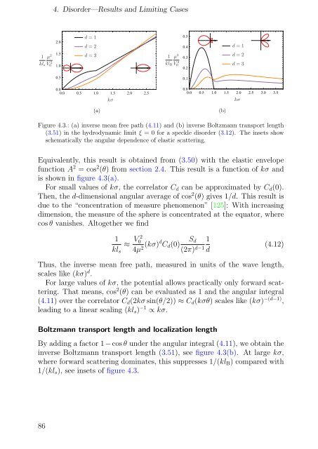
Figure 4.3.: (a) inverse mean free path (4.11) and (b) inverse Boltzmann transport length
(3.51) in the hydrodynamic limit ξ = 0 for a speckle disorder (3.12). The insets show
schematically the angular dependence of elastic scattering.
Equivalently, this result is obtained from (3.50) with the elastic envelope
function A 2 = cos 2 (θ) from section 2.4. This result is a function of kσ and
is shown in figure 4.3(a).
For small values of kσ, the correlator Cd can be approximated by Cd(0).
Then, the d-dimensional angular average of cos 2 (θ) gives 1/d. This result is
due to the “concentration of measure phenomenon” [125]: With increasing
dimension, the measure of the sphere is concentrated at the equator, where
cos θ vanishes. Altogether we find
1
kls
≈
2 V0 4µ 2(kσ)d Cd(0) Sd
(2π) d−1
1
d
(b)
(4.12)
Thus, the inverse mean free path, measured in units of the wave length,
scales like (kσ) d .
For large values of kσ, the potential allows practically only forward scattering.
That means, cos 2 (θ) can be evaluated as 1 and the angular integral
(4.11) over the correlator Cd(2kσ sin(θ/2)) ≈ Cd(kσθ) scales like (kσ) −(d−1) ,
leading to a linear scaling (kls) −1 ∝ kσ.
Boltzmann transport length and localization length
By adding a factor 1−cos θ under the angular integral (4.11), we obtain the
inverse Boltzmann transport length (3.51), see figure 4.3(b). At large kσ,
where forward scattering dominates, this suppresses 1/(klB) compared with
1/(kls), see insets of figure 4.3.
86