Bogoliubov Excitations of Inhomogeneous Bose-Einstein ...

0.8
0.6
0.4
0.2
3. Disorder
Cd(r/σ)
1
1 2 3 4 5 6
(a)
d = 1
d = 2
d = 3
r
σ
Sd
(2π) d (kσ)d Cd(kσ)
1
0.8
0.6
0.4
0.2
0.5 1 1.5 2
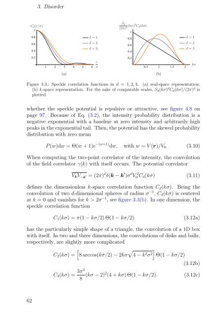
Figure 3.3.: Speckle correlation functions in d = 1, 2, 3. (a) real-space representation.
(b) k-space representation. For the sake of comparable scales, Sd(kσ) d Cd(kσ)/(2π) d is
plotted.
whether the speckle potential is repulsive or attractive, see figure 4.8 on
page 97. Because of Eq. (3.2), the intensity probability distribution is a
negative exponential with a baseline at zero intensity and arbitrarily high
peaks in the exponential tail. Then, the potential has the skewed probability
distribution with zero mean
(b)
d = 1
d = 2
d = 3
P (w)dw = Θ(w + 1)e −(w+1) dw, with w = V (r)/V0. (3.10)
When computing the two-point correlator of the intensity, the convolution
of the field correlator γ(k) with itself occurs. The potential correlator
VkV −k ′ = (2π) d δ(k − k ′ )σ d V 2
0 Cd(kσ) (3.11)
defines the dimensionless k-space correlation function Cd(kσ). Being the
convolution of two d-dimensional spheres of radius σ −1 , Cd(kσ) is centered
at k = 0 and vanishes for k > 2σ −1 , see figure 3.3(b). In one dimension, the
speckle correlation function
C1(kσ) = π(1 − kσ/2) Θ(1 − kσ/2) (3.12a)
has the particularly simple shape of a triangle, the convolution of a 1D box
with itself. In two and three dimensions, the convolutions of disks and balls,
respectively, are slightly more complicated
62
C2(kσ) =
�
8 arccos(kσ/2) − 2kσ � 4 − k2σ2 �
Θ(1 − kσ/2)
kσ
(3.12b)
C3(kσ) = 3π2
8 (kσ − 2)2 (4 + kσ) Θ(1 − kσ/2). (3.12c)