Bogoliubov Excitations of Inhomogeneous Bose-Einstein ...

More documents

Recommendations

Info

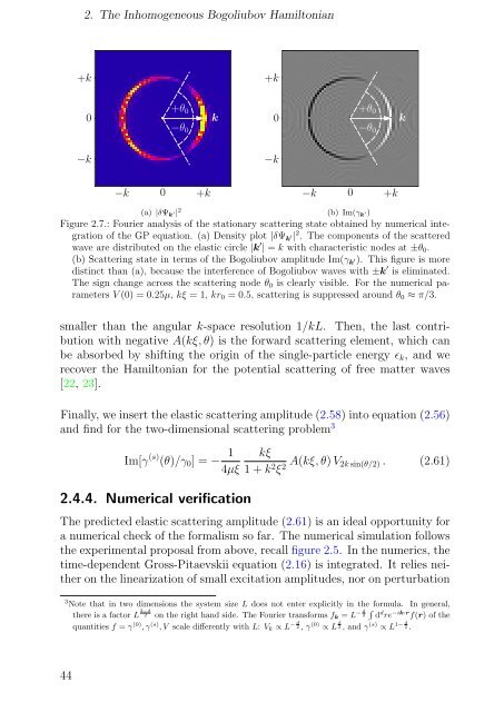
2. The Inhomogeneous Bogoliubov Hamiltonian +k 0 −k +θ0 −θ0 −k 0 +k k −k 0 +k (a) |δΨk ′|2 (b) Im(γk ′) Figure 2.7.: Fourier analysis of the stationary scattering state obtained by numerical integration of the GP equation. (a) Density plot |δΨk ′| 2 . The components of the scattered wave are distributed on the elastic circle |k ′ | = k with characteristic nodes at ±θ0. (b) Scattering state in terms of the Bogoliubov amplitude Im(γk ′). This figure is more distinct than (a), because the interference of Bogoliubov waves with ±k ′ is eliminated. The sign change across the scattering node θ0 is clearly visible. For the numerical parameters V (0) = 0.25µ, kξ = 1, kr0 = 0.5, scattering is suppressed around θ0 ≈ π/3. smaller than the angular k-space resolution 1/kL. Then, the last contribution with negative A(kξ, θ) is the forward scattering element, which can be absorbed by shifting the origin of the single-particle energy ɛk, and we recover the Hamiltonian for the potential scattering of free matter waves [22, 23]. Finally, we insert the elastic scattering amplitude (2.58) into equation (2.56) and find for the two-dimensional scattering problem 3 Im[γ (s) (θ)/γ0] = − 1 4µξ 2.4.4. Numerical verification +k 0 −k +θ0 −θ0 kξ 1 + k 2 ξ 2 A(kξ, θ) V 2k sin(θ/2) . (2.61) The predicted elastic scattering amplitude (2.61) is an ideal opportunity for a numerical check of the formalism so far. The numerical simulation follows the experimental proposal from above, recall figure 2.5. In the numerics, the time-dependent Gross-Pitaevskii equation (2.16) is integrated. It relies neither on the linearization of small excitation amplitudes, nor on perturbation 3 Note that in two dimensions the system size L does not enter explicitly in the formula. In general, 44 there is a factor L 2−d d � 2 − on the right hand side. The Fourier transforms fk = L 2 d −ik·r d re f(r) of the quantities f = γ (0) , γ (s) d − , V scale differently with L: Vk ∝ L 2 , γ (0) ∝ L d d 1− 2 , and γ (s) ∝ L k 2 .
2.4. Single scattering event theory for a weak potential. The trapping potential is neglected, instead, the impurity potential is placed into a finite homogeneous system with periodic boundary conditions. In order to investigate the interesting envelope function (2.59) in the scattering amplitude (2.61), the potential factor V k ′ −k should allow scattering in all directions. That means, the impurity should be pointlike in the sense that its extension r0 should be much smaller than the wave length kr0 ≪ 1. First, the Gross-Pitaevskii ground state is calculated by imaginary-time propagation, using the forth-order Runge-Kutta method [104]. Then a plane-wave Bogoliubov excitation of the unperturbed system is superposed. During the real-time evolution, the wave propagates and is scattered at the impurity. After some time t, the stationary scattering state should be reached in a square with edge length L ≈ c t around the impurity. This part of the system is Fourier transformed and compared to the condensate ground state without the excitation. In the density plot of the scattered wave |δΨ k ′| 2 , figure 2.7(a), one can already observe the node of vanishing scattering amplitude (2.60) very clearly. The data shown in figure 2.7(a) still shows the Gross-Pitaevskii wave function. One can get more insight in terms of Bogoliubov amplitudes γ k ′ = uk ′δΨk ′+vk ′δΨ∗ −k ′, with uk = (ɛk+ɛ0 k )/(2�ɛkɛ0 k ) and vk = (ɛk−ɛ0 k )/(2�ɛkɛ0 k ). The corresponding plot of the imaginary part of the Bogoliubov-transformed amplitude in figure 2.7(b) clearly shows the amplitude sign change across the scattering node. Note that figure 2.7(b) is much clearer than figure 2.7(a), because there Bogoliubov excitations with opposite ±k ′ interfere in the wave function densities |δΨk ′| 2 . One may wonder why the superposition of nodes stemming from opposite wave vectors still gives a density dip as clear as in figure 2.7(a). In fact, in the single-particle case kξ ≫ 1, vk/uk tends to zero such that only the node of one component is observed, whereas for sound waves kξ ≪ 1 both components contribute equally, but now with symmetric nodes at ± π 2 that superpose exactly. This node robustness should facilitate the experimental observation. We extract the scattering amplitude from the data on the elastic scattering circle in figure 2.7(b) and plot it together with the analytical prediction (2.61) as function of the scattering angle θ at various wave vectors kξ, as shown in figure 2.8. The agreement is very good, with residual numerical scatter due to transients and boundary effects. Equation (2.61) and figure 2.8 show that the overall magnitude of scattering peaks at kξ ≈ 1, at the crossing from waves to particles. Physically, this results from two competing scalings in (2.56): • The Bogoliubov scattering amplitude W (k, θ) ∝ ɛ 0 k /ɛk is proportional to k for kξ ≪ 1 and saturates to a constant for kξ ≫ 1. 45
Page 1:
Bogoliubov Excitations of Inhomogen
Page 5: Abstract In this thesis, different
Page 8 and 9: Contents 2.5. Exact diagonalization
Page 10 and 11: Contents Bibliography 141 List of F
Page 13 and 14: 1. Interacting Bose Gases—Complex
Page 15 and 16: 1.2. Disorder 1.2. Disorder Idealiz
Page 17 and 18: 1.4. Cold-atoms—Universal model s
Page 19 and 20: 1.5. Cold atoms—History and key e
Page 21 and 22: 1.5. Cold atoms—History and key e
Page 23 and 24: 1.6. Standing of this work are rest
Page 25: 1.6. Standing of this work The disc
Page 29 and 30: 2. The Inhomogeneous Bogoliubov Ham
Page 31 and 32: 2.1. Bose-Einstein condensation of
Page 33 and 34: 2.1. Bose-Einstein condensation of
Page 35 and 36: 2.2. Interacting BEC and Gross-Pita
Page 41 and 42: n(x) n∞ 1 0.8 0.6 0.4 0.2 0 -3 -2
Page 43 and 44: 2.3. Bogoliubov Excitations and pha
Page 45 and 46: 2.3. Bogoliubov Excitations At high
Page 47 and 48: „ Φq ′ ¯Φ q ′ « V „ Φq
Page 49 and 50: (2) k ′ q k = ξ2 � k ′′2 +
Page 51 and 52: k k ′ 2.4.1. Single scattering se
Page 53 and 54: 2.4. Single scattering event back a
Page 55: k + − w (1) k ′ k (a) 2.4. Sing
Page 59 and 60: T 1 B 2 2.5. Exact diagonalization
Page 61 and 62: 2.5. Exact diagonalization of the B
Page 69 and 70: 3. Disorder In the previous chapter
Page 71 and 72: 3.1.1. Speckle amplitude 3.1. Optic
Page 73 and 74: 3.1. Optical speckle potential In c
Page 75 and 76: 3.2. A suitable basis for the disor
Page 77 and 78: 3.2. A suitable basis for the disor
Page 79 and 80: 3.3. Effective medium and diagramma
Page 85 and 86: 3.4. Deriving physical quantities f
Page 87 and 88: 3.4. Deriving physical quantities f
Page 89 and 90: Fixed particle number 3.4. Deriving
Page 91 and 92: ρµξ d 0.2 0.15 0.1 0.05 1 2 3 4
Page 93 and 94: 4. Disorder—Results and Limiting
Page 95 and 96: 4.1. Hydrodynamic limit I: ξ = 0 t
Page 97 and 98: 4.1. Hydrodynamic limit I: ξ = 0 T
Page 99 and 100: 4.1. Hydrodynamic limit I: ξ = 0 I
Page 101 and 102: ǫk 0.25 0.5 0.75 1 1.25 1.5 1.75 k
Page 103 and 104: gd(κ) v 2 1.75 1.5 1.25 1 0.75 0.5
Page 105 and 106: 4.2. Hydrodynamic limit II: towards
Page 107 and 108:
∆ǫk ǫk �0.1 �0.2 �0.3 �
Page 109 and 110:
1 0.5 0 -0.5 0 20 40 60 80 100 x/σ
Page 111 and 112:
ΛN �0.1 �0.2 �0.3 �0.4 4.3
Page 113 and 114:
nnc(V )−nnc(0) nnc(0) 1.2 1.15 1.
Page 115 and 116:
4.4. Particle regime which coincide
Page 117 and 118:
4.4. Particle regime regime, becaus
Page 119 and 120:
0.02 0.015 0.01 0.005 MSg 0.01 0.1
Page 121 and 122:
5. Conclusions and Outlook (Part I)
Page 123 and 124:
5.3. Theoretical outlook potential.
Page 125:
Part II. Bloch Oscillations 113
Page 128 and 129:
6. Bloch Oscillations and Time-Depe
Page 130 and 131:
Page 132 and 133:
Page 134 and 135:
Page 136 and 137:
Page 138 and 139:
Page 140 and 141:
Page 142 and 143:
Page 144 and 145:
Page 146 and 147:
λTB t/TB 0.15 0.05 70 60 50 40 30
Page 148 and 149:
Page 150 and 151:
A. List of Symbols and Abbreviation
Page 152 and 153:
140 A. List of Symbols and Abbrevia
Page 154 and 155:
Bibliography [11] P. A. Lee and T.
Page 156 and 157:
Bibliography [35] M. Lewenstein, A.
Page 158 and 159:
Bibliography [58] J. Stenger, S. In
Page 160 and 161:
Bibliography [81] V. I. Yukalov and
Page 162 and 163:
Bibliography [108] A. Mostafazadeh,
Page 164 and 165:
Bibliography [131] F. Bloch, Über
Page 167 and 168:
Acknowledgments I thank everybody w
show all

Bogoliubov Excitations of Inhomogeneous Bose-Einstein ...

Create successful ePaper yourself

Delete template?

Save as template?