Bogoliubov Excitations of Inhomogeneous Bose-Einstein ...

More documents

Recommendations

Info

2. The Inhomogeneous Bogoliubov Hamiltonian According to the equations of motion (2.30), this is a coupling between phase and density fluctuations, mediated by particles in the non-uniform condensate Φ. The density coupling has a different dependence on the nonuniform condensate. Indeed, by expressing the non-uniform condensate Φ in terms of the inverse imprint ¯ Φ(r) = Φ 2 0/Φ(r), we can write the density coupling in a form analogous to (2.39) R ′ k k = 1 L d 2 � q ˜r k ′ k q ¯ Φk ′ −q ¯ Φq−k, (2.40) with ˜r k ′ k q = � 2 � q 2 − 2(k ′ − q)·(q − k) + � (k ′ − q) 2 + (k − q) 2� /2 � /m. Both formulae (2.39) and (2.40) are non-perturbative. That means they hold for arbitrary external potentials, if only the condensate wave function Φ and its inverse ¯ Φ are determined correctly. Inhomogeneous Bogoliubov Hamiltonian in the free Bogoliubov basis For the further analysis, it is useful to transform to Bogoliubov quasiparticles ˆγk, such that the free Hamiltonian takes its diagonal form (2.34). We use the Bogoliubov transformation (2.33) of the homogeneous problem. In this basis every mode is still characterized by its momentum k. Only the saddle point (n0)k, from where the fluctuations δˆn = ˆn−n0 are measured, is shifted by the external potential. A detailed discussion about this choice of basis is found in section 3.2. Thus, the couplings are transformed in the following way � Wk ′ k Y k ′ k Y k ′ k W k ′ k � = 1 4 � a −1 k ′ −a −1 k ′ ak ′ ak ′ �� Sk ′ k 0 0 R k ′ k � � a −1 and the Bogoliubov Hamiltonian (2.29) takes the form ˆF [ˆγ, ˆγ † ] = � k ɛkˆγ † kˆγk + 1 2L d 2 � k,k ′ k ak � ˆγ † k ′, � ˆγ ′ −k � W ′ k k Y ′ k k Y ′ k k W ′ k k −a−1 k ak � =: V ′ k k, � � ˆγk ˆγ † −k (2.41) � . (2.42) This Hamiltonian for the inhomogeneous Bogoliubov problem is the central achievement of the whole chapter. The equation of motion for the bosonic Bogoliubov quasiparticles ˆγk reads 34 i� ∂ ∂t ˆγ k ′ = � ˆγ k ′, ˆ F � = ɛk ′ˆγ ′ k + 1 L d 2 � k � W ′ k kˆγk + Y ′ k kˆγ † � −k . (2.43)
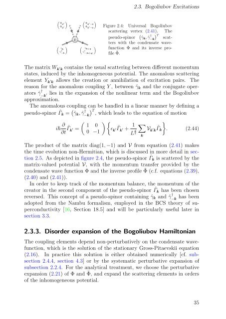
„ Φq ′ ¯Φ q ′ « V „ Φq ′ −q ¯Φ q ′ −q « „ ˆγk ˆγ † « „ ˆγk+q −k ˆγ † « −(k+q) 2.3. Bogoliubov Excitations Figure 2.4: Universal Bogoliubov scattering vertex (2.41). The pseudo-spinor � ˆγk, ˆγ † �T −k scatters with the condensate wavefunction Φ and its inverse profile ¯ Φ. The matrix W k ′ k contains the usual scattering between different momentum states, induced by the inhomogeneous potential. The anomalous scattering element Y k ′ k allows the creation or annihilation of excitation pairs. The reason for the anomalous coupling Y , between ˆγk and the conjugate oper- ators ˆγ † −k ′ lies in the expansion of the nonlinear term and the Bogoliubov approximation. The anomalous coupling can be handled in a linear manner by defining a pseudo-spinor ˆ Γk = � ˆγk, ˆγ † �T −k , which leads to the equation of motion i� ∂ ∂t ˆ � 1 0 Γ ′ k = 0 −1 � � V ′ ˆ k kΓk . (2.44) � � ɛ ′ ˆ k Γk ′ + 1 L d 2 The product of the matrix diag(1, −1) and V from equation (2.41) makes the time evolution non-Hermitian, which is discussed in more detail in section 2.5. As depicted in figure 2.4, the pseudo-spinor ˆ Γk is scattered by the matrix-valued potential V, with the momentum transfer provided by the condensate wave function Φ and the inverse profile ¯ Φ (c.f. equations (2.39), (2.40) and (2.41)). In order to keep track of the momentum balance, the momentum of the creator in the second component of the pseudo-spinor ˆ Γk has been chosen reversed. This concept of a pseudo-spinor containing ˆγk and ˆγ † k −k has been adopted from the Nambu formalism, employed in the BCS theory of superconductivity [16, Section 18.5] and will be particularly useful later in section 3.3. 2.3.3. Disorder expansion of the Bogoliubov Hamiltonian The coupling elements depend non-perturbatively on the condensate wavefunction, which is the solution of the stationary Gross-Pitaevskii equation (2.16). In practice this solution is either obtained numerically [cf. subsection 2.4.4, section 4.3] or by the systematic perturbative expansion of subsection 2.2.4. For the analytical treatment, we choose the perturbative expansion (2.21) of Φ and ¯ Φ, and expand the scattering elements in orders of the inhomogeneous potential. 35
Page 1: Bogoliubov Excitations of Inhomogen
Page 5: Abstract In this thesis, different
Page 8 and 9: Contents 2.5. Exact diagonalization
Page 10 and 11: Contents Bibliography 141 List of F
Page 13 and 14: 1. Interacting Bose Gases—Complex
Page 15 and 16: 1.2. Disorder 1.2. Disorder Idealiz
Page 17 and 18: 1.4. Cold-atoms—Universal model s
Page 19 and 20: 1.5. Cold atoms—History and key e
Page 21 and 22: 1.5. Cold atoms—History and key e
Page 23 and 24: 1.6. Standing of this work are rest
Page 25: 1.6. Standing of this work The disc
Page 29 and 30: 2. The Inhomogeneous Bogoliubov Ham
Page 31 and 32: 2.1. Bose-Einstein condensation of
Page 33 and 34: 2.1. Bose-Einstein condensation of
Page 35 and 36: 2.2. Interacting BEC and Gross-Pita
Page 41 and 42: n(x) n∞ 1 0.8 0.6 0.4 0.2 0 -3 -2
Page 43 and 44: 2.3. Bogoliubov Excitations and pha
Page 45: 2.3. Bogoliubov Excitations At high
Page 49 and 50: (2) k ′ q k = ξ2 � k ′′2 +
Page 51 and 52: k k ′ 2.4.1. Single scattering se
Page 53 and 54: 2.4. Single scattering event back a
Page 55 and 56: k + − w (1) k ′ k (a) 2.4. Sing
Page 57 and 58: 2.4. Single scattering event theory
Page 59 and 60: T 1 B 2 2.5. Exact diagonalization
Page 61 and 62: 2.5. Exact diagonalization of the B
Page 69 and 70: 3. Disorder In the previous chapter
Page 71 and 72: 3.1.1. Speckle amplitude 3.1. Optic
Page 73 and 74: 3.1. Optical speckle potential In c
Page 75 and 76: 3.2. A suitable basis for the disor
Page 77 and 78: 3.2. A suitable basis for the disor
Page 79 and 80: 3.3. Effective medium and diagramma
Page 85 and 86: 3.4. Deriving physical quantities f
Page 87 and 88: 3.4. Deriving physical quantities f
Page 89 and 90: Fixed particle number 3.4. Deriving
Page 91 and 92: ρµξ d 0.2 0.15 0.1 0.05 1 2 3 4
Page 93 and 94: 4. Disorder—Results and Limiting
Page 95 and 96: 4.1. Hydrodynamic limit I: ξ = 0 t
Page 97 and 98:
4.1. Hydrodynamic limit I: ξ = 0 T
Page 99 and 100:
4.1. Hydrodynamic limit I: ξ = 0 I
Page 101 and 102:
ǫk 0.25 0.5 0.75 1 1.25 1.5 1.75 k
Page 103 and 104:
gd(κ) v 2 1.75 1.5 1.25 1 0.75 0.5
Page 105 and 106:
4.2. Hydrodynamic limit II: towards
Page 107 and 108:
∆ǫk ǫk �0.1 �0.2 �0.3 �
Page 109 and 110:
1 0.5 0 -0.5 0 20 40 60 80 100 x/σ
Page 111 and 112:
ΛN �0.1 �0.2 �0.3 �0.4 4.3
Page 113 and 114:
nnc(V )−nnc(0) nnc(0) 1.2 1.15 1.
Page 115 and 116:
4.4. Particle regime which coincide
Page 117 and 118:
4.4. Particle regime regime, becaus
Page 119 and 120:
0.02 0.015 0.01 0.005 MSg 0.01 0.1
Page 121 and 122:
5. Conclusions and Outlook (Part I)
Page 123 and 124:
5.3. Theoretical outlook potential.
Page 125:
Part II. Bloch Oscillations 113
Page 128 and 129:
6. Bloch Oscillations and Time-Depe
Page 130 and 131:
Page 132 and 133:
Page 134 and 135:
Page 136 and 137:
Page 138 and 139:
Page 140 and 141:
Page 142 and 143:
Page 144 and 145:
Page 146 and 147:
λTB t/TB 0.15 0.05 70 60 50 40 30
Page 148 and 149:
Page 150 and 151:
A. List of Symbols and Abbreviation
Page 152 and 153:
140 A. List of Symbols and Abbrevia
Page 154 and 155:
Bibliography [11] P. A. Lee and T.
Page 156 and 157:
Bibliography [35] M. Lewenstein, A.
Page 158 and 159:
Bibliography [58] J. Stenger, S. In
Page 160 and 161:
Bibliography [81] V. I. Yukalov and
Page 162 and 163:
Bibliography [108] A. Mostafazadeh,
Page 164 and 165:
Bibliography [131] F. Bloch, Über
Page 167 and 168:
Acknowledgments I thank everybody w
show all

Bogoliubov Excitations of Inhomogeneous Bose-Einstein ...

Create successful ePaper yourself

Delete template?

Save as template?