Bogoliubov Excitations of Inhomogeneous Bose-Einstein ...

x
xB
1
0.5
0
�0.5
�1
5 10 15 20
t/TB
25 30 35 40
6.5. Collective coordinates
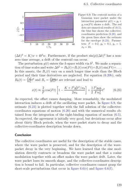
Figure 6.9: The centroid motion of a
Gaussian wave packet under the
interaction parameter g(t) = g0 +
gc cos(F t) shows a drift. The red
dots are numerical results of (6.5),
the blue line shows the collectivecoordinates
prediction (6.20), and
the green lines show the estimate
for the envelope (6.23). Parameters:
F = 0.2, g0 = 0.1, gc = 5,
σ0 = 10.
(∆k) 2 = K/w + 4b 2 w. Furthermore, if the product sin(p)(∆k) 2 has a nonzero
time average, a drift of the centroid can occur.
The perturbation g(t) enters the k-space width via b 2 . We make a separation
of time scales and write ∆b 2 = B0(t)+Bc(t) cos(F t)+Bs(t) sin(F t)+. . . .
In this ansatz, the Bx(t) vary on a much longer time scale than the Bloch
period and their time derivatives are neglected. For equation (6.20b), only
B0(t) = I2 g 2 0
4w 3 0
t 2 and Bs = I2 g0gs
2F w 3 t are relevant and lead to
x(t) ≈ 2
F
cos(F t)
�
1 − K + I2g 2 0t2 �
/w0
2w0
+ 1
2
I2g0gc F w2 t
0
2
(6.23)
As expected, the offset causes damping. More remarkably, the modulated
interaction induces a drift of the oscillating wave packet. In figure 6.9, the
estimate (6.23) is plotted together with the full solution of the collectivecoordinates
equations of motion (6.20) and with the numerical results obtained
from the integration of the tight-binding equation of motion (6.5).
As expected, the agreement is initially very good, but deviations occur after
about thirty Bloch periods, when the wave packet starts to decay and the
collective-coordinates description breaks down.
Conclusion
The collective coordinates are useful for the description of the stable cases,
where the wave packet is preserved, and for the description of the wavepacket
decay in the very beginning. We have learned that the sine modulation
directly contracts or broadens the wave packet and that a cosine
modulation together with an offset makes the wave packet drift. Later, the
wave packet loses its smooth shape, and the collective-coordinates description
is bound to fail. In particular, collective coordinates cannot grasp the
short-scale perturbations that occur in figure 6.6(e) and figure 6.6(f).
129