Bogoliubov Excitations of Inhomogeneous Bose-Einstein ...

√ w
2
1
a.u.
0
-1
10
9.5
(2m) −1 g(t) η ′ (t)
c.c.
0 0.5 1 1.5 2 2.5 3 3.5 4 4.5
6.5. Collective coordinates
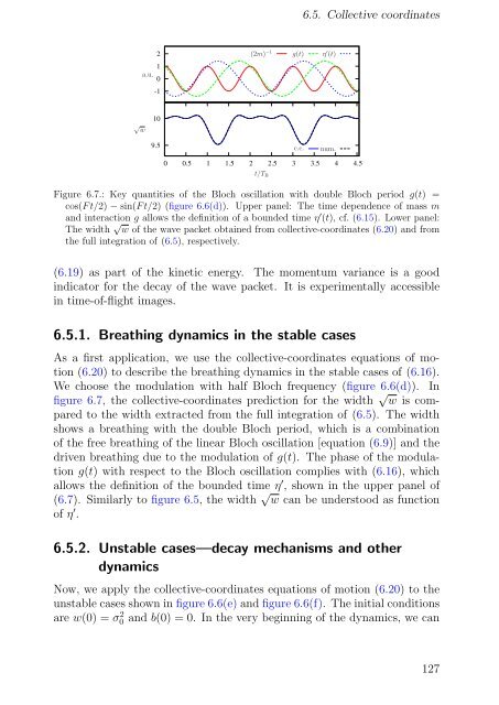
Figure 6.7.: Key quantities of the Bloch oscillation with double Bloch period g(t) =
cos(F t/2) − sin(F t/2) (figure 6.6(d)). Upper panel: The time dependence of mass m
and interaction g allows the definition of a bounded time η ′ (t), cf. (6.15). Lower panel:
The width √ w of the wave packet obtained from collective-coordinates (6.20) and from
the full integration of (6.5), respectively.
(6.19) as part of the kinetic energy. The momentum variance is a good
indicator for the decay of the wave packet. It is experimentally accessible
in time-of-flight images.
t/TB
num.
6.5.1. Breathing dynamics in the stable cases
As a first application, we use the collective-coordinates equations of motion
(6.20) to describe the breathing dynamics in the stable cases of (6.16).
We choose the modulation with half Bloch frequency (figure 6.6(d)). In
figure 6.7, the collective-coordinates prediction for the width √ w is compared
to the width extracted from the full integration of (6.5). The width
shows a breathing with the double Bloch period, which is a combination
of the free breathing of the linear Bloch oscillation [equation (6.9)] and the
driven breathing due to the modulation of g(t). The phase of the modulation
g(t) with respect to the Bloch oscillation complies with (6.16), which
allows the definition of the bounded time η ′ , shown in the upper panel of
(6.7). Similarly to figure 6.5, the width √ w can be understood as function
of η ′ .
6.5.2. Unstable cases—decay mechanisms and other
dynamics
Now, we apply the collective-coordinates equations of motion (6.20) to the
unstable cases shown in figure 6.6(e) and figure 6.6(f). The initial conditions
are w(0) = σ 2 0 and b(0) = 0. In the very beginning of the dynamics, we can
127