Bogoliubov Excitations of Inhomogeneous Bose-Einstein ...

6. Bloch Oscillations and Time-Dependent Interactions
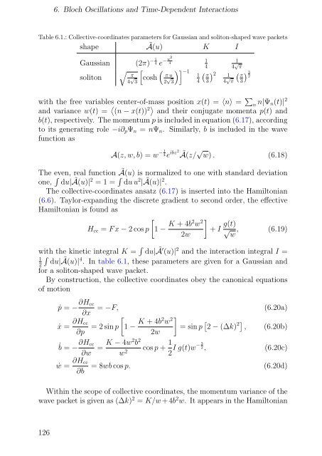
Table 6.1.: Collective-coordinates parameters for Gaussian and soliton-shaped wave packets
shape Ã(u) K I
1 u2
− −
Gaussian (2π) 4 e 4
soliton
� π
4 √ 3
�
cosh
� π u
2 √ 3
�� −1
1
4
1
1
4 4 √ π
� �
π 2 1
3 4 √ �
π
π 3
with the free variables center-of-mass position x(t) = 〈n〉 = �
2
n n|Ψn(t)|
and variance w(t) = � (n − x(t)) 2� and their conjugate momenta p(t) and
b(t), respectively. The momentum p is included in equation (6.17), according
to its generating role −i∂pΨn = nΨn. Similarly, b is included in the wave
function as
1 −
A(z, w, b) = w 4e ibz2Ã(z/ √ w) . (6.18)
The even, real function Ã(u) is normalized to one with standard deviation
one, � du| Ã(u)|2 = 1 = � du u2 | Ã(u)|2 .
The collective-coordinates ansatz (6.17) is inserted into the Hamiltonian
(6.6). Taylor-expanding the discrete gradient to second order, the effective
Hamiltonian is found as
�
Hcc = F x − 2 cos p 1 − K + 4b2w2 �
+ I
2w
g(t)
√ , (6.19)
w
with the kinetic integral K = � du| Ã′ (u)| 2 �
and the interaction integral I =
1
2 du|Ã(u)| 4 . In table 6.1, these parameters are given for a Gaussian and
for a soliton-shaped wave packet.
By construction, the collective coordinates obey the canonical equations
of motion
˙p = − ∂Hcc
∂x
˙x = ∂Hcc
∂p
˙b = − ∂Hcc
∂w = K − 4w2b2 w2 ˙w = ∂Hcc
∂b
= −F, (6.20a)
�
= 2 sin p 1 − K + 4b2w2 �
= sin p
2w
� 2 − (∆k) 2� , (6.20b)
cos p + 1
3
I g(t)w− 2,
2
(6.20c)
= 8wb cos p. (6.20d)
Within the scope of collective coordinates, the momentum variance of the
wave packet is given as (∆k) 2 = K/w +4b 2 w. It appears in the Hamiltonian
126
� 3
2