Bogoliubov Excitations of Inhomogeneous Bose-Einstein ...

1
0.5
0
-0.5
0 20 40 60 80 100
x/σ
(a)
4.3. Numerical study of the speed of sound
1
0.5
0
-0.5
0 20 40 60 80 100
x/σ
(b)
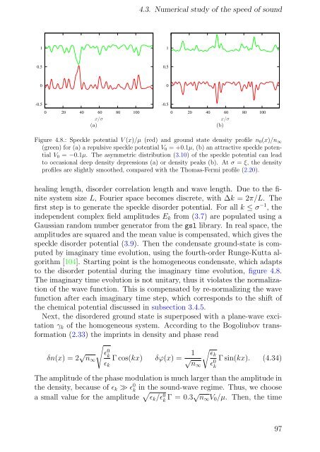
Figure 4.8.: Speckle potential V (x)/µ (red) and ground state density profile n0(x)/n∞
(green) for (a) a repulsive speckle potential V0 = +0.1µ, (b) an attractive speckle potential
V0 = −0.1µ. The asymmetric distribution (3.10) of the speckle potential can lead
to occasional deep density depressions (a) or density peaks (b). At σ = ξ, the density
profiles are slightly smoothed, compared with the Thomas-Fermi profile (2.20).
healing length, disorder correlation length and wave length. Due to the finite
system size L, Fourier space becomes discrete, with ∆k = 2π/L. The
first step is to generate the speckle disorder potential. For all k ≤ σ−1 , the
independent complex field amplitudes Ek from (3.7) are populated using a
Gaussian random number generator from the gsl library. In real space, the
amplitudes are squared and the mean value is compensated, which gives the
speckle disorder potential (3.9). Then the condensate ground-state is computed
by imaginary time evolution, using the fourth-order Runge-Kutta algorithm
[104]. Starting point is the homogeneous condensate, which adapts
to the disorder potential during the imaginary time evolution, figure 4.8.
The imaginary time evolution is not unitary, thus it violates the normalization
of the wave function. This is compensated by re-normalizing the wave
function after each imaginary time step, which corresponds to the shift of
the chemical potential discussed in subsection 3.4.5.
Next, the disordered ground state is superposed with a plane-wave excitation
γk of the homogeneous system. According to the Bogoliubov transformation
(2.33) the imprints in density and phase read
δn(x) = 2 √ n∞
�
ɛ 0 k
ɛk
Γ cos(kx) δϕ(x) = 1
�
ɛk
√
n∞ ɛ0 Γ sin(kx). (4.34)
k
The amplitude of the phase modulation is much larger than the amplitude in
the density, because of ɛk ≫ ɛ0 k in the sound-wave regime. Thus, we choose
a small value for the amplitude � ɛk/ɛ0 k Γ = 0.3√n∞V0/µ. Then, the time
97