Bogoliubov Excitations of Inhomogeneous Bose-Einstein ...

∆ǫk
ǫk
�0.1
�0.2
�0.3
�0.4
µ 2
V 2
0
1 2 3 4
d = 3
5 6
(a)
d = 2
d = 1
4.2. Hydrodynamic limit II: towards δ-disorder
σ
ξ
∆ǫk
ǫk
0.05
�0.05
�0.1
ξ d µ 2
Pd(0)
d = 3
0.2 0.4 0.6 0.8 1
d = 2
d = 1
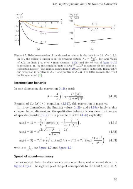
Figure 4.7.: Relative correction of the dispersion relation in the limit k → 0 in d = 1, 2, 3.
In (a), the scaling is chosen as in the previous section, ΛN = . For large values
∆ɛkµ 2
ɛkV 2
0
of σ/ξ, the limit ξ ≪ σ ≪ λ from equation (4.19a) and the left end of figure 4.4(b)
is recovered. In (b) the scaling in units of (σ/ξ) d (V0/µ) 2 is suitable for the limit of δcorrelated
disorder. The limiting results from (4.29) are reached on the left. Remarkably,
the correction is negative in d = 1 and positive in d = 3. The latter recovers the result
by Giorgini et al. [78].
Intermediate behavior
In one dimension the correction (4.28) reads
Λ = − 4
�
dq σ
π
C1(qσ)
(2 + q2ξ2 ) 3.
(b)
σ
ξ
(4.30)
Because of Cd(kσ) ≥ 0 [equations (3.12)], this correction is negative.
In three dimensions, the limiting values (4.29) and (4.19a) imply a sign
change. In two dimensions, the qualitative behavior is less clear. In the case
of speckle disorder (3.12), it is possible to solve (4.28) explicitly:
ΛN(d = 1) = − 3
8 z
�
arccot � z � + 1 z
3 1 + (z) 2
�
, (4.31)
ΛN(d = 2) = z 32z√ 1 + z 2 − 1 − 2z 2
√ 1 + z 2
ΛN(d = 3) = 7z 4 + 5
2 z3 arctan(1/z) − z 4 (6 + 7z 2 ) log
with z = σ
√ 2ξ , see figure 4.7 and figure 4.2.
Speed of sound—summary
� � 2 1 + z
z 2
(4.32)
(4.33)
Let us recapitulate the disorder correction of the speed of sound shown in
figure 4.7(a). The right edge of the plot corresponds to the limit ξ ≪ σ ≪ λ,
95