Satellite Orbit and Ephemeris Determination using Inter Satellite Links
Satellite Orbit and Ephemeris Determination using Inter Satellite Links Satellite Orbit and Ephemeris Determination using Inter Satellite Links
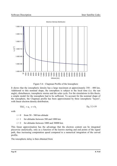
Software DescriptionInter Satellite LinksElectron Density Distribution1.00E+131.00E+121.00E+11n e [m -3 ]1.00E+101.00E+091.00E+081.00E+0750165032504850645080509650112501285014450160501765019250208502245024050256502725028850304503205033650352503685038450Altitude [km]Figure 5-6 Chapman Profile of the IonosphereIt shows that the ionospheric density has a large maximum at approximately 350 – 400 km.Additional to this nominal shape, the ionosphere is subject to the local time (i.e. the sunangle), disturbances, ionospheric storms and the solar cycle. For the simulations in this thesis,a simple model for the ionosphere had to be sufficient. To account for the nominal shape ofthe ionosphere, the Chapman profile has been approximated by three ionospheric "layers",with linear electron density distribution.TEC = a ⋅ r + bEq. 5.3-19iiiwithi = 0 from 50 - 380 km altitudei = 1 for altitudes between 380 and 1000 kmi = 2 for altitudes between 1000 and 30000 kmThis linear approximation has the advantage that the electron content can be integratedpiecewise analytically, only as a function of the known starting and end points of the signalpath, thus increasing computation speed compared to a numerical integration of the curvedprofile.The ionospheric delay is then obtained fromPage 82R. Wolf
Inter Satellite LinksSoftware Description∆IO40.3= ⋅ TEC2fEq. 5.3-20whithTEC Total Electron Content along the signal pathf FrequencyThe error of the model has been assumed to be 50%. This value is added to the observationvariance.5.3.3 Tropospheric ModelA radio signal is also subject to tropospheric refraction, causing a delay in the signal receptiontime, similar to the ionospheric delay, but much less in magnitude. There are severaltropospheric models in use. The one utilised in the simulations is the Saastamionentropospheric model [HWL-94].with∆pTeTr0.002277= ⋅ (p +πcos( - δ)21255π( + 0.05) ⋅ e - tan( - δ))T2atmospheric pressureTemperaturePartial pressure of water vapourEq. 5.3-21δ ElevationIt can be assumed as sufficient to take average values for p and T and e. The residual error hasbeen assumed as 20 % of the result from above equation.5.3.4 Multipath SimulationMultipath is not easy to model, but can be assumed as being a more or less slowly varyingbias. It was simulated using the functionyA⋅sinωt= eEq. 5.3-22which resembles a multipath figure with a slowly varying geometry. All delays and errorshave been added to the measurements as biases.R. Wolf Page 83
- Page 48 and 49: Orbit ComputationInter Satellite Li
- Page 50 and 51: Orbit ComputationInter Satellite Li
- Page 52 and 53: Orbit ComputationInter Satellite Li
- Page 54 and 55: Orbit ComputationInter Satellite Li
- Page 56 and 57: Orbit ComputationInter Satellite Li
- Page 58 and 59: Orbit ComputationInter Satellite Li
- Page 60 and 61: Orbit ComputationInter Satellite Li
- Page 62 and 63: Orbit ComputationInter Satellite Li
- Page 64 and 65: Orbit ComputationInter Satellite Li
- Page 66 and 67: Orbit ComputationInter Satellite Li
- Page 68 and 69: Orbit ComputationInter Satellite Li
- Page 70 and 71: Orbit ComputationInter Satellite Li
- Page 72 and 73: Orbit ComputationInter Satellite Li
- Page 74 and 75: Orbit ComputationInter Satellite Li
- Page 76 and 77: Orbit ComputationInter Satellite Li
- Page 78 and 79: Orbit ComputationInter Satellite Li
- Page 80 and 81: Orbit ComputationInter Satellite Li
- Page 82 and 83: Orbit ComputationInter Satellite Li
- Page 84 and 85: Orbit ComputationInter Satellite Li
- Page 86 and 87: Software DescriptionInter Satellite
- Page 88 and 89: Software DescriptionInter Satellite
- Page 90 and 91: Software DescriptionInter Satellite
- Page 92 and 93: Software DescriptionInter Satellite
- Page 94 and 95: Software DescriptionInter Satellite
- Page 96 and 97: Software DescriptionInter Satellite
- Page 100 and 101: Software DescriptionInter Satellite
- Page 102 and 103: Software DescriptionInter Satellite
- Page 104 and 105: Software DescriptionInter Satellite
- Page 106 and 107: Software DescriptionInter Satellite
- Page 108 and 109: Simulations and ResultsInter Satell
- Page 110 and 111: Simulations and ResultsInter Satell
- Page 112 and 113: Simulations and ResultsInter Satell
- Page 114 and 115: Simulations and ResultsInter Satell
- Page 116 and 117: Simulations and ResultsInter Satell
- Page 118 and 119: Simulations and ResultsInter Satell
- Page 120 and 121: Simulations and ResultsInter Satell
- Page 122 and 123: Simulations and ResultsInter Satell
- Page 124 and 125: Simulations and ResultsInter Satell
- Page 126 and 127: Simulations and ResultsInter Satell
- Page 128 and 129: Simulations and ResultsInter Satell
- Page 130 and 131: Simulations and ResultsInter Satell
- Page 132 and 133: Simulations and ResultsInter Satell
- Page 134 and 135: Simulations and ResultsInter Satell
- Page 136 and 137: Simulations and ResultsInter Satell
- Page 138 and 139: Simulations and ResultsInter Satell
- Page 140 and 141: Simulations and ResultsInter Satell
- Page 142 and 143: Simulations and ResultsInter Satell
- Page 144 and 145: Simulations and ResultsInter Satell
- Page 146 and 147: Simulations and ResultsInter Satell
Software Description<strong>Inter</strong> <strong>Satellite</strong> <strong>Links</strong>Electron Density Distribution1.00E+131.00E+121.00E+11n e [m -3 ]1.00E+101.00E+091.00E+081.00E+0750165032504850645080509650112501285014450160501765019250208502245024050256502725028850304503205033650352503685038450Altitude [km]Figure 5-6 Chapman Profile of the IonosphereIt shows that the ionospheric density has a large maximum at approximately 350 – 400 km.Additional to this nominal shape, the ionosphere is subject to the local time (i.e. the sunangle), disturbances, ionospheric storms <strong>and</strong> the solar cycle. For the simulations in this thesis,a simple model for the ionosphere had to be sufficient. To account for the nominal shape ofthe ionosphere, the Chapman profile has been approximated by three ionospheric "layers",with linear electron density distribution.TEC = a ⋅ r + bEq. 5.3-19iiiwithi = 0 from 50 - 380 km altitudei = 1 for altitudes between 380 <strong>and</strong> 1000 kmi = 2 for altitudes between 1000 <strong>and</strong> 30000 kmThis linear approximation has the advantage that the electron content can be integratedpiecewise analytically, only as a function of the known starting <strong>and</strong> end points of the signalpath, thus increasing computation speed compared to a numerical integration of the curvedprofile.The ionospheric delay is then obtained fromPage 82R. Wolf


