Transactions A.S.M.E.

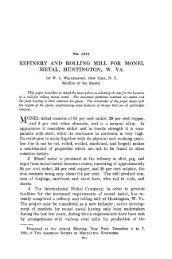
Transactionsof theA.S.M.E.Characteristics of Cloth Filters on Coal Dust-Air M ix t u r e s .......................................................................................................... A. R. Mumjord, A. A. Markson, andT . Ravese 2 7 1Mean Temperature Difference in D e s i g n .......................................................................................................................................R. A. Bowman, A. C. Mueller, and W. M. Nagle 28 3Automatic Control in the Presence of Process Lags . C. E. Mason andG. A. Philbrick 295The Influence of Crystal Size on the Wear Properties of a High-Lead Bearing Metal . .J. R. Connelly 309Calculation of the Elastic Curve of a Helical Compression Spring . . . H. C. Keysor 3 1 9Helix Warping in Helical Compression Springs . . . D. H. Pletta and F. J. Maher 3 2 7Boundary Film InvestigationsHigh-Speed Lightweight TrainsS. J. Needs 3 3 1C. T. Ripley 34 7MAY,VOL. 62, NO. 4

274 TRANSACTIONS OF THE A.S.M.E. MAY, 1940tluced into the cylindrical chamber mentioned with an air injector,making it possible to secure a uniform coating of coal on thecloth, the amount of which was determined by weighing the clothafter each run.The results of these tests are indicated in Fig. 6, which showsthe effect of coal loading on the pressure drop for an air flow of3 cfm free air per sq ft. The curves are plotted for cloths A, Ai,Bi, and B2 and have the same letter designation given in Fig. 5.If, as an example, for cloth A a point at 0.05 lb per sq ft coal-dustloading is taken the pressure drop is 3.4 in. Comparing withFig. 5, a pressure loss of 3.4 in. will pass 102 cfm free air per sqft or 34 times as much air. It will be noted that, in line with thetests of Fig. 5, cloths Bi and B2 will allow more coal accumulationon the cloth for the same pressure-drop and flow conditions thancloths A and Ai. Thus for a 3-in. pressure drop, cloth Ai willallow a coal loading of 0.056 lb per sq ft, whereas cloths Bt and B2will allow 0.078 and 0.083 lb per sq ft, respectively. This, how-than with cloth Ax. No tests were made with cloth B (untreatedcloth) because it had been decided to use flameproofed cloth in theinstallation.Cloth Ai was initially selected for the installation because of itssuperior mechanical properties. It was believed that the heaviercloth would withstand the effects of temperature and beater rodsbetter than the lighter cloths Bi or B2. Flow curves were constructedfor cloth Ai, as in Fig. 7.The design for cloth-filter surface for both mills is contained inTable 3.From the figures given in Table 3, it is evident that the cleaning-periodcycle should be less than 37 min for the 25-ton mill andless than 25 min for the 40-ton mill. It was recognized that thecalculated figures are only approximations because it had beenassumed that the filter cloths were thoroughly clean at the beginningof each cycle. The limited value of the tests, because ofthe number of uncontrolled variables, such as temperature, humidity,dust and sizing, did not justify more accurate determinationof the cleaning cycle. To simplify the control for theseoperations, it was decided to operate both mills with the sameinitial cleaning cycle, a compromise between the two calculatedcleaning cycles.Each filtering unit has four compartments and is so constructedthat one compartment at a time is removed from service forcleaning. It is, of course, important that the cleaning operationoccur only while the compartment is dampered off. The settingadopted is given in Table 4.F i g . 7P r e s s u r e D r o p T h r o u g h C l o t h A i V e r s u s C o a l - D u s tL o a d in gTABLE 4 CYCLE SETTING ADOPTED25-Ton mill 40-Ton millNumber of complete cycles per h r............................ 2 2Time required for 1 cycle, m in.................................. 30 30Total time, unit operating with 100 per cent filteringcapacity, m in.................... . ........................... . 10 10Total time per cycle when unit is operating with75 per cent filtering capacity, m in........................ 20 20Actual shaking time per compartment per cycle,m in...................................................................... .. • • • ^ ^Actual shaking time per compartment per hr, min 6 6Actual shaking time all compartments per cycle,m in........................................................................ 12 12Actual shaking time all compartments per hr, min 24 24N o t e : Time control for the cycle was obtained from a synchronous motorthrough reduction gears driving a shaft onto which were fastened bakelitecams opening and closing contact switches in proper sequence for damperand shaker motor operation. Provision was also made for manual operationof the control limit switches.ever, does not mean that the normal operating pressure of thecloth filters will be less with cloth Bi or B2 than with cloth Ai,but rather that cloths Bi and B2 will retain more coal on theirsurfaces than cloth Ai and that the residual loading, after thecleaning period of cloths Bi and B2, is more than with cloth Ai.The normal operating pressure is approximately the same witheither cloth as borne out by actual operating experience with bothcloths.Observations made during these tests indicate that coal dustpasses through the cloth when it is clean until the pores becomefilled with dust particles to a point when no more coal dust passesthrough. The dust retained on the cloth provides a mat filteringmedium. This effect is more noticeable with cloths Bi and B2TABLE 3 CLOTH-FILTER SURFACE AS DESIGNED25-Ton mill 40-Ton millCoal milled, lb per h r............................................ 50000 100000Coal to cloth filters, lb per h r.............................. 800 1600Vented air, cfm........................................................ 15000 27500Free air cfm per sq ft cloth area (100 per centarea assumed)...................................................... 2.1 2.6Free air cfm per sq ft cloth area (75 per centarea)................................... ................................... 2.8Total cloth area, sq f t ............................................ 7040 *^710Reduced area, 75 per cent of total, sq f t......... 5280 8030Coal-dust loading, lb per M sq ft to give 4 in.normal operating pressure at reduced area... 71 62Total coal on cloth filters, lb ................................ 500 665Shaking interval, m in.....................................................37 25The validity of such testing with respect to the resistance ofdifferent cloths has a good degree of plausibility, since it is possibleto test the cloths under practically identical Reynolds-numberconditions as exist in the full-scale apparatus. These tests indicatethat the effective filter resistance is principally determinedby the filter mat which is formed by the cloth and the so-calledresidual dust loading. To a considerable degree, independenceof filter resistance to the textile specification of the cloth exists,a fact of interest because cloths may be selected principally fortheir mechanical qualities.If it should be found that such tests furnish an approximatebasis for the design, they would assume considerable importance.The authors’ results indicate that this is only roughly true.Since such correlation was not of primary interest at the timeof carrying out the work, necessity for further and more extensivedata is indicated, especially on different materials.The laboratory tests indicate two apparent flow-resistancerules. First, at constant loading of the cloth the draft loss variesdirectly as the flow. This is reasonable enough as the flowthrough the filter itself must be viscous. Second, at constant airflow, the draft loss varies as the 1.5 power of the loading, a statementby no means so obvious and which must be confined to thelimits of the experiments, because it involves several variables

MUMFORD, MARKSON, RAVESE—CLOTH FILTERS ON COAL DUST-AIR MIXTURES 275connected with dust sizings, atmospheric conditions, and othersnot under controlled variation in the experiment.F ie l d T e s t sThe installation of the 25-ton-mill filter was completed in thespring of 1937 and placed in service immediately thereafter.For the first several days, operation of the collector was as expected.Initially some coal dust came through the cloth onto theclean side until a dust mat was formed on the cloth after whichthe air coming through the cloth was perfectly clean. Subsequentoperation of the collector showed that the air resistance keptbuilding up and no amount of shaking would bring it back tonormal while the mill was in service, although the shaking waseffective with the mill shut down. After numerous tests, it wasdecided to change the timing cycle. New cams were ordered, cut,and installed, which permitted more flexibility in the time-controlvariation by resetting the cams on the drive shaft and changingthe motor reduction gears.During the shaking cycle, the sequence of the cleaning operationis as follows:1 Close off compartment to filtering by damper.2 Time prior to shaking called “rest period.”3 Shaking period.4 Time after shaking called “settling period.”Changes were made in the number of cleaning cycles per hourand the rest, shaking, and settling periods.Some of the results of the tests have been plotted in curve formin. and the mill was shut down. In each run the milled coal was21 tons per hr, air flow approximated 14,000 cfm, dry-bulb temperature125 F, and relative humidity 40 per cent. No effect ofthe cycle frequency on the filter back pressure is apparent exceptthat the results with the 3-cycle frequency are worse than withand indicate the rate of pressure build-up. Fig. 8 is a typicalcurve of the initial cycle for 75 per cent filtering area. Duringpart of this cycle 100 per cent filtering area was used. However,so that the test results of the original cycle may be comparedwith subsequent data on cycles which employ 75 per cent filteringarea all of the time, the results were plotted for 75 per centfiltering area. In a period of 2 hr 5 min pressure built up to 4 in.,the normal design pressure, and increased to 51/ i in. in an additional47 min, resulting in a lifting of the explosion vents. After2 hr 45 min of service the time control was changed to manualwith 4 cycles per hr and 60 sec shake, but pressure continuedto build up until the vents were continually open. The millwas shut down after 5 hr 45 min of service because of excessiveback pressure.Figs. 9, 10, and 11 are plots of results of the tests in which thecleaning cycles per hour, rest, shaking, and settling periods werechanged as indicated on the curve sheets. All tests indicate thefilter back pressure rises to 4 in. from 2 to 3Vi hr and, withthe exception of one test (Fig. 10) in which 4 in. is reached inabout IV 2 hr, continued to increase until the vents lifted at 5'Athe 4 or 5 cycle. The duration of the shaking period had no effecton the pressure build-up.Continued checking of the shaker mechanism and damperoperatingmechanism indicated them to be in good working condition.When the damper closed off a compartment to air flow,preparatory to shaking, there was a gradual drop in pressure byvirtue of the fact that flow occurs until the pressures on bothsides of the filter cloth are in balance. If the time allotted forpressure balance is not sufficient or is offset by air leakage around

276 TRANSACTIONS OF THE A.S.M.E. MAY, 1940the damper seal, then shaking of the cloth no m atter what theduration will be ineffective. A checkup of the compartmentpressure, when dampered off, indicated a positive pressure ofapproximately 0.02 to 0.04 in. of water.During the test run plotted in Fig. 11, two of the vent doorswere lifted accidentally while the compartments were damperedoff, thus allowing quick equalization of clean- and dirty-side pressuresand also providing a sufficiently large area for escape of anyinleakage without affecting the pressure balance. The effects werereadily apparent. The filter resistance dropped from 6.10 to4.10 in., after one of the compartment filters had been cleaned,and dropped to 3 in. after the cleaning of the second compartmentfilters. The pressure increased to 4.4 in. as the first then thesecond compartment on which the vent doors had been liftedwere removed from service. The pressure dropped from 4.4 to3.45 in. when both filtering compartments were returned toservice.D e s ig n o f I I e s id u a l -P b e s s u b e R e l e a s e Sy st emWhen the pressure filter system, as previously indicated, wentinto operation the resistance built to very high values. Increasein the individual lines, which may be tapered nozzles, properlydesigned and discharging in the inlet plenum. The over-allsystem resistances including the nozzles should be calculated becausehigh line velocities should be used. The total flow intothe fan under operating conditions is readily figured and leads tothe selection of a fan of proper P-V characteristics. Low velocitiesand flat spots must be avoided as shown in Fig. 12.The power requirements of this fan are a charge against operationamounting to 7 hp for the 7040-sq ft filter and 12 hp for the10,710-sq ft filter.The necessity for some such installation would exist whetherthe filter were under pressure or suction. However, for a suctionfilter, a simple mechanical atmospheric break on the clean sidemight be provided for each compartment.The reasoning indicating the necessity for evacuation is expressedmathematically in the following expression which offersa means for evaluating the time which must elapse before theparticles may be shaken off in the face of a slight residual pressure.If Qtt V, P, are, respectively, the weight of air in the filter, thevolume of the filter, and the absolute filter pressure at any time tand the time derivative isF i g . 12E x h a u s t e b - F a n A b b a n g e m e n t f o b O f e b a t i o n o f D u s tF i l t e bof the number of shaking periods and of the time of shaking wasineffective in eliminating pressure build-up. One theory advancedwas that the residual air pressure in the isolated compartmentheld the coal against the filter in spite of efforts to shake itfree. Tests were run to determine the amount of evacuation necessaryto allow the free discharge of the dust from the cloth.It was found by measurement of air flow that 275 cfm were requiredfor the filters of 410 cu ft free volume, and 400 cfm for thefilters of 590 cu ft free volume. A margin for damper leakage wasalso allowed.After consideration this evacuation was carried out in themanner shown in Fig. 12. A single fan was connected to allcompartments and continuously operated. Its capacity requirementswere based upon the following criteria:The operating suction at the fan inlet is selected so that variationsin flow from operating and nonoperating compartmentsowing to differences in pressure will be swamped out to a desireddegree. This necessitates the introduction of accurate resistancesF i g . 13 V a b i a t i o n o f B a c k P b e s s u b e W i t h T i m e ; . R e s i d u a l -P b e s s u b e R e l e a s e S y s t e mIf the time for decrease of the pressure to 1/i value is observed,the time for the volume rate discharge to change from Vi to F sis given simply enough by the foregoing ratio, assuming that theinlet damper is tight. Theoretically, at least, if the terminalvelocity of the particles were known, the time the filter was tobe out of service before the pressure decreased to the point atwhich the particles would fall off the cloth would be determinate.

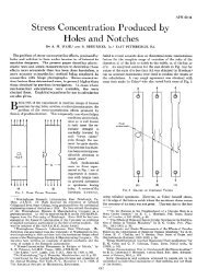
MUMFORD, MARKSON, RAVESE—CLOTH FILTERS ON COAL DUST-AIR MIXTURES 277A consideration of the terminal velocity of fine particles, asdiscussed by Croft,4 leads to the general conclusion that the airvelocities for the particles encountered here must be less thanabout 3.5 in. per sec and may have to be as low as 0.001 in.per sec before shaking can be effective. This consideration indicatesthe necessity for residual-pressure release.The effect of the residual-pressure release mechanism on theback pressure is clearly shown in Fig. 13 which should be comparedwith Figs. 8, 9, 10, and 11.I n s p e c t i o n a n d M a i n t e n a n c eOf particular interest in the operation of the dry dust filtersis the number of man-hours involved in inspection and maintenance.Inspections while the equipment is in service cover thefollowing:1 Lubrication of bearing surfaces of coal-conveyer valves,evacuating fans, and motors.2 Checking housing for leaks from dust side of collector.3 Observation of clean-air discharge for evidence of tom ordefective bags.4 Checking reclaimed-coal lines for free movement of coal.5 Checking operation of main exhauster damper control.6 Checking pressure balance of cloth filter with draft gage.Items 1 to 4 are covered by the regular millhouse operatingcrew and are made a routine m atter along with other duties atsimilar locations about every 2 hr. The inspection is primarilya precautionary measure. Items 5 and 6 are looked after bytest men in the technical department of the company. A monthlyinspection of the damper control is all that is generally necessaryand requires about 3 or 4 hr per month. Item 6 is included for thepurpose of checking the auxiliary-fan operation and is made aboutevery 3 or 4 months in about Vi hr.During the shutdown operation it is advisable to check thefollowing and do general internal cleaning:1 Shaker mechanism.2 Inspect damper gaskets.3 Inspect auxiliary-fan piping.It is good practice to make a general internal inspection of thecollector weekly.Maintenance data on the dust filters are not as complete asthey should be at this time because included in the maintenancefigures are design changes. These changes in design will undoubtedlylower maintenance charges and decrease outage periodsin the future. Figures subsequently cited are for the totaloperating hours given for each filter.The largest single item of maintenance in the dust filters is thefilter bag. Bag life is approximately 2 yr and the bags, withflameproofing applied, cost approximately $1 each. To removeand replace bags requires about 180 man-hr for the 25-tonmill and 275 man-hr for the 40-ton mill, assuming all bags are replaced.Defective bags are located from the clean side of thecollector and are replaced from the dust side of the collector.Since there are 552 bags in the 25-ton-mill installation and 840bags in the 40-ton-mill installation, this replacement is thereforean appreciable item and worthy of investigation.At the present time, tests are under way to confirm a proposeddecrease in shaking frequency and time. One other change hasbeen made which should improve the life of the bags. Formerlythe flow of clean air was downward but now the flow is upwardthrough the top, in order to prevent clean air with high vapor‘ “The Calculation of the Dispersion of Flue Dust and CindersFrom Chimneys,” by H. O. Croft, Trans. A.S.M.E., vol. 57, 1935,paper FSP-57-1, pp. 5-10.content passing from one collector to the other when one of thecollectors is out of service.The next largest item of maintenance is general cleaning andgasket repair. Approximately 400 man-hr have been spent inthis work but it is reasonably certain that this item will virtuallydisappear, because 90 per cent of the time devoted to cleaningwould not have been necessary if the collector were dust-tightinitially. For example, the access doors and coal-hopper casingleaked dust continually while the collectors were in service andrequired constant cleaning and patching, which otherwise wouldnot have been necessary. Dust-tight access doors were made toreplace the initial doors and the hopper casing was welded tomake it dust-tight. Gasket maintenance is a relatively smallitem and has approximated 50 man-hr, which time is spentabout once a year renewing gaskets on explosion vents, accessdoors, and damper frames.Reclaimed coal drive systems have bad approximately 330man-hr maintenance, a considerable portion of which can be consideredas due to the dusty atmosphere, resulting from leakagewhich in turn caused bearing maintenance and maintenance ofthe chain drive. Rotary valves which feed the coal into thescrew conveyer and return coal pipe have had no maintenance.Some trouble had been experienced in the early days with floodingof the conveyer screw, causing plugging of the return coalpipe at the point where it connects to the screw, but this has beenrectified by increasing the angle of inclination of the outlet coalpipe. At the present time the coal drive system runs continuously,but it is planned to try out intermittent operation of thedrive system which, if successful, will decrease maintenance.The shaker mechanism has needed 205 man-hr of maintenancewhich has been due largely to wear of the roll which fits in thecam groove of the rocker mechanism. The roll was worn eggshapedbecause it did not rotate with the cam but slid in the camgroove. Some of the rolls were worn down to the pin in a periodof 6 to 8 months but, when a grease-seal ball bearing was substitutedas a cam follower in place of the hardened steel roll, veryslight uniform wear resulted in a period of 18 months. Therehas been some loosening up and falling out of setscrews fastenedto the rocker shafts which have been replaced with a self-lockingtype of setscrew.Approximately 75 man-hr have been charged to resetting limitswitches. This is not excessive, since it is good practice to checkthe limit switches on the gate-damper motors about once every6 months. The purpose of the check is to insure a good seal ofthe damper against the door frame at all times so that the pressurebalance of the cloth will be proper for effective shaking.The 25-ton mill has been in service 6197 hr and the 40-ton mill5759 hr since the installation of the dry filters. During this timeit is estimated that 4400 tons of coal have been reclaimed by thedust filters. The operation of the filters has been normal and nomajor incidents in their operation have occurred.S a f e t y M e a s u r e sIt is recognized th at coal milling is a process which must becarefully handled to prevent fires during the operation. Protectiveequipment and safe procedures had been employed in themillhouse in line with best practice and this policy was extendedto the dry filters. Numerous tests on filter cloth, both treatedand untreated with flameproofing, indicated the desirability oftreating the cloth, although it was recognized that such treatmentwould increase the flow resistance of the cloth slightly andperhaps affect its life. The effect of the flameproofing was foundto be that of retarding the burning of the cloth and localizing it,although the time required for ignition of the treated and untreatedcloth seemed the same.Long horizontal runs of pipe are objectionable as are low pipe

278 TRANSACTIONS OF TH E A.S.M.E. MAY, 1940velocities. Accordingly in the layout of the pipe lines leadingto the collector, the velocities are maintained at above 3000 fpmand the pipe runs are all practically vertical with the exceptionof the tie-in connection to the collector on the 40-ton mill, whichis approximately 25 ft long. Exposed pipe above the roof is wellinsulated and provided with waterproof covering. In additionthe horizontal run is provided with an inspection and access door.Dry-coal return lines are vertical with minor exceptions, where45-deg bends were necessary. These were provided with cleanoutplugs.It has been mentioned that the dust filters were installed on themillhouse roof. The collector, therefore, had to be well insulatedto prevent condensation. A 4-in. layer of rock wool backed upwith V«-in. transite sheet was provided, the collector itself beinglined with No. 14 gage sheet metal. The temperature dropthrough the collector is therefore small, in the order of 10 F, andthe exit-air temperature is above the dewpoint.Each compartment is provided with an explosion vent in additionto those already existing on the mill proper. Each filteringcompartment has an access door.Published data on the subject of inflammability of coal dustairmixtures are meager with reference to the problem at hand.Two general statements may be made:1 The dust must be present in a cloud of inflammable densityand composition.2 There must be a source of ignition, such as freely burningcoal or an electric spark.These two basic conditions may be discussed in terms of thefactors which determine them. With regard to any distinctionbetween inflammability and explosiveness, investigators of theBureau of Mines6 find, as a practical matter, that it is impossibleto distinguish between them and that it is inadvisable to attem ptsuch distinction.When the coal-air mixture at Kips Bay Station leaves the primarycyclone, the velocities and composition are as given inTable 5.It is also necessary to insure against the hazards of staticelectric discharges. This insurance is largely inherent in the factthat this filter is a mass of metal mesh supporting the cloth,giving almost continuous grounding with a minimum free volumefor the occurrence of intercloud discharges.There is some evidence that high humidities reduce the inflammablecharacter of the mixture, although publications of theBureau of Mines declaim the futility of relying on this. For instance,Rice and Greenwald* unequivocally reject the influenceof humidity in practical work. However, high humidities mayreduce static-electricity hazard considerably.AppendixThree rather complete performance tests on the 40-ton-millcloth-filter installation are given in Table 6. Of particular interestis the power consumption of the cloth filters and the finenessof the reclaimed coal. Power consumption of the cloth-filterinstallation is less than 0.2 kw per ton of milled coal, which isapproximately 1.5 per cent of the total. Fineness of the reclaimedcoal indicates that practically 100 per cent passes through a 325-mesh Tyler screen and also that the density of the reclaimed coalis approximately one half that of the milled coal. It is of interestTABLE 5 VELOCITIES AND COMPOSITION OF COAL-AIRM IXTURE, LEAVING PRIM ARY CYCLONE25-Ton mill 40-Ton millGrains of dust per cu ft of air at 130 F ............... 6.2 6.8Velocity in pipe, ft per m in................................ 3300 3400Dust fineness.......................................................... (100 per cent through 325-mesh Tyler screen)The question of mill drying by flue gases was studied at lengthand abandoned as economically impractical in this instance.The regulation of air flow from the mill to the filters is accomplishedby a high-quality automatic control which throttlesthe mill fan discharge to maintain a constant suction at the millcyclone outlet. This function, the maintenance of constant millair flow, has performed admirably with concurrent advantages inmill operation. Variations in filter pressure are not felt in themill system.On the receiving hoppers of the filter, mechanical rappers wereinstalled and have worked very well. The rotary valves for dischargingthe hoppers are mechanically driven and isolate thehoppers at all times from the receiving screw conveyers.The receiving screw conveyers were the scene of several firesin the early operation due to spontaneous combustion of packedcoal in the barrels. This condition was eliminated by minorchanges. Such precautions are also directed against fire due tospontaneous combustion.6 “ Coal-Dust Explosibility Factors Indicated by ExperimentalMine Investigations, 1911-1929,” by G. S. Rice and H. P. Greenwald,U. S. Bureau of Mines, Washington, D. C., Technical Paper No.464, 1929.F i g . 14R e c l a i m e d - C o a l W e i g h i n g D e v i c eto note that the efficiency of the primary cyclones is better than99 per cent.The tests were made with 4 cleaning cycles per hr on the clothfilters. The duration of each shaking period was approximately20 sec per compartment for each cleaning cycle.The reclaimed-coal weighing device used in these tests is indicatedin Fig. 14. The particular advantage of the installation6 See reference (5); p. 8.

MUMFORD, MARKSON, RAVESE—CLOTH FILTERS ON COAL DUST-AIR MIXTURES 279° Neutral period (all filter compartments filtering).b Cleaning period (one filter compartment closed for shaking).shown is that it permits continuous movement of the coal dust inthe pipe line, because it incorporates a storage hopper in additionto the weighing hopper and also that it is dust-tight which, inthis particular application, is rather important. It is, of course,important if the dust-conveying pipe is under pressure other thanatmospheric that the weighing hopper be vented during theweighing period. For this purpose, a vent valve is provided inthe weighing-hopper cover plate. This particular type of installationhas also been used successfully in weighing flue dust frompulverized-fuel installations. The hoppers are fabricated from®/82-in. plate and all seams are welded.

280 TRANSACTIONS OF THE A.S.M.E. MAY, 1940D iscussionJ. E. F u l w e i l e r .7 It would be interesting to know if anyserious objections to the installation discussed in this paper wereoffered by the engineers of the insurance company covering therisk; also whether the demonstrated safe operation of this completelydry equipment was satisfactory proof that sprays arenot necessary when the other precautions described are taken.In view of the tendency to insist upon sprays in connectionwith explosive industrial dusts, this example may prove of considerablevalue in the art, because some of the dusts involved areof value if kept dry and utterly ruined if wet.The wetting of the dusts also seems to increase rather thanminimize the disposal problem as well as to entail considerabletrouble, due to the freezing of the water in cold weather. Aninstallation of this size and importance, operating dry, is thereforeof considerable interest to the writer.R a l p h A. S h e r m a n . 8 The writer would like to suggest thatsupplementary information covering the proximate analysis andcalorific value of the dust, which is collected in the bag filters,would aid in a comparison of the remainder of the coal collectedin the cyclones.R . F. T h r o n e .® There are upward of 100 installations ofcloth filters in service, handling vents from pulverized-coal equipment.The general experience has been quite satisfactory.Some provisions have been necessary to drain off the staticelectrical charge, and some installations have required specialattention to the slope of the inclined surfaces. Only a few of theinstallations use flue gas as an inert gas, the circulating gas inmost cases being air.Cloth-type filters have the highest reclaim capacity, especiallyin their ability to remove the microscopic sizes under 10ju. Thesesizes represent as high as 80 per cent of the total dust and constitutea major visual nuisance.Precaution must be exercised to maintain the gas humiditybelow 100 per cent, as the resistance through the cloth greatly increasesas it absorbs free moisture, as well as permits the coal dustto cake onto the filter surface, thus increasing the difficulty ofrestoring the filtering medium. The tubular free-hanging typeof cloth filter, can be adequately cleaned in service merely byclosing the outlet-gas damper without in turn closing the inletgasdamper. The agitating mechanism is sufficient to shake thecoal dust from the filter cloth without allowing a time period forequalization of gas pressure on either side. The most effectiveprocedure is to have a reverse flow of the gas through the filtercjoth during the shaking operation, but such reversal, eitherwith the cleaned gas from other sections or with room air, coolsthe gas in the compartment being cleaned, to and below its dewpoint, causing condensation. Cloth filters have proved equallysuccessful under negative pressures as high as 26 in., as well asunder positive pressure. The major disadvantage of negativepressureoperation is the detection of air-inleakage areas.Fire hazard is increased in the employment of cloth filters.This becomes an important factor, especially with the “younger”coals, for which the affinity for oxygen is high. The combustionof filtering cloth with the resulting flame adds a menacing factorto what would otherwise be an easily controllable condition.Flue gas as the circulating medium has not proved satisfactory7 Power and Industrial Engineer, Schmid & Fulweiler, Philadelphia,Pa. Mem. A.S.M.E.9 Supervisor, Fuels Division, Battelle Memorial Institute, Columbus,Ohio. Mem. A.S.M.E.* Secretary-Treasurer, Public Service Company of Colorado,Denver, Colo. Mem. A.S.M.E.in avoiding ignition of coal dust and the resulting loss of filterbags on the “western” coals. Even though a noninflammable filteringcloth material should be developed, considerable questionremains whether with these “younger” coals, the large areaavailable is not a definite hazard.J. C. W i t t . 10 The writer would like to know whether anyinstallations of the type described have been involved in fires?He has had some experience with one all-steel dust-collectorinstallation in which a fire occurred. Much of the equipmentwas rendered worthless by the heat, although nothing was burned.The question therefore arises: What benefit would come from fireproofingthe cloth, in this instance, if a fire should start?A u t h o r s ’ C l o s u r eThe authors believe that the successful operation of the clothfilterinstallation described is in a large measure made possibleby the safety features incorporated in the design and also becauseof the systematic inspection program carried out by theoperating personnel. The insurance carrier, in the case of thisinstallation, interposed no requirements with those on pulverizedcoalinstallations in general.The powdered-coal proximate analyses omitted in the performancetests and requested by Mr. Sherman have been obtained.Average laboratory results of the powdered-coal analyses aretabulated as follows:POWDERED-COAL PROXIM ATE ANALYSESReclaimed coalMilled coal(collected by cloth filter)Moisture, per cent.................................... 1.4 0.8Volatile matter, dry, per cent................ 34.4 33.8Ash, dry, per cent..................................... 7.7 7.4Fixed carbon, dry, per cent.................... 57.9 58.8Sulphur, dry, per cent............................. 1.45 1.10Calorific value, dry basis, Btu per l b . . 14110 14150No appreciable difference in laboratory analyses of the twopowdered-coal samples is evident. Although the primary cycloneefficiency is better than 99 per cent, it is not sufficient to detectdifferences in proximate analysis between milled coal and thevented coal, if such a difference exists. For this installation atleast, the conclusion must be that the proximate analyses of thepowdered coals are the same.Mr. Throne points out that it is necessary to insure againstthe hazards of static electric discharges. This insurance islargely inherent in the collector described. The importance ofmaintaining the temperature of the coal dust conveying air in thecollector above the dew point cannot be overemphasized. Carefulselection of heat-insulating materials has eliminated difficultiesof this kind.Pressure balance of the cloth may be secured by closing eitherthe inlet- or outlet-gas damper. I t is not necessary to close both.In this installation, the inlet dampers were used because it simplifiedconstruction and outlet dampers were not provided becausethey were unnecessary. It has been found by experience thatshaking in a screen-type collector is ineffective if the cloth pressureis unbalanced as little as 0.02 in. of water. Reverse gasflow is unnecessary and is of doubtful value.Mr. Throne states that cloth pressure balance is unnecessarywith the tubular free-hanging-type collector. It is quite unnecessarywith all types if draft loss is no object. I t would beof interest to know the magnitude of the pressure unbalance forthe installation mentioned. It is certain that, if a pressure unbalanceexists at the time of shaking, it is also true that moreeffective shaking is possible if the pressure unbalance is eliminated.Cloth maintenance will be reduced as a result. Needlessly high10 Technical Service Manager, Marquette Cement ManufacturingCompany, Chicago, 111. Mem. A.S.M.E.

MUMFORD, MARKSON, RAVESE—CLOTH FILTERS ON COAL DUST-AIR MIXTURES 281pressure drops should be avoided on large installations becausefan-power requirements will be high and cloth maintenance willbe a very costly item. Although the collector described operatedat a pressure above atmospheric, the system will operate equallysatisfactorily at a pressure below atmospheric. The pressurereleasesystem in the latter case will be rather simple.The authors agree with Mr. W itt that fireproofing the clothdoes not protect the dust-filter equipment after a fire has startedin the collector. As pointed out in the paper, the primary purposeof the cloth flameproofing is that of localizing a fire after ithas started. At this stage, the chief concern of the operator wouldbe to prevent spreading to other parts of the mill system and toadjacent equipment. From this point of view as well as the moralvalue, the slight additional cost of the flameproofing is justified.The authors do not know of any coal-dust cloth-filter installationsof the type of design described in which fires have occurred.There have been fires in the type of collector described with bakelite-dustinstallations and other similar dusts. None of the fireswere directly attributed to the collector but they were carried intoit from other parts of the system.

M ean T e m p e ra tu re D ifference in D esignBy R. A. BOWMAN,1 A. C. M UELLER,2 a n d W. M. NAGLE3In h e a t-tra n sfe r a p p a ra tu s t h e ra te o f h e a t flow fr o m th eh o t to th e co ld flu id is p ro p o rtio n a l t o th e te m p e r a tu r edifference b e tw e en th e tw o . F or d e sig n p u rp o se s, it isnecessary t o b e a b le t o d e te r m in e th e m e a n d ifferen ce intem p eratu re from th e in le t a n d e x it te m p e r a tu r e s. N u ­m erou s in v e stig a to r s have c o n tr ib u te d a n a ly se s o f th e t e m ­p eratu re difference for ex ch a n g ers w ith n e ith e r c o u n te r -nor cocu rren t flow . T h is p ap er co o rd in a tes th e r e su ltso f previou s stu d ie s o n t h e sa m e b a sis t o give a s c o m p letea p ictu re a s p o ssib le o f a ll th e v a rio u s a r r a n g e m e n ts o fsu rface a n d flow . S h e ll-a n d -tu b e exch a n g ers w ith a n yn u m b e r o f p a sses o n sh e ll sid e a n d tu b e sid e are covereda s are th e crossflow exch a n g ers w ith d ifferen t p a ss a r ra n g e­m e n ts a n d w ith m ix ed a n d u n m ix e d flow . T h e sp ecialcases o f tr o m b o n e coolers, p o t coolers, a n d b a tc h p rocesses,n o t p revio u sly p u b lish e d , are a lso tr e a te d in d e ta il.N o m e n c l a t u r eIn this basic equation, the amount of heat transferred per unitof time and surface is shown to equal the product of the over-allheat-transfer coefficient U, and the mean temperature difference,Atm. The value of U may be estimated from correlated over-allcoefficients determined in similar exchangers under similarconditions, or it may be obtained by combination of individualcoefficients. The mean temperature difference Atm is calculatedfrom terminal temperatures, the method of calculation varyingwith the type of exchanger and method of operation.For simple heat exchangers in which there is steady-state operationand countercurrent flow of the hot and cold fluids, integrationof the differential equation, relating the temperatures ofthe two fluids, leads to the well-known log-mean temperature differencefrp ____ f \ ____ rrn ____ a \Atm (countercurrent flow) = —------------——------ —... [2]23 l o g l ° t \— tiTHE following nomenclature is used in the paper:A — area of heating surfaceC = specific heat of shell-side (or hot) fluidc = specific heat of tube-side (or cold) fluide = base of natural logarithmsF = correction factor, dimensionlessM = weight of fluid batchN = number of shell-side passesP = (tj —

284 TRANSACTIONS OF THE A.S.M.E. MAY, 1940paper and, where possible, are expressed in the form of a correctionfactor, F, by which the log mean At for countercurrentflow is multiplied to give the true mean temperature difference.This method of presentation is believed to show most clearly thedegree to which the mean temperature difference of any exchangeris inferior to the log-mean At for countercurrent flow.M u l t ip a s s H e a t E x c h a n g e r sThe widely used shell-and-tube heat exchangers are oftenprovided with baffled heads to route the fluid inside the tubesback and forth from one end of the exchanger to the other.In some cases the shell-side fluid is also caused to travel the lengthof the heat exchanger more than once by means of longitudinalbaffles. Differential equations for a number of such arrangementshave been derived and integrated. In the integration thefollowing assumptions are made:1 The over-all heat-transfer coefficient U is constant throughoutthe heat exchanger.2 The rate of flow of each fluid is constant.3 The specific heat of each fluid is constant.4 There is no condensation of vapor or boiling of liquid inpart of the exchanger.5 Heat losses are negligible.6 There is equal heat-transfer surface in each pass.7 The temperature of the shell-side fluid in any shell-sidepass is uniform over any cross section.The first five assumptions are those employed in the derivationof the ordinary log-mean temperature-difference formula.The sixth is in accord with usual heat-exchanger design practiceand the seventh is essentially true where many transverse bafflesare incorporated in the exchanger.Multipass exchangers with an even number of tube-side passesper shell-side pass were studied by Nagle (l),4 Underwood (2),Bowman (3), and Yendall(15). Their results are summarized asfollows:One Pass Shell Side; Two Passes Tube Side,. The correctionfactor F for multipass heat exchangers, having one shellsideand two tube-side passes, is plotted in Fig. 1 against P andR. The latter are dimensionless ratios, defined as follows:* Numbers in parentheses refer to the Bibliography at the end ofthe paper.The curves of Fig. 1 are based on the integrated equations obtainedby Underwood (2) and by Yendall, rather than on thegraphical integrations of Nagle (1), from which they differ by asmuch as 2 per cent. The integrated equation for A

BOWMAN, MUELLER, NAGLE—MEAN TEM PERATURE DIFFERENCE IN DESIGN 285F i q . 2C o r r e c t io n - F a c t o r P l o tf o r E x c h a n g e r W i t h T w o S h e l lP a s s e s , a n d F o u r , E i g h t , o r A n tM u l t i p l e o f T u b e P a s s e sF i g . 3C o r r e c t io n - F a c t o r P l o tf o r E x c h a n g e r W i t h T h r e eS h e l l P a s s e s , a n d S i x , T w e l v e ,o r A n t M u l t i p l e o f T u b eP a s s e sF i g . 4C o r r e c t io n - F a c t o r P l o tf o r E x c h a n g e r W i t h F o u rS h e l l P a s s e s , a n d E i g h t , S i x ­t e e n , o r A n t M u l t i p l e o f T u b eP a s s e sF i g . 5C o r r e c t i o n - F a c t o r P l o tf o r E x c h a n g e r W i t h S i x S h e l lP a s s e s , a n d T w e l v e , T w e n t t -F o u r , o r A n t M u l t i p l e o f T u b eP a s s e s

286 TRANSACTIONS OF THE A.S.M.E. MAY, 1940F ig. C o r k e c t i o n - F a c t o b P l o t f o b E x c h a n g e r W i t h O n e S h e l l P a s s , a n d T h r e e , S i x , o r A n y M u l t i p l e o f T d b e P a s s e s ;M a j o b i t t o f T u b e P a s s e s i n C o u n t e b c u b b e n t F l o wThree and More Shell-Side Passes. Bowman (3) developed ageneral method for calculating the F factors of three-six, foureight,six-twelve, etc., heat exchangers from the correctionfactors of one-two exchangers. At any given values of F and R,the value of P for an exchanger having N shell-side and 2Ntube-side passes is related to P for a one-two exchanger by theequationOne Pass Shell Side; Six Passes Tube Side. Nagle (1) foundthat the correction factors for one-six exchangers agreed so closelywith those of one-two exchangers operating with the same terminaltemperatures that the curves of Fig. 1 may be used for thiscase.One Pass Shell Side; Infinite Passes Tube Side. It has beenpointed out by Bowman (3) that the correction factor F for amultipass heat exchanger, having one shell-side pass and avery large number of tube-side passes, approaches as a limit thecase of crossflow with both fluids completely mixed. Even inthe limit, however, the value of F is generally only 1 to 2 per centless than that of the one-two exchangers.Two Passes Shell Side; Four Passes Tube Side. The foregoingdiscussion indicates that the correction factors for heat exchangerswith one shell-side pass and two, four, six, and infinitetube-side passes are essentially the same. In many jobs thatreach the designer, however, these types of exchangers areinefficient or entirely inoperative, and an arrangement givinghigher values of F is required. This may be obtained by theuse of two exchangers in series or of a single exchanger havingtwo shell-side passes and four tube-side passes. The correctionfactor F for two-four exchangers piped in the usual manner toapproach countercurrent flow is given graphically in Fig. 2and algebraically by the following rearrangement of Underwood’sequation for two-four heat exchangersThe derivations leading to Fig. 2 and Equation [8] involve theadditional assumptions that there is no leakage of fluid or heatacross the transverse baffle separating the two shell-side passes.For the special case of R — 1, Equation [9] becomes an indeterminatewhich reduces toThe results are given in Figs. 3, 4, and 5, which may also beused with little error for exchangers that are multiples of theone-four or the one-six, rather than the one-two exchanger.From an inspection of Figs. 1 through 5, it may be seen that,for any value of P and R, the correction factor approaches unityas the number of shell-side passes is increased. This is to beexpected, since a multipass exchanger with several shell-sidepasses approaches the ideal countercurrent heat exchanger moreclosely than does one with one shell-side and two or more tubesidepasses.In all the cases mentioned, the ratio of tube-side to shell-sidepasses is an even number, such as 2,4, or 6. However, Fischer (4)has pointed out that there is some improvement in the meantemperature difference if the ratio of tube-side to shell-side passesis an odd number and the exchanger is so connected that thetube-side fluid is flowing counter to the shell-side fluid in overhalf the passes.One Pass Shell Side; Three Passes Tube Side. The correctionfactors F, for one-three heat exchangers and for two-six,three-nine, and four-twelve exchangers have been derived byFischer (4) and presented in the form of tables and charts. Ineach case, the value of F is greater than is found in exchangershaving the same number of shell-side passes but an even numberedratio of tube to shell passes. The improvement in meantemperature difference resulting from the use of three tube-sidepasses per shell-side pass instead of two or four is, however, byno means as great as that resulting from an increase of one in thenumber of shell-side passes.exchanger are given in Fig. 6.Effect of Variation in Heat-Transfer Coefficient.Correction factors for the one-threeThe preced­

BOWMAN, MUELLER, NAGLE—MEAN TEM PERATURE DIFFERENCE IN DESIGN 287ing derivations are based on the assumption that the over-allheat-transfer coefficient U is constant throughout the heat exchanger.For the case of countercurrent flow in which Uvaries linearly with temperature, Colburn (13) has derived thegeneral heat-transfer equationwhere Ui is the value of U at the T { end of the exchanger and Utat the Ti end. This equation has been combined by Sieder andTate (Industrial and Engineering Chemistry, vol. 28,1936, p. 1434)with the correction factor F for use with multipass heat exchang-Until this equation has been tested more extensively its useshould be limited to multipass exchangers having only one shellsidepass.E x a m p l e s A p p l y in g to M u l t ip a s s E x c h a n g e r sThe examples illustrating the variation of the mean temperaturedifference with type of heat exchanger are shown in Table 1.TABLE 1 EXAMPLES ILLUSTRATING VARIATION OF MEANTEM PERATURE D IFFEREN C E W ITH TYPE OF HEATEXCHANGERExample No. 1:Where Ti = 300 F, T% = 200 F, ti = 100 F, ti = 200 F(ft = 1, p = 0.5)Aim,Exchanger F deg FCountercurrent flow................................................................. 1.000 100.0Six-twelve multipass................................................................. 1.000 100.0Two-pass countercurrent crossflow, one fluid mixed.......... 0.970 97.0Horizontal film-type, helical connection.............................. 0.960 96.0Two-four multipass................................................................... 0.958 95.8Horizontal film-type, return-bend connection..................... 0.916 91.5Single-pass crossflow, both fluids unmixed........................... 0.910 91.0One-three m ultipass................................................................. 0.840 84.0Single-pass crossflow, one fluid mixed................................... 0.835 83.5One-two multipass.................................................................... 0.804 80.4One-four multipass.................................................................... 0.798 79.8Single-pass crossflow, both fluids mixed............................... 0.790 79.0Two-pass cocurrent crossflow, one fluid mixed.................... 0.405 40.5Cocurrent flow.......................................................................... 0 0Example No. 2:Where T\ = 300 F, Ti = 200 F, h = 160 F, ti = 260 F(R = 1, P = 0.714)Atm.Exchanger F deg FCountercurrent flow................................................................. ...1.000 40.0Six-twelve m ultipass...................................................................0.970 38.8Horizontal film-type, helical connection..................................0.795 31.8Two-pass countercurrent crossflow, one fluid mixed.............0.745 29.8Single-pass crossflow, both fluids unmixed..............................0.682 27.3Two-four multipass......................................................................0.645 25.8Horizontal film-type, return-bend connection........................0.395 15.8One-three multipass.....................................................................ImpossibleSingle-pass crossflow, one fluid mixed......................................ImpossibleOne-two multipass.......................................................................ImpossibleSingle-pass crossflow, both fluids mixed............................... ...ImpossibleOne-four multipass.............................. ........................................ImpossibleTwo-pass cocurrent crossflow, one fluid mixed.......................ImpossibleCocurrent flow............................................................................ImpossibleIn the first example, all arrangements except that of cocurrentflow can be used. In the second example only countercurrent-flowheat exchangers, or multipass exchangers, which havetwo or more shell-side passes, can possibly give the desiredresults.In the design of multipass heat exchangers, the general rulesof Fischer (4) applying to mean temperature difference should bekept in mind. These are quoted as follows:1 When the number of tube passes per shell pass is even, themean temperature difference is independent of the direction offlow of the shell fluid in each shell pass.2 When the number of tube passes per shell pass is odd, themean temperature difference depends on the direction of flow ofthe shell fluid in each shell pass and is greatest when the counterflowtube passes exceed the parallel-flow tube passes in eachshell pass.3 In multi-shell-pass exchangers the over-all mean temperaturedifference depends on whether the flow of the fluids betweenthe shell passes is counter or parallel flow.4 The equations available for solving the true mean temperaturedifference applying to multipass heat exchangers can bemade general by letting the T values represent the hot-fluid and tvalues represent the cold-fluid terminal temperature.Use of Correction Factors in Design. From the standpoint ofmean temperature difference alone, it is desirable to use the samenumber of shell passes as of tube passes since by so doing truecountercurrent flow can be obtained. However, structural andservicing considerations limit the number of shell passes, twopasses in general being the maximum number for one shell.On the other hand the minimum number of tube passes is set bythe quantity of fluid, the allowable pressure drop, the availablespace, and the costs of construction. Any reduction in thenumber of tube passes below this figure will result in a loweredheat-transfer rate which may overbalance any gain in meantemperature difference.The usual procedure in designing a heat exchanger is, then,- tochoose the number of tube passes on the basis of the foregoingconsiderations and then to select the number of shell passes whichwill give a satisfactory mean temperature difference. If theuse of two passes gives too low a correction factor, the usual practiceis to divide the required surface among two or more shells inseries.Probably the most noticeable feature of the correction curvesis the fact that they all have a very steep gradient for the lowervalues of the correction factor. In other words, a relatively smallchange in temperature conditions will cause a large change of Fand consequently of the mean temperature difference. It alsofollows that a small deviation from the assumed conditions onwhich the curves are based will cause an appreciable error inmean temperature differences derived from this part of the curves.For instance, an exchanger might be expected to work with amean temperature difference of 50 per cent that of a countercurrentexchanger on the basis of the correction-factor curves,whereas, it may actually be an impossible condition, due to thefact that there is leakage of fluid or heat through the longitudinalshell baffle contrary to the assumption of zero leakage.Consequently, the use of correction factors below 0.8 seems tobe questionable from a design standpoint. In those cases wheresuch low correction factors are indicated, one or more additionalshell passes should be used. Also test data, obtained under conditionswhich give low correction factors, should not be acceptedtoo readily for general application.The use of exchangers with three tube passes per shell passgives some improvement in mean temperature difference andthere are applications where this is of value. Unfortunately,the greatest improvement comes at the lower values of correctionfactor where the use of the calculated data for any type of exchangeris none too safe. Furthermore, mechanical and thermaldifficulties may prevent the use of this arrangement in the majorityof cases.When only the inlet temperatures, rates of flow, heat-transferarea, and coefficient are known, the method of Ten Broeck (5)is especially useful. The exit temperatures are easily obtainedfrom his type of plot, eliminating the necessity of trial-and-errorsolution.

288 TRANSACTIONS OF TH E A.S.M.E. MAY, 1940C b o s s f l o w E x c h a n g e r sCrossflow exchangers have the fluids flowing at right angles,therefore, neither the cocurrent nor countercurrent equationsfor mean temperature differences can be applied. The temperatureof the fluid may vary in a direction normal to its flow aswell as with the direction of flow. At the outlet, all infinitesimalsections of the stream may be at different temperatures as eachwas subjected to a different range of temperatures of the otherfluid. The final outlet temperature is obtained by completemixing of all infinitesimal sections. Mixing may take placewithin the exchanger and, if completely mixed, the fluid will havea temperature gradient only in the direction of flow. Therefore,the mean temperature difference is dependent upon whether eitheror both fluids are unmixed or mixed. In any practical crossflowexchanger, the case of unmixed fluids is more nearly approachedthan that of completely mixed fluids. Shell-and-tube exchangerswith many transverse baffles are not crossflow exchangers because,even though the flow is normal to the tubes, the temperaturechange of the shell fluid is negligible for any baffle pass, thetemperature gradient being parallel to the tubes. Conversely,as the number of shell-side passes in crossflow exchange is increased,the more closely will the case of cocurrent or countercurrentflow be approached.Mathematical analysis of the mean temperature difference in asingle-pass crossflow exchanger was initiated by Nusselt (6, 7).Smith (8) finished the analysis of the remaining cases of singlepasscrossflow and extended it to two cases of two-pass crossflowexchangers. While others have presented equations or methodsto determine the mean temperature difference, only Nusselt (7)and Smith (8) have carried out their calculations and presentedtables or graphs from which the mean temperature differencemay easily be computed from the known terminal temperatures.There are several methods of presenting the results of theanalyses of crossflow; each has certain advantages. Smithand Nusselt use a method in which the temperature-differencerelationships depend upon three parameters which are defined asSubstituting these parameters in the log-mean temperaturedifferenceequation for countercurrent flow yieldsThe method adopted for this paper is that of comparison to thelog-mean temperature difference for countercurrent flow, whichrepresents the maximum obtainable difference. This involvesthe use of F, P, and It which can be expressed in terms of thethree parameters by the following relationshipsBy means of these relationships Smith’s data (8) have been transposedinto the curves Figs. 7 to 11. In the present form, theefficiency of the type of exchanger being considered is given by F.It is also easily apparent whether the exchanger will operateunder the given conditions and what penalty is paid in the form ofa poor correction factor F. For performance calculations on aknown exchanger, the method of Ten Broeck (5) is especiallyuseful.The single-pass crossflow exchanger is the only case which hasbeen completely investigated for all types of flow. Only severalof the more important types of flow have been presented for thedouble-pass exchanger and the double-pass trombone exchanger.Mean temperature differences for more than two passes havenot been determined except for the trombone exchangers. Asthe number of passes increases, the log-mean temperature differencefor cocurrent or countercurrent flow will be approached,but no rule can now be given for the number of passes requiredbefore serious errors are introduced by use of these limits.The integrations for mean temperature difference were madeunder the following assumptions:1 The over-all heat-transfer coefficient U is constant throughoutthe heat exchanger.2 The rate of flow of each fluid is constant.3 The specific heat of each fluid is constant throughout theheat exchanger.4 There is no condensation of vapor or boiling of liquid inpart of the exchanger.5 Heat losses are negligible.6 There is equal heat-transfer surface in each pass.7 The fluid is either unmixed or completely mixed normal tothe flow, depending upon the type of flow assumed.

BOWMAN, MUELLER, NAGLE—MEAN TEM PERATURE DIFFERENCE IN DESIGN 289

290 TRANSACTIONS OF TH E A.S.M.E. MAY, 1940Single Pass; Both Fluids Unmixed. Each fluid crosses in aseries of independent infinitesimal streams between which thereis no mixing or heat transfer until the outlet is reached. Sinceeach stream is subjected to a different range of temperatures ofthe other fluid, the streams will have different outlet temperatures,the final outlet temperature being the result of mixing ofall streams. This assumption represents only the limit for anyactual heat exchanger. However, it is nearly approached whenone fluid flows through many tubes and the second fluid, crossingoutside the tubes, is divided into many streams by baffles. Inplate exchangers, mixing is prevented by baffles on each side.This type of crossflow has been frequently investigated.Nusselt’s first solution (6) contained slowly converging seriesand in a later paper (7) a more rapidly converging series wasobtained. Roszak, Veron, and Tripier (9), Binnieand Poole (10),and Liebaut (11) have all presented solutions of varying complexity.Fig. 7 was obtained from values calculated by Nusseltand based on the equationSingle Pass; One Fluid Mixed, Other Unmixed. In this case,one fluid is so completely mixed normal to its flow that there is notemperature gradient. The second fluid is assumed to consist ofindependent streams between which there is no mixing. This isapproached by the first fluid flowing across tubes with no bafflesto prevent mixing and the second fluid flowing through tubes.This type of flow is obtained in a single-pass trombone exchanger.Here, as in subsequent cases where one fluid is mixed, p refers tothe mixed fluid, q to the unmixed. Fig. 8 is based on the graphsof Smith (8) which were calculated from the equationComparison of the graphs shows the correction factors F arelower than in the preceding case. If an exchanger is to be designedwith predetermined terminal temperatures, but the choiceof fluid which is to be mixed is open, a larger correction factor Fis obtained if the fluid with the greater temperature^change ischosen for the mixed fluid. However, the increase in most casesis small.Single Pass; Both Fluids Mixed. The remaining limiting casefor single-pass crossflow is where each fluid is completely mixedso there is no temperature gradient normal to its flow. In Fig. 9the correction factor F, is lower than in either of the two othercases. Here it is possible to get into a region where reversedheat flow may take place, that is, near the outlet the original coldfluid may be hotter than the other fluid. Fig. 9 is based on thegraphs of Smith (8) which were calculated from the equationand error for the intermediate temperatures using the correctionfactors for the corresponding single-pass case. The correctionfactor for each pass is the same. Equation [9] is usefulfor countercurrent flow.Ib Fluid A Mixed, Fluid B Unmixed, Passes Connected inInverted Order. This is exemplified by the trombone cooler withreturn-bend connections.Ic Fluid A Mixed, Fluid B Unmixed, Passes Connected inIdentical Order. This is exemplified by the trombone cooler withhelical connections.Id Fluid A Mixed, Fluid B Unmixed, Except Between Passes.Here it is assumed that the unmixed fluid makes two passesthrough the tubes but is mixed to a uniform temperature betweenthe passes. The second fluid is completely mixed at all timesand flows across the tubes of the second and first tube passes inseries. Fig. 10 was obtained from the graphs by Smith (8)which were determined from the equation for the countercurrentcaseTwo-Pass Crossflow Exchangers. Two identical crossflowexchangers may be connected in series in at least ten differentways, as shown schematically in Table 2. Each of these arrangementscan be operated either co- or countercurrent. Thecases which have been partly or completely solved follow:la Both Fluids Mixed. This case can be solved by trialWhen the present case is changed to cocurrent flow it ispossible to obtain reversed heat flow due to the temperatures ofthe fluids crossing. The correction factors F in Fig. 11 applyto the log-mean temperature difference for countercurrent flow

BOWMAN, MUELLER, NAGLE—MEAN TEM PERATURE DIFFERENCE IN DESIGN 291as this is the basis for all other graphs. Fig. 11 is based on thegraphs of Smith (8) which were calculated from the equationlid Both Fluids Unmixed, One Mixed Between Passes. Thiscase is treated by Schumann (14) for co- and countercurrentflow. The method of analysis developed depends upon calculatingeach pass separately. At the present time, no simple relationshiphas been developed to determine the mean temperaturedifference for both passes from the terminal temperatures.One pass is the same case developed by Nusselt, the other, however,is complicated by an initial temperature distribution enteringthe pass.IV d Fluids A and B Unmixed But Mixed Between Passes.This is treated in the same manner as la.H o r iz o n t a l F il m - T y p e E x c h a n g e r sHorizontal film-type exchangers (also called trombone ortrickle coolers) are simply banks of horizontal pipes, one abovehe other, over which a film of fluid is distributed. These exchangersare frequently used because of their simple and cheapconstruction and the ease of cleaning the outside of the pipe.The equations for any number of passes of horizontal filmtypeexchangers have been derived. The cases solved are forcountercurrent flow and for the return-bend and helical systemsof connecting the passes. The usual assumptions given at thebeginning of this section are made. In addition, it is assumedthat the temperature of the fluid, inside the pipe, T, is uniformthroughout its cross section at any point. It is also assumed thatthe liquor flowing over the banks of pipes is not mixed laterally.The final temperature of the liquor, U, is the result of completemixing of each independent stream, which was at a different temperaturewhen leaving the bottom pipe.Return Bends. Here the fluid in the tube in one pass flows in anopposite direction to the fluid in the pass immediately aboveor below. There is only one bank of pipes formed with this systemof connections. Fig. 12 is based on curves obtained for twopasses from the equationwhere K = 1 •— e~ q^2r.Helical Connection. In this case the pipe may be consideredas an elongated coil forming two banks of pipes. The directionof flow through all pipes in a given bank is the same. Fig. 13is based on curves obtained for two passes from the equationM e a n T e m p e r a t u r e D if f e r e n c e f o r T a n k s in S e r ie s ,H e a t e d o r C o o le d b y C o il sThere are occasional processes where a fluid is heated or cooledin a series of tanks by coils. One fluid overflows from one tankto another, each tank being at a different temperature. Fluidin the coils may be in series countercurrent to the tank fluid oreach coil in a tank may be fed separately. The problem in designor analysis of data arises when only the number of tanksand the terminal temperatures are known. A method has beenderived for such cases. For this case, assumptions are made asfollows:

292 TRANSACTIONS OF THE A.S.M.E. MAY, 19401 Heat-transfer area and coefficient in each tank are the same.2 Each tank is at a constant and uniform temperature.3 Heat transferred is sensible heat.4 Specific heats are constant.5 Temperature and flow of fluids are constant.Tanks in Series; Coils in Series CounterflowLet Ti, T i ,..,T n — temperature of feed to first, second,. . . n tank= temperature of coil liquid leaving the first,second, . . . n tank= temperature of liquid entering n tankFig. 14, the line OC is drawn through point Ti, h with a slope ofR. The line OH is drawn to divide any horizontal segmentGI between OG and the diagonal 01 in such proportion thatG I/H I = . By similar triangles G I/H I = GE/HJ, which latterexpression is by definition. The temperature in any tank isfound by proceeding stepwise from T i and

BOWMAN, MUELLER, NAGLE—MEAN TEM PERATURE DIFFERENCE IN DESIGN 2932 The specific heat of each fluid is constant.3 Only sensible heat is involved, there being no changeof phase or heats of reaction.4 The batch fluid is well agitated and of uniform temperatureT.5 Heat losses are negligible.6 The over-all heat-transfer coefficient U is constant.The general design equation iswhere (T — ta)m is the log-mean difference of the terminal batchtemperatures and the inlet temperature of the medium.Either Equation [32] or [33] may be used depending upon theinformation available. Equation [32] is useful when the temperaturerise of the heating or cooling medium is known at anytime 0 and batch temperature T. With this equation experimentaldata may easily be investigated to determine the variationof the over-all coefficient U. If the over-all coefficient variesas a straight-line function of temperature T, then Colburn (13)has shown that the value of UAtm should be the log mean ofUiAti and U2 Afi. Equation [33] is useful in design because it isnot necessary to know the exit temperature of the flowing fluid.The foregoing equations were derived on the assumption of completemixing of the batch at any time; this,however, is seldom realizedin actual operation. In the other extreme of no mixing theproblem is that of unsteady-state conduction. Methods of determiningmean temperature for various degrees of mixing havenot been developed.A c k n o w l e d g m e n tThe authors are grateful for permission to include the previouslyunpublished results of A. P. Colburn for the batch heatingprocess, of T. B. Drew for horizontal film-type exchangers andtanks in series, and of E. F. Yendall on the one-two and one-fourheat exchangers.BIBLIOGRAPHY1 “ Mean Temperature Differences in Multipass Heat Exchangers,”by W. M. Nagle, Industrial and Engineering Chemistry,vol. 25, 1933, pp. 604-609.2 ‘‘The Calculation of the Mean Temperature Difference inMultipass Heat Exchangers,” by A. J. V. Underwood, Journal,Institution of Petroleum Technologists, vol. 20, 1934, pp. 145-158.“Graphical Computation of Logarithmic-Mean Temperature Difference,”by A. J. V. Underwood, Industrial Chemist, vol. 9, 1933, pp.167-170.3 “Mean Temperature Difference Correction in Multipass Exchangers,”by R. A. Bowman, Industrial and Engineering Chemistry,vol. 28, 1936, pp. 541-544.4 “ Mean Temperature Difference Correction in MultipassExchangers,” by F. K. Fischer, Industrial and Engineering Chemistry,vol. 30, 1938, pp. 377-383.5 “ Multipass Exchanger Calculations,” by H. Ten Broeck,Industrial and Engineering Chemistry, vol. 30, 1938, pp. 1041-1042.6 “ Der Warmeiibergang im Kreuzstrom,” by W. Nusselt, ZeitschriftdesVereines deutscher Ingenieur, vol. 55, 1911, pp. 2021-2024.7 “ Eine neue Formel fur den Warmedurchgang im Kreuzstrom,”by W. Nusselt, Technische Mechanik und Thermodynamik, vol. 1,1930,pp. 417-422.8 “ Mean Temperature Difference in Cross Flow,” by D. M.Smith, Engineering, vol. 138, 1934, pp. 479-481, 606-607.9 “ Nouvelles Etudes sur la Chaleur,” by Ch. Roszak and M.V6ron, Dunod, Paris, 1929, pp. 258-267, 731-750.10 “Theory of the Single-Pass Cross-Flow Heat Interchanger,”by A. M. Binnie and E. G. C. Poole, Proceedings, Cambridge PhilosophicalSociety, vol. 33, 1937, pp. 403-411.11 “Note sur les Exchangeurs h Circulation Croisfee,” by AndreLiebaut, Chaleur et Industrie, vol. 16, 1935, pp. 286-290.12 “ Heat Transfer in a Horizontal Coil Vat Pasteurizer,” byR. L. Perry. Published by T h e A m e r i c a n S o c i e t y o f M e c h a n i c a lE n g i n e e r s in “Heat Transfer,” 1935, pp. 61-68.13 “ Mean Temperature Difference and Heat Transfer Coefficientin Liquid Heat Exchangers,” by A. P. Colburn, Industrial and E n­gineering Chemistry, vol. 25, 1933, pp. 873-877.14 “The Calculation of Heat Transfer in Cross-Flow Exchangers,”by E . A . Schumann, Jr., contributed by the A.S.M.E. HeatTransfer Professional Group and presented at the Annual Meeting,Philadelphia, Pa., December 4-8, 1939, of T h e A m e r i c a n S o c i e t yo f M e c h a n i c a l E n g i n e e r s .15 Private communication.D iscussionE. A. S c h u m a n n , J r .6 The writer is well aware of the enormouslabor expended in the preparation of the various correction-factorplots given in this paper and feels that the authors are to bethanked for their contribution to heat-transfer-design data.A comment seems appropriate on the significance of the dimensionlesscorrection factor F in studies of the relative merits ofcounterflow and unmixed crossflow heat exchangers. It is readilyseen that the correction factor represents a ratio of meantemperature differences. .and for identical rates of heat absorption in both types of exchanger,it is apparent that the extent of crossflow heating surfaceneed not be greater than that in the counterflow exchanger, as issometimes supposed.On the contrary, designs which can be adapted to high massflowrates of the shell-side fluid (tubular-type unmixed crossflowexchanger) commensurate with economical pressure drop maybe made to operate with higher shell-side fluid conductances thancould be obtained in a counterflow installation.Finally, any correction factor based on the authors’ argu-6 Engineer, Construction Department, The Detroit Edison Company,Detroit, Mich. Jun. A.S.M.E.

294 TRANSACTIONS OF THE A.S.M.E. MAY, 1940ment P, and fluid ratio R, is only as reliable as the assumptionmade regarding the strictness with which the expected or actualflow directions adhere to the ideal crossflow.A u t h o r s ’ C l o s u r eThe intent of this paper is to present a simplified method fordetermining the true mean temperature difference for varioustypes of flows encountered in heat exchangers from the log-meantemperature difference by applying a correction factor. The correctionfactor F should not be interpreted as indicating the relativemerits of countercurrent exchangers with other flow-typeexchangers as this would hold only under the special conditionsof identical flow rates, temperatures, and heat-transfer coefficients.While it may be possible by using an exchanger other thana countercurrent type to increase the over-all heat-transfercoefficient more than the lowering of the true mean temperaturedifference, there are, however, some types of exchangers forwhich certain temperature conditions cannot be met irrespectiveof the value of the heat-transfer coefficient; this is shown inexample 2 of Table 1. No method of calculating the true meantemperature difference for the crossflow case has been developedfor cases where the flow is not either completely mixed or unmixed;this was specified in the assumptions on which theequations are based.

A utom atic C o n tro l in the Presence ofProcess LagsB y C. E. MASON,1FOXBORO, MASS., a n d G. A. PHILBRICK,2 FOXBORO, MASS.In th is pap er, th e m e th o d s o f " Q u a n tita tiv e A n a ly sis o fP rocess L a g s” d evelop ed in a previou s p a p er3 are ex ten d edto in c lu d e a u to m a tic c o n tr o l. C arryin g o n t h e id ea o fr ep rese n ta tio n b y liq u id -le v e l s y s te m s , a sp ecific sy s te m isp o stu la te d a s a m o d e l for a ty p ic a l in d u str ia l p rocessw h ic h m a y or m a y n o t be th e r m a l. C o n tin u in g th e q u a n ­tita tiv e a p p ro a ch , th e m a th e m a tic a l m a c h in e ry is d e m o n ­str a ted b y w h ic h th e o p eratio n o f c o n tr o l o n p rocessesm a y b e in v e stig a te d . A se lected su c c e ssio n o f c o n tr o ller s,ch a ra cterized b y th e la w s o f con tr o l w h ic h govern th e m ,are consid ered in c o n n e c tio n w ith th e ir p erfo rm a n ce o nth e m o d el sy ste m . A lth o u g h n o a tte m p t h a s b e e n m a d eto fo r m u la te ru les govern in g th e proper a p p lic a tio n o fth e variou s ty p e s o f c o n tr o ller s consid ered or g o v ern in gth e a d ju stm e n t o f a n y o f th e se in d iv id u a l ty p e s, th ea u th o rs consid er th a t a n a ly se s o f t h is so rt m a y w ell servea s a g u id e to p ra ctica l th e o r e m s in a te c h n o lo g y o f a u t o ­m a tic con trol.THE quantitative behavior of certain resistance-capacitysystems was discussed in a former paper3 presentedbefore this Society. These systems exhibited characteristicssimilar to those of industrial processes in which control-resistinglags are found, and were thus proposed as convenientmodels for such processes. To bear out the impliedanalogy, the models themselves, considered as liquid-level systems,were developed side by side with equivalent thermal systems.In this way it was found possible to give definite analyticform to the all-important dynamic properties of equipment towhich the application of automatic control is contemplated,and to justify a professed effort to fill the gap in a literatureotherwise primarily concerned with the properties of the controlsthemselves.Having already dealt with the inherent attributes of a fewsuch model systems, the authors will show in the present paper,how the treatment may be extended to cover their behaviorunder automatic control. The procedure will be to choose aspecific model process to which to apply a succession of types ofcontrols (assumed to be pneumatically operated), the modelbeing one which is representative of a typically difficult prototypesystem, involving a combination of capacity and transfer lags.For concreteness, this prototype system may be considered as athermal process, although it could equally well involve hydraulic,pneumatic, or electrical phenomena, either singly or in combination.Although the alleged purpose of an automatic-control installationis that of holding constant a certain process variable,this is in reality only accomplished by a series of recoveries from1 Director of Control Research, The Foxboro Company.2 Research Engineer, The Foxboro Company.3 “Quantitative Analysis of Process Lags,” by C. E. Mason, Trans.A.S.M.E., vol. 60, May, 1938, pp. 327-334.Contributed by the Committee on Industrial Instruments andRegulations of the Process Industries Division, and presented atthe Annual Meeting, Philadelphia, Pa., December 4-8, 1939, of T h eA m e r i c a n S o c i e t y o f M e c h a n i c a l E n g i n e e r s .N o t e : Statements and opinions advanced in papers are to beunderstood as individual expressions of their authors, and not those ofthe Society.threatening unbalances, the continuity of which constitutesthe record of control. In practice, the disturbances are normallygradual to some degree. It is this fact which makespossible the apparent elimination of the effects of upsetting influences.Since it is obviously impractical to draw conclusions as to theover-all (transient) characteristics of the combined systemthrough the application of any series of influences, it is desirableto select an isolated, suddenly applied, disturbing influence.The results of such a disturbance must involve the completetransient characteristics of the process and controller in combination.The model system selected as representative is shown in Fig. 1.The capacity and resistance elements of which it is constructedare the same sort as previously described.3 Tat Tb, and T c areF i g . 1H y d r a u l ic M o d e l o f a T y p i c a l C o n t i n u o u s P r o c e s slevels (potentials) in the three tanks, the equivalent areas4 (capacities)of which are A a, A b, and A c. These areas are interconnectedthrough the restrictions (resistances) Ra, Rb, and Rc.The flows Qa, Qb, Qc, Q„ and Q„ are disposed as shown.The level Ta in A a is intended to be the controlled variable,while the supply flow Q, is to be given the role of manipulatedvariable by means of which the control of Ta is accomplished.The auxiliary-supply flow Q„ provides a means for altering theload condition, for on the value of this flow depends the value ofTABLE 1Q uantity..........Potential (T) ..Time (

296 TRANSACTIONS OF THE A.S.M.E. MAY, 1940be chosen. Table 1 summarizes these units both for the hydraulicmodel and for the corresponding thermal process.Since the model shown in Fig. 1 is similar in form to that givenas case VI (Fig. 11) in the former paper,3 differing therefromonly in the inclusion of the cascaded capacity A c, it will be appropriateto assign the same numerical values to the constantsof the system, in so far as this is possible (Table 2). The unitsto be assumed for these system constants are as given in Table 1,whether for the hydraulic model or for the thermal prototype.TABLE 2NUM ERICAL VALUES OF SYSTEM CONSTANTSAs pointed out, the original process, of which the hydraulicsystem of Fig. 1 is to be considered a model, might have any oneof a variety of forms. Its nature has been taken arbitrarily asthermal. It might, for example, be thought of as a process identicalwith the two-capacity thermal system shown in Fig. 4 of theprevious paper,3 but with the modification that the electric heatingagency is indirectly manipulated by means of an operationinvolving simple capacity lag, such as exists with a large airmotor setting a current regulator.5 In any event, for presentpurposes it may be assumed that the model has been faithfullyconstructed, and thus the hydraulic system as such may be dealtwith directly. Incidentally, the possibility should not be overlookedthat the original, or prototype, system might be of thesame nature as the model, as for instance a large-scale industrialliquid-level process having transfer lag.Before proceeding to the application of automatic controls,let us briefly discuss the properties of the specific hydraulic system(or analog) from the point of view of the former paper.3Since this is a three-capacity system, the differential equationdescribing the dynamic relation between the significant variables(T„, Q„ and Q„) will be of the third order. The derivationof this equation will not be given in its entirety since it followsstraightforwardly from the methods of the previous paper.The fundamental hydraulic equations areUpon insertion of the numerical values given in Table 24 7 7 " + 18.5 2 7 + 10.25 7 7 + Ta =0.125 (Q. + Q „)„.. [4]in which, by way of recapitulation,Ta = controlled variableQ, = manipulated variableQ0 = auxiliary supply flowThe supply flow Q, is to be operated on by the controlling apparatusin its effort to maintain Ta at a constant value. Theauxiliary flow Q0 will suddenly be changed from one value to anotherunder otherwise steady conditions to provide a disturbanceto the controlled system at an arbitrarily initial instant (t — 0).As in the former paper, let the desired or normal value (To)normof Ta be(2^)norm= 80 (in. or deg)In the thermal counterpart of Fig. 4,3the auxiliary flow Q0 wasthe flow of heat energy—above 0 F—contained in the mechanicalflow of 8 lb per min of water. Assuming again that initially theinlet-water temperature is 60 F, then the disturbance can consistof a sudden decrease in this temperature from 60 F to 40 F.Thus, for the thermal system, the flow Q0 had been initially8 X 60 = 480 Btu/min, while the altered value of Q„ is 8 X 40 =320 Btu/min. Hence for either system(t < 0) Q0 = 480 (lb per min or Btu per min)(< >0) Q„ = 320 (lb per min or Btu per min)Allow the range in which the variable Q, may be changed bythe controls to be given by(Qj)min = Qb = (Qa)maxwhere (Q,)min = 0 (lb per min or Btu per min)(Q,)max = 640 (lb per min or Btu per min)If the controlled variable Ta is to be at its desired value(2 7 norm in the balanced or undisturbed preinitial state, then,since the value of the auxiliary flow Q„ is already determinedfor that epoch, it will be seen from the steady-state version (allderivatives equal zero) of Equation [3] (or Equation [4]) thatthe initial balanced value of Q, must be(Q,)lnlt = [(27n„rm//U — (QJinit = (80/0.125) — 480 = 160Our system is thus prepared for the application of the controllingapparatus which will now be considered.which is the complete process equation for the system of Fig. 1.In the present investigation, the auxiliary flow Q0 will be keptalways at steady values except when suddenly changed from onesteady value to another in simulation of an instantaneous upset;thus for the time intervals consideredQo' = Qo" = 0and the process equation becomes____ {A,)Ta' ” + (A,)Ta” + M ,)2Y + Ta = Ra(Q. + Q „ )... ■[3]5 In this manner, the so-called "valving” lags may be includedas parts of the process rather than as parts of the controls.A p p l ic a t io n o p C o n t r o l A p p a r a t u sThe complete or interconnected control circuit, comprisingboth controlled process and controller, is symbolically shown inFig. 2, in which the process is characterized by the group of itsinherent system constants, and where the other various componentsof the controlled system are shown in their functionalrelationship to one another.Fig. 3 gives a somewhat more realistic picture of the combinedsystem. In Fig. 1 the elements of the process under controlare shown in greater detail.The manipulated supply flow Q, is assumed to be under successfulcontrol by means of a flow controller, in which instrumentthe balanced value of flow, or the flow control point, may be setby the operating means (the pneumatic operating pressure) of thelevel controller, which is the direct analog of a temperature controllerin the thermal counterpart. This instrument contains themeasuring means and the control mechanism, while the flow controlleracts as a positive controlling means. These assumptionswill be followed for all types of control mechanism considered.

MASON, PHILBRICK—AUTOMATIC CONTROL IN THE PRESENCE OF PROCESS LAGS 297Suppose for simplicity that, as the operating air pressure P,Fig. 3, of the control mechanism varies from zero to its maximumvalue, namely, the supply pressure P„ the resulting supply flowQ, maintained by the flow controller varies proportionatelyfrom zero to its maximum value (Q,)m»x. Thus- = [5]P. ( Q ,W ......................................With the operating means of the control mechanism thus directlylinked to the manipulated flow, the equation of the controlmechanism may be expressed as a functional relationship betweenthe controlled variable Ta and the manipulated variableQ„ or asQ, = Fc{Ta) = “controller function” of Ta.............[6]This corresponds to the form of the process equation which maybe writtenTa = Fp(Q,) = “process function” of Q,............. [7]Equations [6] and [7] are of course symbolic since the functionsare in general differential expressions and involve time. TheyF i g . 2F i g . 3D ia g r a m m a t ic C o n t r o l C i r c u i tC o m p l e t e C o n t r o l l e d S y s t e mserve, however, to illustrate the reversal of cause and effect inpassing from process to controller or from controller to process.In tabular form:CauseProcess................... Manipulated variableController..............Controlled variableEffectControlled variableManipulated variableIn the “philosophy” of control, this concept may be consideredbasic.The exact nature of the functional relation Equation [6] willdepend upon the particular type of controller under consideration.The functional relation Equation [7] for the process isprovided in the present case by Equation [3] (and/or [4]). Forpurposes of comparison, not only among the general controllertypes but between different conditions of adjustment for anyone type of controller, the same initial conditions and also thesame manner and magnitude of upset will be assumed throughout.Before taking up the controllers in order, it will be informativeto determine the effect on the controlled variable T„ of the disturbanceto be employed when this disturbance acts on thesystem in equilibrium and with the controls assumed inoperative.The resulting deviation of Ta will be a standard by which to ascertainthe actual amount of correction brought about by the actionof the controllers when operative on the process. Thus, it will beassumed that the foregoing initial conditions are in effect on theprocess and that, at t = 0, the chosen disturbance is inflicted.Since no controller is acting, the supply flow Q, will remain constantat its initial value, while the auxiliary flow Q0 will have itsnew balanced value. Thus from the initial conditions and fromthe process Equation [4]4 Ta + 18.5 T ’ + 10.25 T J + Ta = 0.125 (160 + 320)or(Ta — 6 0 )"' + 4.625 (Ta — 60)" + 2.5625 (Ta — 60)' + 0.25(Ta — 60) = 0 ....................................[8]The solution of Equation [8] to find the variation of Ta as a functionof time is a procedure similar to those described in the previouspaper.8 It involves the roots of the auxiliary algebraicequation.k8 + 4.625 fc2 + 2.5625 k + 0.25 = 0 ....................... [9]and the initial values of the first and second derivatives of T„(rate of change and acceleration immediately following the disturbance).The roots of Equation [9] are all real and negative and may befound by any desired method, although in general for speedand precision Graeffe’s method6 is recommended for any linearalgebraic equation of higher degree than the second. As a m atterof fact Equation [9] is directly factorable in this case (due to thecascaded nature of the analog process) and may be writtenThe roots are thus(k1 -(- 0.625 k + 0.0625) (k + 4) = 0 ................[9a]ka = —0.125 kb = —0.5 k0 = —4 ......... [10]The initial values of the first two derivatives of T a may bedetermined, through the use of Equations [1], from the change inQ0 constituting the disturbance. Since the initial value of thethird derivative of Ta will also be necessary in later examplesand may conveniently be found in conjunction with the othertwo derivatives, all three have been found for the assumed upsetand are listed as follows:(Ta')„ = —5 (in. per min or deg per min ) )(Ta) = +1.875 (in. per min2 or deg per min1) > ..[11](Ta" ')0 = —0.859375 (in. per min8 or deg per min8) JReference to Appendix I7 shows the solution in this case to beof the formT q— Tp = 7’„ — 60 = Caeka‘ + Cbek>‘ + Ccek‘‘........[12]8 “Mathematics of Modern Engineering,” by R. E. Doherty andE. G. Keller, John Wiley & Sons, Inc., New York, vol. 1, 1 9 3 6 , pp.9 8 -1 3 0 .7 The Appendixes referred to throughout the paper form a mathematicalsupplement which does not appear in this publication. Alimited number of copies of this supplement are available, however,and may be obtained from the authors on request.

298 TRANSACTIONS OF TH E A.S.M.E. MAY, 1940where the k’s are the roots given and the C’s are integration constantsinvolving both the roots and the initial values of thederivatives in a manner shown in Appendix l.7 Inserting thenumerical values there resultsTa = 60 + 13.33 e~° l2U + 6.67 e-°-6‘ + 0.00 e-*‘The integration constant Cc is reduced automatically to zerofor the case chosen, since the system is essentially two-capacitywith respect to changes in Q„ alone, Qc Fig. 1 remaining constantalong with Q, for the period considered. Thus for the effect ofthe disturbance on Ta in the absence of controlTg = 60 + 13.33 e-°-126' + 6.67 e-»■«............... [13]Thus when* = 0 Ta = (Ta)„ — 80 (in. or deg) |and when t co Ta —*■(T„) co = 60 (in. or deg) /The behavior of Ta following t = 0 is shown in Fig. 4.An evenbriefly,in connection with the system under consideration, asQ, = (QJmax = 640 for Ta < ( r a)norm = 80 ] [15]Qs ~ (Qt)min— 0 for Ta > (T,a)norm— 80 JSince in operation, the value of Q, is constant except for discontinuouschanges involving (theoretically) zero time intervals, theresulting behavior of Ta may be discovered by a series of solutionsof the process equation itself using methods similar to thosein the foregoing part of this paper and in the previous paper.8This procedure involves dividing the time following the disturbanceinto intervals between successive crossings of the desiredvalue by the controlled variable. Fortunately the linearityof the equations permits superposing additively the individualresults of the members of any combination of causes in determiningtheir combined effect. Thus, in the beginning, it ismerely necessary to add, to the disturbance deviation given byEquation [13] or Fig. 4, the deviation caused by suddenly increasingQs alone from its preinitial balanced value (160) to itsmaximum value (640). This deviation is similar to curve (a) ofFig. 12 in the former paper and is readily obtained, requiringmerely a different set of boundary conditions to be imposed onEquation [4], namely,Q. = 640 (Ta')„ = 0Q0 = 480 {T.’)0 = 0T r = 140Reference to Equation [1] will show why the first two derivativesare initially unaffected by a sudden change in Q,. The numericalF i g . 4E f f e c t o f D is t u r b a n c e W i t h o u t C o n t r o ltual departure of 20 units from the desired value is evident.Plotting may be carried out directly from Equation [13] bymeans of exponential tables, or through the rather more convenientindirect graphical method used in the previous paper(Appendix 47).In either manually or automatically controlling this process(Fig. 1), the flow Q, is changed in an attem pt to counteract theeffect of the disturbance on T„, and eventually to restore thisvariable to its original value. The equation for T J (see Equations[1]) and the curve of Fig. 4 show that a change in Q„ has animmediate effect on Ta. On the other hand a change in Q„ howevergreat, can be shown to have no immediate effect on thevalue of Ta, due to the intervening parts of the process betweenthe point of application of the manipulated flow7Q, and the locationof the controlled variable T„. Thus no m atter what operationsare performed on Q„ a certain inevitable departure of Tawill be experienced, the magnitude of which will depend, not onlyupon the character (including transfer lags) of the interveningparts of the process, but also on the amount of the availablecorrective change in Qs. This leads naturally to the subject ofautomatic control. First, that type of control will be consideredwhich can produce the greatest initial change in the manipulatedvariable namely“ T w o- P o s it io n ” C o n tb o lOther terms commonly applied to this category are: “onand-off,”“open-and-shut,” “fixed-position” control, and thevarious “.... stats.” The French “tout ou rien" seems particularlypicturesque. Certainly there is no need to linger overthis characteristic. The law of control may be summarizedsolution, which is found in a similar manner to that for the curveof Fig. 4, isTa = 140 — 82.59 e -»-+ 22.87 e-»“ — 0.28 e-“... [16]When this deviation is added to that occasioned by the disturbancealone, the first loop of the control transient is obtained,in which Ta passes through its first (inevitable) minimum andreturns sharply toward a new potential value. This stage continuesonly until the desired value is attained, at which timeanother deviation must be added to the sum of the other two.This is the deviation caused by an independent sudden variationin Q, from its maximum to its minimum value. This algebraicaddition of a new deviation, at each crossing of the desired value(or control-point setting), to the sum of all previous deviations,may be continued as far as is practical or desired. Thus, atapproximately 15 min in this case, we are substantially addingtogether 10 distinct curves. The accuracy of the result becomesincreasingly questionable due to the difficulty involvedin exact determination of the time intervals. The resulting controltransient (or “recovery” transient) is shown in Fig. 5. The

MASON, PHILBRICK—AUTOMATIC CONTROL IN THE PRESENCE OF PROCESS LAGS 299intervals become increasingly shorter as time progresses while theamplitude tends toward zero. Limiting conditions of this sortare only true in an ideal sense, of course, since even slight imperfections,such as dead zones, friction, discontinuity, etc.,will make them invalid. It may be noted that, even though theflow Q, theoretically never becomes steady, its fluctuations arebecoming increasingly fast and its average value in this idealcase must approach that required to give Ta the desired value.Thus(Q«)»vg 320 (lb per min or Btu per min)To avoid the irrational assumption that, preceding the disturbance,the flow hypothetically had been in a state of constantmotion throughout its entire range, it will be assumed that theprocess was in equilibrium with the controls inoperative prior tot = 0, at which time the controller is made operative simultaneouslywith the imposition of the upset.As already noted, the foregoing results apply only to an assumedlyideal two-position control mechanism. This conditionmay be approached only with a highly sensitive and responsivemeasuring means. It will be interesting to consider, as an exampleof what may come under this heading in general, the case ofa two-position controller in which a certain degree of dead spaceis involved, for example in the detection of the controlled variable.Here the control mechanism might not sense the actualvalue of Ta itself but instead that of another variable in imperfectcorrespondence therewith. The imperfection meant here is onewhen complicated process lags are involved. The manipulatedvariable Q, will continue to fluctuate regularly between its maximumand minimum values at definite intervals, which may be ofobjectionable duration.T w o-P o s it io n -W it h -R a t e C o n t r o lThis descriptive, though not particularly euphonious, name hasbeen tentatively assigned to a class of control which is widelyrepresented in relatively simple applications. Closely alliedto the simple two-position class, it differs therefrom in that itgives to the action of the controlling means a definite constantrate when the controlled variable is on one side of the controlpointsetting, and gives (usually) the same rate in the oppositeF i g . 6R e c o v e r y T r a n s i e n t s W i t h T w o - P o s i t i o n C o n t r o l l e rH a v i n g “ D e a d S p a c e ”which allows the variable corresponding to T„ to follow Ta at aconstant separation when the latter variable moves persistentlyin one direction and to remain unaffected when Ta reverses itsdirection until Ta has proceeded in the opposite direction by anamount equal to twice the constant separation. This behavioris similar to the action of two imperfectly meshed gears when therotation of the driver is reversible. Let us determine the effecton the recovery transient.The recovery transient for the two-position controller withdead space may be found in much the same way as for the idealinstrument, except that the correcting changes undergone by Q,occur, not when the desired value of Ta is crossed, but when T„has passed beyond that value by an amount equal to 1/i the deadzone. This merely requires, in plotting, that the individualeffects of the changes involved are added together at differentinitial instants. Fig. 6 shows the results for 1 and for 2 units(in. or deg) of dead zone, assuming the same initial conditions,etc., as before. The oscillations of T„ can never die out in thiscase but will eventually settle down to a steady state of oscillationwith an amplitude which is always greater than the deadzone and which may even be several times the width of this zonesense when the controlled variable is on the other side of thecontrol-point setting. This “law of control” may be expressedfor the case under consideration, asQ,' = + R whenTa < TcpQ,' = —R when Ta > TcpThe quantity R is the constant rate at which the manipulatedvariable (the flow Qs) changes. It should be added that this expressionof the law requires that Qs remain between the limitszero and (Q,)ma*. This type, it is evident, approaches twopositioncontrol as the rate R becomes progressively larger.This characteristic is included primarily for the sake of completeness;its behavior in the face of process lags is markedly inferior.Thus we shall not give the mathematical procedure bywhich determination of its behavior on the chosen system may befound, but merely note that this involves solution—b y stages—ofthe nonhomogeneous differential equation{A,)Ta" ' + {Ai)Ta" + (A i)?y + T . — Ra(Q0 ± Rt) = 0Results of such determinations are shown in Fig. 7, in which thefollowing rates are assumed:The relatively fast rate used in case (a) is seen to produce an excessiveovershoot on return, while a considerably slower rate, as incase (c), delays recovery from the upset and permits a greater

300 TRANSACTIONS OF THE A.S.M.E. MAY, 1940deviation. I t is evident that a compromise, as in case (6), is ineffectivein avoiding these two evils.The inadequacy of this type of control in the present instanceis due to the inclusion of transfer lags in the process. Thismethod of control has been used successfully in certain commercialapplications, however, but its success has resulted from anabundance of capacity in that part of the process in which thecontrolled variable is measured. When such conditions prevail,two-position control would be even more successful in the degreeof control obtainable, but the two-position-with-rate methodallows much smaller fluctuations in the manipulated flow.I l l u s io n o p a n I m m e d ia t e, “ E x a c t ” C o r r e c t io nI t may be interesting to note the effect, on the behavior of Tafollowing an upset, of an enforced immediate change in Q, to aSince the manipulated variable Q, is made coextensive with theoperating pressure of the control mechanism, the foregoing remarkson the behavior of the operating pressure apply directly tothat variable as well. Thus, assuming that the minimum valueof the manipulated variable Q, is zero, the law of control may beexpressed aswhere Tcp = control-point setting, or value of T„ at center ofthrottling bandb = absolute extent of throttling band in same units asTaFor completeness the following boundary conditions should alsoapplyQs = (Qa)max . for Ta < Tcp (6/2)Q. = 0 for Ta > Tcp + (6/2)I t will be seen that the equations given merely embody thedescription of the mechanism’s operation. Written in a moreusable formnew steady value of such magnitude as to produce eventualreturn by Ta to its desired value. Such a change in Q, wouldnecessitate a precise knowledge of the disturbance suffered, andmight be thought to be an ideal correction. It is ideal, however,only in the steady-state sense. By the foregoing superpositionmethod employed we may plot the resulting deviation byadding to that of Fig. 4 the result of suddenly changing Q,from 160 to 320 units (an “exact” correction). Fig, 8 showsthe consequent behavior of the controlled variable as a relativelyslow aperiodic return to the desired value, involving aconsiderable maximum deviation. This type of correctionwould be satisfactory, in the transient sense, only if negligiblelags existed between the manipulated and controlled variables.Furthermore, it does not lend itself to automatic executionsince the measuring means can respond only to the result of adisturbance and cannot measure the cause which provoked it.P r o p o r t io n a l C o n t r o lThis type is also called “throttling” control, due to the definitelyallocated band of values (termed the “throttling band”)in which the mechanism acts. The operating means of thecontrol mechanism, here the value of the pneumatic operatingpressure, is made to correspond linearly with the values of thecontrolled variable within the throttling band in such a way thatthe operating pressure has its maximum value when the controlledvariable is at the lower limit of the throttling band andhas its minimum value when the controlled variable is at theupper limit of that band. Whenever the controlled variable isbelow (or above) the throttling band, the operating pressurestands at its maximum (or minimum) value. When the controlledvariable is precisely in the center of the throttling band,at a value arbitrarily called the “control-point setting,” theoperating pressure stands halfway between its extreme values.The control-point setting Tcp and the throttling band 6 are ofcourse “adjustables” of the mechanism. It may be said thatthe characteristic of this controller is a static one, in that thevalue of the manipulated variable at any time depends onlyupon the coincident value of the controlled variable and is independentof all previous or subsequent behavior of the lattervariable.The first step in the investigation of the performance of thistype of control in connection with the specific process will be tocombine the controller Equation [17] with the process Equation[3], obtainingThe solution of Equation [21] under the usual initial conditionswill give the behavior of Ta following the disturbance underproportional control. The meaning of Tp is shown (by Equation

MASON, PHILBRICK—AUTOMATIC CONTROL IN THE PRESENCE OF PROCESS LAGS 301[21]) to be the value at which Ta will eventually balance afterthe oscillations following the disturbance have faded. The controlledvariable will not, except for one particular value of Q0,balance out at the control-point setting. This general phenomenonis often referred to as “loss of control point.” With thistype of control the values of (Ta)no,m, Tp, and Tcp are distinctand different except for special cases.Since the initial value of Q0 is known, Equation [20] will yieldthe value of Tcp necessary to give an initially balanced value ofT„ namely (7’ )„, equal to the desired value (Ta)lmrm. ThusTwo separate cases will be considered in which the throttlingbands are(а). . . 6 = 10 (in. or deg)(б )... 6 = 40 (in. or deg)Corresponding to these we have, from Equation [19](o).. . s = 8 (dimensionless sensitivity constant)(6 )... s = 2 (dimensionless sensitivity constant)Assigning to (7,0)n{)rmthe usual value of 80, Equation [22] gives,for the two cases, respectively(a)...Tcp = 77.5 (in. or deg)(b).. . Tcp — 70.0 (in. or deg)Thus, from Equation [20], the final balanced values are(a ) ... Tr = 77.78 (in. or deg) 1(b)...Tp = 73.33 (in. or deg) J■[23]The combined differential Equation [21] for controller andprocess becomes, respectively, in each of the two cases4 — Tp)"' + 18.5 (Ta — TP)H+ 10.25 (T„ — Tp)'+ 9 (Ta — Tp) = 0 ---- [24]and 4 (ro — Tr)"' + 18.5 (Ta— TP)’ + 10.25 (Ta — Tp)'+ 3 (T„ — TP) = 0. . . . [25]where the values of Tp are given by Equation [23].The solutions of Equations [24] and [25] involve cyclicallyvarying functions of time. The process of solution differs fromF i g . 9 R e c o v e r y T r a n s i e n t s W i t h P r o p o r t io n a l C o n t r o lthose cases encountered heretofore in that the roots of the auxiliaryalgebraic equation are not all real. Appendix 2’ shows a formalmethod of integration which may be used here, and which gives,for the two examplesTa = 77.78 + 0.0472 + 6.549 cos (0.6959t+ 1.231).... [26]and T„ = 73.33+ 0.0120 e-*-*1+ 11.602 e-° » 44‘ cos (0.3149*+ 0.9599).... [271These equations describe the behavior of T„ following the instantof upset and are plotted (Appendix 47) in Fig. 9. It is essentiallythe exponential-cosine (or damped-sinusoid) term of the solutionwhich governs the nature of the oscillations which the controltransient comprises. The frequency (or period) and the dampingfactor are implicitly contained in this term.For any given process, the roots of the auxiliary algebraicequation, and hence also the nature of the resulting dampedsinusoid, are dependent exclusively upon the dimensionless constants, which is the only variable of the controller entering thecoefficients of Equation [21]. The factor s, which has beencalled the sensitivity constant of the combined system, dependsdirectly upon both the output resistance Ra of the process andthe maximum value (QJmsx of the manipulated supply flow,and is inversely proportional to the extent of the throttling band6, Equation [19]. As the numerical value of the constant s is increasedtoward a value which would produce discontinuity for theparticular upset, the period of cycling becomes shorter, the eventualdeparture from the desired value [Tp— ( r o)DOrm] becomesless, while the variation of the manipulated variable Q, increases.The throttling band 6 is ordinarily an adjustable of this type ofcontrol mechanism, and is used to influence the sensitivity constants. In practice, an optimum value for s (or for 1/6) dependsupon the permissible variation of Q, for normal disturbances,and upon the mechanical perfection of the attendantapparatus.Determination of the fluctuations suffered by the manipulatedvariable Q, is fairly direct in this case since this may be accomplishedfrom the already discovered behavior of Ta (Equations[26] and [27]) through the use of the controller Equation[17] or [18]. These fluctuations are also plotted in Fig. 9.The effect of inertness or dead space in this type of controlmechanism would be worthy of very intensive study, due to itsinclusion in varying degrees in most commercial instruments.In the case of wide throttling bands, or when the magnitudeof dead space is small compared to the throttling band, the effectis principally a proportionate increase in the amplitude and periodof oscillation. When the dead space is commensurate with thethrottling band, however, the effects may become far-reaching.This condition is especially threatening for small throttlingbands; it will be seen that the detrimental effect of dead space asshown in the case of open-and-shut control becomes more influentialas the throttling band approaches zero.Once a substantial balance is attained with proportional controlhaving dead space, the insensitivity of the controlling meansto changes of the controlled variable within the dead space mayresult in complete inactivity of the controls during intervals ofminor disturbances. Following larger disturbances, however,intervals of violent cycling can occur which may persist evenafter the cessation of the upsets. Many inexpensive regulatorsof this nature are in commercial use which apparently functionideally under small or slow disturbances, but which, when changesoccur, calling for significant action by the control mechanism,seem to “lose their heads” and require manual assistance toregain their requisite inactivity.“ F l o a t in g ” C o n t r o lThe name “integrating control” is sometimes given to thisclassification for reasons which will be evident. Except for thefact that some of the less complex regulating devices have approximatelythis characteristic, it is not in common use today.It is important, however, as a component of the more complextypes, and has some unique features.

302 TRANSACTIONS OF THE A.S.M.E. MAY, 1940The functioning of this class of mechanism may be describedby the statement that the action of the operating means of thecontrol mechanism is a linear function of the integral of the deviationof the controlled variable from a desired value. Takingthis value as the control-point setting Tcp, we may write, in termsof the operating pressure and using a proportionality factor cA more universally pleasing form is obtained merely by differentiatingeither of these equations with respect to time; thusF i g . 10R e c o v e r y T r a n s i e n t s U n d e r F l o a t in g C o n t r o lBy the continued assumption that the manipulated variable ismade coextensive with the operating pressure, we have from identity[5] and Equation [29]Q.' = - (T. - Tcp) ...................... [30]Thus the floating characteristic may be described as one inwhich the rate of change of the manipulated variable is made proportionalto the deviation of the controlled variable from a desiredvalue. The constant factor (Q,)ma*/c may be thought ofas the rate per unit deviation, or asThe negative sign in Equations [28] to [30] assures the occurrenceof the corrective action in the appropriate direction, andallows the proportionality factor to be an inherently positiveconstant.The combination of the controller Equation [30] with thetime derivative of the process Equation [3] gives the followingfourth order differential equation (Q0 being constant disappears indifferentiating):A solution of Equation [32] is possible by methods similar tothose used previously and specifically indicated in Appendix 3.7Two cases will be considered, in which different values are assignedto c. Before giving the results we may note a fact of greatimportance from Equation [32]. When the effects of all disturbancesare balanced out, all derivatives become zero, and theequation shows that under such conditions T„ = Tcp. Hencethis control characteristic eliminates any permanent or residualeffects of changes in load; thus there is no “loss of control point.”Although shown here in a specific case, this recognized fact isapplicable in general. The shortcomings of this controller typelie in its inability to cope with the immediate effects of a disturbance.Shown in Fig. 10 are the recovery transients, following thesame disturbance as used throughout, for the following adjustments(а)... (Q,)m«i/c = 3.2 (units given by Equation [30a])(б).. .(Q,)max/c= 0.8 (units given by Equation [30a])It is evident, from Fig. 10 that, for a larger value than in (a)the extent of the first return loop, or first maximum, would becomeexcessive. Instability, or oscillation of increasing amplitude,lies not far in that direction. For smaller values thanin (6), on the other hand, the recovery would involve both anexcessive deviation and an excessively slow return. At a certainsmaller value of this adjustment, the recovery would becomecritically aperiodic; that is, the return curve would approachthe desired value at the most rapid rate possible without crossing.Only in the relative absence of transfer lags between themanipulated and controlled variables could the value of (Q,)ma*/cbe made sufficiently large to give satisfactory sensitivity to thecontrolling means.The behavior of the manipulated variable Q„ as shown inFig. 10, may be obtained by solution of the original equationsfor Q, instead of Ta, or more conveniently (although less accurately)by graphical integration from the recovery curves ofTa (see Equation [28]). The figure plainly shows the laggingphase relationship borne by Q, to T„, and that the rate of changeof the manipulated variable is zero whenever the deviation is zero.P r o po r t io n a l- P l u s- F l o a t in g C o n t r o lThis is a type of control having a characteristic which combinesproperties of the proportional type and the floating (orintegrating) type. Other names are, “throttling-plus-floating,”“throttling-plus-reset,” “proportional reset,” etc. The use ofthis characteristic is fairly well known today. The successwhich practical controllers of this type have met with, and whichthey shall continue to enjoy, may be attributed to the fact thatthey inherit the particular advantages of their component devices,while the separate or distinct disadvantages of each are fortunatelycanceled in the combination.To bear out this conception of its origin, we may show how theequation describing the law of control of this mechanism is synthesizedfrom those of the proportional and of the floating controllers,namely, from Equations [17] and [30], DifferentiatingEquation [17]Q: = - (Ta - Tepy ............................... [33]Equation [33] states that the rate of change of the manipulatedvariable is proportional to the rate of deviation of the controlled

MASON, PHILBRICK—AUTOMATIC CONTROL IN THE PRESENCE OF PROCESS LAGS 303variable; this is merely a paraphrasation of the characteristic ofthe proportional controller. Now if Equations [30] and [33]were in effect additively, we should have, for the new value ofEquation [34] is the law of control for the proportional-plusfloatingmechanism.8 It shows the rate of change of the manipulatedvariable depending additively upon the deviation of thecontrolled variable from the control-point setting (desired value)and on the rate of change of that deviation. This equation mayalso be writtenThe constant r may be called the “reset constant.” From Equation[35] it is apparent that this term governs the ratio betweenthe influence of the deviation and that of the rate of deviation,or the ratio of the proportional to the integrating effect. Theintegrating (or “floating”) influence brings about eventualequilibrium of the controlled variable at the desired value, andthis action has been called “reset.” The dimensions of r are(1/time), and its units are “inverse minutes.” The constant bis the familiar throttling band of the proportional controller andhas, when referred to immediate changes, the same meaningin the present mechanism. Both b and r (and of course Tep)will be considered as “adjustables” of the mechanism.To obtain the differential equation of the interconnected system,we combine Equation [3] for the process with Equation [35]for the controller, in a similar manner to that followed in obtainingEquation [32] for the integrating case, and obtain thus(A,) {T. - Tcp) " " + (Aj) (Ta - Tcp)+ (A,) (T. - TcpY+ (1 + ») (Ta - TepY + («) (T. - Tep) = 0... [37]where s is given by Equation [19] and depends inversely on thethrottling band, while the role of r has been just described. Thisequation describes the behavior of the controlled variable Tmunder any circumstances (within limits of continuity) and maybe solved under the usual specific conditions to show recoverytransients obtained with this type of control. Several solutionsof this sort will be carried out for various values of the adjustableconstants r and s (or of 1/b). I t may be shown that there arerather definite values for r and s to give critically aperiodic return.Strictly definite values giving this critical state would be convenientlyobtainable if the combined Equation [37] had been of thethird order. This equation would have been of the third orderbut for the inclusion of the valving lag described earlier and representedin the hydraulic analog, Fig. 1, by the cascade capacity.Hence, by neglecting this lag, values may be computed for theconstants r and s which are approximately critical for the completesystem. Adjustments of r and s (or of 1/b), below thosevalues which would give critically aperiodic return, produce acontrol characteristic which has been called “averaging control.”8 This equation could also have been developed from the mechanicsof a particular control device faithfully embodying proportional-plusfloatingcharacteristics.The effect obtained is to reduce the fluctuation of the manipulatedflow at the expense of variations in the controlled variable.It has found wide practical application in level-control problems.Except in such applications, however, the adjustments givingaperiodic behavior following a disturbance are not the mostfavorable.In the periodic, or usual, cases Appendix 37 shows the solutionof Equation [37] to beTa = Tcp + CdM + Ccek

304 TRANSACTIONS OF TH E A.S.M.E. MAY, 1940for the manipulated flow in this case. The flow transients forthis type of control may be found from the transients of the controlledvariable by methods indicated previously.The remaining cases selected for illustration were not chosenat random, for the results of such a procedure might well beconfusing. The adjustments, giving the recovery curves shown,form an orderly sequence which, it is felt, will serve to demonstratetheir separate influence on the control behavior.Assuming for the moment that the adjustments giving thecritical case (curves (a), Figs. 11 and 12) are in effect, let usconsider, in a qualitative sense, the result of allowing b to remainat its critical value and of changing the adjustment r. Withoutresorting directly to actual solution, we may observe that whenunder such conditions, r is made smaller (slower reset rate), alonger time will be required for the manipulated flow to attain asubstantially balanced state close to its final, or potential, value(320 lb/min or Btu/min). I t is apparent, from the discussionpreviously given of the critical values of b and r, that a periodicrecovery transient will result if the constant 6 is decreased, or theconstant r increased, from its critical value. Considering separatelyan increase in the reset constant r, it is evident that suchan increase will bring about an earlier crossing, by the manipulatedflow Q„ of its final or potential value. These relationshipsare best discernible in the light of the individual characteristicsof the component devices, namely, of the floating and the proportionalmechanisms, as exhibited in Figs. 10 and 9, respectively.The control influence of the floating part of the characteristictends to make the rate of change of the manipulated flow proportionalto the deviation of the controlled variable from its desiredvalue; this influence tends to prevent reversal of that rate untilthe controlled variable has crossed its desired (and potential)value (Fig. 10). On the other hand, the control influence of theproportional part of the characteristic tends to reverse the rateof change of the manipulated flow in coincidence with the reversalof the controlled variable (Fig. 9). The desirability of thislatter effect suggests that it might be informative to show theeffect, on the recovery transients, of progressive reduction in themagnitude of the throttling band b (or of progressive incrementsin the sensitivity constant s) with the reset constant r remainingat its critical value.The results of these adjustments are plotted in Fig. 11. Givenin Fig. 12 are the curves showing the behavior of the manipulatedvariable in the corresponding cases. Starting with the practicallyaperiodic case (a), the reset constant r is left at its criticalvalue and the sensitivity constant s is increased in geometricalsteps above its original value. This initial series of adjustmentsmay of course be considered to be obtained by successive reductionsin the throttling band 6. As s is increased, or as the throttlingband is decreased, the cyclic period and the damping per cycleboth become smaller, for the oscillations of Q, as well as of Ta.The initial deviation of Ta is reduced by the successive adjustments,but the corresponding fluctuations of Q, are seen to increasein magnitude. In each of the first four cases the promptnessof return to the region of the desired value is creditable.With this type of control, discontinuity should be avoided;thus, the choice of an optimum value, for throttling band (6) forany given process, will also be influenced by the available rangeof the manipulated variable Q, as well as by the desired stabilityof that variable and the mechanical perfection of the apparatus.Smaller values of r, or reset rates slower than the critical, wouldmerely delay the return in each case. The effect of larger valuesof r (faster reset rates) is indicated by case (e), in which themagnitude of the throttling band is left the same (20 units)as in case (c), but in which the reset constant is increased approximatelythreefold. Although this adjustment slightly decreasesthe period of oscillation, as well as the magnitude of the initialdeviation, the amplitude and damping of the subsequent oscillationis seriously impaired. Herein lies the only real danger arisingfrom haphazard manipulation of this adjustment in the commercialuse of this type of control mechanism.From field experience derived from the application of controlmechanisms which involve a proportional control effect (or whichhave a throttling band, in the usual sense), a general rule hasevolved to the effect that cycling can be reduced or eliminatedby the expedient of an increase in the magnitude of the throttlingband. In the case of the proportional-plus-reset control mechanism,this rule is only of practical value provided that the resetrate (or the reset constant r) is reasonably near the critical valuedemanded by the lag characteristics of the process under control.Case (/) shows the futility of increasing the extent of the throttlingband in an attem pt to attain satisfactory control when the resetrate is excessively fast for the process under consideration.The authors’ experiences in the mathematical investigationof other types of processes, as well as actual field experience,indicate that there exists—for every process—a critical reset rate(or reset constant r) which is independent of the disturbances towhich the process may be subjected and of the throttling bandwhich may be employed in the mechanism.In spite of the necessarily limited generality of the mathematicalapproach in the present paper, in that a single specific processhas been dealt with, the authors suggest that it may at leastserve to introduce a method by which the development of rationaltheorems may be made possible on an analytic basis. It isevident that the formulation of rules sufficiently practical for industrialuse must be the result of sincere cooperative effort on thepart of the technical groups both of the users and of the manufacturersof industrial control equipment.For the present, experience alone can supply the necessarycriteria in the application and adjustment of the more complexcontrol mechanisms. Even this brief introductory treatment,however, would seem to establish certain of the properties characteristicof the reset adjustment. It is evident that, although anoptimum reset rate may exist for any process, the determinationof this optimum is not a simple routine deduction; furthermore,the usefulness of the reset feature in eliminating “loss of controlpoint” is seen to be limited by the critical nature of its adjustmentat values below the optimum.This paper was prepared, as a continuation of the previouspaper,3 to give, together with that paper, a more completeexposition of a suggested method for a quantitative approachto the development of a science of automatic control. Theauthors wish to submit, for consideration by the A.S.M.E. Committeeon Industrial Instruments and Regulators, the suggestionsembodied in both papers, and also to offer their sincere cooperationin the accomplishment of the purposes of the committee.In this connection, they will equally welcome comment or criticaldiscussion from any individuals interested in these purposes.A c k n o w l e d g m e n tIt is impossible to acknowledge in detail the assistance of themany engineers whose discussions of practical experiences havecontributed to these developments. We wish to mention particularly,however, those of R. A. Rockwell of the Foxboro Company,who has throughout the entire development made valuablesuggestions, conducted field experiments, and accumulated reliabledata pertaining to the practicability of the mathematicalanalysis. Credit for the preparation of this paper for presentationis due in large measure to the encouragement given byJohn J. Grebe of the Dow Chemical Company. We are also indebtedto A. F. Spitzglass and M. J. Zucrow for helpful discussionsand for cooperation in pointing out basic similarities betweenthe present approach and those of earlier, foreign writers.

MASON, PHILBRICK—AUTOMATIC CONTROL IN THE PRESENCE OF PROCESS LAGS 305D iscussionE. S . S m i t h 9 a n d C. O. F a i r c h i l d . 10 This paper presents avaluable and straightforward treatment of a combined controllerand plant, i.e., a controlled system for several familiar types ofcontrollers and a relatively uncommon process or plant. Whilelevel control is used as a complete analog of temperature control,this does not appear to be adequate since the latter involves theimportant factor of attenuation due to “distributed capacity andresistance.”Since a process is a method, not an apparatus, the word “plant”should be used instead of “process” when the apparatus for carryingout the process is meant. The use of a volume unit instead ofa weight unit as the basic “quantity” unit would seem preferableas appreciably simplifying the dimensional treatment.The so-called philosophy of control cited in connection withEquation [7] does not appear to be entirely consistent with the essentialunity of the plant and its controller implied in footnote,6the noted reversal being simply a m atter of opposite sign or 180-deg phase difference.Under two-position control, the conclusions that the intervalsand amplitudes progressively decrease with time do not appearto be of value for the common practical case where metering lagexists, in which case the intervals and amplitudes become constant.The two-position-with-rate control is more commonly known asconstant-speed floating control. In Fig. 7 and its context, it isunfortunate that R should be used in another sense than resistanceas it was elsewhere used in the paper. The last paragraphof the “Two-Position-With-Rate” section appears to be incorrector inadequate, since a dead zone or meter friction is necessary toeliminate hunting, and an increase of capacity requires a slowingof the rate R of valve movement to avoid reaching the limits ofvalve travel.Under the heading “Proportional Control,” the s of Equation[19] might well be explained further as being the ratio of the headT„ for Q„ = (Q,)max to the head of the throttling band b. FollowingEq. [21 ], the “loss of the control point” is more commonlyknown as “drift” or “load error.” In the absence of further explanationof Tp, Tcp, and (Ta)„orm the final values of Equation[23] appear to be in error. The generality of the conclusion, “Asthe numerical value of the constant s is increased toward a valuewhich would produce discontinuity for the particular upset, theperiod of cycling becomes shorter ....,” must be questioned, sincethis does not seem to be so in temperature control, including whereattenuation is involved. If the flow scale of Figs. 9 and 10 wereinverted as in a paper11 by one of the writers, a clearer picture oflags for proportional and floating control would be obtained.Thus, it is immediately apparent that the final control elementmoves in phase with the measured value of the head Ta in Fig. 9and lags 90 deg behind such head in Fig. 10. The last sentenceof this section apparently means that the throttling control simplybreaks down into two-position control under unfavorable conditions.Under the heading “Floating Control” (of a particular kind), afuller treatment of q in Equation [31 ] in terms of c would givethe reader a needed mental picture of this before he reaches Equation[36]; at least the dimensions of q and c should be stated.The use of the inverse of c, i.e., 1/c seems to the writers to be morenearly consistent with the speed of reset as used throughout thelatter part of the paper. The reference to transfer lags in the8 Patent Agent, C. J. Tagliabue Mfg. Co., Brooklyn, N . Y. Mem.A.S.M.E.10 Director of Research, C. J. Tagliabue Mfg. Co., Brooklyn, N . Y.11 Automatic Regulators, Their Theory and Application,” by E. S.Smith, Trans. A.S.M.E., vol. 58, 1936, PRO-58-4, pp. 291-303.penultimate paragraph of this section might well include a referenceto the portion of Fig. 1 which is meant. The last paragraphmight likewise state that the lag of a floating valve is 90 deg behindthat of a valve with proportional control.In connection with Equations [34] to [36], it might be worthwhile to bring out that 1/c is simply the speed of reset dimensionlesslyexpressed in terms of the maximum flow per unit of headdeparture T„ — T cp, and that an increase of r is accompanied bya resultant tendency for the stability to decrease. Exceptionmay be taken on the grounds of overgenerality to the statement,“Except in such applications (averaging level control), however,the adjustments giving aperiodic behavior following a disturbanceare not the most favorable,” a case cited in an unpublished paperby R. P. Lowe and one of the present writers presented before theSociety in 1938 constituting an important exception in which thecontroller had to follow a storm flow smoothly.The last paragraph of the first column on page 304 appears toimply that the throttling band b and the reset speed 1/c are adjustedtogether to maintain r, or b/c, constant. In the secondparagraph beyond this, a question arises as to whether 1/c o r r ismeant. In the following paragraph, it would seem to be theusers’ turn next if the progress of the present paper is to be consolidatedwithout the possible loss of anything more than a bit ofhigher mathematics.While the addition of a cascaded reservoir A c enabled the authorsto show that their approach was not limited to simple cases,yet it is likely that a somewhat simpler plant would provide aclearer relative picture of the merits of the several sorts of controllersor regulators. This suggestion is borne out by the authors’simplification of the treatment of Figs. 11 and 12.A somewhat different approach may be more helpful in certaincases. For example, the analysis of Ivanoff for temperature controlof plants involving thermal lags and attenuation also ledto some fairly general conclusions as to reset speed which haveconsiderable practical justification. For another example,Ivanoff also determined a controlling apparatus to fit a desiredlaw of control for a particular plant which presented unusualdifficulties.Time is of the essence in detecting a change and initiating amovement of a final control valve properly to offset the cause ofthe change. With a proportional controller, which operateswithout serious metering lag or dead zone, nonhunting throttlingcontrol exists with a single-capacity plant, since any change ofhead immediately acts to position the valve properly. In levelcontrol, it may be noted that the addition of a rate-of-departurecomponent permits the controller to. act as though it were governedby the net discharge from the reservoir and hence to set thecontrol valve immediately to the proper position to maintain theset level, after a change in the rate of either inflow or outflow,without waiting for the level itself to depart objectionably. Theaddition of the rate component implies a high sensitivity which isgenerally obtainable only by the servo-operation of the portionproviding such component, which portion may be actuated byeither the meter or the control valve as convenient. This “departure-plus-rate-of-departure”controller thus functions in anentirely different manner from that of a throttling control andtends to be more stable; although theoretically, with a singlecapacity, the valve of a throttling controller will be stable eventhough its throttling band be indefinitely reduced. However, itis better in practice from the standpoint of stability to have areasonably wide “initial throttling band” followed by a gradualreset to the set point.The addition of one cascaded capacity also requires the additionof a rate component to let the control valve be properly positionedsoon after a variable supply has changed, considering thatthe outflow be controlled.

306 TRANSACTIONS OF THE A.S.M.E. MAY, 1940From the standpoint of promptness of response, the similaraddition of a second cascaded capacity seems similarly to requirethe addition of an acceleration component, and so on. A generalrule seems to be that an increase in attenuation in the numberof cascaded capacities or in the order of the differential equationfor the plant requires the corresponding addition of a higher derivativeto the controller to make prompt control with accuratecompensation possible. The use of a floating control valve insteadof a throttling control valve likewise raises the order andrequires the addition of a higher derivative. An increase in thepower of time of the law of departure likewise in effect raises theorder and necessitates the addition of a higher derivative if controlis not to be lost while within the range of the controller.From these particular considerations, it appears that a controllermay be straightforwardly selected to give the desired mode ofcontrol of a plant instead of trying empirically a number of differentsorts of controllers in an effort to find one which has an acceptableperformance with the particular plant.The reset requirements of flow-rate controllers are of a differentorder from those of temperature controllers. If the authors havespace in their closure, they might include a statement as towhether their more general remarks upon the effects of the resetspeed on stability apply equally to flow controllers. The effectsof cavitation with gassy liquids and of water hammer in long linesmay well modify radically some of the general conclusions withflow-rate controllers where a premium may exist on making theflow changes as gradual as possible. This requirement also existsin other cases such as that in which a thermal gradient must bemaintained without exceeding a critical temperature.Since there is no true distinction in a control system betweenthe plant and its controller and the paper includes a comparativetreatment of controllers, it seems desirable to call attentionbriefly to generally related patent literature: Patent No. 2,113,-164 of A. J. Williams, Jr., contains an interesting analysis of asystem which involves both the first and the second derivatives;and the C. E. Mason patent No. 1,897,135 (Re. 20,092) is for adevice using the first derivative and having a coupling of a differentialbellows to its nozzle and flapper. The latter also includesan interesting analysis. It is requested that the author’sclosure state whether this Mason patent for the “Stabilog” controllershould be regarded substantially “proportional-plus-(first derivative) floating control” or as having a significant higherderivative effect due to close coupling, which effect is not includedin the mathematical analysis of such patent.W. D. W ood.12 In the section of the paper covering “ProportionalControl,” the authors have used the term “Controlband,” and have developed from it a dimensionless sensitivityconstant s. This proportional sensitivity constant is familiar tothe readers of the published works of Ivanoff, who also derivedthe term “potential temperature.” The sensitivity constant smay be simply defined as the potential temperature change causedby unit temperature change as measured by the control instrument.This constant may be aptly termed “proportional overallsensitivity,” since it includes the sensitivities of all elementsin the control circuit. Ivanoff has pointed out the relation betweenthis sensitivity constant and “loss-of-control point” inproportional control. It is worth repeating since it is not readilyapparent from the present paper. If a load disturbance is describedin terms of the temperature change which would result ifthe controller were inoperative, then the actual equilibrium temperaturechange due to a disturbance during control is —-—1 + stimes the disturbance.12 Engineering Research Department, Taylor Instrument Companies,Rochester, N. Y. Jun. A.S.M.E.One wonders why the authors introduced the auxiliary flow Q0to effect load changes. In actual installations, load disturbancesgenerally arise through a change in the outlet resistance. FromEquation [19], it is seen that the sensitivity constant dependsupon the outlet resistance. Thus the sensitivity constant normallychanges with load changes. The need for characteristicflow valves, such as percentage or logarithmic valves, arises fromthis consideration.In the section dealing with “Floating Control,” the authorshave introduced a constant c which corresponds to control band 6for proportional control. In floating control, the valve traveldepends upon the area of temperature deviation and time. Theconstant c has a real physical significance, namely, that on a timetemperature-deviationgraph (which may be a temperaturecontrollerchart) it represents the area necessary to cause completevalve travel.Corresponding to the proportional sensitivity constant s theauthors have derived a floating constant q, which may be termed“floating over-all sensitivity” and defined as the rate of potentialtemperature change for unit actual temperature change.To the writer it seems desirable to describe an instrument’saction in terms of the ratio of output change to input change.The narrower the control band, the greater should be the proportionaleffect since more valve action takes place for a givencontroller input change. Therefore, the proportional effect is proportionalto 1/6 and, correspondingly, the floating effect isproportional to 1/c. On this basis the authors reset constant r,defined as the ratio 6/c, should be called the ratio of the integratingto the proportional effect.In connection with Fig. 11, it is noted that the reset constantwas held unchanged and the control band decreased. It is ofinterest to note that, for several commercial pneumatic instruments,the mechanism is so designed that a change in the proportionaladjustment affects the floating action, whereas a change inthe floating adjustment does not affect the proportional action.The authors’ analysis has clarified the control effects of independentadjustments of the proportional and floating componentsof control. They point out that there is a critical reset rate forevery process. Does this mean that there is one best floatingadjustment, or one best ratio of floating-to-proportional adjustment,and how is this adjustment arrived at?The ultimate value of this paper will depend upon its practicalapplication. The authors have made a rational analysis of thecontrol problem from which it is hoped valuable information willbe obtained regarding guides to practical rules for industrial use.One might wish that the authors had devoted some space to theconstants which arise from consideration of an actual process.A u t h o r s ’ C l o s u r eMessrs. Smith and Fairchild suggest that the model systemshown in Fig. 1 of the paper is a relatively uncommon one. Inthe interest of clarity, it should be stated that no attem pt wasmade by the authors to select an actual process for treatment.Perhaps the system selected is uncommon in that sense. However,it is both common and relevant in another and more importantsense, since it involves and represents types of lag whichmust frequently be dealt with in the successful industrial applicationof control. In addition, the model system chosen has thevaluable property that it submits gracefully to a relatively simplemathematical analysis, and requires a low-order linear differentialequation for its complete dynamic description.The authors have been particularly careful to avoid dealingwith processes, either hydraulic or thermal, which might involvequestions as to the practicability of the assumptions necessaryto construct their differential equations. Under these conditions,the accuracy of the results may be relied upon to the same de­

MASON, PHILBRICK—AUTOMATIC CONTROL IN THE PRESENCE OF PROCESS LAGS 307gree as the mathematical manipulation, the latter being carried onaccording to accepted procedures. Until there is a thorough understandingof the behavior of nondistributed or lumped systemsas such, the authors see no valid object in precarious generalizations.The possibilities inherent in the use of lumped parametershave been marvelously demonstrated over and over again in theelectrical field, where highly complex networks have been representedto an uncanny degree of precision by such practicalmethods. In these cases, certainly, a complete knowledge of thesimpler component systems was already available from previouswork extending over many years. The infant science of automaticcontrol can hardly disregard this established method of development.The differential equation of the thermal process, of which Fig.11 of an earlier paper13 was taken to be an analog, was developedin that paper. Reference to that paper will show that the veryreasonable assumptions which were made in the development ofthe thermal system will permit it to be considered as devoid ofdistributed capacities and resistances. Thus it is not encumberedby these complications; its thermal-lag characteristics are reasonablyembodied in the structure of a second-order linear differentialequation in terms of heat flow, temperature, and time.Whether the system under control is called a “plant” or a“process” is a question which loses importance when models areunder discussion. A great deal of incorrect but descriptivenomenclature has grown out of common usage in the field. Thissame usage has given a meaning to the word “plant” somewhatbroader than would seem appropriate. The simplification obtainablein the hydraulic model by using a volume unit for quantityrather than a weight unit was foregone because of the attendantloss of vividness in the correspondences between the units of thehydraulic system and those of the various other systems whichmight be represented (for example, refer to Table 1 of the paper).With regard to the “philosophy of control,” the causal relationshipsbetween the manipulated and controlled variables, aspointed out in the paper, are held to be more fundamental thanthe simple polarity or phase criterion mentioned by Messrs.Smith and Fairchild.Unless the term “metering lags” is interpreted as including discontinuitiessuch as dead zones, we cannot agree that the additionof metering lag leads necessarily to a continual cycling undertwo-position control.“Two-position-with-rate” control was given in the paper as atentative name. We agree that this method of control is commonlyknown as “constant-speed-floating,” but it was desiredto emphasize its similarity to two-position control rather than tofloating control. The last paragraph in the section “Two-Position-With-RateControl” refers to a condition in which there is apredominance of capacity in that part of the process in which thecontrolled variable is measured. Under such a condition, the rateof corrective action could be materially increased if thevariations involved in such action might be disregarded. Inpractice, however, dead zones are frequently employed to reducevalve activity. As pointed out by Messrs. Smith and Fairchild,this reduction in the valve variation is only accomplished by usingextremely slow rates. On the other hand, if the rate of valvemovement is increased indefinitely, this type approaches twopositioncontrol and the valve occupies its limiting positions practicallyall of the time. This was not borne out in Fig. 7 of thepaper since, in none of the transients shown did the manipulatedvariable attain a limiting value, although it was shown in thatillustration how extremely slow the rates of corrective actionmust be made to attain small flow variations.It is certainly worth while to stress the physical meaning of13 “Quantitative Analysis of Process Lags,” by C. E. Mason, Trans.A.S.M.E., vol. 60, 1938, p. 331.the dimensionless sensitivity constant s, defined in Equation [19]of the paper. Even more generally (as pointed out in Mr. Wood’sdiscussion), s may be identified as the ratio of an immediatechange in “potential” level enacted by the controls to the originalchange in level which initiated such action. Unfortunately,there must be some misunderstanding about Equation [23] and/orthe definitions of Tp, Tcp, and (7’a)llorm. In the remarks madein the paper, concerning the effects of an increase in the constants, the term “period of cycling” was used to denote the cyclic perioditself (or 1/frequency) which is invariably decreased by an increasein s. The orientation of the coordinate scales used forplotting control transients is naturally a matter of choice, butthe straightforward method employed by the authors bears outgraphically the 180-deg phase difference mentioned earlier inthe discussion.The constants q and c were given subordinate roles in the exposition;they were introduced in a natural manner in the developmentand were used to lend a logical symmetry to the equations.A joint consideration of the symbols used in Equations[19], [31], and [36] will show this symmetry.In connection with Equations [34] to [36], the term 1/c cannotin any sense be considered dimensionless. The reset constant r,however, has the formal dimensions of inverse time. The factthat the value of r may be so chosen that an ultimate pointstability is obtained without appreciable loss of oscillatory stabilityis of prime importance. Rather than being overgeneral, thestatement in the paper concerning aperiodic behavior was perhapsnot made general enough; further elaboration would have deviatedfrom the main purposes of the paper.The adjustments, demonstrated under the heading “Proportional-Plus-FloatingControl,” are summarized in Table 3 of thepaper. Changes in the numerical value of 6 (or of s) have noeffect on the numerical value of r, and vice versa. Their jointinfluence on control performance is implicit in the mathematics.The authors hope that the impression cannot be gained from thepaper that the subject has had complete mathematical treatment.Such treatment has scarcely begun. Mathematics itself is onlya means to an end. The progress which may be made throughcooperation between user and manufacturer has been indicatedby a wealth of practical evidence. Although practical experiencewill be invaluable in continuing the mathematical developmenttoward some stage of practicability, it will be essential to heedthe advice of Francis Bacon, given some 300 years ago: . . Atthe entrance of every inquiry our first duty is to eradicate anyidol by which the judgment may be warped.”It is perfectly true that the original two-capacity system couldhave been employed. On the other hand, a more complex systemmight be considered necessary if a prototype, having considerabledistributed resistance and capacity, were to be represented. Themodel chosen provided plausibly complete representation of atypical prototype involving some difficulty and, at the same time,was simple enough not to require an unwieldy analytical exposition.The reference by Messrs. Smith and Fairchild to the work ofIvanoff is interesting and appropriate. That author’s approachhas been from the frequency standpoint. The two methods oftreatment are equally valid and are certainly not incompatible,each having its distinct advantages. They may also serve as acheck on one another in practice. The value of any method ofanalysis must depend upon its ability to yield laws useful inpractical applications. In any case, the authors contend thatthere is a very real advantage in the concreteness of the representationobtainable with the liquid-level method of analogy;the more complex the system to be represented, the greater thedesirability of this concreteness.To obviate the possibility of misunderstanding, it should be

308 TRANSACTIONS OF THE A.S.M.E MAY, 1940reiterated that the application of a series of controller types tothe model process was made in order to demonstrate an analyticprocedure found by the authors to be effective, rather than todocument a search for a satisfactory controller for the particularmodel, as implied in the Smith-Fairchild discussion. In practice,any criterion of excellence for control is affected by economicconsiderations relating to the environing equipment of the controlledsystem concerned.As to flow control, the general conclusions of the paper encounterno exceptions in that field. For the most part, however,automatic-flow-control problems are considered to be on a lowerplane of difficulty than that dealt with in the paper, an importantexception arising in those liquid-flow cases where themass of moving fluid imparts a momentum seriously restrictingthe action of the controls.Reference to the patent literature by Messrs. Smith and Fairchildis acknowledged without comment. The analysis given inthe paper was directed to the mathematics of automatic control,and was not intended to refer to the particular instrument designsof any of the various manufacturers. Thus, for example,the proportional-plus-floating controller was merely postulatedas a mathematical type in the development.Mr. Wood’s elaboration of the fundamental meaning of thesensitivity constant was acknowledged in a previous statement.This meaning was not directly brought out in the paper since thecorresponding portion of the analysis was couched principally interms of the empirically measurable “throttling band.” In anearlier paper13 by one of the authors, the term “potential temperature”was acknowledged to have been originated by Ivanoff.The expression for equilibrium “loss of control point” is directlyevident from Equation [20] of the paper, as= —J - A(RaQ0)1 + swhere A (RaQ0) represents the load alteration whether originatingin the load resistance Ra or in the load supply flow Q„.The mathematical method shown by the authors applies equallywell to all types of disturbances. Although, for some systems,load changes are more precisely represented by changes in R „than in Q„, it might be questioned whether such systems are inthe majority. The practical benefits arising from the use ofvalves having logarithmic characteristics extends far beyondthe mere compensation for variation of outlet resistance withload.Mr. Wood points out the practical significance of the constantc, thereby providing an answer to one of the questions in theSmith-Fairchild discussion.An answer to Mr. Wood’s question on the best floating adjustmentmay perhaps be provided by the result (indicated by themathematical analysis of the paper) that the optimum value ofthe reset constant r, once it is found, is very nearly independentof the value of the throttling band which it might be advisableto employ. A controller equation faithfully describing any particularcommercial instrument must be written directly from thedetailed mechanics of that instrument and, thus, such an equationmay not necessarily take the exact form of any of themathematically developed types shown in the paper.

T he Influence of C ry sta l Size on the W e a rP ro p erties of a H igh-L ead B earing M etalB y JOHN R. CONNELLY,1 BETHLEHEM, PA.T h is p a p er,2 d escrib es w ork d o n e t o correla te m e ta llu r g i­cal a sp ects o f a b earin g m e ta l w ith m e c h a n ic a l te s tin gu n d er c o n d itio n s e x is tin g in a b earin g . P revio u s w ork byK a relitz a n d K en y o n ( l ) , 3 a n d b y th e a u th o r (2) a n d (3)have concern ed e ffe c ts o f d ifferen t c o m p o sitio n o f b earin gm e ta l a n d d ifferen t lo a d in g a n d size o f sp e c im e n . T h ep resen t in v e stig a tio n w a s m a d e to d e te r m in e t h e effect o nrem oval o f th e b e a r in g -m e ta l su rfa ce a n d th e p ressu re a tw h ic h th e o il film b reaks d o w n a s a r e su lt o f v a r ia tio n s int h e c ry sta llin e str u c tu r e o f t h e b ea rin g m e ta l. In t h isw ork b o th th e c h e m ic a l c o m p o sitio n o f t h e b earin g m e ta la n d th e size o f th e sp ecim en w ere c o n sta n t. T h e c r y sta l­lin e str u c tu r e w as varied a n d th e r e su ltin g c h a n g e in p roperties d ete rm in e d .T h e P r o b l e mTHE analysis of bearing conditions is usually associated withthe hydrodynamic theory of lubrication. This theory hasserved very well to explain phenomena under conditionswhere it is applicable, namely, where the trueness of the surfaces,the speed, the load and the fluid are such that the forces whichthe fluid can develop are sufficient to float the journal and preventwear. In a number of cases, the hydrodynamic theory is notapplicable, at least, as it is understood at present. The fact thatmost bearings show some wear after service indicates that a fluidfilm may not be present at all times. Thus, many bearings,which normally are running under conditions quite similar tothose assumed in the hydrodynamic theory, may occasionally departfrom those conditions. Such departure may be due to lossin viscosity of the lubricant either by reason of high temperatureor deterioration of the lubricant.In addition, very slow speeds or very high loads may cause suchdeparture. Under such extreme conditions, in the presence of alubricant, the phenomena of dry rubbing surfaces may not appear.Such extreme conditions without dry friction are often referred toas “boundary lubrication” or similar descriptive terms. Somevery slow disappearance of the mating surfaces accompaniesboundary lubrication. This is called wear. In brief it may besaid that the conditions of boundary lubrication are slow removalof one or both mating surfaces in the presence of a lubricant butabsence of a lubricant film. It was the purpose of this investigationto determine the effect on removal of the bearing-metalsurface or wear and the pressure at which the oil film breaks downas a result of variation in the crystalline structure of the bearingmetal.1 Associate Professor of Industrial Engineering, Lehigh University.Mem. A.S.M.E.2 Abstract from a professional thesis submitted to the University ofIllinois; published by permission of the Dean of the Graduate School.8 Numbers in parentheses refer to the Bibliography at the end ofthe paper.Contributed by the Special Research Committee on Lubricationand presented at the Annual Meeting, Philadelphia, Pa., December4 - 8 , 1 9 3 9 , o f T h e A m e r i c a n S o c i e t y o f M e c h a n i c a l E n g i n e e r s .N o te: Statements and opinions advanced in papers are to beunderstood as individual expressions of their authors, and not thoseof the Society.M e t h o d o p I n v e s t i g a t i o nA specimen of bearing material has one side machined t o aplane surface. A constant holding force, hereafter referred t o a sthe load, presses the machined surface tangent to a rotating s t e e lcylinder, submerged in a bath of lubricant. For these t e s t s t h eforce was obtained by gravity. The specimen, which can m o v eonly in a direction normal to the machined surface, w e a r s acylindrical groove and the contact changes from line t o a p r o g r e s ­sively larger area. This wearing away continues until equilibriumconditions are established between the forces causing w e a rand the forces resisting wear. The load divided by the p r o j e c t e darea at any instant is referred to as the pressure and the p r e s s u r eexisting at equilibrium is called the final or ultimate bearingpressure or equilibrium pressure. Rate of wear is designated a svolume of bearing material removed per length of travel o f apoint on the surface of the cylinder.V O L U M E W O R N AWAYF i g . 1D e t e r m i n a t i o n o p R a t e o f W e a rThis wearing away of the bearing material seems to occur inmore than one phase, as illustrated in Fig. 1. From A to A 'results are in doubt because of the difficulty of measuring t h erapid movement. Within a few minutes after the test starts, t h erate of wear becomes more stable and proceeds along the pathA ’B. To distinguish A 'B from the following phase BC, A 'B isreferred to as unlubricated wear, although the phrase may not becompletely descriptive. Data previously analyzed show rate ofwear in phase A 'B proportional to the corresponding contactpressure. The phase BC of the rate of wear has a Unear relationwith travel for all data that have come to the author’s attention.This constant rate of wear, for pressures just above the ultimatebearing pressure, fixes the rate of wear in phase BC as independent309The phase BC is referred to as lubri­of the bearing pressure.cated wear.PREPARING TEST MATERIALSB e a b i n g - M e t a l S p e c i m e n sThe bearing metal selected for this investigation is known as

310 TRANSACTIONS OF THE A.S.M.E. MAY, 1940Cosmos metal and has an approximate composition of lead 76per cent, antimony 15 per cent, and tin 9 per cent. This compositionis in common use in industry. I t is often used as a substitutefor true babbitt metal because the high lead composition is lessexpensive. A further reason, for selecting this particular compositionfor this investigation, is that considerable variation incrystal size can be obtained by varying rates of cooling of themetal just prior to and including solidification.F i g . 3M o l d f o b T e s t B a r s a n d R is e r sA permanent mold of pieces of steel clamped together was constructedwhich cast a bar 1V4 in. by 1 in. by 6 in. Fig. 2 illustratesthe cross section through a riser. When first made themold had three risers which are Nos. 1, 3, and 5 in Fig. 3. Specimenbars contained cavities so risers Nos. 2 and 4 were added.Risers Nos. 1, 3, and 5 had a total volume of about 8 per cent ofthe bar. Risers Nos. 1, 2, 3, 4, and 5 have a column of about 31per cent of the bar. With these additional risers no cavities appearedin the specimen bars. The risers were constructed asF i g . 4M a c r o s t r u c t u r e o f T e s t B a r s f o r I n v e s t i g a t i o n W i t h T h e i r D e s i g n a t i o n s

CONNELLY—INFLUENCE OF CRYSTAL SIZE ON WEAR OF HIGH-LEAD BEARING METAL 311TABLE 1 CRYSTAL DISTRIBU TIO N IN SPECIM ENSSpecimenArea devoid of crystalsCS-1............................................ 4 per cent (estimated)CS-2............................................ 8.4 per cent (by planimeter)CS-3............................................71.3 per cent (by planimeter)CS-4............................................Unobtainable (by planimeter)CS-5............................................ 78.5 per cent (by planimeter)CS-6............................................93.3 per cent (by planimeter)inverted cones to assist in removing them without damage tothe specimen bar. In Fig. 3, riser No. 3 is shown partially unscrewed;the unscrewing breaks the riser at the narrow section.Six bars, hereafter designated as CS-1, 2, 3, 4, 5, and 6, werepoured, Figs. 4 and 5. From these six bars were obtained (a) abroken section, (6) a polished and etched section to show microstructure,(c) a polished and overetched section to show macrostructure,(d) a section for hardness survey Fig. 6, and (e) a weartestspecimen. Of the above items (6), (c), and (e) were expectedto yield the principal data. Items (a) and (d) are frequentlygiven in metallurgical studies and for completeness were included.Also the value of that property indicated by hardnesstests in this field is controversial and further information may beof value. The wear specimens were machined to shape by a newmilling cutter used exclusively for this work. The cutterhad a face of 4 in. and 16 teeth. The test surface for each specimenwas finished with the cutter rotating at 500 rpm and a linearfeed of »/«in. per min. Each wear specimen was machined to alength of approximately 0.4 in. Previous investigations indicatethis length to be sufficiently beyond the range where end leakagefor this type of test is a factor. Tests using the varying-wearmethod as described were run on these specimens.Examination of the macrostructure of specimens CS-1, 2, 3, 4,5, and 6, Fig. 4, shows that except for CS-4 there is a core practicallydevoid of crystals. The extent of crystalline structure isindicated in Table 1. This core increases in size as the rate ofcooling decreases, as indicated in Table 1. The tin-antimonycrystals solidify before the lead so that, when the solidification oflead is delayed, the crystals float toward the top of the bar.According to metallurgical explanation this excess of tin andantimony at the top of the bar will cause some of the antimony tocrystallize as pure antimony. Antimony being a relatively hardsubstance, this will give a greater hardness at the surface, as

312 TRANSACTIONS OF THE A.S.M.E. MAY, 1940F i a . 9 T op of T est B ars, M i c r o s t r u c t u r e , X 1 0 0shown by the hardness survey, Fig. 6. Such hardness mightaffect the test results materially and obliterate the effect of crystalsize. To investigate this possibility bar CS-7 was poured havingreduced percentages of tin and antimony and was allowed to coolovernight in the furnace. The intention was that tin and antimonyin floating to the top would give about a normal concentrationand composition in that region. Bar CS-7 was so softthat it was damaged in attempting to obtain a broken section.For this reason it was discarded. A new bar CS-8 was preparedin the same manner as CS-7 and packed in dry ice for severalhours. A broken section was obtained without difficulty.It is questionable whether such a broken section is indicativeof structure. It was decided to cast additional bars and attem ptto secure crystals smaller than previously obtained. CS-0 waspoured of the same composition as CS-1, 2, 3, 4, 5, and 6 andchilled by spraying cold brine at 15 F onto the top of the mold, asshown in Fig. 7. The bars CS-8 and 0 were given the same seriesof tests as were CS-1, 2, 3, 4, 5, and 6. Etching of specimens wasby ferric-chloride solution or a 3 per cent solution oFnitric acid inethyl alcohol, Fig. 9.T e s t J o u r n a lThe test journal was a piece of Vrin-diam drill rod. No treatmentwas given the rod but it had been in service some monthsbefore starting these tests using the same bearing-metal-and-oilcombination. This use had polished the drill rod but the change,if any, in diameter was less than 0.0001 in.L u b r i c a n tThe lubricant used was D.T.E. light turbine oil secured fromthe Socony-Vacuum Oil Company. As received it has a Sayboltviscosity of about 169 sec at 100 F. After some use the valuerises slightly. This oil had been in use for several years and hada Saybolt viscosity of 173 sec. During the tests the oil was keptat an average temperature of 77 F and fluctuated between 75 Fand 80 F.

CONNELLY—INFLUENCE OF CRYSTAL SIZE ON WEAR OF HIGH-LEAD BEARING METAL 313C S - 0F ig . 9 (continued) T o p o f T e s t B a r s , M i c r o s t h u c t u r e , X 1 0 0S u m m a r y o f T e s t D a t aAs previously described, the rate of wear is obtained bymeasuring the slope of the volume curve immediately precedingthe attainment of equilibrium conditions. The unit of slope isarbitrarily taken as cubic inches of volume removed per millionfeet of travel of a point on the surface of the journal. Fig. 8illustrates the method of procedure. Since this bearing metal isheterogeneous, regions of variable properties occur. Discontinuitiesin the volume removal data evidence that the rotatingjournal passed through such regions. These discontinuities donot occur in every case and seem to have no regularity whenpresent. The test results are given in Table 2. In each case, thenumber in parentheses, following tabular values of rate of wear,denotes the number of plotted points which the slope value represents.The larger the number of points the more reliable therate of wear.The dimensions of the crystals given in the table were obtainedwith the aid of professional metallurgists. These values representthe inspection of more areas than would be feasible to presentin a report.A further item included in Table 2, showing results, is thepressure at which the change-over from unlubricated to lubricatedwear takes place.DISCUSSION OF DATA AND RESULTSG r a p h i c a l R e p r e s e n t a t i o nFigs. 10, 11, 12, and 14 show results taken directly from thetabular values. Figs. 10 and 11 show equilibrium pressure andrate of wear versus the Unear dimension of the tin-antimonycubical crystals. Fig. 12 presents rate of wear and equilibriumpressure against each other. Fig. 14 shows the relation betweenthe pressures obtaining at the beginning and end of lubricatedwear.Fig. 13 shows the mass centers of results in Fig. 12. The x andy coordinates of these mass centers, referred to as i and y are

314 TRANSACTIONS OF THE A.S.M.E. MAY, 1940determined by calculations analogous to those used in determiningthe location of the centroid of a group of rivets in a rivetedjoint. In place of the area of a given rivet in the analogousmethod, the number of slope points minus 2 is used as the multiplierfor the coordinates of points shown in Fig. 12. By thenumber of slope points is meant the number of plotted pointswhich the slope value represents, as described previously. Sincethe slope is a straight line, it is determined by two points. Subtracting2 from the number of points which the slope representsgives the number of agreeing values in excess of those required todetermine the slope line. The quantity of excess agreeing values,obtained in this way, is a conservative measure of the reliability(4) of the slope line.Table 3 is a summation of the results showing relation betweencrystal size and averages of rate of wear and equilibrium pressure.The arithmetic mean, the geometric mean, and the mass centersfrom Fig. 1? «re included. Arithmetic mean refers to the methodof dividing the sum of data by the number of values. Geometricmean or logarithmic mean is obtained by taking the antilogarithmof the arithmetic mean of the logarithms of the data values.This method is employed in computations where averages aredesired for data in which the nature is such that there is a lowerlimit to the values but no upper limit. The geometric mean isconsidered to give a more representative average of such data.Figs. 15 and 16 show the averages of rate of wear against the

CONNELLY—INFLUENCE OF CRYSTAL SIZE ON WEAR OF HIGH-LEAD BEARING METAL 315linear dimension of the crystals and against the exposed area ofone crystal that is the average crystal area. In passing a curve torepresent the data, the mass centers have been favored, since themethod of their determination takes account of the presumedrelation between equilibrium pressure and rate of wear. Thedepartures of samples CS-6 and CS-8 from the general trendsindicated in Fig. 14 are also considered in passing the curve.Figs. 17 and 18 represent the averages of equilibrium pressureagainst linear dimension of the crystals and against the averageexposed crystal area. The passing of a curve to represent thedata was done in the same manner as that described for Figs. 15and 16.C o m m en t sWhatever property of the bearing metal makes for a low rate ofwear makes for a high equilibrium pressure and vice versa. Onthe basis of the mass centers, Fig. 13, it would seem that, below acertain crystal size, rate of wear changes little and the equilibriumpressure increases rapidly.Fig. 12 shows that each pair of values of rate of wear and itscorresponding equilibrium pressure are relatively consistent.The results are believed to give an accurate picture of the materialtested, the spread of values for a given test bar being due tothe heterogeneous bearing metal.It is evident that, regardless of the averaging method employed,the general shape of the curves in Figs. 15, 16, 17, and 18will vary little.C o m p a r iso n W it h O t h e r I n v e s t ig a t io n s 'In a paper (1) published in 1937, Karelitz and Kenyon reported

316 TRANSACTIONS OF THE A.S.M.E. MAY, 1940some work by this method of testing on several compositions ofbearing metal. In subsequent discussion (1) of this paper somevalues of rate of wear were worked out which are somewhat comparableto the data presented in the present paper. Karelitz andKenyon report that according to their photomicrographs thespecimens were overchilled. This evidence would place theirdata in the range of CS-0, although the various hardness valuesdo not agree. For the lead-base specimen of Karelitz and Kenyon,the rate of wear in the same units as used in this paper is0.92 X 10~* cu in. per 1,000,000 ft of travel. The equilibriumpressure is approximately 700 lb per sq in. These check verywell with the data here reported.C o n c l u s i o n sThe results are evidence that, for the bearing metal tested, (a)crystalline structure is a factor and crystal size an importantvariable in thin-film lubrication, (6) rate of wear and equilibriumpressure are related, and (c) pressures at beginning and end oflubricated wear are related. The method of investigation used isa way of determining quantitative values of rate of wear, equilibriumpressure, and the pressure at the borderline condition betweenunlubricated wear and lubricated wear. Other thingsbeing equal a very small crystal size gives optimum values ofrate of wear and equilibrium pressure.In corroboration of the results obtained, it may be pointed outthat the motorcar industry at present produces bearing inserts bya technique which gives very small crystals having a linear dimensionof the order of 0.001 in. Since this is done deliberately wemay infer that gross testing of over-all bearings has indicated thelower rates of wear obtained with small crystals.Bearings that are poured in place, such as large pillow-blockbearings, have crystal sizes in the range where the rate of wearand equilibrium pressure are decidedly not optimum. In thefuture, such large bearings could be better designed to make useof some type of insert that could be cooled rapidly upon pouring.Of possibly greater importance than the specific results on theeffect of crystal size are certain implications in connection withfundamental analysis of a journal-lubricant-bearing combination.The present concepts of thin-film lubrication take no accounteither of the material or crystalline structure of the mating surfaces.In the light of this investigation, it would be appropriate torevise the phrase “hydrodynamic theory of lubrication,” to bestated as the “theory of hydrodynamic lubrication.” This wouldindicate correctly that the theory refers to a certain part of thefield of lubrication and not to the entire field.A theoretical explanation of the mechanism of wear shouldwait on further research in the field of thin-film lubrication. Theexplanation should be developed independent of the data in therange of thick-film lubrication.BIBLIOGRAPHY1 “Oil-Film Thickness at Transition From Semifluid to ViscousLubrication,” by G. B. Karelitz and J. N. Kenyon, Trans. A.S.M.E.,vol. 59, April, 1937, pp. 239-246. Discussion, Trans. A.S.M.E.,vol. 60, January, 1938, pp. 81-85.2 “ Bearing Investigation by the Varying Wear Method,” byJohn R. Connelly and Charles C. Hertel, Miscellaneous Papers,A.S.M.E., 1935, paper no. 153 “ A New Method of Investigating Performance of BearingMetals,” by John R. Connelly, Trans. A.S.M.E., vol. 57, Jan., 1935,paper IS-57-1, pp. 35-39.4 “ Business Statistics,” by G. R. Davies and Dale Yoder, JohnWiley & Sons, Inc., New York, 1937, pp. 416-421. A discussion ofdegrees of freedom in the analysis of reliability and significance.D iscussionB. F. H u n t e r . 4 Recently our laboratories had occasion toexamine a high-lead bearing that had failed in a steam turbinefor the purpose of determining the cause of failure of the bearingmetal. The bearing was made in two parts each half being composedof a steel shell into which the babbitt metal was cast. Inthe main portion of the bearing the lining was about l/ 4 in. thick,at the edges about l/ 2 in. thick.A c k n o w l e d g m e n t sThe author wishes to express thanks to A. D. Shankland,engineer of tests, and M. W. Dalrymple, metallurgical supervisor,of the Bethlehem Steel Company for advice and help andfor photomicrography, photomacrographs, and hardness survey ofcrystal specimens CS-1, 2, 3, 4, 5, and 6; Professor Allison Buttsof Lehigh University for advice in preparation of a crystal specimenof reduced tin-antimony content; J. H. Vail, James WardPackard Fellow in Mechanical Engineering 1936-1938, for a majorpart of the data from the varying-wear machine; R. L. Scott,James Ward Packard Fellow in Mechanical Engineering 1938-1940 for the remainder of the data on the varying-wear machine;Professor F. V. Larkin, head of the department of mechanicalengineering at Lehigh University, for securing funds to carry onthe investigation.F iq . 19 R e p r e s e n t a t i v e M e t a l l o g r a p h i c S t r u c t u r e o fD e f e c t i v e B e a r i n g M e t a l , S h o w i n g L a r g e C u b e s o f T i n -A n t i m o n y , a n d S h o r t T h i c k N e e d l e s o f C o p p e r - T i n i n C o m b i n a -... 1—■ .. t i o n , X 1 0 0 ( E t c h e d W i t h F e r r i c C h l o r i d e )The upper half of the bearing showed only a few slight scoresbut the lower half was badly scored, in addition to being crackedand pitted. Numerous small particles had fallen out and otherswere loose and could easily be picked out of the lining.Chemical analysis was not made since the manufacturer of thebearing material supplied the following specifications:4 Chief Lubrication Engineer, Gulf Oil Corporation, Pittsburgh,Pa.

CONNELLY—INFLUENCE OF CRYSTAL SIZE ON WEAR OF HIGH-LEAD BEARING METAL 317Tin, per cent.....................................................84 to 86Lead, per cent.............................................. ....0.035 maxAntimony, per cent..........................................9.5 to 10.5Copper, per cent.......................................... ....4.5 to 5.5Sections from both halves of the bearing were given metallographicexaminations. A representative structure is shown inFig. 19 of this discussion. It contained extremely large cubesof Sn-Sb, and rather short thick needles of Cu-Sn in the alphasolidsolution of Sn and Cu and pseudoeutectic. At the magnificationused, this latter constituent could not be resolved, butthere was a considerable portion present.The conditions attending the pouring and cooling of thisbearing were not obtained and, since no analysis was made, it wasassumed that the composition was correct.That the pouring temperature was correct is revealed by therelatively short thick needles, some of which are arranged in astarlike shape. Also, the pouring temperature, except in so faras it affects the rate of cooling, is insignificant in its action towardthe formation of such large cubes of Sn-Sb.The size of these cubes, the area of each of which, as shown inFig. 19, is about 10 times normal and their uneven distributionthroughout the matrix are the only conditions present which canconceivably be the cause of the failure. The cause of thesevery large cubes can be attributed to the bearing alloy beingtoo slowly cooled. The reason for the failure of the lower halfwas probably due to the much higher loads it had to carry; theabsence of failure in the upper half was because of the comparativelylight loads to which it was subjected.The unsatisfactory service secured from this bearing appearsto have been due to the presence of extremely large, poorlydistributed crystals of tin-antimony compound in the bearingmaterial, resulting from too slow a cooling rate after pouring.This is one of many similar bearings we have examined and ourfindings would seem to substantiate very definitely the author’sdata.F. C. L in n .6 The author has presented an enlightening paperupon the crystalline structure and its effect upon wear and loadcarryingcapacity of the bearing when the operation is withinthe thin-film region.Under “Conclusions” he states that “ (a) crystalline structureis a factor and crystal size an important variable in thin-filmlubrication.” In reviewing Figs. 15 to 18, inclusive, it wouldappear that the linear dimension of the crystal has a very criticalrange, at which the rate of wear is large and the equilibriumpressure low. Outside of this range it is noted that the rate ofwear is relatively low and the equilibrium pressure high. Thisindicates that the size of the crystal should be held within reasonablelimits during the casting cycle.It is not quite understood how the author arrived at the conclusion(c) in which he states that “pressures at beginning andend of the lubricated wear are related.” A further discussion ofthis point would be appreciated.The writer requests that information be supplied on the following:1 What effect has hardness upon wear?2 What effect has hardness on rate of wear and equilibriumpressure?3 Referring to Fig. 6, on what surfaces were the wear testsmade?R. G. S im a b d .6 The scope of this investigation on the relation6 Turbine Engineering Department, General Electric Company,West Lynn, Mass. Mem. A.S.M.E.6 Research and Development Department , The Atlantic RefiningCompany, Philadelphia, Pa.of bearing-metal wear to structural characteristics is especiallycommendable and, in this writer’s opinion, constitutes a fruitfulapproach to the problem of wear phenomena. The directness ofthe method employed appears to have definite worth in fundamentalinvestigations of this nature. Although there is no pretensethat the work is in the category of simulated testing, thetime is not considered inopportune again to remind ourselvesthat wear resistance is a consequence of service conditions ratherthan an inherent property of matter. Application to practice ofthe results of this or similar investigations should be attendedonly with extreme caution.An investigation of the wear quality of lubricating oils in relationto representative bearing metals along lines suggested bythe work of Karelitz and Kenyon at Columbia has been underway for the last 3 years in the laboratories of the research divisionof the Atlantic Refining Company. A battery of 6 identicalmachines, carefully constructed to eliminate running inaccuracies,was employed for the purpose. The standard metalspecimens were prepared under rigid specification of compositionand casting procedure. Results soon indicated, however, thatreliance could not be attached to micrometer indication of rateof wear, since the depth of the wear groove was of such magnitudethat its measurement at the end of a 5:1 lever was seriously disturbedby temperature fluctuations and slight inaccuracies of theshaft. Measurements have accordingly been confined to comparativetotal wear after an operating period sufficient to insureattainment of equilibrium.The following data have been singled from our files as illustrativeof that which predicated the change in procedure and thesecomments:M etal..................Oil........................Shaft...................Rpm .................... 1760Load................... 60 lb (nominal)S.A.E. No. 62 bronze (hard cast)S.A.E. No. 30 acetone-benzol dewaxed nitrobenzenerefined motor oil (without film-strengthadditive) at 130 ± 5 F‘/s-in. ground tap and reamer stockMeasured Indicated CalculatedTime groove width, groove depth, groove depth,Unit (days; in. in. in.1 5 0.0139 0.0003 3.75 X 10“*2 7 0.0173 0.0002 5.63 X 10-»3 9 0.0149 0.0005 4.37 X 10"*4 11 0.0166 0.0004 5.63 X 10~*5 13 0.0154 0.0005 4.37 X 10-*6 13 0.0143 0.0002 3.75 X 10"*A u t h o r ’s C l o s u r eIn discussing the photomicrograph of the failed bearing, Mr.Hunter has opened up a field about which comparatively little isknown. Since preparing the original paper, the author has investigatedseveral additional methods of etching and is at presentof the opinion that no one method gives a complete picture of themetallographic structure for the high-lead metal described in thepaper. The electrolytic etch described by Weaver7 has beenquite instructive. Whether the same applies to the high tinmetal cannot be stated, but it is entirely possible that somefurther critical conditions were not revealed by the etching agentemployed.Conclusion (c), “pressures at beginning and end of the lubricatedwear are related,” was made after study of the data shownin Fig. 14 of the paper, where the ordinate is the pressure at thebeginning of lubricated wear (see Fig. 8) and the abscissa is thepressure at the end of lubricated wear. Mr. Linn raises thequestion of the effect of hardness on wear. Referring to Fig. 6,it is seen that CS-0, the specimen having the lowest rate of wear7 “Type Metal Alloys,” by F. E. Weaver, Journal of Institute ofMetals, vol. 56, 1935, pp. 209-233.

318 TRANSACTIONS OF TH E A.S.M.E. MAY, 1940and highest equilibrium pressure, has a low but not the lowesthardness value, while CS-8 (which can best be understood byadding 100 to all other hardness numbers), which has the lowesthardness number, is intermediate as to rate of wear and equilibriumpressure. Further examples could be given but no relationseems evident by considering Rockwell numbers. However,present methods of taking hardness may be inadequate to indicatethe hardness of certain critical components of the bearing metal.The experience of Mr. Simard concerning the measurement ofgroove depth does not seem directly applicable to the presentpaper. Karelitz and Kenyon reproduced the method reportedby the author in Ijis first paper (3) on the subject. However, atthat time it was pointed out that the Ames dial had been discardedbecause of its many failings in favor of an electricallyindicated micrometer screw. The use of a substantially differentbearing metal and a resulting groove width of quite a differentorder of size would not seem conducive to comparable results.The author has investigated the effect of temperature fluctuationsand found that, -while they are of measurable magnitude, thefluctuations resulting from the controlled oil temperatures areinsufficient to vitiate the results. Further, on the basis of workdone, since the original paper was prepared, the author is extremelycautious about accepting the phrase “specimens wereprepared under rigid specifications of composition and castingprocedure.” This is no reflection on those who prepared thespecimens, but is simply a warning that, present knowledge ofnonferrous compounds of three components and higher being insuch a state, we cannot be absolutely sure that a set of specimensis exactly as intended.It seems that metallographic work will have to be done inparallel with work on wear of bearing materials and, as this isdone, we must, as Mr. Simard suggested, be most careful of interpretingresults. If others would care to work in the high-leadbearing metals, the author would gladly share his troubles.

C alculation of the E lastic C u rv e of aH elical C om pression S pringB y H. C. KEYSOR,1 CHICAGO, ILL.E q u a tio n s for th e e la s tic curve o f a h e lic a l c o m p r essio nsp rin g are develop ed , w ith o u t m a k in g th e u s u a l a s s u m p ­tio n o f a x ia l lo a d in g . T h e lo a d is fo u n d t o b e e ccen tric ,in gen era l, b e in g a x ia l o n ly u n d er c e r ta in c o n d itio n s.E la stic curves are g iv en for b o th a x ia l a n d e c c e n tr ic lo a d ­in g . T h e se curves are sin u so id a l, sh o w in g t h a t d e flec tio na lo n g th e bar is n o t lin ea r , a s is c u sto m a r ily a ssu m e d .A reversed d e flec tio n is fo u n d to o ccu r in th e c lo sed en d ,back o f th e tip c o n ta c t p o in t, w h ic h in c r e a se s t h e d e ­flec tio n o f th e sp rin g a s a w h o le, a n d sh o w s t h a t it is n o tcorrect t o co n sid er t h e e n tire c lo sed e n d a s in a c tiv e . A naxial load is th e o r e tic a lly p o ssib le u n d er c er ta in c o n d i­tio n s, b u t p r a c tic a lly a x ia l lo a d in g is d ifficu lt to o b ta in a n dc a n n o t be c o u n te d o n w ith a n y c e r ta in ty . T h e effect o fload e c c e n tr ic ity o n str e ss is c o n sid ered , a n d a n a p p ro x i­m a te fo rm u la for e s tim a tin g t h is effect is g iv en . R eferen ce is m a d e to la b o rato ry te s t s by a n o th e r in v e stig a to r 2w h ich are in good a g r ee m en t w ith th e th e o r y here p resen te d .A N ANALYSIS of helical-spring deflection has been made/-% by the author which yields three results:1 The load is, in general, eccentric with consequentincrease in stress.2 The correct deduction for inactive end turns is shown tobe approximately 1.2, based on the usual practice of taking thetotal turns as solid height divided by bar diameter.3 The deflection at any point along the bar is obtained, thuspermitting the elastic curve to be drawn.The first two items have been discussed in a previous paper3by the author. The third item forms the subject of the presentpaper.Fig. 1 shows the lower portion of a helical compression springwith ends closed and squared. Assume that the spring is compressedbetween parallel plane surfaces, as this is the usualcondition of loading. Let P be the load. Any point on thebar, as point a', must therefore sustain the direct load P, atorque T, and a vertical bending moment M , the line of actionof P being at some point Q. It is apparent that Q must be on aradial line through a, the longitudinal center point of the bar,for otherwise the forces and reactions on the top and bottomhalves of the spring would not be symmetrical and the necessarycondition of static equilibrium would not obtain. We do notrestrict the position of point Q on the radial line through a; thatis, we consider the load to be eccentric by some variable amounte, leaving the magnitude of e to be determined by the conditionsof the problem.The load P can be replaced by two component loads, P i ata and P 2 diametrically opposite a. If P i + P 2 = P and thecenter of pressure of Pi and P j is at point Q the torque, moment,and direct load at the general point a' will not be affected. Thereactions which balance P are P3 at the tip contact point b,and (P — P 3), distributed in some manner in the vicinity ofpoint 0 where the bar makes contact with the loading plane.There is also a torque reaction at point 0. The angular distancewbetween b and 0 is roughly 180 deg for most springs; the determinationof v will be explained later.The location of the contact point b is subject to variation dueto the manner of forming the tapered end, and due also to theload, for it is evident that, with increasing load, b will move awayfrom the tip so that the angular distance between contact pointswill diminish. Consideration must be given to this fact ininterpreting the following analytical results in their relation toactual springs.From the foregoing discussion, it is evident that we require thedeflection equations for a helix fixed at the origin and sustaining1 Mechanical Engineer, American Steel Foundries.’ “Helix Warping in Helical Compression Springs,” by D. H.Pletta and F. J. Maher. Published in this issue, page 327.‘ “Analysis of Deflection and Stress in Helical CompressionSpring,” by H. C. Keysor, presented at the Annual Meeting of T h eA m e r i c a n S o c i e t y o f M e c h a n i c a l E n g i n e e r s , December, 1934;not published.Contributed by the Special Research Committee on MechanicalSprings and presented at the Annual Meeting, Philadelphia, Pa.,December 4 - 8 , 1939, of T h e A m e r i c a n S o c i e t y o f M e c h a n i c a lE n g i n e e r s .N o t e : Statements and opinions advanced in papers are to b eunderstood as individual expressions of their authors, and not thoseof the Society.

320 TRANSACTIONS OF THE A.S.M.E. MAY, 1940a vertical load at any point along its length. The effects of barcurvature, direct shear, and angularity of the bar with the horizontal,are neglected, as these factors do not appreciably effectthe results in the case of close-coiled springs.Let O be the origin in Fig. 2 and W the load applied at theangle 90. At any point 0 the deflection is y and the slopes in thecircumferential plane and the radial plane are a and X, respectively.These three quantities, expressed as functions of 0o and0, will completely define the position of the bar under load.They are obtained by the strain-energy method. It is shown intexts on elasticity thatThe radial slope X is shown in Fig. 2, and it is apparent thatthe originally horizontal radial axis X —X will slope upwardtoward the coil axis, while the circumferential Y— Y axis slopesdownward. Therefore, if we take a in Equation [2] as positive,X will be negative. Let dbe the angle of twist in the elementdl at ip, and di be the change in slope due to vertical bending,in the length dl at 4'. Projecting dand di upon the plane of8, which makes the angle 8 — >pwith the plane of \f/, we obtaind \ = dtf>cos (9 — \p) — di sin(0 —It can be seen that the torque T which causes d4>, tends to give apositive value of X at 8, but the moment M would make d\negative. Since

KEYSOR—CALCULATION OF ELASTIC CURVE OF A HELICAL COMPRESSION SPRING 321where y is the deflection at do referred to 0 as an origin, and isobtained from Equation [la] by replacing 0Owith (0O— 0).Reduction of the right-hand member of Equation [4] shows thatit becomes identical with Equation [la], thus proving that Equations[1] to [3] are correct.The deflection and slopes of a point beyond the load point arerequired as shown in Fig. 4.and P^ and the reaction Ps, are all unknown, so that, with v,we have four quantities to determine. The four necessaryconditions are:1 Pi + Pt = P where P is the given load on the spring.2 The combined deflection at point b is zero, since the tipprevents downward movement of the adjacent coil.3 The combined radial slope at point a must be zero tosuit the imposed condition of parallel loading planes.4 The combined vertical bending moment at point O mustbe zero, for the bar is not fastened to the loading plane and is,therefore, free to move upward, which it actually does. Supposethat at some point O' between O and 6 the bar were forced backto its no-load position by a force F. The reaction to F wouldbe upward at 6 resulting in a vertical moment at O', which pointwould be the origin. Therefore, a moment at the origin wouldnecessitate a downward force at that point to hold the bar againstthe plane, obviously a physical impossibility. It will be shownlater that the torque at the origin is not zero, and that thiscondition is consistent with a zero bending moment.The combined circumferential slope at a is not required, forwhatever value it may have, the condition of parallel loadingplanes will be satisfied due to the symmetry of the top andbottom halves of the spring.F i g . 5To express the conditions (2) and (3), and to find the deflectionat a, the component deflections are written from Equations [1 ]to [7], Taking Pi at a, we have 60 = u and 0 — v. FromEquation [lo]The method of applying the equations to the calculation of theelastic curve will now be given. Fig. 5 shows the lower half ofthe spring, a being the longitudinal center of the bar. Theangle u — v is known, since it is one half the angle betweentip contact points. Point O, which is taken as the origin, is thesame as in Fig. 1, and its position must be left to be determined,that is, angle v is an unknown. The two load components, Pi

322 TRANSACTIONS OF THE A.S.M.E. MAY, 1940This equation can be solved by trial. If we assign a numericalvalue to v, the terms containing only trigonometric functions ofu can be grouped into one member, and the other member of theequation becomes merely a constant times u. To illustrate,let v = 188 deg, and the condition (4) equation becomessin2 u — 0.5494 sin u [2.9039 c o s (m — 8 °) + sin(« — 8 °) + sin u+ 0.0160 cos u] + 0.004226 sin 2 u — —0.06502 uThe left-hand member contains only sine and cosine functions ofu and its graph will therefore be sinusoidal with waves of constantamplitude. The right-hand member is merely an inclinedstraight line, and since it is negative, we need consider only thenegative portions of the sinusoidal curve. This curve repeatsat intervals of t, therefore only the first negative wave is required,and we obtain the roots by drawing a series of inclinedparallel lines separated by a vertical distance of 0.06502 ir asshown in Fig. 6. The first two roots, points (1) and (2), haveno significance since they are less than v. The other seven rootsare as shown.Values of u and v obtained in this manner are plotted in Fig. 7.It is seen that v fluctuates about 180 deg as a mean and that,except for short springs, it differs but little from this value.We can now work out any desired numerical case from Equations[8] and the graph of Fig. 7. I t is found, in general, thatPi 4= Pt or the resultant load P is eccentric. The loading isaxial, Pi = Pi only whenu — v = integer X ir + 92 deg

KEYSOR— CALCULATION OF ELASTIC CURVE OF A HELICAL COMPRESSION SPRING 323and the eccentricity is maximum whenu — v = integer X ir (approximately)The maximum eccentricity diminishes with increase of u, asshown in Fig. 7. The abscissas are shown in terms of u and alsothe number of turns between tip contact points.F i g . 7The reactions between the coil end and the loading plane mustnow be considered, to show that the necessary conditions ofstatic equilibrium are satisfied. The tapered tip which contactsthe loading plane is shown in Fig. 8.CUTTING OFFF i g . 8A numerical calculation of Pi, P 2, and Pa for various values of ushows that there is always a negative torque To at the origin,as shown in Fig. 8, which would cause the tapered end torise from the loading plane if it were not held down by the reactionP 3. The reactions between the tapered end and theloading plane are Qi and Qi. Static equilibrium requires thatthe sum of torques, and the sum of bending moments at 0 musteach be zero, and sum of reactions equal to the load on the spring:PiR( 1 -—- cos v) — — cos x) — To = 0PiR sin v — QiR sin 3 = 0Qi + Qi — PThe terms Pi, P 2, and P 3 are calculated as previously explained,and To from the equationTo = R[ — P ,(l — cos v) + P —- (Pi —- P 2) cos u]Qi, Q2, and x can then be found from the foregoing three equations.The results of a sample calculation are as follows:u = 387 deg 7 minv = 193 deg x = 193 deg 55 minP i = 0.32407 PQi = 0.33362 PP 2 = 0.67593 P(h = 0.66638 PPa = 0.71284 PTo = —0.09423 PRTo test the truth of the foregoing reasoning, a test was made,cutting off the tapered ends at C (in Fig. 8) and using a springwith ends ground accurately parallel (to within 0.0005 in. in6 '/2 in.), and employing ground-steel plates for loading planes.Upon application of the load it was found that the end Ci movedupward from the loading plane, thus proving that there is anegative torque at O if the ends are not cut.The elastic curve can now be calculated for any desired lengthof spring. Taking first a case of approximately maximum eccentricity(u = 1080 deg and v = 180 deg) we obtain from Equation[8 ]P i = 0.4520 PP 2 = 0.5480 PP 3 = 0.5755 PLetting 0 be the coordinate of any point, we write the componentdeflections from Equation [1 ] usingf 1080 deg for Pido = I 1260 deg for P 2[ 180 deg for P 3and 0 < 0 < 180 degAdding these deflections, in terms of P, we obtainP R 3y = —r- X 0.4245 [0(1 + cos 0) — 2 sin 0] ..... [10]CjtHwhich gives the elastic curve for points between the origin O andthe tip contact point b.For values of 0 > v we require another equation because P 3 nowcomes between 0 and the origin. Using Equation [5], and replacing0' with 0, and do with v (180 deg) we obtain the componentdeflection for P 3. The component deflections for P i and P 2 arethe same as used in the preceding paragraph. CombiningP R 3y = — [0(1 — 0.08489 cos 0) — 1.8081GH+ 1.6175 sin (0 + 81 °37')]... [11 ]which applies between the tip contact b and the bar center point a.The consistency of these results can be seen by noting thatEquation [10] gives y = 0 for 0 = 0 or 0 = 180 deg, and Equation[11] gives y = 0 for 0 = 180 deg. Also the derivatives of Equations[10] and [11], taken with respect to 0, are equal for 0 =180 deg, thus satisfying the necessary condition of continuity.The graph of Equations [10] and [11] is the required elasticcurve and is shown in Fig. 9, deflections being plotted in termsof the deflection of the entire spring. It is seen that the deflectionis reversed between the origin and tip contact point,which fact makes the deflection of the whole spring more thanit would be if the bar were held fixed at the tip contact. Theelastic curve has sinusoidal wraves, the amplitude of whichdiminishes as the center of the spring is approached.Taking the case of axial loading, we havePi = Pi = 0.5 PPa = 0.5305 Pu = integer X x + 92 degv = 180 degThe method of calculation is the same as for the previous case,and we findP R 3y = -t— X 0.4695 [0(1 + cos 0) — 2 sin 0]......... [12](jtH0 < 0 < vP P 3 T 2V = GH I '9~ 1 3 + 1-4763 Sin {e + 87°38'M -' • (13]v < 0 < u

324 TRANSACTIONS OF TH E A.S.M.E. MAY, 1940Equations [10] and [12] are identical except for a small differencein the numerical coefficient, showing that the deflection back ofthe tip-contact point is practically unaffected by load eccen-Fig. 10F iq. 9tricity. The graph is shown in Fig. 10; it has sinusoidal wavesof constant amplitude as can be seen from the form of Equation13, whereas, with eccentric loading the amplitude diminishesat the bar center point. This is the distinguishing feature betweenaxial and eccentric loading as far as the elastic curve isconcerned.An experimental determination of the elastic curve, covered ina current paper2 by D. H. Pletta and F. J. Maher of the VirginiaPolytechnic Institute, furnishes proof of the essential correctnessof the analytical results.Load eccentricity increases stress because the maximumtorque is increased, the direct load being unchanged. If we letZ be the eccentricity stress factor, the relation between Z and theeccentricity e is given bye = 1.123 R (Z — 1) or Z = 1 H-------—1.123 RAxial loading is theoretically possible, but actually it cannotbe realized. This point is discussed in more detail in ProfessorPletta’s paper.2 His experiments showed close agreement betweenthe test and theoretical elastic curves in cases of maximumload eccentricity. For the theoretical number of turns correspondingto axial loading, the agreement between test and theorywas not as close, indicating that axial loading was not realizedin the tests in spite of all the precautions taken to obtain it. Inactual springs the chances of getting axial loading would be evenless, and it would therefore appear best for conservative designto calculate the eccentricity stress factor Z from the envelope ofthe e carves shown in Fig. 7. It can be shown that on this basisthe envelope formula for Z would be_ , , 0.5043 0.1213 2.0584/j = 1 “4“ ---------- —I—---------- — ----------N N 2 N*N = solid ht -5- bar diameterIn order to use the foregoing analytical results in calculation,it is necessary to relate the angle u — v to the number of turns inthe spring. The actual average location of the tip-contact point6, as shown in Fig. 1, is somewhat advanced from the extreme tip,say about V20 turn or 18 deg. Since the bar-tip thickness is l/ tof the bar diameter, the number of closed turns at one end isVa + 'A + V 20 = 0.8, or 1.6 for the whole spring.2 (u — v ) = 2 X(JV — 1.6)ThereforeU ---- V------- = N — 1.6 = number of turns between tip-contact points.xUsing this equation in connection with any desired value o i’N,we can find the eccentricity from Fig. 7, or the envelopejstressfactor Z from the equation in the preceding paragraph.The deflection for the whole spring isPD3t( N — 1.2)V ~ 4GH8 P D \N — 1.2)y = --------Gd*--------for round bars, where N — 1.2 is the number of effective turns.The deduction of 1.2 for inactive end turns is obtained from theforegoing analysis by calculation of ya.D iscussionH. C. Perkins.4 Elastic curves of helical compression springs,as computed by the author, check so well with the experimentalresults2 reported by Pletta and Maher that the essential validityof his theory seems definitely established. He is to be congratulatedupon the success of his analysis and the accuracy of hiscalculations. Nevertheless, his formulas are inconvenient,especially in case his Fig. 7 is inapplicable.Since the author’s theory seems to be of sufficient interestand value to warrant an attem pt to simplify the analysis and reduceits results to more convenient form, the following discussionof his paper has three objects:1 To check the author’s theory2 To simplify his analysis3 To derive formulas which could be used in design.Fig. 11 of this discussion represents the lower half of a compressionspring stressed and deflected by a force P with eccentricitye and supported by reactions P s and P 4 at the lower endcoil as shown. Since the bending moment does not, in general,vanish at the point V = r, but is small and changing rapidly, theauthor chose to take the origin O at the cross section of zerobending moment and to regard V as undetermined.4 Assistant Professor of Mechanical Engineering, Cornell University,Ithaca, N . Y. Mem. A.S.M.E.

KEYSOR—CALCULATION OF ELASTIC CURVE OF A HELICAL COMPRESSION SPRING 325It therefore follows that the stress resultant at 0 (includingany reaction between 0 and b) is a vertical force Pt with actionline intersecting a coil diameter through 0, at an unknown distanceC from the axis of the coil. If / represents the number offree turns of wire between end contacts b, then half the freelength of the wire is equal to Rfir as suggested in Fig. 11 of thisdiscussion.Three independent equations of equilibrium may be written.Thus, summing forcesPa + — P = 0 ................................ [14]Summing moments about a coil diameter through aPsR sin fir + P 4C sin U = 0 ....................... [15]Summing moments about a coil diameter through bPe sin fir — PtC sin V = 0 .........................[16]But a moment sum about the coil diameter perpendicular to theone through a is also useful in case sin fir and sin V vanish as theydo when / = integer. ThusPe + P}R cos fir + PtC cos U = 0 ................[17]T = Pt (C cos 8 — R) — PzR (1 —• cos )....................................[20]t = — R [1 — COS (a — 0)]- — R [1 — cos (/3 —

326 TRANSACTIONS OF THE A.S.M.E. MAY, 1940GHTo check, let —— = 0.77, and ta k e / = Vs which comes underE lCcase 1. Then — = 1.13, A = 0.87, sin fir = 1, cos fir = 0, sinRU = —1, cos (7 = 0. These values do not satisfy the equation.To estimate the error, regard f i r as undetermined. Then0.13COt f i r — — —f i rSolving by successive approximations, f i r = 94 deg 30 min.The author found that e = 0 when U — V = (integer) (ir) + 92deg. In general, by taking A — 1 in Equation [29] of this discussion,the error is eliminated in case 1 and perhaps in othercases as well. If this change is effected, the equation can bewritten in the formSince e, in Fig. 11 of this discussion, is alternately positive andnegative a s / is alternately odd and even, and passes through zerowhen 2/ is an integer, the curve e versus fir is periodic. It may beapproximated by the formulain which F is the integer nearest to the given value of /.GHIn the foregoing example, in which / = 3.25 and —— = 0.77,E lF — 3 and the approximate eccentricity ratio iswhich is easily solved by successive approximations.For example: let / = 3.25 so cot fir = 1. Substitute Uo =585 + 180 deg on the right and solve for Ui on the left. Thusso Ui = 772.6. Substitute U\ on the right and find U2 = 772.9deg on the left. This completes the solution, since further refinementis useless for slide-rule computation. Now V — 772.9— 585 = 187.9 deg, which seems to check with the correspondingordinate in the author’s Fig. 7.Using this value of V in Equation [25] of this discussion, C /R —1.238Equations [14] and [15] of this discussion may now be solvedto find Pi = 0.583P and P 3 = 0.417P and Equation [16] solved tofind e/R = 0.101 which is about 10 per cent less than the correspondingordinate in the author’s Fig. 7. Finally, the over-alldeflection of the spring is obtained by doubling the deflection atmid-section, the latter being found from Equation [23] by takinga — XJ and 0 = fir.A formula approximating the author’s “envelope curve” maybe found by taking / = an integer and solving Equations [24],[14], [17], and [29] to findThis discussion seems to support the conclusion that, althoughsimplifying assumptions have introduced some errors, the errorsare probably small. The author’s calculations also seem to behighly accurate despite their complication. However, as shown,the analysis need not be complicated and, judging by the illustrativeexample near the close of this discussion, the formulastherein derived could easily be used in the design of helical compressionsprings.A u t h o r ’s C l o s u r eProfessor Perkins’ discussion is of much interest as showing adifferent method of approaching the problem. His treatment isadmittedly shorter than the author’s, and possibly simpler, butit has been compressed to such an extent that it is more difficultto follow. For instance, Equation [23] is given for the elasticcurve, but no equations expressing P 3 and Pi directly in terms ofP are given. Apparently it would be necessary to use Equation[15] which involves XJ, finding XJ from Equation [30], Theauthor admits frankly that the assumption of zero X at the originis not exactly true. However, it is very nearly true, physically,as is the case with many assumptions commonly accepted inelasticity calculations. It is not clear why the reaction Pt hasbeen taken as acting outside the coil.The paper is concerned primarily with the determination ofthe elastic curve, as the subject indicates. No attem pt was madeto give working formulas for practical spring calculation. Forsuch purposes, neither the author’s paper nor Professor Perkins’discussion is suitable. A further simplification is necessary andthe results must be put in tabular form so that the use of formulasis eliminated. Such tables have been prepared by the author andused for several years in routine spring calculation. They haveproved to be rapid and accurate, containing the proper allowancefor inactive end turns and load-eccentricity effect, as expressedin the envelope curve.

H elix W a rp in g in H elicalC om pression SpringsB y D. H. PLETTA1 a n d F. J.MAHER,2 BLACKSBURG, VA.W hen h e lic a l sp rin g s are c o m p r essed b e tw e e n p a ra llelp la n es, th e lo a d is u s u a lly e c c e n tr ic w ith th e lo n g itu d in a la x is a n d th e h e lix , in it s d eflected p o s itio n , is n o lo n g ertr u ly h e lic a l b u t a ss u m e s a sin u so id a l or w arped sh a p e.T h e m a g n itu d e o f th e e c c e n tr ic ity a n d o f t h e w a rp in g is afu n c tio n o f th e n u m b e r o f tu r n s in th e sp rin g .T h e resea rch rep o rted o n h ere illu s tr a te s t h is w a rp in g fora h eavy h e lic a l sp rin g , w h o se le n g th w a s varied fo r th eseries o f te s t s , a n d it a lso com p a res th e t e s t r e su lts w ith th eth e o r e tic a l b eh avior a s o u tlin e d in t h e a c c o m p a n y in gp ap er o f H . C . K eysor. In g en era l, th e a c tu a l a n d th e o r e tical behavior w ere in e x celle n t a g r e e m e n t, t h u s a p p a ren tlysu b s ta n tia tin g th e th e o r y . A n a n a ly sis o f th e d a ta a lsoe m p h a siz e s th e n eed o f a lw a y s a ssu m in g so m e e c c e n tr ic ityo f lo a d in p ra ctical d e sig n , t o a llo w fo r th e la ck o f p erfectc o n c en tricity o f th e in d iv id u a l tu r n s.THE TESTS reported on in this paper were undertaken todetermine the correlation between the actual behavior ofloaded helical compression springs and the theoreticalbehavior as outlined in the companion paper3 by H. C. Keysor.The theory indicates that helical springs, when compressedbetween parallel planes, are usually subjected to an eccentricrather than a concentric load, and that this eccentricity causes thehelix to warp under load. The term warping, as used here,indicates that the deflected helix assumes a sinusoidal shape anddoes not remain truly helical in its deflected position as theordinary spring formula leads one to believe. Fig. 1 illustratesthis phenomenon. Curve A shows the unloaded helix “unwound”and projected on a vertical plane. Curve B indicatesthe deflected position of this helix after application of the load,the solid curve showing actual behavior, and the dotted lineshowing the commonly assumed position. The shaded area betweencurves A and B represents deflection and is replotted incurve C for only half of the helix.The actual and theoretical behavior of compression springsmay then be checked by measuring the actual eccentricityof load or by measuring the warping of the helix, and comparingthese observations with the theoretical values. The tests ascarried out included only observation of helix warping, mainlybecause apparatus capable of determining warping alreadyexisted and because it would have been somewhat difficult tomeasure eccentricity accurately on the heavy stiff spring used.A single spring was used in this project. Hence, all variablessuch as differences in heat-treatment, moduli of elasticity, coiland-bardiameter, etc., common to any series of separate speci-1 Associate Professor of Applied Mechanics, Virginia PolytechnicInstitute.5 Instructor of Applied Mechanics, Virginia Polytechnic Institute.3 “Calculation of the Elastic Curve of a Helical CompressionSpring,” by H. C. Keysor. Published in this issue, page 319.Contributed by the Special Research Committee on MechanicalSprings and presented at the Annual Meeting, Philadelphia, Pa.,December 4-8, 1939, of T h e A m e r i c a n S o c i e t y o f M e c h a n i c a lE n g i n e e r s .N o t e : Statements and opinions advanced in papers are to beunderstood as individual expressions of their authors, and not thoseof the Society.mens were eliminated or at least minimized. The bar as coiledconsisted originally of about seven turns from each end of whichequal lengths were cut as the spring was shortened for the seriesof tests. The spring had an outer diameter of 6.42 in. and abar diameter of 1.336 in. A plain carbon steel (0.9 to 1.05 percent C) was used, coiled hot on a slightly tapered mandrel, andsubjected to an oil quench from 1525 F and a subsequent drawingto 850 F.The spring lengths, as tested, were placed between specialhelical end blocks mounted to the base and movable head of atesting machine, Fig. 2. Very thin plaster of Paris cappings,as cast in place under load, insured continuous contact for thefirst 270 deg of the dead turn. The balance of the apparatus tomeasure the warping consisted essentially of a collar, concentricwith and free to rotate about the lower end block, to which avertical post was attached. An Ames dial reading to 0.001 in.was fastened to a sleeve which was free to slide up and down thepost. A tapered pin, which fits through the sleeve and postsimultaneously, could be inserted in any one of a series of holesin the post spaced 1 in. apart. The cantilever arm attached tothe lower end of the Ames-dial plunger rested on the top side ofF i g . 1S i n u s o i d a l S h a p e A s s u m e d b y D e f l e c t e d H e l i xthe wire of the spring. With this arrangement, it was possibleto determine the elevation of any point on the coil to 0.001 in.above a datum for any given load. A subtraction of two successiveelevations at any given point gave the net deflection forthat increment of load.During a test run, readings were taken at points spaced 30deg apart along the helix for loads of 500 and 8000 lb. Thecantilever arm was used to eliminate the error that could possiblyresult if points on the outside of the wire had been used.Any twist in the wire, when the coil was loaded, would havecaused these points to deflect more or less than the helical axis,whereas any measurement made on a horizontal tangent to thetop of the wire would always remain half a wire diameter abovethe axis. At each load the deflection of the whole spring wasalso observed by noting the movement of the head of the testingmachine.At the 8000-lb load, the upper and lower split wedge blockswere adjusted so that the deflection of the end of the dead

328 TRANSACTIONS OF TH E A.S.M.E. MAY, 1940with the exception of case 2, were such that the eccentricitywas the maximum attainable. The theoretical spring deflectionwas calculated, using a shearing modulus of elasticity of 11,600,-000 lb per sq in.Fig. 4 shows the helix warping up to mid-length of the springfor the seven tests outlined in Table 1. The other half of thespring should, of course, be identical and tests indicated that itwas, but there seemed little need of plotting the curves for theentire spring. The load increment was 7500 lb. The solid linerepresents theory. No attem pt was made to draw a curvethrough the data points. In four of the tests the correlationbetween theoretical and actual behavior was almost perfect,whereas in the other three cases it was only fair. There areF i o . 2 M e t h o d o f M o u n t i n g S p r i n g L e n g t h s i n T e s t i n gM a c h i n eturn (point 13) was reduced to zero relative toits seat. The wedges can be seen in Fig. 2 andare also illustrated in detail in Fig. 3. Theyresemble a bolt with the circular head of thebolt and washer tapered. Under the 8000-lbload the two ends of the dead turn closed severalhundredths of an inch allowing point 13 todeflect. This movement was reduced to zero F i g . 3 S p l i tby tightening the nut, thus separating the ends W e d g e B l o c kof this turn. Various other nonadjustable supportswere tried but all of them allowed some deflection due tothe localized contact deformation. I t was thought best to havethis deflection zero in keeping with the theory, but it should beadded that the small movement allowed by these other supportswas not critical, for the deflections of points along the helixwere only slightly affected.Table 1 indicates the scope and some of the results of the tests.Seven tests were made, the bar length varying from 6 to 3.511total turns. Three of these lengths were such that the eccentricityof the load was theoretically zero; whereas the others,F i g . 4H e l i x W a r p i n g U p t o M i d -L e n g t h o f S p r i n gseveral reasons why the agreement in these last three cases shouldnot be perfect. The measurement of the deflection on the topof the bar rather than along the neutral axis; the slight rockingof the bar on the split wedge blocks, tending to shorten the spring;the imperfect seating on the helical end seats; and the lack ofperfect concentricity for the individual turns of the spring,all tended to modify perfect behavior. The last condition is themost important. It is practically impossible to coil heavy barso that all turns are identical in diameter, pitch, and concentricity.If only one turn is displaced laterally, an axial loadon the spring would be eccentric on this coil. Theoreticallythe warping decreases near the center of the spring as the ec­

PLETTA, MAHER—H ELIX WARPING IN HELICAL COMPRESSION SPRINGS 329centricity of load increases. Hence the sinusoidal effect wouldtend to be damped out especially at the center of the spring.The measured eccentricity of individual turns on the springamounted to several hundredths of an inch, which correspondedapproximately to e = 0.02/g rather than zero. Naturally themagnitude of this error was relatively larger in cases 3 and 5when the eccentricity should have been zero than in cases1, 4, and 6 when e was appreciable. Yet in case 7, with e =0 theoretically, the correlation is very good. The reason forthis is that this spring had only 1.511 free turns and was thereforetoo short to be affected by any lateral displacement of a fullturn, the short length practically requiring concentricity withitself.sinusoidal nature of the test data for case 3 is possible onlywhen the load is eccentric. When considering this variation,it should be remembered that the total load on the spring,considered as a concentrated force, acts perpendicular to thediameter through the mid-point of the spring, and that it isgenerally displaced from the longitudinal axis of the spring.Some objection to these tests and the theory might be raisedF i g . 6N U M B E R O F F R E E T U R N SD E A D T U R N S N O T SH O W NH b i i x W a r p i n g o f a C o m m e r c ia l S p r i n gThe actual eccentricity of individual turns in cases 3 and 5was actually determined, but its existence would also be suspectedwhen studying Fig. 5. Here the deflection of individualfull turns 30 deg apart is plotted for cases 1, 3, and 4. Thebecause of the difference in the end conditions between thesetests and those in commercial springs with their tapered endsground square. Fig. 6 illustrates helix warping in a commercialspring tested and reported on previously.1 Here again thesinusoidal effect is quite evident.I t is the belief of the authors that the tests reported in thispaper substantiate Mr. Keysor’s theory on spring behavior andalso emphasize the absolute necessity of always assuming someeccentricity for the load in commercial design to be on the safeside. In other words, an eccentricity based on the envelope ofthe theoretical cyclic variation in eccentricity,6 rather than thetheoretical eccentricity itself, should be used to allow for thelack of concentricity arising in the practical manufacture ofsprings. In the commercial design it should, of course, beremembered that eccentric loads produce greater shearingstress than the commonly assumed axial loads.4 “The Effect of Overstrain on Closely Coiled Helical Springs andthe Variation in the Active Coils With Load,” by D. H. Pletta, S. C.Smith, and N. W. Harrison, Bulletin 24, Engineering ExperimentStation, Virginia Polytechnic Institute.6 Reference 3, Fig. 7.

B o u n d ary Film InvestigationsB y SYDNEY J. NEEDS,1PHILADELPHIA, PA.T h is paper d escrib es a tte m p ts m a d e in D r. K in g sb u r y ’slaboratory to d e te c t t h e in flu e n c e o f b o u n d a ry su rfa ceso n th e v isc o sity o f t h in film s o f lu b r ic a n t b e tw e e n tw oo p tically p la n e p a rallel d isk s. In v e s tig a tio n s in c lu d e db o th m in e ra l a n d v e g eta b le o ils . D e ta ils o f tw o t e s tin gm a c h in e s are g iv en a n d ty p ic a l r e s u lts w ith e a c h m a c h in eare d escrib ed .I n t b o d u c t io nTHE MANNER in which a liquid in contact with a solidsurface is influenced by that surface has been the subjectof considerable study in this country and abroad. I t appearsobvious that the molecules of the liquid actually in contactwith and adhering to the surface, or to adsorbed layers on thesurface, must necessarily behave differently from adjacent moleculesof the liquid in bulk. But the nature of this surface phenomenonand the distance from the surface to which its influenceextends are not well understood and experimental studies havegiven rise to widely divergent opinions on these particular points.Kingsbury (l)2 pointed out some 37 years ago that the nature ofthis surface property was probably “an intensified viscosity in thatpart of the fluid within the region of attraction of the surfacemolecules of the metal.” Hardy and Nottage (2) offer proof“that the attraction field of the solids modify the state of thelubricant throughout a layer many hundreds or thousands ofmolecules in thickness;” and they place the limit of boundarylubrication (3, 4) at a distance of 0.007 to 0.010 mm (0.0003 to0.0004 in.), that is, the film must be of that order of thickness ifany of the liquid is to be beyond the range of surface influence.Wilson and Barnard (5) found that capillaries as large as 0.3 mm(0.01 in.) diam would gradually clog up under the flow of oils andwould close completely if a small percentage of oleic or stearicacid were added to the oil. This clogging was attributed to thegradual building up of adsorbed fijms on the walls of the capillaries.In a carefully conducted series of experiments with capillariesof approximately the same diameter as those used by Wilson andBarnard, Bulkley (6) was able to show that the clogging was dueto the fact that the oil had not been thoroughly filtered. Fromfurther experiments with highly filtered oils in fine glass andplatinum capillaries having diameters of the order of 0.01 mm to0.03 mm, Bulkley concluded “that the thickness of any fixed layeradjacent to the walls is not in excess of two or three hundredthsof a micron, or approximately a millionth of an inch.” Confirmingresults have been published by Bastow and Bowden (7),who conclude from measurements of the flow of liquids betweenoptically polished flat plates that no sign of induced rigidity is tobe detected in liquids at a distance of 1000 A [4(10)~6 in.] fromthe surface. There are many other reports in the literaturewhich form, as pointed out by Bowden (8), “a large body ofconflicting evidence and opinion as to the range of surfaceforces.”1 Service Manager, Kingsbury Machine Works, Inc. Mem.A.S.M.E.J Numbers in parentheses refer to the Bibliography at end of paper.Contributed by the Special Research Committee on Lubricationand presented at the Annual Meeting, Philadelphia, Pa., December4-8, 1939, of T h e A m e r i c a n S o c i e t y o f M e c h a n i c a l E n g i n e e r s .N o t e : Statements and opinions advanced in papers are to beunderstood as individual expressions of their authors, and not thoseof the Society.The present paper reports some of the results of a 4-year studyof thin films of vegetable and mineral oils conducted in Dr.Kingsbury’s laboratory under his direction. Aside from theproblems of filtration, selection of the proper metal for the testsurfaces and the preparation of the surfaces, the experimentalwork divided itself into two distinct parts. Part I of this paperdescribes attempts to discover indications of increasing viscosityin thin films of oil formed by two plane disks approaching eachother under loads of the order of 0.20 lb per sq in. with no tangentialmotion. Part II describes experiments with plane surfacesapproaching under loads up to 800 lb per sq in. with continuousrelative rotation of the surfaces. It also describes a method ofmeasuring the minimum film thickness reached under these conditions.Experiments reported in part II are extremely simpleand may be readily reproduced. They add clarity to the resultsof part I and appear to show that steel surfaces have a profoundinfluence on the behavior of lubrication films up to thicknessesgreater than 60 millionths of an inch (0.0015 mm); the thicknessdepending somewhat upon the lubricant. These films havegreat mechanical strength and are capable of supporting loads atleast as great as 800 lb per sq in. Under such loads, the filmthickness quickly reaches a constant minimum value which remainsunchanged indefinitely even with continuous relative rotationof the surfaces.The influence of the surfaces on the film manifests itself inwhat might be termed “directional rigidity,” a property, whichto the author’s knowledge, has not been previously observed. Asmentioned, the condition of constant minimum film thickness isindicated by constant torque at a given rpm, provided the rpmis above some minimum value. As long as the film is under continuousshear at a rate above this minimum, it behaves as a purelyviscous liquid in the circumferential direction and the torque isproportional to the rpm. In the radial direction, however, theliquid exhibits remarkable plasticity or rigidity since, underheavy loads, it will not flow radially from between the surfaces.Building up of an apparently similar rigidity in the circumferentialdirection may be observed by stopping rotation and runningat infrequent intervals only long enough for a torque observationto be made. The torque will increase rapidly at first and thenmore slowly, finally reaching an upper limit within 1 to 3 days.This upper limit will be several times greater than the constanttorque when the film is free from circumferential rigidity. Duringthe rigid stage, the film will resist considerable circumferentialstress without appreciable deformation. If continuous rotationis again resumed, the circumferential rigidity will be graduallyremoved; the torque will decrease rapidly at first and then moreslowly until finally the same constant value is reached whenrigidity has entirely disappeared, thus indicating no change infijm thickness. In any particular test this cycle may be repeatedas often as desired.Oils used in the earlier tests were rotated for periods up to 50 hrin a clinical centrifuge. A small ultracentrifuge, operating atextremely high speeds, was next constructed and used. In thelater tests the samples of oil were removed by pipette from nearthe centers of containers that had remained undisturbed forseveral months. I t may therefore be assumed that the oilswere used in the same condition as commerically produced.Centrifuging of the oils made no apparent difference in testresults.

332 TRANSACTIONS OF TH E A.S.M.E. MAY, 1940T h e o r e t ic a lFormulas for two plane, circular, parallel plates, approachingeach other under the action of an external force and with thespace between the plates filled with a viscous liquid, may bereadily developed from Reynolds’ (9) basic equationEquations [5] and [6] were first developed by Stefan (10) inhis studies of the approach of plane, circular disks separated bya viscous liquid. Reynolds’ Equation [1], published 12 years lateris of great general utility since, in addition to the present case, itis also the basis of modern theoretical treatment of plane andcylindrical bearings.*From (9) the shear stress at the surfaces of the plates, due tooutward radial flow of the liquid, isand this stress will be the same on any radius passing through thecommon axis of the plates. Since x 2 + z2 r!, we have fromEquation [2]F i g . 1M a t h e m a t ic a l N o t a t i o n ; P l a n e C ir c u l a r P l a t e sSince there is no relative tangential velocity of the surfacesin the case under consideration, Uo— Ui = 0; and, since the platesare parallel, there is no variation of film thickness; hence, t)h/Z>x= 0. By definition Vi = dh/dt; hence Equation [1] reduces to:the negative sign indicating that the shear stress opposes flowfrom between the surfaces. Since the shear stress is maximumwhen r = oThe film thickness may also be calculated by rotating one ofthe plates relative to the other at a known rate and measuring therequired torque.Referring to Fig. 1, the frictional drag opposing rotation at thedifferential area 2irrdr is df, and the moment is rdf. If N is expressedin revolutions per minute, the linear velocity U is2xrJV/60. Then for a simple Newtonian liquid3 Reynolds’ original paper contains many misprints, which unfortunatelyalso appear in hia “Collected Papers.” His expression,similar to Equation [5], for the approach of parallel elliptical platesshould have the coefficient 3/2 instead of 3.

NEEDS—BOUNDARY FILM INVESTIGATIONS 333At any time during a test Equation [11] may be used as a checkon Equation [7].EXPERIM ENTALI — T h e D is k V is c o m e t e rThe disk viscometer, shown in Fig. 2, was constructed tomeasure the rate of approach of two plane disks under conditionsthat would enable a comparison to be made with theory. It consistsessentially of two disks A with plane surfaces and the balancedbeam B, with a micrometer screw C to measure the movementof a pin fastened in the end of the beam. The upper planeis Vs in. diam and is firmly attached to the upper bar D of therugged steel frame by means of a fitting electrically insulated fromthe frame. The lower plane is 8/iin. diam and has asteel ball placedso that the lowest point on its surface is located as near as possibleto the center of gravity of the disk. The ball rests on a plane supportattached to the beam, thus locating the disk and permittingits plane surface" to adjust itself to the upper plane. A thin-steelcup E is provided to prevent loss of liquid flowing from betweenthe approaching surfaces. The beam is supported by the knifeedgeF. Load is applied by the l/io-lb sliding weight G and may bevaried by changing the position of the weight. When the weightis against the knife-edge fulcrum H, the center of gravity of thebeam and all its parts is brought as close to the knife-edge aspossible by adjustments of the counterweights / . The cam Kis used to raise the loaded end of the beam, thus keeping the surfacesseparated until the start of an experiment.The micrometer-screw nut is fastened to the upper bar by fourscrews and electrically insulated with sheet mica. A lower nut isprovided to eliminate lost motion in the screw. The micrometerscrew is 1/i in. diam and carefully cut with 40 threads per in.Smooth operation is obtained by lapping the screw and nuts together.After assembly, the spindle in the end of the micrometerscrew was lapped optically flat. A disk L, 5'/« in. diam and graduatedinto 25 equal numbered divisions, is attached to the upperend of the micrometer screw. Each division is subdivided intotenths and a vernier M is provided for rea

334 TRANSACTIONS OF TH E A.S.M.E. MAY, 1940satisfactory metal of which to make the disks were not so successful.There appears to be no metal which, when polished and examinedeven under low powers of the microscope, will present asurface of uniform appearance even remotely approaching thatof well-polished glass. The metal surfaces invariably containedpits or nonmetallic inclusions, iron carbides or traces of manganesein the form of gray spots with well-defined but irregular edges.At times traces of corrosion were also visible somewhat resemblingnonmetallic inclusions. No one steel of good enough grade to beconsidered for optical flats is likely to contain all the above flaws,but, by the very nature of the constituents of steel and its methodof production, nonhomogeneous structures are to be expected onany plane. Experience finally seemed to indicate that the bestsurfaces were produced by high-speed tool steel or a high-chrometool steel. The chrome steel is corrosion-resistant and will holdits shape over long periods of time but it warps badly during thehardening process and is somewhat difficult to polish. Highspeedtool steel gave the most uniform surface of all metals investigated,and it was therefore used in the later experiments.would probably result due to possible surface contamination or toadsorbed air or moisture films on the surfaces. Attempts to obtainoptical contact of the surfaces by wringing them togetherwould doubtless result in scratches and would also introducethe problem of separation after the zero reading had been made.It is probable that the small-diameter wires cut through anyadsorbed layers on the surfaces and came into actual contactwith the metal. Assuming this to happen, it then became necessaryto measure the diameters of the wires in order to establishF i g . 4 A p p r o a c h o f P l a n e C i r c u l a r P l a t e s ; T e s t s W i t h O l iv eO i l(Plates, “/< in. diam; oil temperature, 92.2 F; n = 7.02(10)"® lb sec per sqin.; load, 0.199 lb. The four tests were made under identical conditions.)T IM E - HOURSF i g . 3 A p p r o a c h o f P l a n e C ir c u l a r P l a t e s ; T e s t s W i t h C a s t o rO i l(Plates, 8A in. diam; oil temperature, 92.2 F; n — 50.8(10) “• lb sec per sqin.; load, 0.199 lb. The four tests were made under identical conditions.)After polishing, the disks were prepared by washing with padsof absorbent cotton moistened with carbon tetrachloride. Whenall visible traces of contamination had been removed the diskswere gently rubbed with dry absorbent cotton and finally touchedwith a fine camel’s hair brush to remove any tiny pieces of lintleft by the cotton or other contamination deposited from the air.The disks were then placed in the viscometer and the upper barlocked in position. Two carefully cleaned platinum wires approximately0.001 in. diam were placed parallel across the lowerplane approximately equidistant from its center. The beam wasgently lowered until the surfaces were separated only by thewires. The box was then closed, outside operating attachmentswere connected, and the heat turned on.When the temperature had reached the desired constant value,a micrometer reading was taken with the wires in place. If thediameter of the wires is known, it is then a simple m atter to computethe micrometer zero, which is the micrometer reading whenthe disks are in actual contact. This seems to be the only practicablemethod of determining the zero reading. If the surfaceswere brought together without the wires, a false readingF i g . 5 A p p r o a c h o f P l a n e C i r c u l a r P l a t e s ; T e s t W i t h DTEL i g h t M i n e r a l O i l(Plates, 3/i in. diam; oil temperature, 92.3 F; n “ 5.23(10) ~Blb sec per sqin.; load 0.199 lb. The four tests were made under identical conditions.)the micrometer zero. This was done by a filar micrometer usedwith a microscope. Many measurements were made at variousmagnifications with ordinary and monochromatic illuminationand the wire diameter determined from these measurements.Assuming perfect microscopy, however, the limitations of the microscopewould leave the final result open to an uncertainty of the

NEEDS—BOUNDARY FILM INVESTIGATIONS 335order of 1Jt wave length of light and this is considerably greaterthan the film thicknesses it had been hoped to investigate.After noting the zero reading, the micrometer screw was raised sothat the beam could be lifted by the cam. The wires were thenremoved and oil introduced between the separated surfacesfrom a pipette. This was done with but slight temperature disturbancethrough a hole in the top of the box. When the temperaturehad again reached the constant value, the time wasnoted, the cam moved from beneath the beam, and the surfacesbegan to approach.Observed rates of approach of the planes are compared withtheory in Fig. 3 for the case of castor oil, and for olive oil and DTElight in Figs. 4 and 5, respectively. Calculations of rates of fallare based on the known bulk viscosities of the three oils and areshown by the broken lines. In general, the observed rates of approachare a fair approximation to theory but excepting the experimentswith castor oil the film thicknesses at the end of 1 to2 hr are found to be considerably greater than the calculatedvalues. Satisfactory duplication of tests was found impossible,even though the lubricants were carefully centrifuged before using.After 8 hr, little if any reduction was observed in film thicknessand, at the end of 24 hr, the film thickness was invariablyfound to have increased slightly above the reading at 8 hr. It isinteresting to note that after a few hours the measured film thicknesseswere of the same order regardless of the differences in bulkviscosities of the oils. Apparently the films were not behavingstrictly according to theory. The probable causes of these discrepancieswill appear from the results described under part II.It was also observed that, when the films reached a thicknessof approximately (10)-4 in., they began to show indications ofcarrying current under a voltage of 0.025 volts. At thicknessesof about 60 (10)“* in., the resistance of the film had dropped tothe point where it carried small currents as readily as the copperwire of the circuit, that is, the ammeter showed the same currentflowing with and without the film in the circuit.With loads of about 0.2 lb per sq in., the final film thicknesseswere of the order of 30 to 40 millionths of an inch, subject to errorsof approximately 10 millionths of an inch. Because of thishigh percentage of uncertainty, these figures are not entirelysatisfactory. Nevertheless the above experiments indicate thatthere is some limiting film thickness reached by plane surfacesapproaching under load. The limits of boundary lubricationplaced by Hardy are considerably greater than those observed inthe foregoing experiments.II—C o n t in u o u s R o t a t io nIt is obvious from the results cited that loads much greater thana fraction of a lb per sq in. are required to bring the surfaces towithin a few millionths of an inch of actual contact. The apparatusshown in Fig. 6 was therefore constructed and mountedin the same drill press used with the tapered-plug viscometer andthe journal-bearing testing machine (11, 12). The lower diskA is located by the fitting B, and held against rotation by a setscrew. This assembly is located by the ball bearing C and supportedby the torsion rod D. Angular twist of D, measured by agraduated curved scale E, gives an accurate measure of thetorque, due to rotation of the upper disk A'. The torsion rod issupported against buckling by a split bushing F set in a ball bearingto avoid binding at the support. The torque-indicating armis counterbalanced by the weight G and vibrations of the arm aredamped by a pan of oil H. At extremely low speeds, the movementof the indicating arm may be very small; hence a microscopehas been found convenient for detecting minute deflections.The upper disk is held central and rotated by the sleeve J, thebore of which has been lapped to a close sliding fit on the spindleK. Load is applied by compression of the spring L which is heldF i g . 6T o r s i o n a l D i s k V i s c o m e t e rcentral by the plunger M. The lower surface of the plunger ishardened and ground flat to form a contact surface for the hardenedconical point of the disk support N, thus providing for adjustmentof the upper disk. Both plane disks are supported onannular rings, turned on the backs of the supports. Assuminga parabolic pressure distribution in the oil film, the diameter ofthe ring is such as to provide support at a point directly underthe center of gravity of each radial half section of the parabola.The spindle K is fitted into the drill-press spindle in the usualmanner and electrically insulated by paper.The drill press is driven by a 7 y 2-hp, 1200-rpm synchronousmotor through a chain-and-change-gear transmission. Frictionclutches are provided for starting, stopping, and reversing. Anindependent drive for low speeds is furnished by a small synchronousmotor through a speed reducer. Speeds as low as0.0016 rpm are thus obtained. The loading springs were calibratedin position and the spindle graduated at the top of thesleeve. A spring is provided to cover the range up to 100 lb persq in.; a second spring is used for loads from 100 to 400 lb persq in.; and the heaviest spring possible with the present apparatusgives loads up to 800 lb per sq in.The hardened plane disks, 7/ 8-in. diam, were prepared as previouslydescribed, except that the final polish was made on leadinstead of pitch. After cleaning, they were covered with a heavyfilm of oil, placed in the machine, and brought together until theoil formed a single film approximately ‘/u in. thick. At zero time,rotation was begun and load applied. Almost immediately mostof the oil was pressed from between the surfaces, forming a thickring around the edge of the film as shown in Fig. 7; thus protectingthe film from external contamination. The meniscus of thisring introduced a slight negative pressure at the edge of the film.Assuming that the plane disks remain coaxial, it may be assumedthat the rate of approach is independent of relative rota­

336 TRANSACTIONS OF THE A.S.M.E. MAY, 1940tion. A test was therefore made with olive oil a t a load of 100lb per sq in. with the upper surface continuously rotating at 11.06rpm. Results of the test are shown in Fig. 8. The broken linerepresents torque calculated on the basis that the planes are approachingat the rate indicated by Equation [7], and the circledF i o . 7O i l M e n i s c u s a t E d g e s o p P l a n e D i s k s ; T o r s i o n a l D i s kV is c o m e t e ron a straight line passing through the origin, provided the speedrange is low enough to avoid frictional heating of the film. Fig.10 shows such a curve taken at 50 hr in the test shown by Fig. 9.When rigidity has not been entirely removed by rotation, thetorque-speed curve may be a straight line or a curve which, atzero speed, gives a value of torque proportional to the rigidity. Itis obvious that torque observations with rigidity present will notbe consistent since shear reduces rigidity, thus reducing thetorque. There is, however, some minimum speed below whichrigidity will not be entirely removed. No attempts were madeto discover this limiting speed, but it was observed with olive oilat 40 lb per sq in. load that rigidity would build up very slowlyindeed at 0.9 rpm.After these tests the surfaces appeared to be exactly the sameas at the start. There were no traces of scratching or metalliccontact even at high magnifications. The first indication thatthe film will carry small electrical currents occurs at calculatedfilm thicknesses of about (10)“ 4 in. Before constant-torque conditionsare reached, the circuit with the film in series carries thesame current as when the film is short circuited by a copper wire.Rigidity does not appear to influence the resistance of the film.points are actual torque observations. During the first 8 min,over the range OA, the observed torque agrees with theory. Thisindicates that, while the film is relatively thick, the rate of approachis the same as calculated. It is interesting to note, however,that after 16 min the torque becomes constant over the rangeBC, showing that the film thickness has reached a minimum valueand approach of the surfaces has ceased. If rotation is stoppedat time ti and resumed at stated intervals only long enough totake a torque observation, it will be found that the torque isprogressively increasing. After rotation has been stopped forsome time, it will also be found that a slight angular movementof the upper test surface will move the torque indicator from zeroand it will not return, thus showing rigidity in the film. That therigidity increases is shown by the continuous increase in torquewith time over the range CD. If at time U, continuous rotationis resumed, the torque will drop rapidly at first and then moreslowly until the previous constant value is reached at E. Rotationmay be continued indefinitely over the range EF with novariation in torque, unless there is a change in film viscosity, dueto variation of room temperature.Fig. 9 shows the results of a continuous run of 52 hr with oliveoil at 11.06 rpm and 40 lb per sq in. load, followed by periods ofbuilding up and removal of rigidity. Observations of torqueversus speed at any time during the constant-torque period fallPrevious reference has been made to the excess oil from thevery thick starting film, flowing out under the applied load andforming a seal around the edge of the film. The meniscus of thisseal is in such direction as to cause a slight tension at the edge ofthe film. This is of little importance except to point out that

NEEDS—BOUNDARY FILM INVESTIGATIONS 337there is no pressure restricting flow; in fact, the results are thesame if all excess oil is removed.To measure the final film thickness a Varin-diam pin with aspherical babbitt tip was fitted into a hole in the lower disk, asshown in Fig. 11. The descending upper plane forces the pininto the hole and the height of its tip above the lower plane ismeasured after the test by counting the interference fringes (13)between the surface and a small optical flat in intimate contactwith an edge of the plane surface and the pin. Film thicknessesthus measured after tests with several oils at loads up to 800 lbper sq in. are shown in Fig. 12. For example, with Atlantic superheatcylinder oil and a load of 300 lb per sq in., the torque reachedF ig . 12 M e a s u r e d a n d C a l c u l a t e d M in im u m F i l m T h i c k n e s sW i t h V a r i o u s O i l s ; T o r s i o n a l - D i s k V i s c o m e t e r(Plane disk s, 7/s in. diam; 11.06 rpm. Atlantic superheat cylinder oil;average temperature, 72.4 F ; n — 670(10) lb sec per sq in. ValvolineAAX mineral oil: average temperature, 71.2 F ; n = 1 1 3 ( 1 0 ) lb sec persq in. Castor oil: average temperature, 72.2 F ; n = 1 1 5 ( 1 0 ) lb sec persq in. Olive oil: average temperature, 73.6 F ; n = 11.04(10) "• lb sec pers q in . DTE light mineral oil: average temperature, 72.4 F ; n = 9 .4 2 (1 0 )“ *lb sec per sq in.)a steady condition one hour after the load was applied and remainedconstant during the next hour. The test was then discontinued,the surfaces separated, washed with carbon tetrachlorideand finally with alcohol. The optical flat showed the central pin tobe 44(10)~6 in. high and this is the final constant film thicknessunder the test conditions. From the known bulk viscosity ofthe oil and the observed torque, the calculated film thicknessfromEquation [11] isfound to be8.8(10)_# in. Variation of speedshows the torque to be directly proportional to the speed andthere is no rigidity in the film in the direction of motion as longas rotation is continued. The lubricant is therefore behaving asa purely viscous fluid in so far as the direction of rotation is concerned.From the observed torque and the measured film thickness,the effective viscosity in the direction of motion has been increased44/8.8 or five times the ordinary bulk viscosity. In theradial direction, however, the effective viscosity has been apparentlyincreased to infinity, since no oil will flow from the film44(10)-6 in. in thickness supporting a load of 300 lb per sq in.This may be explained by the fact that rigidity will build up unlessthe rate of shear is above some critical value. The speed ofrotation is sufficient to prevent the formation of rigidity in thedirection of motion except perhaps to a small distance from thecenter. The rate of shear in the radial direction, however, isdue to radial oil flow only and this decreases as the surfacesapproach. Apparently when the rate of shear in the radialdirection falls below the critical value, rigidity rapidly builds up,thus stopping further radial flow from the film. The surfacesare therefore unable to approach and a minimum film thicknessis established.Preparations for the foregoing tests were made under ordinaryroom conditions; hence, we may not exclude the possibility ofcontamination from the atmosphere. It is also probable that thecommercial lubricants used were not chemically clean. A mass ofparticles of undefined nature would hold the surfaces apart, butthe experimental evidence is against this possibility. If the particleswere hard enough to hold the surfaces a definite distanceapart the intensity of pressure on the larger particles undoubtedlywould be great enough to cause scratching. If the particles weresoft enough to change shape under load, they would also be expectedto break down under continuous motion and permit closerapproach of the surfaces. This would be evidenced by increasingtorque. The presence of particles would also tend to increasefriction to values well above those observed. Probably the mostconvincing argument against surface separation by foreign particlesis the fact that, immediately after rotation has ceased andbefore rigidity has become appreciable, if the torque indicator ismoved from its zero position, it will immediately spring back. Thiswould be impossible if the surfaces were separated by particlesunder sufficient pressure to support the load. It seems beyondquestion that the surfaces are not held apart by particles in thefilm and any particles present must be smaller than the distancebetween the surfaces.The fact th at time is required to build up rigidity in the filmand time is also required to remove it by motion suggests molecularrearrangements in the film. In such cases, it is reasonableto expect that both building-up and tearing-down actions wouldbe rapid at first and then proceed more slowly as constant conditionsare approached. Torque observations indicate that somesuch phenomenon actually occurs. It would also be expectedthat the building up and removal of rigidity would be more rapidin the less viscous fluids where molecular motion is more free.This is also observed to be the case. But the less viscous theoil the thinner the film under a given load, and presumably surfaceinfluence would become more pronounced as the film thicknessis reduced.Referring again to Fig. 12, the calculated values of film thicknesswere based on the known bulk viscosity of the oil and theconstant torque along the range BC or EF of the curve in Fig. 8.At loads up to 350 lb per sq in., constant-torque conditions witholive oil were reached in which the friction coefficients were ofthe order of 0.007. At loads above 350 lb per sq in. with oliveoil, and above 100 lb per sq in. with DTE light, no constanttorqueconditions could be found. For the first few minutes ofthe test, the torque followed the theoretical law and then graduallyincreased to comparatively high values where it remained unsteady,fluctuating between values giving friction coefficients from0.15 to 0.30. Measured film thicknesses under these conditions,however, fell on a smooth curve consistent with previous measurementsat lower loads and constant-torque conditions. It is interestingto note that lard oil, which has about the same viscosityas olive oil, carried a load of 800 lb per sq in. under constant-torque conditions. Oleic acid and a mineral oil of somewhathigher viscosity than DTE light also carried the 800-lb per sq in.

338 TRANSACTIONS OF TH E A.S.M.E. MAY, 1940load under constant-torque conditions. This is also true of whiteRussian mineral oil, the latter presumably nonpolar. Addition of2 per cent of an ester of phosphoric acid to the above mineral oilmade no difference whatever in torque or final film thickness.Upon separation of the surfaces after a test under constanttorqueconditions, the residual films appeared to be evenly spreadover the entire area and of variable color depending somewhatupon the angle of view. Immediately after separation, castorandolive-oil films showed the effects of surface tension by drawingup into tiny circular droplets. These arranged themselves ina geometrical pattern not unlike honeycomb but lacking itsregularity of shape. About 10 min were required for the completeformation of the pattern. The final appearance was thatof a piece of spider web dropped over the surface. RussianF i g . 13 V a r i a t i o n W i t h L o a d o f C o n s t a n t T o r q u e a t a G i v e nL o a d ; T o r s i o n a l D i s k V i s c o m e t e r(Plane disks, 7 A in. diam; 11.06 rpm; n = 115(10)“* lb seo per sq in.)mineral oil and lard oil displayed similar tendencies. The patternformed by oleic-acid film was much finer than the othersand much more rapidly arranged. The commercial minerallubricating oils showed no similar tendencies; the residual filmsremaining fixed in the presence of air and thoroughly wetting thesurfaces.In tests with olive oil at the heavier loads, where no constanttorqueconditions could be found, the forces set up by rotationwere strong enough to tear the films away from the surfaces andbreak them up into tiny white fragments. These fragments wereso small that in some cases the separated surfaces had the appearanceof being streaked with paraffin wax. At high magnification,the tiny white fragments were seen to be spots of oilexhibiting characteristic color fringes at their edges, but insteadof being spherical segments like the droplets formed by surfacetension, they were of irregular shapes with three to eight sides.Generally some round droplets were also present. Even thoughthe film had broken up, the surfaces invariably showed no signs ofscratching or wear. Apparently metallic contact had not occurredeven though the friction coefficients were as high as would be expectedwith unlubricated surfaces. Similar tests with DTE lightmineral oil generally resulted in faintly scratched surfaces orcircular bands visible because of a higher polish than the remainderof the surfaces. Apparently the mineral oil was not asclean as the olive oil and the particles present were hard enoughto scratch in the former case and soft enough to give a polishingeffect in the latter. The films showed no tendency to break awayfrom the metal as in the case with the olive oil.Since the ordinary bulk viscosities of castor oil and ValvolineAAX are closely the same at the test temperature, and the measuredfilm thicknesses are about the same, it would be expectedthat the same torque would be found at the same loads and speedswith the two oils. From Fig. 13 this is seen to be true at lowloads but, as the load is increased, the mineral oil gives greaterfriction than castor oil. At 800 lb per sq in. the friction with themineral oil is approximately 27 per cent above that with castoroil. Increased viscosity due to film pressure (12) would accountfor about 8 per cent greater friction with the mineral oil. Correctionshave been made for the slight differences in room temperatureat which the various tests were made.D is c u s s io n a n d C o n c l u sio nResults of part I indicate that under very light loads a minimumfilm thickness is reached which is about 30 to 40 millionthsof an inch. The order of these measurements is substantiatedby the direct measurement at heavier loads described in part II.I t now appears that the apparent increase in film thicknessobserved overnight in part I might possibly be due to the buildingup of film rigidity. From the results of part I, it appearsthat, at film thicknesses of about (10)—4 in., the electrical resistivityof the film began to decrease. At thicknesses of about60(10)“ 6 in. the film carried small currents as readily as thecopper wire in the circuit. This also agrees with similar observationsin part II.The comparatively simple technique of the experiments describedin part II and the ease with which results may be reproduced,offer an attractive method for further study of frictionin thin films. The method is free from the complications anduncertainties introduced by abrasion and wear. An improvedmethod of measuring film thickness is desirable.I t has been shown that, when two optically smooth plane steelsurfaces are brought together in the presence of oil in such mannerthat the formation of a parallel film is possible, the distancebetween the surfaces will reach some definite minimum valuedepending upon the viscosity of the oil and the external forceacting upon the surfaces. At room temperature, with surfacesVs in. diam, this minimum film thickness varies from about30(10)“* in. with olive oil to about 60(10)“* in. with a heavycylinder oil. The minimum film thickness is not greatly changedby loads up to 800 lb per sq in. of surface area.The nature of this separating film is not known but experimentalevidence indicates that the proximity of the metal surfaceshas a profound influence upon the forces normally acting betweenthe molecules of the liquid. This gives the film a high degreeof mechanical stability, as evidenced by its ability to supportconsiderable load without radial flow. The film also assumes thecurious property of directional rigidity which seems to dependupon the direction, rate, and duration of shear.At the present time there is no direct experimental evidencethat rigidity is due to oriented molecules. But the rate at whichrigidity builds up and the rate at which it is removed by shearpoints to the possibility of molecular rearrangement. If molecularorientation is due to surface influence it would be expected thatthe plane of least influence would be midway between the surfaces.The molecules at the center would be the first dislodgedby shear thus causing a rapid reduction in friction. Resistanceto dislodgment would increase with each molecular layer removedsince the orientating forces would become stronger asthe surfaces are approached. This would be evidenced by a decreasein the rate of torque reduction. Eventually a level wouldbe reached where the orientating forces holding the molecules inplace would be sufficiently strong to balance the shearing forcesand dislodgment of molecules would cease; hence, the observedcondition of constant torque at calculated film thicknesses wellbelow the actual distances between the surfaces.From the foregoing may be visualized a film composed of afixed layer or layers of molecules firmly attached to each surface,and a central layer in which the molecules are kept free of surfaceinfluence by continuous shear. The central layer is there­

NEEDS—BOUNDARY FILM INVESTIGATIONS 339fore in the same molecular state as the liquid in bulk as far asthe circumferential direction is concerned. Direct experimentalproof of the existence of rigidity in the radial direction is lacking.But the fact is that, if the liquid in the central part of thefilm is free, as indicated by absence of circumferential rigidity, itdoes not flow radially under the external load. Hence, theremust be some restraining radial force.It was found that at loads above 350 lb per sq in. with oliveoil and above 100 lb per sq in. with D TE light, no constant lowtorqueconditions could be established a t 11.06 rpm. I t wouldbe interesting to investigate the effect of speed on these limitingloads. In fact, an explanation of the breaking up of films underloads too great to permit constant low-torque conditions wouldbe most interesting indeed.Liquids other than lubricants should be investigated for filmformingcharacteristics. Olive oil and D TE light should behighly filtered and the experiments repeated. Filtering shouldbe done by the methods employed by Bulkley and also by centrifugalmethods, since there is a possibility that Bulkley’smethods might remove the components responsible for rigidity.I t would also be interesting to discover if the diameter of the planesurfaces has any influence on final film thickness.Finally, a study of polished metal surfaces would undoubtedlyresult in improved methods of producing smoother and truerfinishes.A c k n o w l e d g m e n t sThis study was made possible through Dr. Kingsbury’s generousinterest in the fundamental problems of lubrication. Theauthor feels himself most fortunate in having his advice and encouragementduring the entire course of the study, as well as hisactive leadership during its earlier stages. Constructive criticismof the manuscript by Mayo D. Hersey is also greatly appreciated.BIBLIOGRAPHY1 “A New Oil-Testing Machine and Some of Its Results,” byA. Kingsbury, Trans. A.S.M.E., vol. 24, 1903, p. 144.2 “Studies in Adhesion— I,” by W. Hardy and M. Nottage, Proceedingsof the Royal Society of London, series A, vol. 112,1926, p. 64.3 “Studies in Adhesion—II,” by W. Hardy and M. Nottage,Proceedings of the Royal Society of London, series A, vol. 118,1928, pp. 225-226.4 “The Analysis of Commercial Lubricating Oils by PhysicalMethods,” Lubrication Research Technical Paper No. 1, Departmentof Scientific and Industrial Research, London, 1930, p. 2.5 "The Mechanism of Lubrication—II; Methods of Measuringthe Property of Oiliness,” by R. E. Wilson and D. P. Barnard, 4th,Journal of Industrial and Engineering Chemistry, vol. 14, 1922, p. 683.6 “Viscous Flow and Surface Films,” by Ronald Bulkley, U. S.Bureau of Standards Journal of Research, Research Paper No. 264,vol. 6, 1931, pp. 89-112.7 “Physical Properties of Surfaces. II—Viscous Flow of LiquidFilms. The Range of Action of Surface Forces,” by S. H. Bastowand F. P. Bowden, Proceedings of the Royal Society of London, seriesA, vol. 151, no. A872, 1935, pp. 220-233.8 “On the Range of Surface Forces,” by F. P. Bowden, PhysikalischeZeitschrift der Sowjetunion, vol. 4, 1933, p. 189.9 “On the Theory of Lubrication and Its Application to Mr.Beauchamp Tower’s Experiments, Including an Experimental Determinationof the Viscosity of Olive Oil,” by O. Reynolds, PhilosophicalTransactions of the Royal Society of London, vol. 177, part 1,1886, pp. 157-234. “ Papers on Mechanical and Physical Subjects,”by O. Reynolds, University Press, Cambridge, vol. 2, 1901, p. 228.10 “Versuche fiber die scheinbare Adhasion” (Researches on ApparentAdhesion), by M. J. Stefan, Sitzungsberichte der Mathematisch-NaturwissenschaftlichenClasse der Kaiserlichen Akademie derWissenschaften, vol. 69, part 2, nos. 1 to 5, 1874, pp. 713-735.11 “ Heat Effects in Lubricating Films,” by A. Kingsbury,Mechanical Engineering, vol. 55, 1933, pp. 685—688.12 “Influence of Pressure on Film Viscosity in Heavily LoadedBearings,” by S. J. Needs, Trans. A.S.M.E., vol. 60, 1938, paperRP-60-7, p. 348.13 “Interference Methods of Standardizing and Testing PrecisionGage Blocks,” by C. G. Peters, and H. S. Boyd, Scientific Papers ofthe U. S. Bureau of Standards, Paper No. 436, vol. 17, 1922, pp. 681.D iscussionC . H. B ie r b a u m .4 After reading the paper, the thought seemsto persist th at the oils tested were oxidized, at least so in alimited degree and that, therefore, the researches of Langmuir5seem to have a direct bearing. His findings are that the oilmolecules are columnar in form and that, in the oxidizing process,one end remains hydrophobic and the other end to which theoxygen is attached becomes hydrophilic or metallophilic, sothat these molecules will orient themselves perpendicularlyupon a metal surface.I t was the writer’s observation that by oxidizing an ordinarymotor oil by bubbling pure dry air through it at the temperatureof boiling water, for say 2 hr, the ultimate load-carrying capacityof this oil was increased by more than 4000 lb per sq in. of projectedbearing area. This effect seems entirely due to the increasedtenacity with which the oriented oil molecules attachedthemselves to the metal surfaces, an adsorbed effect.Oils oxidized in the foregoing manner have a distinctly corrosive'action, in varying degrees, upon the different metalsordinarily used for bearing purposes. It seems safe to assumethat the chemical affinity of such modified oils is greater for themore corrosive materials than for the less corrosive; as an illustration,silver, a more noble metal, is not corroded in this manner,which is one reason why in the pure state it has not given a betteraccount of itself for bearing purposes.Fortunately, it has been found th at the full benefit of thisoxidizing of oils can be taken advantage of without having thedeleterious corrosive effect and, at the same time, be made intoa positive inhibitor of corrosion, by the elimination of the corrosiveby-product.It would be interesting to know whether any oxidized oil moleculeswere present in the tests described in the paper; especiallyso with the mineral oils, since “the residual film remainedfixed in the presence of air and thoroughly wetted the surfaces.”Very interesting results can be expected in future tests with differentmaterials for the two bearing surfaces.The electrical conductivity of the film seems in keeping withthe experience in the breaking down of polarized oil in electrictransformers, a strong suggestion that oxidized molecules werepresent.The fact that the addition of 2 per cent of ester of phosphoricacid had no effect either on the torque or film thickness in theexperiments described seems in itself unaccountable, except forthe possible presence of an oxidized oil film. The results seemto show that boundary film lubrication may be divorced completelyfrom the properties of the lubricant as a whole.High-power photomicrographs of the bearing surfaces beforeand after the tests would have been desirable.Mr. Needs is certainly to be congratulated upon the accuracyand refinement of his tests. His paper shows distinct progresson the subject of lubrication.L. J. B r a d f o r d .7 The explanation advanced by the authorfor the difference between the calculated and measured film4 Vice-President and Consulting Engineer, Lumen Bearing Company,Buffalo, N. Y. Life Mem. A.S.M.E.‘ “ Constitution and Fundamental Properties of Solids and Liquids,”by Irving Langmuir, Journal, American Chemical Society,vol. 39, 1917, p. 1848.• “Corrosion Effects of Lubricants Upon Bearing Surfaces,” byChristopher H. Bierbaum, The Iron Age, August 31, 1933.7 Professor Machine Design, Pennsylvania State College, StateCollege, Pa. Mem. A.S.M.E.

340 TRANSACTIONS OF THE A.S.M.E. MAY, 1940thicknesses shown in Fig. 12 of the paper is attractive, but notwholly convincing. We should expect the extent to which themolecules were detached from their static positions to be dependentupon the force with which they were held, and upon thedistorting force applied to them. This latter will in turn beproportional to the rate of shear at the boundaries of the activeportion of the film. If we assume that the viscosity of the oil inthe active portion is the same as that of the oil in bulk, we maythen take the distorting force as inversely proportional to theordinates of the curves of calculated film thickness. It would begreatest at heavy loads and least at light loads. We should,therefore, expect the static, oriented portions to be thickest atthe light loads and thinnest at the heavy.An examination of the curves shows that this is true. Thedifference between the measured and calculated thicknesses,which we may take as representing twice the thickness of theoriented, static layer, is greatest at the light loads and least atthe heavy. We should, however, expect the orientation to bemore vigorous with a substance which is decidedly unsymmetricalin molecular structure, than one with greater symmetry.The observations recorded in Fig. 12, do not sustain thisexpectation, for curves for Valvoline, a mineral oil and castor oilare almost identical, while that for Atlantic superheat cylinderoil shows a markedly greater difference between the measured andcalculated thicknesses. Apparently viscosity is still associatedin some way with these phenomena.Figs. 8 and 9, showing marked increases in the torque if theapparatus is allowed to stand, suggest that the orientation takestime to form, but that it breaks down quite rapidly.F. J. Villforth and the writer repeated the stop-and-start experiments,using a tapered-plug viscometer and olive oil.Clearances much greater than those mentioned in the paper wereemployed, in order to get some idea of the distance to whichthese surface effects were felt.With a clearance of 0.0055 in. an increase in torque of about10 per cent was found when the apparatus was allowed to standfor several hours. When the clearance was reduced to 0.0033in. the increase was found to be about 20 per cent. A furtherreduction to 0.00164 in. raised the increase to about 25 per cent.These results were obtained with rates of shear of 786, 978, and1950 reciprocal sec, respectively. There was also some indicationthat after a rest the torque first increased and then decreasedto a value below that at the start.If the foregoing results can be validated by subsequent andmore extensive experimental work, they would indicate thatsurface effects extend to distances which are truly enormous interms of molecular dimensions.R o n a l d B u l k l e y . 8 The methods of test described in thispaper are refreshingly novel and possess great possibilities for thefurther elucidation of thin-film phenomena. In attacking relatedproblems in the past, several investigators have drawn conclusionsregarding the nature of liquid films as close as a fewmillionths of an inch to a solid wall, but in most cases their actualexperiments have been made on films whose thickness has beenperhaps 200 times this amount. Now, the author has been ableto work with actual films only 0.00002 or 0.00003 in. in thicknessand truly this is a great stride forward in the art of thin-filmexperimentation. His conclusions, however, are not in accordeither with classical theory or with the conclusions of severalprevious experimenters in the field.The concept of long-range forces which increase the viscosityof liquids out to distances of 0.0001 in. or more was championed15 or 20 years ago by Sir Wm. B. Hardy. In 1922, Wilson and8 Haddon Heights, N. J.Barnard published experiments purporting to show that oilyliquids of polar characteristics, e.g., oleic acid, could be solidifiedby these forces clear out to distances of 0.005 or 0.006 in. from asolid wall. For 8 or 10 years these results were accepted andwidely quoted by many lubrication engineers. Orthodox physicistsand chemists pointed out, however, that on the basis oftheir theoretical calculations, molecular influence can extendoutward to not more than about 0.0000005 in.In 1931, the writer repeated Wilson and Barnard’s experimentsand discovered that the clogging of capillaries which theyattributed to solidification of the liquid was due to lint and foreignm atter in the oil. In the same year two of Hardy’s own students,Bastow and Bowden, published a paper,* giving the sameexplanation for Hardy’s anomalous long-range results, namely,dust and lint in the liquid. In a paper 2 or 3 years later, thesame men described viscosity experiments conducted in an apparatusnot too different from the author’s disk viscometer.These experiments completely confirmed the writer’s earlierwork, indicating, as he had claimed, that no rigid layer existedon a solid wall out to distances greater than 0.000001 or 0.000002in.I t is difficult indeed to reconcile these results with those nowfound by the author. Another difficulty arises from the factthat even Hardy and Wilson and Barnard did not postulate or findany orientating influence for ordinary hydrocarbons or purepetroleum oils, but only for polar materials or materials possessinggood oiliness, such as lard oil or oleic acid. The author,however, finds just as pronounced an effect for a mineral oil asfor castor oil and olive oil.Moreover, his conclusions do not seem always to be justifiedby the data he presents. For example, of the 12 runs he madeon 3 oils in the disk viscometer, 5 agreed closely with the theoreticalcurves. The other 7 were wide of the theoretical curves andthe author notes as a general comment that “satisfactory duplicationof tests was found impossible.” Yet notwithstanding thenarrow margin between the number of curves which did andthose which did not agree with theory he concludes, contrary totheory, that “the above experiments indicate that there is somelimiting film thickness reached by plane surfaces approachingunder load.” He places the thickness of the limiting filmreached under these conditions at about 0.00003 or 0.00004 in.In the second viscometer, much higher loads are used and thelimiting film thickness is, therefore, reached in a much shortertime. The thickness of the film, however, is substantially thesame as in the first viscometer, notwithstanding the fact that theloads may be some 4000 times as great. It is hard to imaginewhat kind of material the oil has been converted into in thisrelatively thick layer to permit the layer to remain as thickunder 800 lb per sq in. attempting to squeeze the oil out as underonly 0.2 lb per sq in. The picture the author draws calls for theintensification of viscosity to be greatest at the wall where theforces are greatest and to diminish as the distance from thewall is increased until at last out in mid-stream, 0.000015 or0.00002 in. away, the viscosity is the normal bulk viscosity.Would we not expect heavy loads to squeeze out more of thesepartially solidified layers than light loads and thus to give athinner film? Maybe we could not expect the light load to givea film 4000 times as thick as the load which is 4000 times as great,but should we not expect the film under the light load to be, say,1000 times as thick or maybe 100 times as thick or at least 10times as thick? In the author’s experiments, the films are of thesame thickness regardless of load. This seems to suggest somelimitation, not yet discovered, inherent in his apparatus or method* “On the Contact of Smooth Surfaces,” by S. H. Bastow and F.P. Bowden, Proceedings of the Royal Society, vol. 134. 1931. pp.404-413

342 TRANSACTIONS OF TH E A.S.M.E. MAY, 1940glass does not produce the same orientation as does steel. Anumber of observations with techniques different from that usedby the author would be required before the existence of directionalrigidity could be accepted. This is said not to minimizein any way the importance of the contribution but rather toemphasize the significance of the report.The low electrical resistance of the film is also very disturbing.It is very unusual that a film 10“ 4 in. thick and only a fraction ofa square inch in area, should pass a detectable electric currentwith an imposed voltage of 25 mv.One can only hope that this investigation will be followed upby other experimenters who will have the opportunity to studythe physics of a thin oil film. The painstaking manner in whichthe work was performed and reported by the author speaks foritself and adds further credit to the laboratory of Dr. A. Kingsbury.M e l v in M o o n e y . 13 Regardless of what the explanation maybe for the formation of a stable thin film of oil, the facts establishedin the author’s experiments are of fundamental importance inproblems of lubrication. The explanation given for the factsobserved is not very convincing. The data can readily be explainedon the assumption of a layer of foreign particles betweenthe parallel plates. Such particles would not be eliminated bycentrifuging if they have approximately the same density as theoil. When the upper plate is rotated, the particles roll and formeffectively a ball or roller bearing. If they are irregular in shapeor slightly compressible, they would tend to increase the separationbetween the plates when the upper plate is rotated at afixed pressure. This appears to be in agreement with the experimentalfacts. (The data on this point are not quite conclusive,for they require an extrapolation of the thickness-pressure curvesunder rotation back to 0.2 lb per sq in. pressure.) On the otherhand, if the strength and rigidity of the final film depend upon aspecial arrangement of the molecules of the oil, it would be anticipatedthat the shearing action, when the plates are rotated,would disturb the arrangement and cause a decrease in the thicknessof the film. This is contrary to the observed facts. Therigidity to rotation developed on standing may be ascribed toyielding and flattening of the foreign particles.The difficulty of reconciling the author’s explanation of hisown experiments with the results obtained by Bulkley with finecapillary tubes is suggested but not discussed by the author.It is to be hoped that the work with the parallel plates will becontinued as planned. There is a variation in the experimentalprocedure which might be adopted to determine definitelywhether the rigidity of the film is due to properties of the oilitself or to fine particles suspended in the oil. The variationhere suggested is that one of the test plates be drilled through itscenter. Then, after a stable film has been produced, it would bepossible to test whether oil under pressure can be forced throughthe central hole and out between the two plates. If so, therigidity must be due to isolated points of support, presumablyforeign particles. If not, the entire film is a rigid structure involvingall the oil.M . M u s k a t a n d F. M o r g a n .14 Whether one agrees or disagreeswith the observations presented in this paper, the importanceof its implications in all problems of the flow of liquidsnear solid boundaries as well as in boundary lubrication must berecognized. In view of the perhaps almost universal opinion,based largely on the researches of Bulkley and of Bowden and hiscolleagues, that no such effects exist, the author and Dr. Kingsburyshould certainly be commended for their activity in a field18 TJ. S Rubber Products, Inc., Passaic, N. J.14 Gulf Research & Development Company, Pittsburgh, Pa.in which the possibility of obtaining positive results must haveappeared very small.Before all the previous results are discarded, however, or atleast explained on the basis of different experimental conditions,it is perhaps worth asking if the results of this paper can be interpretedin any other way. For instance, the possibility that dustparticles may contribute to the experimental results has alreadybeen considered, but apparently no great pains have been takento remove this unknown factor from the experiments. Theelaborate precautions necessary to obtain clean surfaces and purifiedair or liquids relatively free from dust particles have beendescribed by Bastow and Bowden.9 In spite of the methodsused, however, they report that, under the ultramicroscope,purified alcohol still showed occasional dust particles. In factthe presence of some sort of contamination in the author’s experimentsseems almost to be postulated from the observation inpart I that the micrometer zero could only be set by bringing thesurfaces together with platinum wires between them, since afalse reading would probably be obtained due to surface contaminationor adsorbed films if they were brought togetherwithout the wires.In any case, even though the author does feel that dust particleswere not present, it is interesting to observe that if we do assumetheir presence practically all of the experimental resultscan be explained without invoking the peculiar rigidity propertiesproposed in the paper. Thus the linearity of the frictionversus-speedcurve would simply be the result to be expected of anormal viscous film. As the dust particles would be supportingthe load, the surface-tension forces at the edge of the surfaceswould more than suffice to keep the liquid in without requiringany rigidity characteristics. The increase in torque observedafter the rotation has been stopped might be due to a flatteningof the dust particles on standing and subsequent return toapproximately spherical shape upon rolling between the rotatingdisks.Admittedly, the discrepancy between the directly measuredfilm thicknesses and equivalent film thicknesses calculated fromthe torque observations must then be ascribed to errors in the pinmethod of direct thickness measurement. But, until there areother independent confirmations of the accuracy of this method,it is difficult to have sufficient faith in it to compel acceptanceof the rigidity hypothesis. As to the lack of wear and scratches,this might be explained if the dust particles act in a mannersimilar to that of a polishing agent, even though they apparentlydo not become broken up.While this picture is presented only as a working hypothesis,the alternative interpretation of the author requires that thefilm have a tremendous anisotropy. Thus in the direction ofrotation the rigidity is equivalent only to a viscosity 5 times itsnormal value, whereas its radial viscosity is practically infinite.Furthermore, when the disks are at rest, the film apparently hasan isotropic rigidity. Moreover, if rotation tends to remove therigidity, it is surprising that, over the entire range of speedsof 120 rpm practically to zero, the effective viscosity remains sostrictly constant.If these properties are substantiated, the author will certainlyhave established a most remarkable phenomenon. It is felt,however, that just because this phenomenon would have such aprofound bearing upon the general problem of lubrication, it ishighly important that all factors which may permit alternativeexplanations of the experiments be positively eliminated beforewhat are generally believed to be well-established physical conceptsare discarded.B. L. N e w k ir k . 16 In this paper, the observed effects are so16 Rensselaer Polytechnic Institute, Troy, N. Y. Mem. A.S.M.E.

NEEDS—BOUNDARY FILM INVESTIGATIONS 343striking that they call for careful study and further efforts tocheck them experimentally from new angles if possible. Particularlyimpressive is the consistency of measurements of theindividual curves of Figs. 3, 4, and 5. The departures of individualpoints from smooth curves are only a few millionths ofan inch. In Fig. 3 agreement with theory is close. Figs. 4 and 5show discrepancies which would be reduced materially if somereason could be found for a change in the zero reading from onetest to another. These curves show some apparently real diversitiesin shape that could not be so explained. For example, thecurve marked by crosses in Fig. 5 would not fit the theoreticalcurve even after displacement. In view of the author’s remarksabout the difficulty of the zero measurement, it is not surprisingthat vertical displacements of the curves appear. A wave lengthof sodium (yellow) light is nearly 0.000024 in. On the other hand,it would certainly not be wise to dismiss these discrepancies inthe view that they may be due to zero errors, for it is possiblethat some important fact would be brought to light if we couldfind the real cause. If means could be found to check the zeromeasurements independently, something further of importancemight be discovered.The experiments of part II also turn to a considerable extenton the measurement of distance between the plates. The methodused in this case to measure the distance seems admirable but anindependent check of a factor of such critical importance wouldbe desirable if it could be managed. The measured distancesbetween the plates are of the order of 400 times the length of thelong polar molecules. The apparent fluidity for circular motionand rigidity for radial motion and the rigidity developing duringperiods of no rotation are very remarkable. If the surfaces hadbumps and hollows or if they were distorted by pressure or themounting, this might account for some of the observations, butthe author’s statement that the surfaces were flat to better than0.000001 in. and the care taken in the design and mounting of thedisks seem to exclude these possibilities.K. T e r z a g h i . 15 The personal experience of the writer concerningthe subject of the paper is limited to the physical propertiesof boundary films in clay-water mixtures. Therefore thewriter was much impressed by the similarity between his ownexperience with water films and that of the author with oilfilms.The findings of the writer can be condensed into the followingstatements: If the average width of the voids in a clay-watermixture is smaller than about 0.1/x the average effective viscosityof the water increases rapidly and, at the same time, the waterassumes more and more the characteristics of a solid substance.17The increase in viscosity is apparently due to the restraininginfluence of the proximity of the solid surface on the movementof the molecules of the liquid.18 The existence of an almostperfectly constant ratio between the normal pressure and thecorresponding shearing resistance of the boundary film seems tobe due to an orientation of the molecules of the liquid within theboundary film.In 1933, B. Derjaguin published the results19 of investigationsconcerning the elastic properties of water films between an opticallyplane and a curved surface of glass. The thickness of thefilm was determined by observing the Newtonian rings around18 Harvard University, Cambridge, Mass.17 “Versuche fiber die Viskositat des Wassers in sehr engen Durchgangsquerschnitten,” by K. Terzaghi, Zeit. filr Angewandte Mathematikund Afechanik, vol. 4, 1924, pp. 107-113.18 “The Mechanics of Adsorption and of the Swelling of Gels,”by K. Terzaghi, Fourth Colloid Symposium Monograph, ChemicalCatalogue Company, Inc., New York, N. Y., 1926, pp. 508-708.u “ Die Formelastizitat der dfinnen Wasserschichten,” by B.Derjaguin, Zeit. filr Physik, vol. 84, 1933, pp. 657-670.the point of minimum distance between the two surfaces. Thedata required for computing the modulus of shear of the boundaryfilm were obtained by recording the period of oscillations producedby the application and subsequent release of a torque.The following table contains the results of the investigation, quotedfrom the paper:Thickness of filmModulus of shearin micronsin absolute units0.0 8 9 .................................................. 190 X 10»0.0 9 3 .................................................. 170 X 10«0.1 3 7 .................................................. 4 X 10*0.1 5 0 .................................................. 0 .0This table shows that the thickness at which the film beganto exhibit a measurable modulus of shear (0.14*0 is of the sameorder of magnitude as the thickness at which the writer noticed amarked increase of viscosity (0.1*t). However, as soon as thewater acquires elastic properties, one can no longer call it a liquidand the physical meaning of the term viscosity changes. Thetransition from the liquid to the solid state, which takes place ifthe thickness of the film is decreased, also requires a correspondingprogressive departure from Stefan’s equation for the relationbetween the time and the thickness of the film (Equation [6] inthe paper). In order to bring this departure more clearly intoprominence, it would be advisable to plot the value hy/ 1 against\ / 1, because according to Equation [6] the value h '\/ 1 should be aconstant, which appears in such a graph as a horizontal line.The departure from a horizontal line is more easily detected thanthat from a hyperbolic curve.As h approaches a final constant value hc the empirical curveapproaches an asymptote through the origin y / 1 — 0 and thevalue he is determined by the slope of this asymptote. Thewriter would appreciate it if the author would present such agraph in his final discussion.The rapid increase of the torque after stopping, as shown inFigs. 8 to 10 of the paper reminds the writer of the thixotropicphenomena in the clay-water mixtures. The increase of stiffnesswith time under unaltered external conditions, characteristic ofthixotropic phenomena seems to be due to the gradual building upof a molecular structure within the boundary films. Such an internalchange may also account for the ultimate increase in thethickness of the films in the tests illustrated by Figs. 3 to 6.As soon as the rotation ceases, the resistance against slidingapproaches the value determined by the coefficient of staticfriction for lubricated surfaces, which is normal pressure per unitof area times coefficient of friction.The coefficient of static friction for olive oil (Figs. 8 and 9)seems to be of the order of 0.14. For castor oil W. B. Hardy20gives a value of 0.10. In this connection, it is interesting to notethe extraordinary difference between the rate at which the slidingresistance approaches the static value under a pressure of 40 lbper sq in. (Fig. 9, very rapid) and under 100 lb per sq in. (Fig. 8,very slow). Noticing this difference one feels tempted to considerwhether an increase of the pressure may not increase theresistance against re-establishing the molecular structure withinthat part of the film which is kept by rotation in a liquid state.Regarding the rigidity of the film during rotation, the writer isinclined to believe that the rigidity existed throughout the films,except within a layer with a thickness equal to the diameter of afew molecules along a plane half way between the solid surfaces.This may also account for the failure of the oil to flow out in aradial direction, in spite of liquid behavior with respect to rotation.Finally it may eliminate the apparent contradiction be-20 “Note on Static Friction,” by W. B. Hardy and J. K. Hardy,The Philosophical Magazine, London, vol. 38, 1919, pp. 32-48.

344 TRANSACTIONS OF THE A.S.M.E. MAY, 1940tween the measured and the calculated values of film thickness(Fig. 12 of the paper), because the calculation seems to be basedon assuming that during rotation the film is liquid throughout itsthickness. The writer would appreciate an expression of opinionby the author as to whether he considers this hypothesis compatiblewith his observations. In every other respect his conceptionsregarding the structure of the oil films are practicallyidentical with those of the writer, derived from a very differentrealm of empirical evidence.A u t h o r ’s C l o s u r eMany interesting points have been brought out in the discussion.Some of these points may be clarified, but in most cases theinformation is not available at present to answer the questionsraised.Attempts by Professor Bradford and Mr. Villforth to detectindications of film rigidity by means of a tapered-plug viscometerare most interesting. Since the rate of approach of the surfacesappears to be in agreement with theory, until the film thickness isclose to its minimum value, it would be indeed surprising if surfaceinfluence were detected in such comparatively thick filmsas 0.005 to 0.006 in.Dr. Bulkley passed highly filtered fluids through fine capillariesand arrived at the conclusion that there was no surface influencesufficient to produce a rigid layer out to distances greaterthan 0.000001 or 0.000002 in. from walls of platinum or glass.The author worked with films of oil of the order of 0.00003 in.,bounded by two plane steel surfaces, and found unmistakableevidences of unexpected behavior. This behavior he attributedto surface influence. Aside from questions of preparation andpurity of the liquids, technique, and others, which become apparentwhen reading the papers and comparing the findings,the two following important facts stand out: A singlesurface, such as the wall of a capillary tube, has little or no influenceon a contiguous liquid. Two steel surfaces in close proximityexert an appreciable effect on the oil between them. Thesetwo findings are not essentially in conflict. All the experimentson which the present paper is based indicated that, when thefilms were relatively thick, their behavior could be calculatedfrom simple theory. I t was only when the two steel surfacescame close to each other that their influences became apparent.I t was also found that there appeared to be an appreciablechange in electrical resistivity as the films became thinner.This point was not investigated to the extent warranted by itsimportance, but it was noted that the beginning of the changein resistivity occurred at approximately the same time as thedeparture of the rate of approach from Stefan’s law. Investigationalong these lines might be fruitful.Professor Connelly has pointed out that the work done inshearing the oil film must cause heating of the film. At low speedand low torque, however, the rate at which heat is generated is sosmall that its influence on the film cannot be detected with thepresent apparatus. The rate at which heat is generated dependsupon work done in shearing the film, and not upon rotative speedalone. For example, in the test shown by Fig. 10 of the paper, therate at which heat is generated at 100 rpm is about the same as at30 rpm in the test shown by curve 2 in Fig. 14 of this discussion.Data are available to show that, under these respective conditions,heat is generated at a rate sufficient to cause a 10 per cent dropin torque in 1 min. Only a few seconds are required for a torqueobservation and, between observations, the speed is reduced to11 rpm or less where heating of the film is not appreciable.During the constant-torque period in the test shown by Fig. 9of the paper, the reduction in torque due to shearing of the filmis probably not in excess of 2 per cent.No difference in test results could be detected by using hard­R.P.M.F i g . 14 V a r i a t i o n o f T o r q u e W i t h S p e e d ; T o r s io n a l D i s kV is c o m e t e r(Plane disk, 7/s in. diam ; load 100 lb per sq in .; castor oil, averagetemperature, 73.7 F; n = 107(10)"“ lb sec per sq in.)F i g . 1 5 T e r z a g h i’s M e t h o d o f D e t e r m i n i n g T i m e o f D e p a r t u r eF r o m S t e f a n ’s E q u a t i o n ; T o r s i o n a l D i s k V is c o m e t e r(Plane disk, V» in. diam; 11.06 rpm; load 40 lb per sq in.; castor oil,average temperature, 71.8 F; ii = 1 1 7 ( 1 0 ) lb sec per sq in.),ened tool steel in place of normalized low-carbon steel. Preferenceof one steel over another for making the test surfaces wasdue only to the reasons stated.The torque-versus-speed curves requested by Mr. Hersey areshown in Fig. 14 of this discussion. The data were taken withcastor oil and a load of 100 lb per sq in. After a continuous runof 8 hr at 11.06 rpm, rotation was stopped and the film was allowedto remain undisturbed for 153A hr. Variations of torquewith speed were then observed and plotted in curve 1. Rigidityat zero speed is shown by the intercept at about 1.05 lb-in. Continuousrotation was then resumed and when the constant torqueof the previous day had been reached, the speed was again variedwith the results shown by curve 2. As in all cases when rigidityis not present, the torque is proportional to the speed and thecurve is a straight line passing through the origin. From Fig. 12of the paper, the film thickness with castor oil at 100 lb per sq in.is 38(10)“ 6 in. and, for the ordinary bulk viscosity of the oil, thetheoretical torque is shown by the broken-line curve 3. Comparisonof the slopes of curves 2 and 3 shows that, in this film, surfaceinfluence has increased the effective viscosity to nearly 5 timesits normal value.

NEEDS—BOUNDARY FILM INVESTIGATIONS 345That the data may be readily explained on the assumption ofa layer of foreign particles between the parallel plates, as suggestedby Drs. Mooney, Muskat, and Morgan, is not quite clearto the author. It is true that no elaborate precautions weretaken definitely to exclude dust from the atmosphere during theshort time required to apply the oil and start the test, but tovisualize a particle that could account for the observed phenomenais very difficult indeed.Dr. Terzaghi’s suggestion that the point of departure fromStefan’s Equation [6] may be more clearly seen by replotting thedata, has been carried out in Fig. 15 of this discussion. Datatherein presented are from a test with castor oil and a load of40 lb per sq in., with continuous rotation at 11.06 rpm. Thehorizontal broken line represents the constant value of h -\/t,which in this case is 0.000648 from Equation [6]. The point ofdeparture A is at y/'t — 32. Therefore, during the first 17 min,the surfaces are approaching at the rate calculated for a purelyviscous fluid. Torque becomes constant at B, 2 hr after starting,and approach of the surfaces ceases. From the slope of thecurve beyond B, the minimum film thickness is 11.7(10)-6 in.This may also be found from the observed torque and Equation[11]. But from Fig. 12, however, we find the actual minimumfilm thickness is about 41 (10)~6 in., nearly 4 times the theoreticalvalue.From Fig. 8 of the paper, it is seen that, with olive oil at 100 lbper sq in., the torque increases from 0.125 to 1.54 Ib-in. over the2-hr period CD. Time, in Fig. 9, is plotted in hours instead ofminutes; hence, it is not quite so clear that, at 40 lb per sq in.,the torque increases from 0.08 to 0.8 lb-in. in a similar 2-hr period.The rate of torque increase, therefore, is greater at the greaterpressure and the final values reached depend upon pressure andtime.With reference to film rigidity and the general behavior of thesethin films, there seems little difference between the conclusionswhich were reached by Dr. Terzaghi and those expressed by theauthor.I t is evident that further study of the boundary-film problemis desirable and warranted by the promise of additional informaltion. This discussion has been most valuable in that it pointsout several paths for future research.

H igh-Speed L ig h tw eig h t T rain sBy C. T. RIPLEY,1 CHICAGO, ILL.T he p u rp ose o f t h is p ap er is t o o u tlin e th e c h a n g e s w h ic hhave occu rred d u rin g th e la s t five y ears in h ig h -sp e edp a ssen g er-train cars a n d in m o tiv e pow er for h a u lin g th e man d th e e c o n o m ic fa c to r s w h ic h h ave b r o u g h t a b o u t th e sech a n g es. T h e n e w d e sig n s for p a ssen g er cars a n d t h e m a ­teria ls u sed in th e ir c o n str u c tio n are d isc u sse d . A d e ­ta iled c o m p a r iso n o f ste a m -lo c o m o tiv e a n d D ie se l e le ctr icloco m o tiv e c h a r a cte ristic s a s th e y a ffect th e o p e r a tio n o fth e se n ew h ig h -sp e e d tr a in s is p r e se n ted . T e st d a ta arein c lu d e d to in d ic a te th e im p o r ta n c e o f c o m p a rativ e stressin track p ro d u ced b y tw o ty p e s o f pow er. R eferen ce ism a d e t o th e ste a d y im p r o v e m e n t w h ic h h a s b e e n m a d e inste a m -lo c o m o tiv e d e sig n , b u t it is sh o w n t h a t th e r e is an eed for so m e ra th e r e x ten siv e e x p e r im e n ta tio n t o m a k et h is ty p e o f pow er m o re su ita b le for t h is p a r ticu la r c la ss o fservice. In c o n c lu sio n , t h e a u th o r p r e se n ts h is v iew s o nth e g en eral r e su lts w h ic h have b een secu red fr o m t h e o p eratio n o f th e se n ew tr a in s a n d th e p robab le tr en d in th e irfu tu r e d ev elo p m en t.DURING the last twenty years the travel habits of theAmerican people have expanded greatly. The developmentof the low-priced automobile, and the constructionof hard-surfaced roads have been the major factors in this change.In the face of increased travel, railway passenger traffic steadilydeclined until in 1933 it produced only about one third the grossrevenue which it did in 1920. The data in Table 1 show thisTABLE 1 PASSENGER-TRAFFIC STATISTICS, CLASS 1 RAIL­ROADS IN U N ITED STATESPassenger Revenue perrevenue, passenger mile, PassengersYear dollarscents carried1921 1,153,792,000 3.09 1,035,496,0001925 1,057,704,231 2.94 888,267,0001930 729,470,279 2.72 703,598,0001933 329,342,000 2.01 432,980,0001934 346,325,993 1.92 449,775,0001936 412,379,000 1.84 490,091,0001937 442,809,000 1.79 497,288,0001938 405,476,000 1.87 452,808,000decrease both in the number of passengers carried and in the ratesand revenues.The large decrease in railway passenger traffic was undoubtedlydue to the inroads of bus travel, private-automobile traveland, to a lesser degree, airplane travel. Prior to 1930, the railwaymanagements, with properties still fairly prosperous because ofgood freight traffic, did little to remedy the situation except toreduce rates, as indicated in Table 1. They also eliminated somenonpaying trains and in the case of branch-line operation, wherethey were usually forced by governing bodies to continue passengerservice regardless of losses involved, they substituted gasolineelectricmotorcars for steam trains. These cars were definitelysuccessful in reducing operating costs to such an extent thattheir first cost was paid for in a few years, but there was nothing1 Chairman, A.S.M.E. Railroad Division.Prepared for presentation at the Railroad Session, at the canceledFall Meeting of T h e A m e r i c a n S o c i e t y o r M e c h a n i c a l E n g i n e e r s ,which was to have been held jointly with The Institution of MechanicalEngineers of Great Britain in New York, N. Y., September4-8, 1939. Presented at a meeting of the A.S.M.E. MetropolitanSection, November 21, 1939, New York, N. Y.N o t e : Statements and opinions advanced in papers are to beunderstood as individual expressions of their authors, and not thoseof the Society.about their service to attract new passenger business or even tohold what was left. Their usage did influence later developmentsin that they brought to the attention of railway managementsthe possibilities of utilization of the internal-combustionmotor in railway service. Their success in mechanical performanceled the manufacturers to develop the new type of lightweighttwo-stroke-cycle Diesel motor, which is now playing suchan important part in the operation of high-speed streamlinedtrains.About 1930 the railroads started air-conditioning passengercars. This was an instant success with passengers and thoughthe cost was high, about $8000 per car, it became necessary to airconditionpractically all main-line cars, with the result that thereare now about 11,000 such cars in operation. In some of thesecars there were other improvements made for the comfort of thepassengers such as more comfortable seats and better lighting.The success of this development, from a traffic viewpoint, convincedthe passenger-traffic officers that it might be possible torecapture at least a part of the lost business.In 1900 the 60-ft wooden passenger car, seating about 80passengers, weighed about 40 tons or 1000 lb per passenger. Inthe interests of safety, designs were changed first to include steelunderframes, and in about 1910 to all-steel construction. Variousparts were also increased in size and weight in order to securegreater strength and durability, until in the 1920’s the 80-ftpassenger car seating about 70 passengers weighed approximately80 tons or 2300 lb per passenger. About 1930 still further weightwas added, due to the introduction of air-conditioning equipment,weighing about 5 tons. As a result of this continued increase inweight of passenger cars, as well as a gradual increase in the speedof operation, the size of steam motive-power units steadily increased.Track structures and bridges had to be made strongerto carry these heavier locomotives and cars, and thus there was,from all of these angles, an increase in the cost of operating passengertrains, while at the same time the total traffic was diminishingand there was a continual demand for lower rates tosave the remaining traffic.D e v e l o p m e n t o p L ig h t w e ig h t C a b sAbout this same time some new structural materials becameavailable for use by the car builders, namely, aluminum alloys,stainless steel, and various so-called low-alloy high-tensile steels.Because of these developments the railway engineers and the carmanufacturers started active work in the design and constructionof new trains of a fighter type for main-line operation. The firstof these were small trains consisting of three or four cars with600-hp Diesel engines located in the head car. They were madeas light as possible in order to hold down the power requirementsand to enable them to compete with buses and private automobilesby giving cheap transportation. The cars were of nonstandardheight and some were narrower than the standard.They were streamlined to reduce power requirements and alsoto make an appeal to the public, already educated to such designby automobile developments. The reaction of the travelingpublic was so favorable that there was an immediate demand formore elaborate and larger trains for longer runs, with sleepingaccommodations and other features for maximum comfort. Lowfirst cost was soon lost sight of in this development. Interiordecorators designed the most elaborate fittings and the trainswere built with as many as 14 cars with power units totaling as347

348 TRANSACTIONS OF TH E A.S.M.E. MAY, 1940much as 5400 hp and auxiliary power for the cars of 1200 hp.A few of these trains were powered with streamlined steamlocomotives but there was little change in the design of theselocomotives from the old type except that higher driving wheels(84 in.) were used together with higher steam pressures (300psi) and larger tenders to reduce delay in taking fuel and water.They also had roller bearings and some other refinements indesign.Most of the early trains had articulated cars because it wasthought that this design reduced weight and gave better ridingconditions. It developed however that neither of these factorsproved to be important. There was a definite disadvantage inarticulation particularly on long runs, in that standard carscould not be mixed with such cars. In case of difficulty, such asa bearing or wheel failure, a car failure might become a trainfailure. In the last few years practically all the lightweight carshave been built as individual units with standard floor and couplerheights and standard outside dimensions, so that they can beassociated with any standard car. The weights of these cars werereduced about 40 per cent from those of the conventional structural-steelcars and thus four-wheel trucks could be used.S p e c if ic a t io n R e q u ir e m e n t s f o r P a s s e n g e r C a r sThe only standards for design strength available at the timemost of these cars were built were the provisions of the UnitedStates Railway Post Office mail-car specifications (l).2 Thesespecifications were first prepared in 1912 by a group of representativesof the Post Office Department, the Master Car BuildersAssociation, and the car manufacturers. It was required that allpostal cars meet these specifications. While other cars were notrequired to meet them, practically all passenger-train cars weredesigned at least to these requirements. In July, 1938, theywere revised to clarify certain features. These new specificationswere written so as to cover practically all types of constructionwith all types of materials. The major provisionsof both the 1912 and 1938 specifications were, first, a minimumstrength of center-sill construction based on 400,000 lb buffingstatic load and a factor of safety of two, and second, a minimumstrength of end construction to protect against telescoping action.This latter required minimum section moduli for vertical endmembers and minimum shear values for their top and bottomconnections. There were also numerous other limitations of stressin frame members.Cars built to meet these specifications have rendered excellentservice with a remarkably good record in the protection of passengersunder wreck conditions. As a consequence when lightweightconstruction was started in about 1931 these specifications wereused as a minimum requirement, even though there were no rulesof the American Railway Association or of the Government settingsuch limitation. However, a feeling developed that because of theoperation of lightweight cars between heavy cars in trains, it wasnecessary for the Association of American Railroads to set upmore detailed specifications to cover the construction of allpassenger-train cars built in the future, giving particular attentionto prevention of damage from telescoping. A committeeof the Association of American Railroads has recently developedthese new specifications and they will probably govern all newconstruction of passenger cars. While these new specificationsare generally based on the Railway Post Office specifications,they include some major changes: They provide for a centersillstrength such that an 800,000-lb load applied on line of draftwill not produce any permanent deformation. The Railway PostOffice specifications contained only a stress limitation and permittedthe load application to be divided between the couplerline and the buffer fine. This change will probably result in the2 Numbers in parentheses refer to the Bibliography.addition of more material than is now used in center sills of lightweightcars designed with high center sills and buffers, with littlecompensating benefit from added protection. The new specificationsalso include increased requirements for strength of couplers,carrier irons, and end construction, all of which mean some increasein weight, but which are apparently justified in view of theimportance of maximum protection against telescoping of cars.Generally speaking, the new lightweight cars are being designedand built just as strong and safe as the older heavy types.Better engineering, stronger materials, and improved methods offabrication make this weight reduction possible. New weldingtechnique largely eliminates the human element and whenproperly applied should be preferable to the old riveting practice.N e e d f o r L ig h t W e ig h tLight weight is almost a necessity for high-speed operation inorder to hold down the size and cost of power units, as well asthe cost of operation. This is particularly true with Dieselelectriclocomotives with their high first cost. Experience indicatesthat 450 lb per hp (including weight of locomotive) is aproper design ratio for high-speed operation. Some of the newtrains have a power ratio as high as 550 lb per hp but the maintenancecosts appear to run higher on such trains. In order tosecure satisfactory performance on high-speed schedules, it isnecessary to have some reserve power in the locomotive becausesome delays are inevitable and extra power is needed to make upthe lost time. While the schedules may indicate that maximumspeeds of only about 90 mph are required, actual operation requiresat times speeds of 100 mph or even higher. This factmust be taken into consideration when designing locomotivesand trains for this type of service.C a r C o n s t r u c t io n M a t e r ia l sSeveral of the early trains were built of aluminum alloys butin recent years the majority of them have been built of stainlesssteel or low-alloy high-tensile steel. The major claims for thestainless steel are lower weight due to higher physical properties,better welding by the automatic shot-weld process, and highresistance to corrosion. Stainless steel does not have to be givenpaint protection of any kind, which reduces both first cost andmaintenance cost. Its polished surface gives an attractive modernisticappearance to the cars and is easily cleaned. In highspeedoperation the sandblast effect of particles from the ballastor right of way damages paint finishes quite rapidly. The lowalloyhigh-tensile steel advocates claim that they secure equallylow weights for lower costs. Tests indicate that these steelshave from two to four times the corrosion resistance of ordinarycarbon steel. They are made to various formulas and have differenttrade names. It is claimed that some of them have somewhatbetter welding qualities than others.Inasmuch as no exactly similar cars have been built using thedifferent types of steel or aluminum, it is not possible to makeaccurate weight comparisons. While it is true that the full useof the superior physical properties of stainless Steel or the lightweight of aluminum is limited to some degree by deflection requirements,it should be possible, by using these materials insteadof low-alloy steel, to construct a lighter car of equal strength.A general comparison of the large number of cars of the varioustypes which have been built indicates a weight advantage forstainless steel and aluminum of at least 5 per cent. It would beexpected that the construction cost of cars built of these materialswould be somewhat higher due to the high cost per poundof such materials, but competition between builders has resultedin about equal bid prices.It is too early to evaluate fully the different types of lightweight-carconstruction. Maintenance costs over a longer period

RIPLEY—HIGH-SPEED LIGHTW EIGHT TRAINS 349and performance in accidents will ultimately provide the answer.I t appears, however, that a weight of about 100,000 lb for an80-ft coach is entirely practicable with full safety to passengers.If too much space for extra luxuries is provided, part of the advantageof lightweight construction is lost, as the importantfactor is the weight per passenger carried. Table 3 shows theTABLE 3 COMPARATIVE W EIGHTS OF CONVENTIONAL ANDTYPICAL LIG H TW EIG H T AIR-CONDITIONED PASSENGERCOACHESAll weights in poundsConventional Lightweightsteel stainless-steelcoaoh coachLength over end sills, f t.......................... 70 79Seating capacity........................................ 58 63Weight of trucks....................................... 52800 34000Weight of car-body structure................. 66500 33000Weight of inside furnishings................... 7000 5000Weight of equipment............................... 45400 25000Total weight.............................................. 171700 97000Weight per passenger............................... 2962 1540major parts of a typical lightweight car in which the weight savinghas been made.R id in g C h a b a c t e b is t ic s o p L ig h t w e ig h t C a b sDue to higher operating speeds, the design of passenger-cartrucks is a most important factor. The former six-wheel truckswere not entirely satisfactory at these increased speeds, anddoubt existed in the minds of some engineers as to the possibilityof securing good riding qualities with four-wheel trucks. Theweights of the new car bodies were so low that only four axleswere necessary to carry the load, affording further opportunityfor weight reduction by the use of four-wheel trucks. Extensiveexperiments were made by various railroads and manufacturers,which resulted in the development of many new features oftruck design with a decided improvement in ridingcharacteristics.Among these new features were the use of softer springs withgreater deflections, hydraulic shock absorbers to control bothlateral motion and vertical spring reactions, multiple-springsystems in triple-bolster trucks, and roll stabilizers. The use ofcylindrical tread contours on wheels to reduce the nosing of trucks,and the grinding of treads to secure true rotundity and concentricity,were both helpful in softening the ride. Balancing of thewheels was also practiced to some extent, although a completecheck of this feature has not been made due to lack of balancingmachines in this country. It is now being given careful check onone railroad, which has installed the necessary machine. In aneffort to reduce noise in the cars, rubber or other semiresilientmaterials have been introduced in various parts of the trucks,such as pedestals, spring seats, and center plates. The mountingof the brake cylinders on the trucks instead of the body has alsoreduced the noise produced by the brakes. Improved insulationof car floors, as well as the sealing of windows, has also made amarked improvement, but there is still need for further noiseelimination. The passengers can still hear the click of the wheelson the rail, the grinding of brake shoes on the wheels, and in somecases generator noise. Longer rails and better track maintenancewould help to reduce rail and wheel noise and the use of disk-typebrakes would reduce brake noise.In some of the lightweight cars a certain amount of verticalbody vibration was noticeable to passengers. This has been reducedby stiffening the car-body structure. The fore-and-aftvibration of cars which is so noticeable in many of the standardcars, particularly in operation with reciprocating steam locomotives,has been largely eliminated through the use of tight-lockcouplers, which have little or no free slack and by softer actingdraft gears.The most unpleasant shocks in these cars are those of lateralacceleration, resulting either from nosing of trucks on tangenttrack, or the entering or leaving of curves. A novel attack on thisproblem is being made by one manufacturer, who has developeda pendulum type of car. This method of mounting the car onthe truck differs completely from standard practice, in that thecar body is virtually suspended from the truck, floating on softvertical helical springs located well above the center of gravityof the car body. These springs permit through horizontal deflectionthe necessary truck motion relative to the body, and thismotion is positioned and controlled by a pair of horizontal links,which are restrained by rubber disks and shock absorbers actingbetween the car body and vertical extension of the truck frameat a point above the center of gravity of the body. In goingaround curves this type of car tends to bank and thus avoidsthe unpleasant sensation resulting from car-body roll. Preliminarytests of this type of car indicate an improvement inriding characteristics particularly on curves.In general it appears that there is still need for research intruck design, in order to secure even greater comfort for passengersand to make possible higher operating speeds on sharpcurves which, particularly on western roads with much trackcurvature, are a definitely limiting factor to fast over-all operatingschedules.Improvements in track structure and maintenance are alsonecessary if still higher speeds are to be attained. Whatever de­

360 TRANSACTIONS OF THE A.S.M.E. MAY, 1940sign of truck is used, satisfactory riding characteristics cannotbe secured in high-speed operation over bad track.B r a k in gThe introduction of high-speed lightweight trains broughtmany new problems in braking. The stopping of these trainswithin reasonable distance is a difficult problem. While the carweights are less, individual wheel loads are as high and in somecases (particularly with the articulated type) higher than withthe old heavy cars. In order to reduce the stopping distance,there have been a number of changes from former practice, suchas truck mounting of brake cylinders which increases riggingefficiency, much higher braking ratios (some as high as 250 percent), decelakrons to reduce pressures as the train slows downand thus prevent sliding of wheels, automatic car sanders actingonly in emergency application, and electro pneumatic control.In some cases the very high brake ratios resulted in considerablewheel and brake-shoe trouble. With all of these improvementsthere is still a question whether emergency stopping distancesare as short as they should be. To effect shorter stops withoutundue punishment to wheels and shoes, new types of disk brakesare being tested. One train so equipped is now in operation.This type of brake has the advantage of a more uniform coefficientof friction throughout the speed range, thus permitting brakepressures which more closely approach the coefficient of adhesionbetween the rail and the wheel. Unfortunately, this coefficientof adhesion varies widely under different rail conditions. Thusif higher braking pressures are used, there is danger of slidingunder unfavorable conditions. To meet this problem, either carsanding equipment or governors to reduce pressures automatically,when sliding begins, may prove to be a necessary complication.In both steam- and Diesel-powered lightweight trains, thelocomotive weight is a large percentage of the train weight, butin most cases locomotives do not do their full share of the braking.The steam locomotive is particularly lacking for threereasons: First, there are often some unbraked wheels on enginetrucks for operating safety; second, the large spread betweenlight and loaded weight of tenders makes it necessary to designbraking power on the basis of light weight, and third, enginemenhave to relieve engine brake pressure frequently to guard againstthe loosening of driving tires due to heating. The Diesel is betterin that all wheels are braked and the spread between light andloaded weight is relatively small, but the small-diameter wheelsare so highly loaded that the braking ratio must be limited inorder to protect the wheels from damage. It would be advantageousif Diesel-electric locomotives had a supplementary dynamicelectric brake such as is used in some electric locomotives as wellas in the new experimental turboelectric design.C o m p a r iso n o f D ie s e l -E l e c t r ic a nd S t e a m L o c o m o tiv esIt may be noted from Table 7 that the Diesel-electric locomotiveis more commonly used in these new high-speed streamlinedtrains than is the steam locomotive. It is claimed by some thatthis is chiefly due to the interest of the public in a new type ofpower, but the users apparently have good engineering argumentsto support their choice. The advantages claimed for the Dieselare: First, high availability; second, rapid acceleration becauseof high tractive power at lower speeds; third, low maintenancecosts; fourth, low fuel cost (usually less than half that of steam);fifth, lower rail stresses. The steam locomotive is less expensive,costing about $37 per hp. However, it is harder on track at highspeeds due to the dynamic augment produced by overbalancein the driving wheels. It appears that a radical change in thedesign of the steam locomotive is necessary to make it capableof fully competing with the Diesel in this service. The importantobjects of such redesign should be the securing of a more constanttorque and the reduction of track punishment. Three outstandinglocomotives of new design are under construction or inservice, namely, the 5000-hp turboelectric being manufacturedby the General Electric Company for the Union Pacific Railroad,the Baltimore and Ohio Railroad’s four-cylinder engine, and thePennsylvania Lines’ four-cylinder high-speed engine. All ofthese new types are experimental, but they indicate a trendtoward a type of steam locomotive having more constant torque.A step still further in this direction is involved in a new Baltimoreand Ohio design, which includes individual axle drive.The comparison of typical modem high-speed steam locomotivesand Diesel-electric locomotives on a horsepower basis, asshown in Table 4, is open to criticism because of the basic differ-TABLE 4 COMPARISON OF TYPICAL MODERN HIGH-SPEEDSTEAM AND D IESEL-ELECTRIC LOCOMOTIVES--------Steam--------Diesel-electrio 4-6-4 4-8-4Nominal hp of Diesel m otors............. 4000Maximum indicated h p ....................... '4300 '5750Weight with fully loaded tender, lb.. 608000 809000 896000Weight, lb per h p ................................. 152 188 156Approximate cost per h p .................... $87.50 $35.00 $34.00ence in the horsepower curves of the two types and also the differencein method of power transmission. The nominal horsepowerof the Diesel-electric locomotive is available over practically theentire speed range, whereas the maximum indicated horsepowerof the steam locomotive is available only during a limited speedrange. With locomotives of equal horsepower, the Diesel hasthe advantage of greater power for accelerating at low speedsand greater sustained horsepower at very high speeds. Somedifficulties with pistons, heads, and liners have been experiencedin services where Diesel-electric locomotives were operated withsuch loads and schedules as to require almost continuous maximumoutput of power. Recent improvements in materials anddesigns of these parts have largely overcome this trouble. Nevertheless,the maintenance cost of any type of locomotive increasesas the working-load factor increases. Proper design of a motivepowerunit should provide some reserve power for emergency use,but not such an excess as to result in uneconomically high costof construction.F ig . 1 C o m p a r a t i v e D r a w b a r - H o r s e p o w e r C u r v e s f o r S t e a ma n d D i e s e l - E l e c t r i c L o c o m o t i v e s(Solid curve. Diesel-electric locomotive, 4000 nominal hp. Dotted ourve,4-6-4 steam locomotive, 4300 max ihp.)Fig. 1 shows the relative drawbar horsepower of a 4000-hpDiesel-electric locomotive and a modern (1938) high-speed steamlocomotive of the 4-6-4 type with 4300 max ihp. These curvesare plotted from actual dynamometer-car readings with necessarycorrections for grade and acceleration. They show the advantage

RIPLEY—HIGH-SPEED LIGHTW EIGHT TRAINS 351of the Diesel-electric locomotive at low speed and very high speedand also the advantage of the steam locomotive at intermediatespeeds, such as would exist in ordinary grade working. This advantagein grade climbing is offset to a considerable extent bythe 33 per cent greater weight of the steam locomotive.The sharp dropping off of the horsepower curve for steamlocomotives at high speed is due largely to low mean effectivepressure in cylinders. To improve this condition, radical changesboth in the design of valve and of valve gears appear to benecessary.In the case of Diesel-electric locomotives, the curve does notdrop off as sharply as does that for steam locomotives and furtherimprovement has already been secured in the latest designs bychange in the generator voltage control. This change has alsoincreased the power output at low speeds.In regular operation of the two types the performance of theDiesel-electric locomotive is usually that which is indicated bythe drawbar-horsepower curve, but in the case of the steamlocomotive there are a number of variables which may resultin average performance somewhat below what is indicated by thehorsepower curve derived from tests. The skill of the engineervaries and the condition of the locomotive is not always as nearlyperfect as it is in the test.Manufacturers of Diesel-electric locomotives have an advantagein that they produce a practically standardized product andthus can reduce cost through line production. On the other handalmost no two lots of steam locomotives are the same. Eachorder means a new design with resulting high costs for engineeringand production. This also means higher cost for and larger stocksof repair parts. American railroads have made a marked advancein the standardization of freight cars but there has always beenstrong opposition to any plan for standardization of steam locomotivesor passenger cars, due mainly to differences of opinionamong different managements. The usual explanation is thatoperating conditions vary but this is hardly a valid excuse atleast when certain railroads are compared.The use of Diesel-electric locomotives is more extensive onwestern roads than on those in the East. This is probably dueto the following factors: Most of the oil production is in thisterritory, which results in lower prices, and the traffic in oil andits by-products is a more important source of revenue than thatfrom coal, whereas the reverse is true in the eastern territory. Inthe Southwest most of the steam locomotives use oil as fuel becauseof its lower first cost. The usual Diesel-locomotive fuel isabout 28-gravity furnace oil costing about four cents per gallonat the refinery. Steam-locomotive fuel oil is a low-grade residuumcosting about two cents per gallon at the refinery. The boilerfeedwatersupply and treatment is also much more of an expenseand problem in at least a large part of the West than it is in theEast.Diesel-electric locomotives provide better vision for the engineerbecause the cabs are located at the head end. The ridingquality of Diesels is better than that of steam locomotives. Theyalso provide smoother-riding trains as their high tractive effortat low speeds enable them to start and accelerate trains morequickly and smoothly.Steam locomotives have an advantage in that more horsepowercan be put in one unit. I t may be noted in Table 4 that the increasein horsepower is secured with a lower percentage of increasein first cost and weight, that is, both the cost and weightper horsepower are lower for the 4-8-4 locomotives than for the4-6-4 type. The maintenance cost per horsepower should alsobe somewhat lower for the 4-8-4 locomotives. It is true that anynumber of Diesel units can be coupled and controlled from onecab, but this increase in number of units means increased firstcost and increased weight. A 2500-hp Diesel unit would appearto be a desirable size for heavy service, particularly in mountainousterritory, but this does not appear practicable at present.The performance records of Diesels show fewer failures thansimilar records for steam locomotives, even when the latter areoperated in slower-speed service. The multiunit power plant isa helpful feature in the prevention of failures. If something goeswrong in one power plant the locomotive can still go on to itsterminal and in many cases the defect can be repaired en routewith little or no delay. A major breakage or defect on a steamlocomotive means a failure.If an entire territory were completely Dieselized, major savingscould be secured in elimination of water and fuel facilitiesand also intermediate terminals. With partial Dieselization, itis necessary to provide certain special facilities for water and fuel,but these are not expensive. Diesel-electric locomotives are designedto operate about 700 miles without refueling or watering,whereas steam locomotives with large tenders operate only aboutone half of this distance for fuel and one third the distance forwater. Fewer and shorter stops for fuel and water are essentialin making high-speed schedules.Diesel-electric locomotives have a higher availability thansteam locomotives because they need less servicing. Furthermore,individual major parts can be changed in a short time, thusavoiding delay of the unit for repairs. In service they are regularlymaking l ' / 2 to 2 times as much mileage as steam locomotives,though it is only fair to say that part of this may be dueto their use on preferred runs. Diesel-electric locomotives arecleaner in their operation, due to lack of smoke. This is particularlyadvantageous in cities and towns. It also adds to passengercomfort in that the view from the car windows is notobstructed by smoke.Table 5 gives a breakdown of the weight of a typical 2000-hpTABLE 5W EIG H T OF STANDARD 2000-HP D IESEL-ELECTRICLOCOMOTIVETwo 1000-hp Diesel motors and auxiliary equipm ent............. 23Two electrio transmissions with auxiliary equipm ent.............. 21One steam boiler with auxiliary equipm ent............................... ..........2Two trucks (less traotion m otors)................................................ 28One car body..................................................................................... 26T otal........................................................................................... 100Total light weight..........................................................................Weight of oil (1420 gal)................................................................Weight of water (1300 gal)..........................................................Weight of sand (16 cu ft) .............................................................T otal.........................................................................................277000 lb11000 lb10800 lb1600 lb300400 lbDiesel-electric locomotive. The large percentage of the weightinvolved in the trucks may be noted. This is due to the heavyconstruction needed to support the traction motors and withstandthe shocks of high-speed operation. The trucks are constructedof alloy steel and there appears to be little opportunity of makingthem lighter. The Diesel motors are almost as light as they canbe made to withstand the service, but it may be possible in futuredevelopment to take more power out of each cylinder, whichwould result in a reduction of weight per horsepower. The transmissionaccounts for a considerable percentage of the total weight.There is some possibility of reducing both the cost and weight ofthis part through the development of suitable hydraulic transmissions,but no large locomotives of this type have as yet beenbuilt in this country. The weight of the body structure cannotbe reduced to any great extent as alloy steel and welded constructionare already used throughout.The center of gravity of the Diesel-electric locomotive is considerablylower than that of steam locomotives and this fact, togetherwith the shorter rigid wheel base makes it possible tooperate the Diesel-electric locomotive at about 15 per cent higherspeeds on sharp curves. This is an important factor in makinghigh-speed schedules, particularly on runs where there is a greatdeal of curved track.

352 MAY, 1940R e l a t iv e C o st o f M a in t e n a n c e o f D ie s e l -E l e c t r ic a n dS t e a m L o c o m o tiv esT h ere is a g re a t d e a l of c o n tro v e rs y a s to th e re la tiv e c o st ofm a in te n a n c e of D iesel-electric lo co m o tiv es a n d s te a m locom o­tiv e s. I t is d ifficu lt to se c u re reliab le d a ta fro m w h ic h to m a k eco m p ariso n s. T h e c o m p a riso n of co sts o n d iffe re n t ra ilro a d s iso p e n to q u e stio n b e c a u s e of differen ce in o p e ra tin g c o n d itio n sa n d a c c o u n tin g p ra c tic e s. T h e tw o ty p e s of p o w er a re n o t re g u ­la rly u se d in th e sa m e ty p e of se rv ice o n th e sa m e ra ilro a d .F u rth e rm o re , th e D iesel-electric lo c o m o tiv e s a re r a th e r n ew a n dv e ry few of th e m h a v e receiv ed g e n e ra l re p a irs. I t m a y b e sa idt h a t th e tw o ty p e s a re d e fin ite ly d iffe re n t in re g a rd to g en eralre p a irs ; th e ste a m lo co m o tiv e b e c a u se of its b o iler, flues, a n dfirebox m u st b e g iv en g e n e ra l o v e rh a u lin g a t re la tiv e ly fre q u e n tp erio d s. T h e D iesel-electric lo co m o tiv e, o n th e o th e r h a n d , isb ein g c o n s ta n tly re p a ire d b y th e re g u la r re p la c e m e n t of th e w e a r­in g p a rts . S o m e ro a d s h a v e p u t th e m in th e b a c k sh o p fo r g en eralre p a irs a fte r a b o u t 750,000 m iles of se rv ice. It w as o rig in a llyth o u g h t t h a t th is m ig h t b e th e life of th e m a jo r e le m e n t of th eDiesel motor, the crankshaft, but it has developed that the lifeof this part will normally be greatly in excess of this figure, andsome roads are planning on one million or more miles betweengeneral shoppings.The best available data appear to be the five-year-period maintenance-expensefigures of a group of Pacific-type locomotiveswith approximately 3800 max ihp capacity, operating in normalpassenger service, and similar figures for a group of 3600-hpDiesel-electric locomotives in high-speed service on the samerailroad. These data show that the steam locomotives cost about20 cents per mile for maintenance, whereas the Diesel-electriclocomotives cost approximately 17 cents per mile for maintenance.These particular Diesels have never been given ageneral overhauling and, therefore, in order to be conservative, itmight be fair to add as much as 3 cents per mile to this figure.These data indicate that it may be conservatively claimed thatDiesel-electric locomotives can be maintained for at least thesame cost as steam locomotives. If this same group of steamlocomotives were operated at high speed, the repair costs would

353undoubtedly be greater than the 20 cents shown. It is claimedby the builders of steam locomotives that the most modern typewill have a lower cost of maintenance than older types, but itcan also be claimed that the details of Diesel-electric locomotivesare being steadily improved with a resultant reduction in maintenancecost. It must be recognized that costs on differentrailroads vary widely, particularly those applying to Diesels,since they are new and maintenance forces are not as familiarwith them as they are with the steam locomotive. Furthermore,most railroads’ repair facilities were designed for steam-locomotivework and are not suitable for efficient handling ofDiesel repair work. New facilities are gradually being providedfor taking care of Diesel work and their use should result insome reduction in maintenance cost.T b a c k St r e s s e sEvery steam locomotive must have a certain amount of overbalancein the driving wheels, in order to balance the reciprocatingparts. This overbalance results in a dynamic augment whichincreases as the square of the speed and thus becomes an importantfactor in producing stresses in the rail and roadbed athigh speed. In some cases this effect has been so serious that themain drivers actually lift from the rail at high speed and mayproduce kinked rail. Improvement in this condition has beenmade by reducing the weight of the reciprocating parts to a minimumand reducing the percentage of the reciprocating weightbalanced to a minimum limited by the production of nosing andfore-and-aft motion of the engine. A still further effort alongthis line is embodied in the new experimental designs of locomotiveshaving two complete sets of cylinders and motion work.This not only reduces the weight of reciprocating parts but givesanother desirable characteristic, that of more constant torque.In order to illustrate the difference in rail stresses produced bya large Diesel-electric locomotive which has no reciprocatingparts and a large modern high-speed reciprocating steam locomotive,Figs. 2 and 3 are included. These show the results of

354 TRANSACTIONS OF THE A.S.M.E. MAY, 1940rail-stress measurements on 110-lb rail with a modern 4-6-4steam locomotive and a 3600-hp Diesel-electric locomotive. Fig.2 shows stresses on a 5-deg curve at speeds of 5 and 45 mph andFig. 3 stresses on level tangent track at speeds of 5, 60, and 100mph. In Fig. 2 the stresses are shown separately for both edgesof both rails, and the maximum stress at each location, as representedby the average of three highest readings at each location,is shown in short horizontal lines. In Fig. 3 the average verticalstress in the rail base is shown and the effect of the counterbalanceby indicating its relative position. The maximum stress is alsoan average of three maximum values. The damaging effect ofcounterbalance is clearly shown in these data which are actualstress measurements and not calculations.If a steam locomotive slips at high speed, the rotational speedof the driving wheels may be greatly in excess of that involvedin these tests, therefore, the dynamic augment and resulting railstress are greatly increased. The high rail stresses under steamlocomotivetenders due to too-high loads on small-diameter wheelsmay also be noted. Large tenders are necessary on high-speedlocomotives in order to reduce to a minimum the delays for takingfuel and water, but it appears necessary to add two more pairsof wheels or increase the diameter of the wheels, in order to reducewheel loads to a reasonable figure where damage to bothtrack and wheels is not excessive.No complete data are available for rail stresses under 4-8-4type high-speed steam locomotives. However, the tests madeindicate that rail stresses under the main drivers of such locomotivesare about 25 per cent greater than those shown for the4-6-4 type. This is due to the fact that the reciprocating partsin these larger and higher-powered engines are heavier and thedriving-wheel diameter is usually made smaller to meet heavygradeoperating conditions.All of these track-stress data point to the need of a radicalchange in steam-locomotive design for competition with theDiesel-electric locomotive in high-speed passenger-train operation.The four-cylinder design is a step in the right direction.The individual axle drive proposed by the Baltimore and OhioRailroad is a further step and also the new turboelectrictype. Up to the present time the gear-drive turbine locomotivehas not been tried out in this country, but it too mayhave possibilities. The individual axle drive for a steam locomotiveappears to have the most interesting possibilities sinceit involves not only relatively constant torque but also bettertrack protection resulting from complete balance. A lower centerof gravity can also be secured since driving wheels of smallerdiameter can be used. A special committee appointed by theAssociation of American Railroads composed of leading railwaymechanical engineers and representative engineers of the locomotivebuilders is making a thorough study of the entire questionof design of steam locomotives for high-speed operation. Out oftheir work there will probably come some concrete and valuablerecommendations on this important question.Until some marked changes are made in steam-locomotive designit appears that the Diesel-electric locomotive will have adefinite advantage in so far as effects on rail and roadbed are concerned.Lightweight passenger cars also have an advantage over conventionalcars in the m atter of track-maintenance costs. Thoughtheir individual wheel loads are just as high, their lower totalweight and trucks with shorter wheel base result in lower lateralrail pressures in high-speed operation.T h e r m a l E f f ic ie n c ie sThe theoretical maximum thermal efficiency of the Dieselelectriclocomotive figured on the basis of energy developed at therail is about 27 per cent, whereas the corresponding figure for amodern steam locomotive seldom exceeds 7 per cent, which wouldindicate a relative fuel consumption of about 1 to 4. This issomewhat altered for over-all performance by difference inweight of the two types of locomotive and difference in stand-bylosses. I t is difficult to find accurate comparative fuel-consumptiondata because the two types of power are not ordinarily usedon similar runs. One comparison available is on a main-line fairlyhigh-speed through train where steam power was superseded byDiesel-electric locomotives. The relative round-trip fuel-consumptionfigures based on a 12-month average on this run are asfollows: Steam locomotives used 124 tons of coal; Diesel-electriclocomotives used 3950 gal of Diesel oil. Based on the Btu contentof the two types of fuel, these data indicate that the thermalefficiency of the Diesel-electric locomotives figured at the drawbarwas 5.5 times that of the steam locomotives.A careful check was made on another railroad to determine therelative amount of Diesel oil consumed by 3600 hp Diesel-electriclocomotives and modern Pacific-type oil-burning steam locomotives,when pulling both light and heavy medium-speed mainlinepassenger trains on a 550-mile run. These data show thesteam-locomotive oil consumption to be approximately four andone half times that of the Diesel-electric locomotives.There appears to be little chance of improving the efficiencyof the Diesel-electric locomotive except in the factor of transmissionloss. There should be a possibility of marked improvementin steam-engine efficiency because of the many losses nowinvolved. There has been a steady improvement in steamlocomotivethermal efficiency as indicated by the figures of theAssociation of American Railroads, which show that in 1920 ittook 173 lb of coal to produce 1000 gross-ton-miles of freighttransportation and 18.8 lb of coal per passenger-car-mile, whereasin 1938 these figures were only 113 lb for freight and 14.7 lb forpassenger trains. A large part of this fine showing is undoubtedlydue to improvements in steam-locomotive design and the reductionswould be even greater if all the locomotives in servicewere of a modern type. Credit is due the designers for these improvements,which incidentally have been developed without theurge of competition from other types of power. Naturally undernoncompetitive conditions the designers have been more or lessbound by precedent. Conditions have now been changed. Theyoung virile Diesel locomotive (whose designers were not swayedby precedent and who had at their disposal the vast amount ofresearch data developed by the automotive industry) has reacheda remarkable state of development in the short period of fiveyears. This new competition should prove to be a spur and abenefit to the steam-locomotive designers, as is indicated by thenumerous new designs which are mentioned elsewhere in thispaper.The Diesel designers had an advantage in connection withhigh-speed operation in that they started their development ofroad locomotives on the basis of high speed (top speed 118mph). On the other hand, steam-locomotive designers focusedtheir attention on the improvement of thermal efficiency andgreater power development with top speeds of about 90 mph.Thus when the demand for high-speed operation developed sorapidly, their designs were not entirely adequate. This featureof high speed is the one which is now being given major consideration,and improvement should result.E l e c t r ic L o c o m o tiv esThe modern electric locomotive is also a highly satisfactorytype of motive power for high-speed operation, both from theviewpoint of capacity and effect on track structure. Earlytypes had detrimental effects on track due to high lateral forces,but later designs have overcome this. The use of this type ofpower in this country has been limited, due to the fact that the

RIPLEY—HIGH-SPEED LIGHTW EIGHT TRAINS 355density of traffic on most railroads does not warrant the high costof overhead construction. Where it is used for long-distancehigh-speed operation, as on the Pennsylvania Railroad, betweenNew York and Washington and Harrisburg, it has shown excellentperformance, but there appears to be little probability of electrificationof less dense traffic lines, particularly those in the westernpart of the United States.O p e r a t in g E x p e n s e sIn 1938 Coverdale and Colpitts (2) issued a comprehensivereport covering the results of their studies of operating costs andrevenues of a majority of the streamlined trains in operation atthat time. The cost data for the various railroads show suchwide variations that it is difficult to arrive at a fair average figurefor cost of operation of Diesel locomotives as compared withsteam. Unfortunately, there are no roads on which comparabletrains are operated with steam and Diesel-electric locomotives,so that there is no fair basis for comparison. However, a studyof all the data in this report indicates that the cost of maintenanceof a 3600-hp Diesel-electric locomotive is no greater andprobably less than that of a modern steam locomotive of similarpower, handling equal-weight trains on fairly comparable schedules.The fuel cost is approximately one half as much. Thecost of crew wages is about the same, though it should be notedthat on some roads a maintainer is included in the crew of Dieselsfor long-distance operation. This should not be necessary whenfiremen are fully trained in their work on this type of power.Lubrication costs (a lesser factor) are greater for Diesels thanfor steam locomotives. It is noticeable that the maintenancecosts for Diesels are higher when the total load is much above450 lb per hp.The outstanding feature of this report is the large margin betweengross revenue and net revenue (depreciation charges arenot included). Most of the trains show net revenue over 50 percent of gross revenue and in some cases this is as high as 75 percent. These figures, are, of course, unduly favorable because ofthe omission of two important factors, namely, the overheadcharges for depreciation and interest, and the item of trackmaintenance. The overhead in one particular case is shown inTable 6 of this paper. Even with the high mileage made by suchtrains, the overhead is a major item of expense because thefirst cost of these trains is high. As to track maintenance, it iswell recognized that safe and comfortable high-speed operationnecessitates a high standard of track maintenance. Furthermorehigh-speed operation, particularly with steam locomotives, increasesthe cost of maintenance, though no definite figures areavailable to determine such extra cost. I t is a fact that largeexpenditures have been made, particularly on the western railroadsto eliminate curvature and alter curves to make high-speedoperation successful. As an example of this, it may be notedthat one transcontinental railroad spent over four million dollarson such work during the last three years, and similar work isstill under way. The total cost of these improvements shouldnot be charged against the operation of the new trains for thesechanges also benefit the operation of other trains. Nevertheless,it must be admitted that there is a considerable part of this extraexpense, which should properly be charged against the new trainsto give a full picture of the financial results. If speeds are stillfurther increased, this factor will become of even greater importanceas more work of this kind will be necessary to make suchschedules.C o a ch-T y p e Str e a m l in e r s o n L o n g R u n sTable 6 shows a comparison of weights and operating costsbetween two streamlined trains operating in similar transcontinentalservice on one railroad. One of these trains is a first-classall-sleeping-car train and the other is an all-coach train. All ofthe data are prepared on the basis of full load of passengers which,TABLE 6 COMPARISON OF OPERATING COSTS FOR A FIR ST-CLASS ALL-SLEEPING-CAR STREAM LINER AND AN ALL-COACHSTREAM LINEREstimatedAll- 10-carFirst-class coach all-coachItem train train trainNumber of cars..................................... 9 5 10Number of Diesel power units.......... 2 1 2Horsepower of locomotive.................. 3600 1800 3600Total weight of cars, tons................... 482 248 496Weight of power units, tons............... 287 147 287Total weight of train, tons................. 769 395 783Length of train, f t................................ 890 473 970Total salable seats or berths.............. 121 156 312Out-of-pocket cost per mile of operation0....................................................$0.88 SO.68 $0.88Train length per passenger (full load),f t . . . . ................................................... 7.4 3 .0 3.0Car weight per passenger, tons......... 4.0 1.6 1.6Train weight per passenger, to n s.. . . 6.4 2.5 2.5Out-of-pocket cost per passenger permile of operation.............................. $0.0073 $0.0043 $0.0028Total yearly operation, miles............. 232,000 232,000 232,000Total first cost of train ....................... $1,110,000 $580,000 $1,160,000Overhead cost per mile, based on 10per cent of first cost......................... $0.48 $0.25 $0.50Overhead cost per passenger per mile(full load)........................................... $0,004 $0.0016 $0.0016Overhead and operating cost per passenger-mile(full load)..................... $0.0113 $0.0059 $0.0047° This cost does not include sleeping-car employees’ wages or maintenanceexpense for sleeping cars.of course, is not always the case. Estimated data are also shownfor a train similar to the coach streamliner but with twice thecapacity. All operating costs are taken from the Coverdale andColpitts report (2).I t may be noted that the train weight per passenger for thefirst-class train is 6.4 tons, whereas for the coach train it is only2.5 tons, which accounts largely for the higher out-of-pocketcost for the former. The overhead cost per passenger is more thantwice as great. The total overhead and operating cost per passenger-mileis approximately twice as great for the first-classtrain as for the coach train. I t is thus apparent th at much lowerrates can be charged on coach trains. This latter type of trainhas been remarkably successful in attracting passengers for thislong run, although it involves their spending two nights on theroad.It is the coach type of train that primarily has the possibilityof diverting traffic from private automobiles and buses to therailroads. Because of the low rates it also has the possibility of developinga large amount of new traffic among people in the lowandmedium-income group, who are becoming more and moretravel-minded and have more and more time available for suchtravel. There is almost no limit to the possibilities for developmentof this type of travel. People of this class want low-costtransportation with high speed and comfort. All of these arebeing provided in such trains.The Coverdale and Colpitts report shows remarkably successfulresults from the operation of all of the high-speed streamlinedtrains. They have undoubtedly brought back to the railroadssome of the lost traffic and give promise of developing newtraffic.I t appears that these new high-speed trains, particularly thosein the western territory are now operating at about the maximumspeed, which is possible on the present track structure. Thelimitation to further increase in speed lies in the large number ofrather sharp curves which are unsafe for too high speed and uncomfortablefor passengers when taken too fast. The number ofunprotected grade crossings is also a limitation, as well as speedrestrictions through towns with grade crossings. It would bevery expensive to correct all of these track conditions.Outside of the passenger-traffic gain, these new trains havebeen warranted by the public interest which they have aroused.

356 TRANSACTIONS OF THE A.S.M.E. MAY, 1940Prior to their advent, there was a feeling that the railroads hadnot kept pace with developments as they should have, and consequentlythe public had less interest in their welfare. They arenow much more favorably inclined and this may have an influenceon future legislation.Large numbers of new lightweight cars are now being addedto main-line trains, and there is a gradual replacement of oldtypes. The public demand for such cars is due largely to theirmany comforts and attractive appearance. There is every indicationthat there is a real revolution in American passengertrains. Table 7 shows a list of the high-speed streamlined trainsnow being operated on the railroads of the United States.C o n c l u sio n sThe streamlined high-speed passenger train has been definitelysuccessful on American railroads in recovery of traffic, financialreturn, and mechanical performance. The number of such trainsin service should continue to increase.Both steam and Diesel-electric locomotives will pull these newtrains, but the Diesels will predominate unless new designs ofsteam locomotives prove themselves better suited for the longhigh-speed runs than are the present types. There should be acontinual improvement in the design details of Diesel-electriclocomotives. Radically new designs of steam locomotives willprobably be built to meet the high-speed opera.ting conditions.Schedules faster than those now being made are possible andprobable as soon as roadway conditions are further improved bycurvature reduction and grade-crossing elimination.BIBLIOGRAPHY1 ‘ ‘Railway Post Office Specifications for the Construction of Fulland Apartment Railway Post Office Cars,” dated July 20, 1938.Published by U. S. Post Office Department, Washington, D . C.

RIPLEY—HIGH-SPEED LIGHTW EIGHT TRAINS 3572 “Streamline Light-Weight High Speed Passenger Trains,” by no question but that lighter construction is the principal fundamentalfactor involved.Coverdale and Colpitts, Report of June 30, 1938. Report availableat 120 Wall St., New York, N. Y.3 “Operation and Maintenance of Diesel and Steam Locomotives,”by E. E. Chapman, presented before the Society of Auto­power is a question which will be resolved by the economiesAs to whether these trains will be hauled by Diesel or steammotive Engineers, October 13, 1938.of the situation. There are over 43,000 steam locomotives in4 “Pioneering the Diesel Electric Streamliners,” by Otto Jabel- existence in the United States, divided in the order of freight 65man, presented before Society of Automotive Engineers, Oct. 13,1938.5 “Light Weight Passenger Cars Used in Steam Railroad Service,” per cent, passenger 17 per cent, and switchers 18 per cent.by W. H. Mussey, presented before the Society of Automotive Engineers,It is quite evident that the major activity, that of haulingOctober 13, 1938.the freight will alone keep the steam locomotive on the rails6 The following articles on lightweight trains published in Railway for some years to come. A number of the railroads are coalAge:February 3, 1934, page 184, "Union Pacific Light Weight, High- carriers. It would, therefore, seem logical that the roads andSpeed Passenger Train.”the steam-locomotive builders, to say nothing of other investmentsin property and plants dependent upon steam, should con­April 14, 1934, page 533, “Burlington Zephyr."October 13, 1934, page 427, “Union Pacific Second High Speed, Light stitute a sufficient urge to force the advancement of steam locomotives.There is no doubt but that there is room for improve­Weight Passenger Train.”December 22, 1934, page 825, “New York Central StreamlinedCommodore Vanderbilt.”ment both in engineering and in operation of steam power.January 5,1935, page 3, “ New York, New Haven & Hartford StreamlinedCoaches.”the superiority of the Diesel as indicated in the paper, particu­As to the present situation of steam, the writer is doubtful ofFebruary 2, 1935, page 188, “North Western ‘400’ High SpeedTrain.”larly when the Diesel locomotive is considered as a prime mover.February 9, 1935, page 220, “Maine Central, Boston & Maine The author gives a thermal efficiency at the rail of 27 per centFlying Yankee."for the Diesel and 7 per cent for the steam locomotive. The 27April 13,1935, page 562, “Light Weight Coaches for Boston & Maine.” per cent is correct for the Diesel, but 7 per cent in the writer’sApril 20, 1935, page 600, “Burlington Twin City Zephyrs."April 27, 1935, page 632, “New York, New Haven & Hartford opinion is quite low for the modern steam locomotive.Comet."A more interesting figure, however, would be a statement ofMay 4, 1935, page 671, “Baltimore & Ohio Abraham Lincoln." the efficiency at the drawbar where the work is done, and notMay 11, 1935, page 719, “Chicago, Milwaukee, St Paul & Pacific only at full load but at various load factors and at various speeds.Hiawatha."June 8, 1935, page 875, “Union Pacific City of Portland."We are dealing with types of power having entirely different characteristics.In order to make a comparative statement, theJune 15, 1935, page 910, “Gulf, Mobile & Northern Rebels.”November 2, 1935, page 563, “Chicago, Burlington & Quincy M ark writer has worked out the thermal efficiencies of a modern 4-8-4Twain Zephyr."and a Diesel locomotive each of 5400 hp, through a range fromMarch 28, 1936, page 534, “Illinois Central Green Diamond."May 30, 1936, page 864, “Union Pacific City of San Francisco and 30 to 100 mph, and load factors varying from 100 per cent downCity of Los Angeles."to 40 per cent. The results indicate that the maximum efficiencyJuly 4, 1936, page 4, “ Union Pacific City of Denver."of the Diesel is developed at 30 mph with 100 per cent loadJuly 11, 1936, page 50, “ New York Central The Mercury.”factor; this efficiency decreases as the speed increases and as theDecember 26,1936, page 931, “Enlarged Twin City Zephyrs, Chicago,Burlington and Quincy."load factor decreases. The steam locomotive, on the other hand,March 13, 1937, page 418, “ Southern Pacifio Daylight.”generally increases in efficiency as the load drops and has higherMarch 27, 1937, page 540, “New Haven Installs Streamline Passenger efficiency at 80 per cent load at all speeds than at 100 per centLocomotives.”load; up to about 50 mph this increase in efficiency continuesMay 22, 1937, page 855, “ Santa Fe Re-Equips Super-Chief.”June 19, 1937, page 1013, “Richmond, Fredericksburg & Potomacdown to a 40 per cent load factor. I t may fairly be assumed4-8-4.”that, in high-speed passenger service, the load range is primarilyAugust 28, 1937, page 256, “Chicago, Rock Island & Pacific Six between 60 and 80 per cent, at speeds varying from 50 to 70 mph.Rockets."In the example taken in the ranges cited, the Diesel shows anOctober 2, 1937, page 442, “Southern Pacific Sunbeam."efficiency of 22 per cent and the steam slightly over 8 per cent.December 11, 1937, page 826, “Reading Receives Light WeightStreamlined Train.”This would indicate that the cost of the fuel in the normal rangeDecember 25, 1937, page 902, “Baltimore and Ohio Installs New of unit prices would be about equal.Royal Blue Train."As to the cost of repairs, it is believed that the age of theJanuary 15, 1938, page 147, “Gulf, Mobile & Northern’s Thirdequipment must be taken into consideration. The increasedRebel."January 29, 1938, page 224, “City of Los Angeles and City of San cost in repairs of steam locomotives with increasing age has beenFrancisco.”thoroughly demonstrated. The Diesel switcher has shown aFebruary 26, 1938, page 372, “ M. K. & T. New Passenger Cars.” greater rate of increase and, although there are no figures available,it is safe to assume that the Diesel road locomotive will showMarch 26, 1938, page 554, “Santa Fe’s New Streamlined Trains ElCapitan and Chief."May 14, 1938, page 838, “Chicago and North Western and Union a similar increase.Pacific Challenger."The author in Fig. 1 shows comparative drawbar-horsepowerJune 4,1938, page 942, ‘‘New York, Ontario & Western Mountaineer.” curves of a steam versus a Diesel locomotive, stating that theJune 18, 1938, page 1000, “Pullman Builds New Equipment forcurves are plotted from actual dynamometer-car readings. As aBroadway and Century Trains.”October 15, 1938, page 559, “Union Pacific Streamliner Equipped rule, dynamometer cars are placed in a given scheduled train andWith Additional Unit.”the readings taken show the resistance of the train under variousconditions, but do not show the capacity of the prime mover atD iscussionvarious speeds. The writer has found it of interest to comparethe theoretical drawbar horsepower with that shown in theT . R. C o o k . 5 T h e w rite r ag rees w ith th e a u th o r ’s conclu ­ author’s curves. His calculations indicated that the Dieselsio n s t h a t th e ra ilro a d s h a v e a n d c a n re g a in co n sid e ra b le of th e irlo st p a sse n g e r b u sin e ss b y th e a d o p tio n of b e tte r sch ed u les a n dth e p ro v isio n of m o re c o m fo rta b le p a sse n g e r tra in s , a n d th e re isa Coverdale and Colpitts, Consulting Engineers, New York, N. Y.Mem. A.S.M.E.was operating below full load up to 80 mph and, thereafter, wasworking at an overload; while, in the case of steam, the locomotivewas operating at full load up to 50 mph and was workingconsiderably under capacity at higher speeds.In Table 4 of the paper, in reference to steam power, what is

358 TRANSACTIONS OF THE A.S.M.E. MAY, 1940the author’s definition of “maximum indicated horsepower?”The indicated horsepower of a steam locomotive increases withspeed up to a point where the steam-pipe valve and port resistanceprevents the use of all the steam the boiler can evaporate.Under the section on “Maintenance,” it is stated that the costof repairs of a steam locomotive is 20 cents per mile, and thecomparative Diesel costs 17 cents per mile; the writer would liketo know the age of both the steam and the Diesel units used inthis comparison.Under the section on “Thermal Efficiency,” a comparison ismade between Diesel and steam power. In one case, a ratioof 5.5 is shown and in another a ratio of 4.5. In the two instanceswas the work done the same, i.e., did the Diesel and steam locomotiveshaul the same-weight trains over the same tracks?turned a rail. In Figs. 5 and 6, curves have been plotted showingthe maximum possible speed of stability of a locomotive on a6-deg curve. Fig. 5 shows a curve with 5 in. superelevation andFig. 6 a curve without superelevation.While the speed required to upset the locomotive increasesrapidly with reduced center of gravity, it will also be noted thatthe speed required to overturn the rail has the opposite trend,and the two curves cross at 98 mph in Fig. 5. These curves areplotted on the basis of centrifugal force only. When we considerthe maximum forces resulting from nosing or lurching of thelocomotive, it is evident that too low a center of gravity cancreate dangerous lateral pressure on the rail, and therefore theadvantages of a low center of gravity must be circumscribed.L. B . J o n e s .4 T h e a u t h o r q u i t e p r o p e r l y c a l l s a t t e n t i o n t ot h e a t t r a c t i v e w e i g h t r e d u c t i o n m a d e p o s s i b l e b y t h e u s e o fl i g h t w e i g h t c a r s . P a r a l l e l w i t h t h e d e v e l o p m e n t o f l i g h t w e i g h tcars, however, has come the development of mechanically drivenair-cooling systems which offset any advantage the locomotivemight realize from the substitution of lightweight cars in thetrain.In Fig. 4, two 12-car trains have been assumed, one made upof 85-ton cars having 4-kw axle generators working to ratedcapacity, and another 12-car train of 60-ton cars, with 20-kwgenerators, generating at rated capacity. It will be noted thatthe drawbar pull required for the 60-ton cars is greater, up tospeeds considerably in excess of 90 mph. The figures are forlevel track. On an upgrade, the lightweight cars would gainsome advantage.The development of heavy axle-generator loads has, therefore,robbed the locomotive of whatever advantages the lightweightcars offer in the way of drawbar pull. The development of aircooling has been very rapid, and sufficient consideration has notbeen given to a logical and comprehensive method of supplyingthe power necessary. As a starting point, it is suggested that a440-v, 3-phase train line, powered from a small plant on thelocomotive, would supply all necessary power for cooling andlighting at an over-all efficiency probably double that of individualaxle-generator units. Storage batteries could also bereduced to about V4 of their present size, and kept chargedthrough a small automatic rectifier. Stand-by service would beprovided in large terminals, as is now done with steam heat.Reference is made to the lower center of gravity of Dieselelectriclocomotives, with higher possible speed on curves. Thisis no doubt true as regards speeds at which the locomotive willupset, but there have been cases where it was necessary to raisethe center of gravity of electric locomotives in order to preventserious lateral forces which pushed the track out of line or over-* Engineer of Testa, The Pennsylvania Railroad, Altoona, Pa.Mem. A.S.M.E.F i g . 5 C u r v e s S h o w i n g M a x im u m P o s s i b l e S p e e d o f S t a b i l i t to f a L o c o m o t i v e o n a 6 - D e g C u r v e W i t h 5 I n . S u p e r e l e v a t i o nF i g . 6C u r v e s S h o w i n g M a x im u m P o s s i b l e S p e e d o f S t a b i l i t to f a L o c o m o t iv e o n a 6 - D e g C u r v e W i t h o u t S u p e r e l e v a t i o nData are presented in the paper showing rail stresses under asteam locomotive in comparison with a Diesel. Omitting thesteam-locomotive drivers for the moment, and considering onlythe engine and tender trucks, which are not subjected to dynamicforces, it will be noted that the rail stresses under the locomotivetrucks increase much more rapidly from 5 to 100 mph than thestresses under the Diesel-locomotive trucks. It is not apparentwhy rail stresses should increase more rapidly with speed under alocomotive-tender truck, for example, than they do under aDiesel-locomotive truck.Considering now the locomotive driving wheels, it will be notedthat the minimum rail stress under the main wheel at 100 mphis only slightly less than the stress due to static loading at 5 mph(it is assumed that at 5 mph no dynamic stresses are noticeable).In most 2-cylinder steam locomotives which have been tested,there is a definite tendency for the main wheels to leave the rail

RIPLEY—HIGH-SPEED LIGHTW EIGHT TRAINS 359at a speed of 100 mph and, although with well-balanced locomotivesno lifting actually occurs, the rail stress at one pointof the revolution should be very nearly zero. This raises thequestion whether the strain gages used were sufficiently sensitiveto record the actual stress variations. If average figureswere used in plotting the vertical stresses, this might explainthe tendency to level off the variations throughout one revolution.While there can be no challenging the author’s statementthat future development of the steam locomotive should looktoward reduction of the dynamic augment, it seems only fair toobserve that the comments on undesirable dynamic behavior havebeen based upon the performance of a few locomotives, whereashundreds of other steam locomotives are handling fast schedulesevery day without any symptom of trouble. We recently conducteda series of tests in which several locomotives were slippedon greased track up to speeds very much in excess of their maximumoperating speeds and, while the dynamic effect was definitelynoticeable, there was no trace of rail damage in 100-lbrail on cinder ballast, and the rail stresses recorded were notexcessive. The only precaution taken in connection with thelocomotives tested was that the counterbalances were preciselychecked in advance of the tests, as well as the quartering andtramming of the locomotive wheels.S p e e d - M i l e s p e r h o u rF iq . 7 C o m p a r i s o n o f D r a w b a r H o r s e p o w e r o f S t e a m a n dD i e s e l L o c o m o t i v e s o f I d e n t i c a l I n d i c a t e d H o r s e p o w e rA. I. L ip e tz .6 There is a common but unjustified notionthat a Diesel-electric locomotive has the advantage of greateracceleration as compared with a steam locomotive. This is aremnant of the common theory that the electric locomotiveprovides quicker acceleration than the steam locomotive. Inthis consideration, the fact is overlooked that the electric locomotiveusually draws power from an outside source to aboutdouble its nominal power at low speeds. However, this is nottrue for the Diesel-electric locomotive, in which the electricfeature lies only in the transmission, not in the generation ofpower. The advantage of the Diesel-electric locomotive is inthe magnitude of the tractive effort only at low speeds, since thepower is always limited by the power of the Diesel engines andby the greater number of drivers which are carried on the locomotivechassis, just as the power of the steam locomotive is limitedby that of the boiler on the locomotive frame and its numberof drivers. Thus, the author’s statement regarding the“rapid acceleration (of the Diesel-electric locomotive) because ofthe high tractive power at lower speeds” may be literally correct,but can be misleading if the speeds to which this applies are notgiven. This advantage of a Diesel locomotive is of comparativelyshort duration and is not of the same order, as in thestraight electric locomotive with an outside source of power.In order to evaluate this advantage, a more accurate and detailedcalculation is necessary. This has been done and is presented inFig. 7.Referring to Table 4 of the paper, the steam locomotiveshown in the third column is the one discussed by the author.The maximum indicated horsepower is given as 4300, and thegraph, which is shown in Fig. 1, gives the drawbar horsepower,both for a steam and some Diesel locomotives. The steamlocomotive is referred to as a modern locomotive of the 4-6-4type. Regarding the drop of the horsepower shown in the curve,it is explained that this can be improved if a change both inthe design of the valve and the valve gear is made. Fig. 7 alsorefers to the 4-6-4-type steam locomotive of the New YorkCentral of a lighter design but, nevertheless, of 4700 ihp, builtfor high speed with this very improvement in the valves; thesteam curve is taken from actual tests.The drooping characteristic of the horsepower curve of the6 Chief Consulting Engineer, American Locomotive Company,Schenectady, N. Y. Fellow A.S.M.E.S p e e d - M i l e s p e r h o u rF i g . 8 T r a c t i v e E f f o r t i n R e l a t i o n t o S p e e d i n M i l e s P e bH o u r o f S t e a m a n d D i e s e l L o c o m o t i v e s o f I d e n t i c a l H o r s e ­p o w e rsteam locomotive of Fig. 1 has been corrected in Fig. 7; the partof the curve at high speeds has a flatter appearance. Furthermore,the weight of the locomotive with a fully loaded tenderis given in Table 4 of the paper as 809,000 lb. For the 4700-hpsteam locomotive it is only 674,300 lb and, therefore, the weightper horsepower, instead of being 188 lb as shown in Table 4 isonly 144 lb. Moreover it should be noted that the steam locomotiveis not running all the time with its tender fully loadedand, therefore, has the advantage of reducing its dead weight;this remains practically constant in a Diesel locomotive. However,this slight advantage of the steam locomotive will be disregardedand the resistance will be based upon the weight of thelocomotive with fully loaded tender as given, namely, 674,300 lb.The maximum drawbar horsepower of the 4700-hp steam locomotiveis 3880 hp, as established by very elaborate tests6 of theNew York Central.* “New New York Central Locomotives Show High Power Concentration,”Railway Age, vol. 104, 1938, p. 601. Also: “The NewYork Central Receives 50 Powerful 4-6-4 Locomotives,” RailwayMechanical Engineer, vol. 112, 1938, p. 173.

360 TRANSACTIONS OF THE A.S.M.E. MAY, 1940As to the Diesel-electric locomotive shown in the second columnof Table 4, the power of the Diesel engines is only 4000 hpand the maximum drawbar power is 2950 hp, against 3880 forthe steam locomotive. In fairness to the Diesel-electric locomotive,which the writer will compare with the steam, the drawbarpower given by the author in Fig. 1, from actual dynamometertests of the 4000-hp Diesel locomotive, should be increased in proportionto the maximum indicated horsepowers of the steam andDiesel locomotives; in other words, for the Diesel-electric locomotive,the maximum drawbar power should be47002950 X —— = 3465 hp4000It is only fair to the Diesel-electric locomotive to assume thatthe Diesel power is equal to the indicated power of the steamlocomotive, since both must be multiplied by the efficiency ofpower transmission and mechanical efficiency of the chassis,in order to arrive at the drawbar powers. Thus, we are impartiallycomparing a steam and a Diesel locomotive of identicalmaximum indicated horsepower, which is 4700 in either case, bystudying their corresponding drawbar-horsepower curves.Fig. 8 shows the tractive efforts in pounds in relation to speedin miles per hour for these two locomotives of identical maximumhorsepower. The advantage of the tractive effort of the Diesellocomotive at low speeds is evident from this illustration. I t istrue that, due to the electric transmission there is an advantagein developing greater tractive effort than with the steam locomotivefor all speeds below 40.5 mph, but the difference betweenthese two curves drops very rapidly and is negative at speedsabove 40.5 mph.Also in Fig. 8 is shown the resistance of a 16-car lightweightstreamlined train weighing 760 tons, or 47.5 tons per car. Thisis what the Diesel-electric locomotive would be able to pull onlevel track at high speed. The balancing speed of the Diesel-electric locomotive is about 95.5 mph on the level. For the steamlocomotive it is slightly higher, about 101 mph, because of greatersustained power at high speed.The acceleration curves of these two trains are shown in Fig. 9.From the comparison, it may be observed that the intersectionpoint of 40.5 mph is reached by steam in 2 min 10 sec within adistance of 0.75 mile, whereas the Diesel will do it in 1 min 16sec in a distance of 0.51 mile. The Diesel will thus gain 54 secand 0.24 mile. But, we are concerned here with performances athigher speeds than 40.5 mph and, if we continue beyond 40.5mph, we shall be gaining time with steam; in fact, the steamlocomotive will reach 95.5 mph in 10 min 17 sec from the start,while the Diesel will take 15 min 20 sec to attain this speed. Inother words, the Diesel will lose the 54 sec which it gained at thestart before reaching the intersection point of 40.5 mph, but willlose an additional 4 min 9 sec, showing a total loss from the startof 5 min 3 sec, just contrary to what might be expected. Everytime the train is slowed down (due to speed restriction) to a speedabout 40.5 mph and accelerated again, the total gain in time, inthe case of the steam train, will be increasing cumulatively.It is interesting to note that L. Dumas, assistant directorof the French National Railway, who has had considerableexperience with Dieselized streamlined trains, made a special report,7in which he gave a summary of three different reports beforethe International Railway Congress Association. In thisreport he also made a statement concerning the advantage ofquick acceleration of trains due to Dieselization with electrictransmission, as compared with steam locomotives, but confinedhis remarks to trains with electric-motor coaches, essentiallyrail cars, and high-speed trains of the German and French types,in which the ratio of Diesel power to the weight of the cars is veryhigh. The acceleration is, therefore, due not to the electrictransmission, but to the high power-to-weight ratio, which islacking in the American high-speed trains with sleeping accommodations.In connection with the author’s remark that the performanceof the steam locomotive, especially of modern type, dependslargely on the engineer and is subject to increased efficiency andcapacity, an interesting incident demonstrating this fact occurredon the Chicago, Milwaukee, St. Paul & Pacific on November18, 1939. On one of the new class F-7 locomotives of the 4-6-4type, which is now operating fast heavy trains out of Chicago,something went wrong and the locomotive was cut out at Milwaukee.A 4-4-2 Hiawatha locomotive, which is lighter and less powerfulthan the 4-6-4 regular locomotive, was put on in its stead andpulled the 10-car train, weighing approximately 1,000,000 lb fromMilwaukee to Minneapolis, bringing it in on time and making upalmost the entire delay of 22 min; the train arrived at St. Paulonly 2 min late. I t is interesting to note that originally theHiawatha was designed to pull only 6 cars weighing 700,000 lb,but lately has pulled 8 cars of corresponding weight. A Diesellocomotive would meet its requirements only, and no more; itdoes not have the flexibility of the steam locomotive.Referring to the m atter of counterbalancing, discussed in thesection on “Track Stresses,” there can be no doubt but that thesteam locomotive is at a disadvantage as compared with anyother locomotive without dynamic augment, such as Diesel-elec-7 “ Methods Used to Speed Up Passenger Trains, and ResultingExpenditure,” Special Report by L. Dumas, Bulletin of the InternationalRailway Congress Association (English edition), July,1 9 3 9 , p p . 6 6 1 - 6 6 3 .F i g . 9 A c c e l e r a t io n C u r v e s o f 4 7 0 0 - H p D i e s e l - K l e c t r i c a n d S t e a m L o c o m o t iv e s(T ra in com posed of 16 s tre a m lin e d cars, 760 to n s ; lo com o tiv e 340 to n s ; to ta l 1100 to n s.)

RIPLEY—HIGH-SPEED LIGHTW EIGHT TRAINS 361trie, turbine, or straight-electric. However, the examples given inthe paper are not fully convincing; first, because the steam locomotivein question was heavy, 71,570 lb on the first driving axle,as compared with 50,700 lb on the fourth driving axle of theDiesel-electric. Furthermore, the locomotive, as may be judgedfrom Fig. 3, was dynamically counterbalanced, or as we call it,cross-balanced, only on the main wheel, which was the seconddriving wheel. The front and back wheels were staticallybalanced. The percentage of balancing is not given and it isnatural that the dynamic stresses in the rail should be greaterfor the steam locomotive. It is remarkable that, with all thehandicaps of this steam locomotive, the difference is so small; themaximum rail stress is 19,000 lb for the steam locomotive at aspeed of 100 mph as compared with 17,000 lb for the Diesel-electricat the same speed, or an increase of 12 per cent for the steam;much less than the increase in static weights, which is 41 per cent.For the Diesel-electric locomotive, the maximum at 100 mph isabout the same as for the tender of the steam locomotive, althoughthe weight on the tender axle is still about 30 per cent greater.This proves that the dynamic augment of the steam locomotiveis not so grave as it is usually represented; it is the static weightwhich matters most, probably due to the element of time.The old-time track and bridge engineers were mainly concernedabout the static weight per axle. I t is only recently, when thebalancing of locomotives became better known and understood,that the dynamic stresses in rails began to bother them, especiallywhen improperly evaluated.The questions of track stresses and of counterbalancing oflocomotives had a very peculiar history. Without going intodetails, it is enough to say that only lately proper attention isbeing paid to the question of counterbalancing of steam locomotives.With the old-time counterbalancing, speeds up to 80 mphcould be easily obtained. Hammer blows as high as 15,000 lbper wheel and more, which would kink and break rails, were evidentlytolerated on a great many railroads. The track wassimply built very stiff so the locomotives could run at thesespeeds. As one engineer expressed it, the “anvil” was strongenough to stand the “hammer blow.” However, when the electricand the Diesel-electric locomotives came into being andproved their superiority for track conditions and their maintenance,the steam-locomotive engineer became cognizant of theunfitness of the old-time steam locomotive to modern highspeedconditions. Cross-balancing and lighter reciprocatingweights, to which 15 years ago no one would listen, became verypopular.To a great extent the question of adaptability of steam locomotivesto high speeds depends upon designing the locomotiveso that it may have good tracking conditions at high speeds.American locomotives, especially of the type with front and reartrucks, have been very well suited to good negotiation of curvesat high speeds. This partly eliminated the necessity of payingmuch attention to proper counterbalancing of locomotives. Therecent development of lateral-motion and cushioning devices inlocomotives was also a great help in this direction.It is now possible to build locomotives with very small overbalanceson wheels and, consequently, small hammer blows.Although it may not yet be possible to bring it down to zero, aswas done on the Madras & Southern M ahratta Railway of BritishIndia, an improvement in track stresses, nevertheless, would resultfrom the small overbalances, if the percentage of balancing isreduced to a figure close to zero and compatible with the shakingforces of light reciprocating weights in modern steam locomotives.Wide discussion is taking place concerning the low center ofgravity of some trains and Diesel-electric locomotives, as comparedwith the high center of gravity of steam locomotives, althoughnothing is pointed out as to what kind of disadvantagesmay result from the high center of gravity of the steam locomotive.This question was investigated years ago by many locomotivedesigners. In the 1870’s, it was even proved experimentallythat the high center of gravity is an advantage because itstabilizes the locomotive at high speeds. Of course, on curves,the centrifugal force may overturn a locomotive, if proper care isnot taken in the design, but if the correct track elevation is madeand the centrifugal forces are thus neutralized, nothing will happenon a properly designed and maintained track. However, thelocomotive will run more smoothly.I t should be remembered that any train, even on first-classtrack, is subjected to violent vibrations due to the unevennessof the permanent way, its discontinuity due to rail joints, the resiliencyof rails, ties, and ballast, and that a certain limit ofspeed must be set for any train with any locomotive—steam, turbine,Diesel, or electric, on a flexible track.In a recent paper,8 F. G. Gurley, vice-president of the Atchison,Topeka & Santa Fe Railway, predicted speeds of 140 to150 mph and indicated the motive-power equipment which wouldsatisfy this condition. He even saw some possibilities for thesteam locomotive, but, of course, had no doubts about the Dieselelectriclocomotive at those speeds. As far as the writer is concerned,the figure of 150 mph cannot be accepted for any locomotiveon any track until by actual experience the possibility ofthese high speeds is proved. It is not known that they arewanted for rail transportation.I t is interesting to note that electric locomotives on the PennsylvaniaRailroad, which has first-class track, the heaviest in theworld, are limited to 90 mph and are permitted to run at thisspeed only because their weight per axle is comparatively low.Modern steam locomotives, properly cross-balanced on allaxles, with cushioning devices on properly selected axles, caneasily run at 100 mph, and have already proved their ridingqualities at 115 mph. In fact, abroad, a steam locomotive developed125 mph in the presence of the London Institution ofLocomotive Engineers. References to this trip have been widelypublished.9Speeds at 100 mph with steam locomotives are now not unusualin this country. There is no doubt in the writer’s mind but thatthe steam locomotive can meet any higher speed, limited only bythe speed of cars, obtained by any other type of locomotive.In discussing the economics of the problem, the author inTable 6 gave us a comparison of operating costs between twostreamlined trains in transcontinental service on one railroad.He also referred us to the well-known report prepared by Coverdaleand Colpitts (2). He mentioned, however, that interest anddepreciation charges have not been taken into account by theseanalysts.This comparison has been completed by the writer by addingseveral more trains to Table 6, and by trying to figure out fromvarious sources the cost of streamlined trains, using for this purposea paper10 by E. E. Chapman on the subject. The results ofthis comparison are given in Table 8. Several representativestreamliners, like the City of San Francisco, Denver Zephyr, andHiawatha, have been added and the table is complemented by thecost of locomotives and cars, fixed charges per year on the basisof 10 per cent of interest and depreciation, the income per train-8 “Performance Limits of Transportation; Range, Speed, and Capacity,”by J. G. Gurley, Michigan-Life Conference, University ofMichigan, Ann Arbor, Mich., November, 1939.9 “ New German Streamlined Locomotives,” Railway Gazette,vol. 62, 1935, pp. 1209-1217. Also: “The Borsig Centenary,”Railway Gazette, vol. 67, 1937, p. 318.10 “ Diesel and Steam Locomotives in High-Speed Service,” byE. E. Chapman, Railway Age, vol. 105, 1938, pp. 733-735.

362 TRANSACTIONS OF TH E A.S.M.E. MAY, 1940mile (net revenue less fixed charges), and amortization of the investment.A study of Table 8 is illuminating. The number of cars isgreatest only in the case of two trains, namely, in that of theDaylight on the Southern Pacific (14 cars) and the City of SanFrancisco on the Union Pacific (also 14 cars). The gross revenueof these two long trains amounts to more than $4 per train-mile,irrespective of whether Diesel or steam, thus indicating the obviousfact that the gross revenue depends upon the number ofpassengers, which naturally is greater on the longer trains. Tothe same class of large-revenue trains belongs the MilwaukeeHiawatha steam train, which has only 9 cars. This is due to itsgreat popularity. All the Diesel trains, except the City of SanFrancisco, earn less gross income per mile.The percentage of net revenue to gross is about the same inall streamliners (60 to 70 per cent), but the greatest is the Hiawatha(74.1 per cent), except the Denver Zephyr (included in theBurlington Zephyrs) for which it is 75.1 per cent. This is becausethe mileage of this train is very high, being more than doublethat of the Hiawatha. The return on investment, however, islower.The costs of the trains are, of course, different, the greatestbeing that of the long steam and Diesel-electric trains, especiallythe Diesel. This, of course, reduces the net revenues by theamount of fixed charges, making the income per train-mile lowerfor the Diesel trains. Only the steam Daylight and the steamHiawatha show high incomes, above $2.50 per mile. The steamAnn Rutledge makes only about $1 per train-mile, probably dueto traffic conditions. The total income per train-mile is figured,and the total per year is then referred to the investment. Itwill be seen that again the highest figure is for the Hiawatha, thecost of which is paid up in the shortest time, a little over l ' / ayears.The return on the investment of all these trains, both steamand Diesel-electrics, is not only the result of their utilization,especially the latter, but also a result of the comparatively lowcosts of the steam locomotives. In some cases the Diesel-electricsshow remarkable mileage, as, for instance, the Denver Zephyr,which makes 1036 miles daily. However, but few trains, even inthis country, have such a long run and can show such a remarkableutilization, which, after all, depends also upon the convenienceof schedules, location of cities, meeting points, turnover oflocomotives, and other factors. Therefore, the writer does notthink the author’s conclusion that Diesel trains will predominateis at all obvious, because to a great extent the success of Dieseltrains is the result of novelty, streamlining, comfort, air conditioning,special service, etc., all of which are obtainable withsteam trains and are matters of competition. In the long rimthe preference is given on economic grounds, as pointed out byMr. Gurley,8 if the engineering of the product is right. There isnothing inherently wrong in the design of the steam locomotive,and this type of prime mover may be further perfected for highspeed.The writer agrees with the second part of the author’s conclusionin which he states that radically new designs of steam locomotiveswill probably be built to meet high-speed operating conditions.He enumerates the possibilities. I t should be addedthat the combustion-gas-turbine locomotive of Brown, Boyeri &Company looms now on the horizon, and although it is notstrictly a steam locomotive, it can be built with direct drive,which has been spelling the success of the steam locomotive forover a hundred years. Furthermore, it has no dynamic augment.So far, the steam locomotive has been able to meet newconditions in similar circumstances.Of course, we cannot foresee the future. But there are noindications which would point away from the locomotive withdirect drive.K. F. N y s tr o m . 11 In the cost of operation of lightweighttrains, it is necessary to include the initial cost of the powerplant and cars. In the writer’s opinion the costs of steamlocomotives and passenger-train cars, at the present time,are entirely too high, as the railroads, and particularly thebuilders, have failed to standardize on designs. It is appreciatedthat different operating conditions exist. However, both steamlocomotives and passenger-train cars might be standardized to apoint where the cost would be substantially reduced. If we areto continue making inroads on the private automobile and recapturepassenger business for the American railroads, considerablygreater economies will have to be made so that railroadfares can be placed at a popular-price level.Much has been done in regard to reduction in weight of passenger-traincars, however, much remains to be done. Trucksunder passenger cars delivered to railroads this year weigh34,000 to 36,000 lb per carset. This weight, considering thetotal weight of the car, is too high. At the present time, onerailroad is experimenting with a truck which will not weigh morethan 25,000 lb per carset and appears to offer some decided advantages.The author of the paper commented on the change in theRailway Post Office Department specification as follows: “Thischange will probably result in the addition of more material thanis now used in center sills of lightweight cars designed with highcenter stills and buffers, with little compensating benefit from11 Chief Operating Officer, Chicago, Milwaukee, St. Paul & PacificRailroad Company, Milwaukee, Wis. Mem. A.S.M.E.

RIPLEY—HIGH-SPEED LIGHTW EIGHT TRAINS 363added protection.” The author, in his modesty, failed to mentionthat under his supervision a design12 of passenger-train carwas developed by the Federal Co-Ordinator of Transportation.This design was developed after exhaustive studies had beenmade and met all the requirements of the Railway Post OfficeDepartment’s specification then existing. The estimated weightof this design was 96,900 lb and in the writer’s opinion would havebeen entirely satisfactory.Unfortunately, the Association of American Railroads prematurelyadopted the so-called “tight-lock coupler” before asatisfactory application was developed, with the result that thecar builders abandoned the conventional practice which hadbeen in vogue for more than 20 years and lowered the center sills,taking all the stresses on the coupler instead of on the buffer andcoupler. This change created an undesirable condition whennew cars were coupled with older-type cars. To correct this condition,the specification for passenger cars was hastily changedand it is the writer’s strong conviction that this specification iscausing an undue penalty when employing material other thanlow-carbon or so-called high-tensile steel.Three passenger cars were recently built for one railroadby three different carbuilders, one employing high-tensile steel,the second, stainless steel, and the third, aluminum. All threecars weighed substantially the same. The writer is satisfied thatthe reason for practically the same weight was not that one concernapplied greater engineering skill than the other, but wassolely due to arbitrary deflection requirements in the new specification.The foregoing is, in the writer’s belief, substantialproof of the inconsistency in the existing specification and it ishoped that the Association of American Railroads will not standin the way of progress, but correct this inconsistency.J. W. R a g s d a l e .13 The author cites the case of a 79-ft coachwhich weighs 97,000 lb. To the uncalculating reader thisweight may appear to be at variance with the weights more recentlypublished (6). These figures approximate 104,000 lb.One is apt to overlook the additional statement that they alsorefer to coaches having a length of 84 ft 8 in. The difference inweight and the difference in length are almost exactly proportional.The author also refers to the Association of American Railroadsspecification which emphasizes the strength of the centersill in car construction. He does not mention the novel requirementthat deflection may govern instead of ultimate strength.While the writer is absolutely in sympathy with the spirit whichinspired the new A.A.R. specification and with all of its other requirements,he has differed on this m atter of deflection. It penalizesthe use of high-tensile steels such as stainless steel and itpenalizes the Budd type of construction. On the basis of strengthalone, a stainless center sill of 8 sq in. would be sufficient. Weare now using as much as 18 sq in. If we “floated” the centersill instead of making it an integral part of the structure, wecould meet the strength requirement with 8 sq in. and haveabsolutely no deflection of the car body at all. But, this membershould be made to serve a general structural purpose ratherthan to be a mere part of the draft gear. This belief costs us2200 lb. This weight might be used to better advantage elsewhere.After all, it is the resiliency of a structure which counts, notits deflection. An 800,000-lb end loading presumes a crash.A resilient structure might better withstand this crash than an12 “ Design of Typical Lightweight Coach,” Report of MechanicalAdvisory Committee to the Federal Co-Ordinator of Transportation,Washington, D. C., 1935, pp. 597-678.13 Chief Engineer, Stainless Steel Division, The Edward G. BuddManufacturing Company, Philadelphia, Pa.absolutely rigid one. The A.A.R. limits the deflection underthis loading to 1 in. or less. A truly resilient car structure mighthump up in the middle as much as 4 in. and yet suffer no damageother than to the trim. When we have a wreck, trim is of smallconsideration compared to passenger safety. The writer, therefore,is opposed to the deflection clause of the A.A.R. specification.Another phase discussed by the author, and again in theinterest of safety, relates to braking. He indicates that any increasedbraking must automatically involve some means ofsanding. While this is quite true, the writer wishes to point outthat wheel locking results largely from the peaks of the brakingtorquecurve and that these peaks are far more pronounced with ametal shoe-to-wheel braking than they are with the disk type ofbraking, such as has been developed by the company with whichhe is connected. The eventual development may well be notonly disk-type braking but automatic sanding and a torque control.E. W. T e s t . 14 The writer wishes to discuss several points,particularly the references involving stainless steel in comparisonwith the low-alloy high-tensile steels in car construction. Theauthor states: “While it is true that the full use of the superiorphysical properties of stainless steel or the lightweight of aluminumis limited to some degree by deflection requirements, itshould be possible, by using these materials instead of low-alloysteel, to construct a lighter car of equal strength.”The writer is prompted to discuss this statement, principally inview of the publicity which has been given stainless steel, inwhich the virtues of the metal have been widely heralded to thecomplete exclusion of its eccentricities. It is felt that, in an engineeringdiscussion of this kind, utmost care should be exercisednot to foster any questionable ideas which may have been implantedin the minds of readers by an overzealous publicityeffort. Most readers do not have the opportunity carefully tostudy this enormous flow of publicity, hence, the value of suchengineering papers as the present one.The author’s statement might be accepted without questionby many, if consideration were given only to those physical propertiesof stainless steel which are superior. Tensile strengthis the property which has been generally overemphasized, notonly in the case of stainless steel, but of other metals as well.A study of the tensile properties alone either of stainless steel,high-tensile low-alloy steel, or mild steel, as the basis for theselection of a material for passenger-car construction, is not theproper approach to such an important problem. A materialwith 4 times the tensile strength is not 4 times as strong. Theword “strong” must embrace all the properties of a metal andthe quality of each must be such that the metal will not fail underany of the conditions in which it is to serve.A very important requirement of a metal, if it is to be used in astructure, is that it have high compressive-stability properties.Dr. C. S. Aitchison and Dr. L. B. Tuckerman of the NationalBureau of Standards, in the introduction of their report No. 649to the National Advisory Committee for Aeronautics, clearly expressedthis idea as follows:“During recent years, a remarkable expansion has taken placein the use of thin sheet and thin-wall material in lightweightstructures, such as airplane wings and airplane fuselages. Thestrength of these structures is generally limited by the strengthof certain members carrying compressive loads. These membershave frequently been designed on the basis of the tensile propertiesof the material. This is convenient as the tensile test isrelatively simple and is widely used. However, it may lead to anunsafe structure, on the one hand, or an uneconomical structure,14 Assistant to President, Pullman-Standard Car ManufacturingCompany, Chicago, 111. Mem. A.S.M.E.

364 TRANSACTIONS OF THE A.S.M.E. MAY, 1940on the other hand, if the compressive properties of the material of little significance in an engineering analysis of the relativediffer from the tensile properties. There is an urgent need costs of the two body structures. The cold facts are thatfor a method which makes possible a direct determination of stainless steel costs 30 to 40 cents more per lb than the low-alloycompressive stress-strain graphs for thin-wall material.”steels. If no decrease in weight can be obtained by the use of theAny material offered for lightweight car structures comes inthis category and it is essential that the compressive stress-strainratio of these materials be satisfactory so that sufficient stabilityhigh-priced metal, the body structure alone will be penalized formaterial only, as much as $8000 to $10,000 per car. Recent competitivebids have fully reflected this differential in cost of materials.may be assured. In case of a wreck, which must always beconsidered in the design of railway passenger cars, substantiallyevery structural member may be called upon to resist high compressiveIt has not been the writer’s purpose to advance the opinionthat stainless steel is not a suitable material for passenger-carstresses.structures. By the recognition of its deficiencies it can beI t is a well-known fact, at least for the last several years, that successfully used. We doubt the possibility of producing a carcompressive tests on 110,000-lb per sq in. yield strength 18-8stainless steel show a drop in the modulus of elasticity to 22,000,-of stainless-steel structure which will weigh less than a car of lowalloyhigh-tensile-steel structure and which will be of equal000 at stresses as low as 44,000 lb per sq in. At 57,000 lb per strength. Even though high-tensile stainless is nowhere usedsq in. stress, the modulus of elasticity has dropped to 19,000,000.In other words, a very important factor with reference to thestructurally in any important way in vehicles engaged in majortransportation, except in the case of railway passenger cars, it isability of the metal to stand up as a column has been reduced believed that no one disputes the propriety of such use. Thein the ratio of 29 to 19, as the unit compressive stress was increased one question in relation to its use is that of economics, namely,from zero to 57,000 lb per sq in. Compressive tests further as to what it may prove to be able to do toward cheap maintenancereveal that, long before the stress has reached the alleged yieldin order to justify the substantially higher investment.point of 110,000 lb per sq in., the modulus of elasticity hasdropped to 12,000,000. Incidentally, under increase of tensile J. R. T h o m p s o n . 16 The writer has been with the Bureau ofstress, test samples also show a reduction of the modulus of elasticity.Valuation of the Interstate Commerce Commission since theAt a tensile stress of 88,000 lb per sq in. the modulus of valuation work started in 1914, and has also been assigned toelasticity has decreased to 22,000,000. This is the disappointing cooperate with the Depreciation Section of the Bureau of Accountsquality of stainless steel which is revealed by stress-strain graphs.It is a major deficiency and it must be a limiting factor in thedesign of a structure using this material.We are not unmindful of the many good qualities of stainlesssince the depreciation order affecting equipment was putinto effect in 1934. In this connection, they have been interestedin the service life of all railway equipment in the United Statesand, in recent years, particularly in the new designs of locomotivessteel but these, including its superior tensile strength, cannotand passenger-train cars. Therefore, it will be helpful if thebe used to offset the deficiencies when the material is called uponto resist buckling, in which case the low and variable modulus ofelasticity becomes the weak link in the otherwise strong chain.author in his closure will comment further upon the life expectancywhich modern Diesel locomotives and lightweight passenger-traincars may attain.A theoretical conclusion as to the weights of structures, basedupon a comparison of the known properties of the metals involved,V i c t o r R. W i l l o u g h b y .17 The A.A.R. passenger-car speci­is at the best a precarious adventure, particularly so in fication, wherein additional strength in the end portion of thethe case of a passenger-car structure. It has been difficult, as the center sills and the end sills is required, is in the writer’s opinionauthor stated, to make accurate weight comparisons of the differenttypes of structures used in passenger cars because of thea very necessary requirement, especially where the new lightweightequipment is operated in the same trains with the olddissimilarity in specifications.heavier equipment having high center sills. It is true that thisWe have, however, one comparison available, which probably adds considerable weight to the underframe of the car but thishas been published since the paper was prepared. The following additional weight is in the proper place and is of material valuestatement is quoted from the article15 in question:at the time of an accident. The author states that no cars exactly“Early in January the Pennsylvania ordered 15 dining cars, 5from the Pullman-Standard Car Manufacturing Company, 5from the Edward G. Budd Manufacturing Company, and 5from the American Car & Foundry Company. All of the carssimilar in type but of different materials and construction hadbeen built.Recently there has been built a lot of 15 dining cars;16 5 usingaluminum, 5 using stainless steel and 5 using low-alloy higharebuilt to the same general specifications and are believed to tensile steel. These cars were all constructed to the samerepresent the first instance in which three dissimilar sets of materialsand techniques of construction have been so employed.”In this instance, the stainless-steel car was approximately5000 lb heavier than a similar car with a structure of low-alloystrength specifications, practically the same floor plans, and verysimilar equipment.The interior design of the stainless-steel car added about 700 lbto its weight, as compared with the low-alloy high-tensile-steelsteel:car. The differences in specialties amounted to a saving on theStainless steel: 118,170 lb; designed and built by Edward G.stainless-steel car of about 200 lb, making a net weight creditBudd Manufacturing Company. Low-alloy steel: 113,240for the stainless-steel car of 500 lb. The trucks were supposedlb; designed and built by American Car & Foundry Company.to be identical. The dry weight of the stainless-steel car wasnearly 5000 lb more than the low-alloy high-tensile-steel car,meaning that after adjustment, because of interior equipmentand finish, the stainless-steel car weighed about 4500 lb morethan the low-alloy high-tensile-steel car.It is the writer’s opinion that the modern passenger car, withIt is felt that the author has dismissed too lightly the economicaspects of the stainless-steel car. If there have been instanceswhere bids on cars with stainless-steel structures, including thevariety of equipment, accessories, and trucks, have by somemethod been reduced to the total price of other cars having lowalloy-steelstructures, it would appear that this total car price is15 “Pennsylvania Receives Diners From Three Builders,” RailwayAge, vol. 107, 1939, p. 469.16 Equipment Engineer, Bureau of Valuation, Interstate CommerceCommission, Washington, D . C. Mem. A.S.M.E.17 Vice-President in charge of Engineering, American Car &Foundry Company, New York, N. Y. Mem. A.S.M.E.

RIPLEY—HIGH-SPEED LIGHTW EIGHT TRAINS 365an over-all length of about 85 ft, meeting all the strength requirementsof the A.A.R. specification, when equipped with 4-wheel trucks, will weigh in the neighborhood of 108,000 lb.The most important problems, which yet require solution, arebetter riding trucks and improved braking.W . E. W o o d a r d .18 The author mentions the fact that steamlocomotivedesigners are studying the question of improvingtheir designs, particularly for high-speed work, and out of thiswill probably come some valuable recommendations. He speaksof this as in the future. The writer will mention some resultsalready accomplished in this direction.Fortunately, the writer’s experience relates to a locomotivewhich has a little less than 4000 ihp, so the data are comparablewith the 4000-hp Diesel mentioned in the paper.The method of comparing modern locomotive types, as usedby the author, is open to question. For the steam locomotivesthe weights are given with a full load of coal and water. This isan unfair basis of comparison, so far as the steam locomotive isconcerned, and makes the figures look extremely favorable for theDiesel. If we use two-thirds coal and water in the tender, thecomparison can be made much more nearly on the basis of actualconditions of continuous operation. Moreover, this is thefigure used in all tests19 and comparisons of the Association ofAmerican Railroads.Using this basis, the steam locomotive, to which reference hasbeen made, compares as follows:DiesellocomotiveNominal h p .................................................. 4000Maximum h p ............................................... .........Weight with two-thirds fuel and water,lb ................................................................ 609600°Weight of locomotive only, lb .................. .........° Latest published weights of 4000-hp Diesel.Actual drawbar pulls have been secured from this 4000-hpsteam locomotive and the curve looks very much different fromthat given in Fig. 1 of the paper. The steam-locomotivedrawbar-pull curve crosses and goes above the Diesel at about40 mph, touches almost 3000-drawbar hp at about 65 mph, andremains above the Diesel curve all the way to 100 mph. Such adrawbar-horsepower curve gives operating characteristics farbetter than the steam-locomotive curve in Fig. 1.The author mentions the accelerating abilities of the Diesellocomotive as compared with steam locomotives. On all runsin passenger service, except strictly local, the ability to reacceleratefrom 40 mph up to about 70 or 75 mph is far more importantthan the rapidity with which the train reaches 40 mph.Almost any division, say of 200 miles in length, has at least five orsix slowdowns; it is the ability to reaccelerate at these pointswhich counts. In other words, normally there are five or sixslowdowns to one start from zero speed. This is the reason whythe increased drawbar-horsepower curve of the 4000 ihp steamlocomotive at 40 mph and above is of such vital importance,particularly in high-speed work.As an example of what a 4000-hp steam locomotive is doing inregular service, some interesting runs recently made with a 13-cartrain, weighing approximately 900 tons, are mentioned as follows:Distance traveled 98.3 miles at a speed of 83.07 mphDistance traveled 78.8 miles at a speed of 84.4 mphDistance traveled 25.1 miles at a speed of 100.4 mphThese figures are from the official train sheet.Steam locomotive4-6-2 type'4000506000330800The maximum-18 Vice-President, Lima Locomotive Works, New York, N. Y.Mem. A.S.M.E.19 “A.A.R. Passenger Locomotive Tests,” Report of Association ofAmerican Railroads, Chicago, 111., October, 1938.speed stretch of 25.1 miles was over rolling profile (not all downgrade).In the case of a 12-car train, consisting of standard Pullmansand diners, weighing about 1100 tons, a maximum speed of 96 mphwas attained on the run from Fort Wayne, Ind., to Crestline, O.,which was accomplished in 2 hr flat, 5 min less than the “BroadwayLimited’s” schedule. One stretch of 116.4 miles was negotiatedat a speed of 74.3 mph.These are not mentioned as outstanding, simply because theywere high-speed runs. Many such runs have been and arebeing made. The writer wishes to emphasize the fact that theywere accomplished with a 4000-hp steam locomotive, the locomotiveitself weighing 330,800 lb. This locomotive did not haveany special crew or preparation. The runs were made in regular“pool service.”A u t h o r ’s C l o s u r eMr. Cook presents theoretical calculations indicating that thecost of fuel for Diesel and steam locomotives should be equal.The figures given in the paper are actual performance data forsimilar operations and the author feels that such data are morereliable than any estimates which might be made.There is no basis for the theory that the maintenance expensefor Diesel engines increases with the increasing age of the equipment.Thirty years’ history with rail motorcars refutes thistheory. Furthermore, the comparisons made by the author involvecomparatively new steam locomotives as well as new Diesellocomotives. The steam locomotives referred to in the studyof maintenance costs were built in 1928 and the figures were takenfrom records for the years 1930 to 1935. The figures used forthe Diesel locomotives were taken from records for their first 4years of service.There is a misunderstanding of the methods mentioned asbeing used in making dynamometer-car tests. In testing a newtype of locomotive, various train consists are used on numerousruns, so that the maximum performance can be checked. Thesteam locomotive referred to was not working below capacityat high speeds, but was being worked to maximum capacity. Bymaximum indicated horsepower the author refers to the maximumcomputed from the many hundreds of indicator cards taken duringthe various tests.A question is raised regarding the comparison shown forthermal efficiency. The author made the comparison on exactlythe same basis, that is, the same trains were handled on the sameschedule.Mr. Jones raises an interesting point as to the extra power requiredby the use of large axle generators, in connection with airconditioningequipment. The author feels that the best answerto this problem is in the use of the steam-ejector system of airconditioning, wherein the power is secured from the locomotiveboiler. The suggestion for the use of a head-end electric powerplant to provide electricity for the cars may be suitable for certainconditions but its disadvantage lies in the fact that nonwiredinterchange cars could not be used in such trains.It is undoubtedly true that locomotives with too low a centerof gravity may produce serious lateral forces. I t is noted fromMr. Jones’s curves that the ideal height for the center of gravityis approximately 4 ft 6 in. This is the approximate height forDiesel locomotives, whereas the center of gravity for steamlocomotives is considerably higher. The stress curves shown inFig. 2 of the paper indicate that the Diesel locomotive does notproduce any undue rail stress on curves. The question is askedwhy rail stress increases more rapidly with speed under locomotivetenders than is the case under Diesel locomotives. This isprobably due to the fact that there is a greater shifting of wheelload in high-speed operation with steam locomotives than with

366 TRANSACTIONS OF THE A.S.M.E. MAY, 1940Diesel locomotives. Most track stress tests with steam locomotiveshave indicated this shifting of load.The author does not agree with the inference that stressesdeveloped under driving wheels are not serious unless rails arekinked. Higher stress must result in greater punishment to therail and more chance of failure. It also results in increased roadbed-maintenanceexpense.The curve presented by Mr. Lipetz for drawbar horsepower ofa steam locomotive does not go beyond 85 mph and no figuresare given to indicate how it droops beyond that point. His calculationof theoretical time for acceleration is interesting but inthe dynamometer-car tests referred to in the paper different resultswere obtained. In mountainous territory, where there issharp curvature, speeds are often brought below 40 mph. Furthermore,in service the steam locomotives do not appear to producetheir theoretical power at all times. Most of the tests aremade under the best operating conditions. The human element,the element of weather conditions, and the condition of locomotivesall play an important part in steam-locomotive operation,whereas the performance of Diesel locomotives is much moreuniform. There is no skill required to apply the power; rail conditionshave very little effect because of nonslipping characteristics;and very cold weather is in no way detrimental to theDiesel. Another factor which appears to be a distinct advantagein the Diesel or electric locomotive is the continuity of the torque.The author does not feel that the lack of cross-balance on otherthan the main wheels of a steam locomotive has any appreciableeffect on track stress. It is not understood how Mr. Lipetz arrivesat the figures quoted for maximum rail stress. It appearsthat there has been a misunderstanding of the diagrams Fig. 3, ofthe paper. The actual maximum stress at 100 mph is 27,000 lbfor a steam locomotive and 17,000 lb for a Diesel locomotive atthe same speed. Thus the increase for the steam locomotive isabout 60 per cent instead of the 12 per cent referred to. I t isundoubtedly true, as Mr. Lipetz states, that some locomotiveshave been built which may show a better performance than theone referred to in the paper. It is also true that a great manylocomotives show poorer performance. It may be noted that theparticular steam locomotive therein recorded was a strictly modernhigh-speed locomotive built in 1938, and therefore, should befairly representative of present-day power.As regards permissible speeds of operation on curves, the bestindication of the facts is the definitely higher speeds permittedfor Diesel locomotives than for steam locomotives on individualrailroads. These rules have been based on actual experience.As regards comparative costs of operation, the author does notbelieve it possible to compare operation on different railroads,because of the fact that operating conditions, traffic conditions,and equipment-maintenance conditions are different. It is forthese reasons the author confined his comparisons to trainsoperating on one railroad.The author does not agree that the success of the Diesel hasbeen due to its novelty, steamlining, etc. In various parts of thepaper the economic reasons for the success of the Diesel enginehave been brought out. Economy of operation is the governingfactor in the selection of any type of power.The comments of Mr. Nystrom, Mr. Ragsdale, Mr. Willoughby,and Mr. Test indicate the wide difference of opinionwhich exists regarding materials and design best suited for lightweightpassenger-car construction. The major parts of a passengercar must be designed to have strength characteristics far inexcess of what is needed for ordinary operating conditions, inorder to stand up in case of wreck. The best criterion is a studyof wrecks which have actually occurred with equipment of variousdesigns built with different types of lightweight materials andalso the old-style heavy equipment. The author’s observation ofthese results leads him to believe that the importance of deflectionrequirements has been exaggerated. What is desired in apassenger car is protection to fives of passengers in case of wreckrather than to minimize the damage to equipment. This featureshould be the primary object in designing passenger cars. Theauthor does not have the data upon which to base a comparisonof the weights of the diners referred to in the discussion, but it ishis understanding that there were certain requirements in thespecifications which did not permit of the manufacturers designingthe cars to make maximum usage of all the strength propertiesof the particular materials which they used.Mr. Thompson requests further comments on service life ofDiesel locomotives and lightweight passenger cars. There is noreason why this equipment should not have just as long physicallife as the older types. However, there is a question as to howrapid will be the rate of obsolescence. Because of the Dieselpower as well as the lightweight car construction being new developments,it is possible that there may be many improvementsdeveloped during the next 10 years, which would affect the rate ofobsolescence to a greater extent than has been the case in the pastwith the older-type equipment, when there was much less newdevelopment work going on.