Bootstrap independence test for functional linear models
Bootstrap independence test for functional linear models
Bootstrap independence test for functional linear models

Create successful ePaper yourself
Turn your PDF publications into a flip-book with our unique Google optimized e-Paper software.
2.4 <strong>Bootstrap</strong> proceduresThe difficulty of using the previously proposed statistic to solve the hypothesis <strong>test</strong> by means ofasymptotic procedures suggests the development of appropriated bootstrap techniques. The asymptoticconsistency of a bootstrap approach is guaranteed if the associated bootstrap statistic convergesin law to a non–degenerated distribution irrespectively of H 0 being satisfied or not. In addition, inorder to ensure its asymptotic correctness, this limit distribution must coincide with the asymptoticone of the <strong>test</strong>ing statistic provided that H 0 holds.Consequently, the asymptotic limit established in Corollary 1 plays a fundamental role <strong>for</strong> definingappropriate bootstrap statistics. In this way, recall that1√ nn∑ ((Xi − X )( Y i − Y ) − E ( (X − µ X )(Y − µ Y ) ))i=1converges in law to Z (X−µX )(Y −µ Y ), irrespectively of H 0 being satisfied or not and, in addition, ifH 0 is satisfied then Γ (X−µX )(Y −µ Y ) = σ 2 Γ. Thus, this is a natural statistic to be mimicked by abootstrap one. Note that,(1nn∑ (Yi − Y ) ) (2 1n∑ ( ) ) √ Xi − µ X , (7)ni=1converges in law to (σ 2 +E(〈X −µ X , Θ〉 2 )Z X , whose covariance operator is (σ 2 +E(〈X −µ X , Θ〉 2 )Γ.Particularly, when H 0 is satisfied, this operator reduces again to σ 2 Γ. Consequently, another possibilityconsists in mimicking this second statistic by means of a bootstrap one, improving theapproximation suggested in the previous subsection. Note that the left term in the product inequation (7) could be substituted by any other estimator under H 0 of σ 2 that converges to a finiteconstant if H 0 does not hold. Anyway, this second approximation could lead to worst results underthe null hypothesis, because the possible dependency between X and ε is lost (as the resamplewould focus only on the X in<strong>for</strong>mation).Two possibilities <strong>for</strong> mimicking the statistics which were above–mentioned are going to be explored,namely a “naive” paired bootstrap and a “wild” bootstrap approach. In order to achieve this goal, let{(Xi ∗, Y i ∗)}ni=1 be a collection of i.i.d. random elements drawn at random from (X 1, Y 1 ), . . . , (X n , Y n ),and let us consider the following “naive” paired bootstrap statisticT N∗n = 1 √ nn∑i=1i=1((X∗i − X ∗)( Y ∗i − Y ∗) − ( X i − X )( Y i − Y )) .− Y ∗ ) 2 , the empir-In addition, let us consider σn 2 = (1/n) ∑ ni=1 (Y i − Y ) 2 and σn∗2 = (1/n) ∑ nical estimator of σY2 under H 0 and its corresponding bootstrap version.i=1 (Y i∗The asymptotic behavior of the “naive” bootstrap statistic will be analyzed through some resultson bootstrapping general empirical measures obtained by Giné and Zinn (1990). It should be notedthat the bootstrap results in that paper refer to empirical process indexed by a class of functions F,that particularly extend to the bootstrap about the mean in separable Banach (and thus Hilbert)spaces. In order to establish this connection, it is enough to chooseF = {f ∈ H ′ |‖f‖ ′ ≤ 1}(see Giné (1997) and Kosorok (2008), <strong>for</strong> a general overview of indexed empirical process). F isimage admissible Suslin (considering the weak topology). In addition, F (h) = sup f∈F |f(h)| = ‖h‖7