Bootstrap independence test for functional linear models

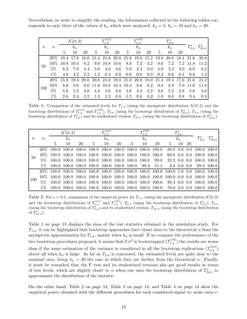
Nevertheless, in order to simplify the reading, the information collected in the following tables correspondsto only three of the values of k n which were analyzed: k n = 5, k n = 10 and k n = 20.n50100N (0, 2) T ∗(a)1,n T ∗(b)1,n T2,n∗α k n k n k n k n T3,n∗ T 3s,n∗5 10 20 5 10 20 5 10 20 5 10 2020% 19.4 17.6 16.0 21.4 21.6 20.0 21.6 19.0 15.2 19.8 20.8 18.4 21.6 20.810% 10.8 10.4 8.2 9.0 10.8 10.6 8.0 7.2 3.2 8.6 7.2 7.2 11.8 11.25% 8.2 7.0 4.4 5.0 4.0 4.6 5.0 2.4 0.0 4.0 3.2 3.0 6.0 6.21% 4.8 4.2 2.2 1.2 0.4 0.0 0.6 0.0 0.0 0.2 0.6 0.4 0.6 1.220% 15.0 19.4 20.0 20.8 21.0 19.0 21.0 20.8 18.0 21.4 19.4 17.6 21.6 21.210% 8.6 9.6 9.0 11.8 10.8 10.4 10.4 9.6 6.2 9.8 8.8 7.0 11.6 11.85% 5.6 5.2 4.0 4.4 4.6 3.6 3.6 3.4 2.2 4.6 5.2 2.8 5.6 5.61% 2.6 2.4 1.2 1.4 1.2 0.8 1.2 0.6 0.2 1.0 0.6 0.8 0.4 0.4Table 1: Comparison of the estimated levels for T 1,n (using the asymptotic distribution N (0, 2) and thebootstrap distributions of T ∗(a) ∗(b)1,n and T1,n ), T 2,n (using the bootstrap distribution of T2,n), ∗ T 3,n (using thebootstrap distribution of T3,n) ∗ and its studentized version, T 3s,n (using the bootstrap distribution of T3s,n).∗n50100N (0, 2)T ∗(a)1,n T ∗(b)1,n T2,n∗α k n k n k n k n T3,n∗ T 3s,n∗5 10 20 5 10 20 5 10 20 5 10 2020% 100.0 100.0 100.0 100.0 100.0 100.0 100.0 100.0 100.0 88.8 0.0 0.0 100.0 100.010% 100.0 100.0 100.0 100.0 100.0 100.0 100.0 100.0 100.0 60.8 0.0 0.0 100.0 100.05% 100.0 100.0 100.0 100.0 100.0 100.0 100.0 100.0 99.0 32.2 0.0 0.0 100.0 100.01% 100.0 100.0 100.0 100.0 100.0 100.0 100.0 99.4 51.4 3.4 0.0 0.0 99.4 100.020% 100.0 100.0 100.0 100.0 100.0 100.0 100.0 100.0 100.0 100.0 1.0 0.0 100.0 100.010% 100.0 100.0 100.0 100.0 100.0 100.0 100.0 100.0 100.0 100.0 0.0 0.0 100.0 100.05% 100.0 100.0 100.0 100.0 100.0 100.0 100.0 100.0 100.0 98.4 0.0 0.0 100.0 100.01% 100.0 100.0 100.0 100.0 100.0 100.0 100.0 100.0 100.0 70.0 0.0 0.0 100.0 100.0Table 2: For r = 0.5, comparison of the empirical power for T 1,n (using the asymptotic distribution N (0, 2)and the bootstrap distributions of T ∗(a) ∗(b)1,n and T1,n ), T 2,n (using the bootstrap distribution of T2,n), ∗ T 3,n(using the bootstrap distribution of T3,n) ∗ and its studentized version, T 3s,n (using the bootstrap distributionof T3s,n).∗Table 1 on page 13 displays the sizes of the test statistics obtained in the simulation study. ForT 1,n , it can be highlighted that bootstrap approaches have closer sizes to the theoretical α than theasymptotic approximation for T 1,n , mainly when k n is small. If we compare the performance of thetwo bootstrap procedures proposed, it seems that if σ 2 is bootstrapped (T ∗(b)1,n ) the results are worsethan if the same estimation of the variance is considered in all the bootstrap replications (T ∗(a)1,n )above all when k n is large. As far as T 2,n is concerned, the estimated levels are quite near to thenominal ones, being k n = 20 the case in which they are farther from the theoretical α. Finally,it must be remarked that the F–test and its studentized versions also get good results in termsof test levels, which are slightly closer to α when one uses the bootstrap distribution of T ∗ 3s,n toapproximate the distribution of the statistic.On the other hand, Table 2 on page 13, Table 3 on page 14, and Table 4 on page 14 show theempirical power obtained with the different procedures for each considered signal–to–noise ratio r.13