Bootstrap independence test for functional linear models

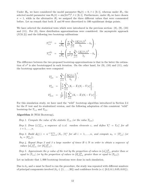
Under H 0 , we have considered the model parameter Θ 0 (t) = 0, t ∈ [0, 1], whereas under H 1 , theselected model parameter was Θ 1 (t) = sin(2πt 3 ) 3 , t ∈ [0, 1]. Furthermore, under H 0 we have chosenσ = 1, while in the alternative H 1 we assigned the three different values that were commentedbefore. Let us remark that both X and Θ were discretized to 100 equidistant design points.We have selected the statistical tests which were introduced in the previous section: (8), (9), (10)and (11). For (8), three distribution approximations were considered: the asymptotic approach(N (0, 2)) and the following two bootstrap calibrations⎛⎞T ∗(a) 11,n = √ ⎝ ṋ ∑k n(∆ ∗ n(ˆv j )) 2kn σ 2− k n⎠ ,T ∗(b)1,n =j=1⎛1√ ⎝nkn (ˆσ ∗ ) 2k n ∑j=1ˆλ j(∆ ∗ n(ˆv j )) 2ˆλ j− k n⎞⎠ .The difference between the two proposed bootstrap approximations is that in the latter the estimationof σ 2 is also bootstrapped in each iteration. On the other hand, for (9), (10) and (11), onlythe bootstrap approaches were computedT ∗ 2,n =T ∗ 3,n =k n ∑j=11∥n(∆ ∗ n(ˆv j )ˆλ j) 2,i=1T ∗ 3s,n = 1ˆσ ∗ ∥ ∥∥∥∥1nn∑(X i − ¯X)(Y i − Ȳ )ε∗ i∥ ,n∑(X i − ¯X)(Y i − Ȳ )ε∗ i∥ .i=1For this simulation study, we have used the “wild” bootstrap algorithm introduced in Section 2.4for the F–test and its studentized version, and the following adaptation of this consistent “wild”bootstrap for T 1,n and T 2,n .Algorithm 3 (Wild Bootstrap).Step 1. Compute the value of the statistic T 1,n (or the value T 2,n ).Step 2. Draw {ε ∗ i }n i=1i = 1, . . . , n.a sequence of i.i.d. random elements ε, and define Y∗i = Y i ε ∗ i for allStep 3. Build ∆ ∗ n(·) = n −1 ∑ ni=1 〈X i, ·〉Yi ∗ for all i = 1, . . . , n, and compute a n = |T1,n ∗ | (orb n = |T2,n ∗ |).Step 4. Repeat Steps 2 and 3 a large number of times B ∈ N in order to obtain a sequence ofvalues {a l n} B l=1 (or {bl n} B l=1 ).Step 5. Approximate the p–value of the test by the proportion of values in {a l n} B l=1greater than orequal to |T 1,n | (or by the proportion of values in {b l n} B l=1 greater than or equal to |T 2,n|).Let us indicate that 1, 000 bootstrap iterations were done in each simulation.Due to k n and α must be fixed to run the procedure, the study was repeated with different numbersof principal components involved (k n ∈ {1, . . . , 20}) and confidence levels (α ∈ {0.2, 0.1, 0.05, 0.01}).12