Bootstrap independence test for functional linear models

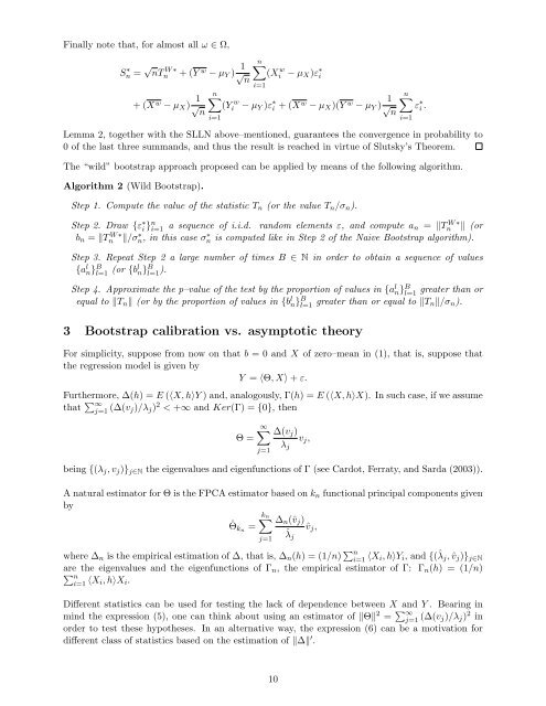
Finally note that, for almost all ω ∈ Ω,S ∗ n = √ nT W ∗n + (Y w − µ Y ) 1 √ n+ (X w − µ X ) 1 √ nn∑i=1n∑(Xi w − µ X )ε ∗ ii=1(Yi w − µ Y )ε ∗ i + (X w − µ X )(Y w − µ Y ) √ 1nn∑ε ∗ i .i=1Lemma 2, together with the SLLN above–mentioned, guarantees the convergence in probability to0 of the last three summands, and thus the result is reached in virtue of Slutsky’s Theorem.The “wild” bootstrap approach proposed can be applied by means of the following algorithm.Algorithm 2 (Wild Bootstrap).Step 1. Compute the value of the statistic T n (or the value T n /σ n ).Step 2. Draw {ε ∗ i }n i=1 a sequence of i.i.d. random elements ε, and compute a n = ‖TnW ∗ ‖ (orb n = ‖TnW ∗ ‖/σn, ∗ in this case σn ∗ is computed like in Step 2 of the Naive Bootstrap algorithm).Step 3. Repeat Step 2 a large number of times B ∈ N in order to obtain a sequence of values{a l n} B l=1 (or {bl n} B l=1 ).Step 4. Approximate the p–value of the test by the proportion of values in {a l n} B l=1greater than orequal to ‖T n ‖ (or by the proportion of values in {b l n} B l=1 greater than or equal to ‖T n‖/σ n ).3 Bootstrap calibration vs. asymptotic theoryFor simplicity, suppose from now on that b = 0 and X of zero–mean in (1), that is, suppose thatthe regression model is given byY = 〈Θ, X〉 + ε.Furthermore, ∆(h) = E (〈X, h〉Y ) and, analogously, Γ(h) = E (〈X, h〉X). In such case, if we assumethat ∑ ∞j=1 (∆(v j)/λ j ) 2 < +∞ and Ker(Γ) = {0}, thenΘ =∞∑j=1∆(v j )λ jv j ,being {(λ j , v j )} j∈N the eigenvalues and eigenfunctions of Γ (see Cardot, Ferraty, and Sarda (2003)).A natural estimator for Θ is the FPCA estimator based on k n functional principal components givenbyˆΘ kn =k n ∑j=1∆ n (ˆv j )ˆλ jˆv j ,where ∆ n is the empirical estimation of ∆, that is, ∆ n (h) = (1/n) ∑ ni=1 〈X i, h〉Y i , and {(ˆλ j , ˆv j )} j∈Nare the eigenvalues and the eigenfunctions of Γ n , the empirical estimator of Γ: Γ n (h) = (1/n)∑ ni=1 〈X i, h〉X i .Different statistics can be used for testing the lack of dependence between X and Y . Bearing inmind the expression (5), one can think about using an estimator of ‖Θ‖ 2 = ∑ ∞j=1 (∆(v j)/λ j ) 2 inorder to test these hypotheses. In an alternative way, the expression (6) can be a motivation fordifferent class of statistics based on the estimation of ‖∆‖ ′ .10