THE INSTABILITY ANALYSIS AND DIRECT NUMERICAL ...

To the Faculty of Washington State University:The members of the Committee appointed to examine the dissertation of XIN AIfind it satisfactory and recommend that it be accepted.__________________________________Chair______________________________________________________________________________________________________ii

ACKNOWLEDGMENTSI would like to express my gratitude to my advisor, Prof. Ben Q. Li, for hisdevoted guidance, continuous encouragement and support, and constructive suggestionsthroughout the course of this research.I would like to thank my committee members, Prof. B. R. Ramaprian, Prof.Clayton T. Crowe, Dr. Hong-Ming Yin and Dr. Prashanta Dutta, for their valuablesuggestions and timely assistance, which lead to significant improvements of thisdissertation.The financial support of this work from the NASA (Grant #: NAG8-1477 andNNM04AA17G) and the School of Mechanical and Materials Engineering is gratefullyacknowledged.I would like especially to thank my wife, Ying Zhu, for her love, support andunderstanding during the last several years. I would express my gratitude to my parents,my family and all my friends, for their continuous support and encouragement. I dedicatethe dissertation to all of them.iii

THE INSTABILITY ANALYSIS AND DIRECT NUMERICAL SIMULATION OFTURBULENT FLOWS IN ELECTROMAGNETICALLY LEVITATED DROPLETSAbstractby Xin Ai, Ph.D.Washington State UniversityMay 2004Chair: Ben Q. LiThe electromagnetic levitation has found a wide range of application in materialsprocessing community. The melt flow, which is driven by the induced Lorentz forces, isone of the important phenomena associated with the system. Experimental observationsand some numerical approximations have shown that melt flows in electromagneticallylevitated droplets are at least in a mildly turbulent regime. So far, little information on theinstability and turbulence phenomena in melt flows has been provided. Therefore, thestudies of the flow instability and turbulent flows inside the droplet generate informationthat is critical for both fundamental understanding and quantitative assessment of thissystem. The main objective of this research work is twofold. One is to present a linearstability analyses of melt flows in the magnetically levitated droplet, and the other is topredict the turbulent flows in the droplet by direct numerical simulation.Based on the high order finite difference scheme, we develop a parallelcomputing methodology for numerical simulation of two or three-dimensionallaminar/turbulent flows. This algorithm has been verified with the spectral-like accuracyiv

with superior computational efficiency and is used for the linear stability analysis anddirect numerical simulation in this work.The stability analysis is based on the solution of linearized Navier-Stokesequations in a spherical coordinate system. The perturbation equations are discretized bythe high order finite difference method, and the resulting eigenvalue problem is solved bythe linear fractional transformation with a full account of band matrix structure. Resultssuggest that the critical Reynolds number is below 100 and the most dangerous mode is k= 3. The discussion of physical mechanism of flow instability is presented.The flow transition and turbulent flows in electromagnetically levitated dropletsare studied by the direct numerical simulation. The typical Taylor-Gortler instability isidentified in the flow transition. Detailed information of turbulent flows in the droplet isprovided. Based on the database from direct numerical simulation, characteristic eddieson the free surface and inside the droplet, which are well agreed with experimentalobservations, are determined by using an orthogonal decomposition technique.v

TABLE OF CONTENTSPageACKNOWLEDGEMENTS ................................................................................................ iiiABSTRACT........................................................................................................................ivLIST OF TABLES .............................................................................................................. ixLIST OF FIGURES.............................................................................................................. xNOMENCLATURE.......................................................................................................... xviCHAPTER1. INTRODUCTION........................................................................................................11.1 Electromagnetic Levitation System .......................................................................11.2 Melt Flows in Electromagnetically Levitated Droplets .........................................41.3 Numerical Studies of Flow Instabilities and Turbulence.......................................81.4 Research Objectives .............................................................................................181.5 Scope of Present Research ...................................................................................202. PROBLEM STATEMENT ........................................................................................232.1 Introduction ..........................................................................................................232.2 Governing Equations............................................................................................242.3 Electromagnetic Forces........................................................................................252.4 Dimensionless Governing Equations in Spherical Coordinates...........................282.5 Boundary Conditions............................................................................................293. COMPUTATIONAL METHODOLOGY .................................................................313.1 Introduction ..........................................................................................................31vi

3.2 The High Order Finite Difference Method ..........................................................323.3 The Combined Runge-Kutta and Fractional Step Method...................................373.4 The Accuracy and Efficiency of the HOFD Method ...........................................403.5 The Parallel Algorithm.........................................................................................523.6 Summary ..............................................................................................................594. THE HIGH ORDER FININTE DIFFERENCE SCHEME FORINCOMPRESSIBLE FLOWS IN SPHERICAL COORDINATES..........................614.1 Introduction ..........................................................................................................614.2 Governing Equations............................................................................................624.3 Numerical Method................................................................................................645. THE LINEAR STABILITY ANALYSIS OF MELT FLOWS INELECTROMAGNETICALLY LEVITATED DROPLETS .....................................695.1 Introduction ..........................................................................................................695.2 Base Flow.............................................................................................................705.3 Linearized Perturbation Equations.......................................................................715.4 Numerical Methods..............................................................................................745.5 Results and Discussion.........................................................................................765.6 Summary ..............................................................................................................846. THE DIRECT NUMERICAL SIMULATION OF TURBULENCT FLOWS INELECTROMAGNETICALLY LEVITATED DROPLETS ...................................1166.1 Turbulent Flows in Electromagnetically Levitated Droplets .............................1166.2 Direct Numerical Simulation .............................................................................1206.3 Results and Discussion.......................................................................................134vii

6.4 Summary ............................................................................................................1497. CONCLUSION ........................................................................................................181BIBLIOGRAPHY .............................................................................................................184viii

LIST OF TABLES3.1 Comparisons in efficiency between the HOFD and spectral methods for the onedimensionalBurger’s equation problem .......................................................................493.2 Comparisons in efficiency between the HOFD and spectral methods for the twodimensionallid-driven cavity flow problem .................................................................523.3 Comparisons in accuracy between the HOFD and spectral methods for the twodimensionallid-driven cavity flow problem .................................................................523.4 CPU time (seconds) for a two-dimensional cavity driven flow solved with a singleprocessor........................................................................................................................543.5 CPU time at each time step of serial and parallel computing algorithms .....................585.1 Parameters for electromagnetic levitation calculations.................................................865.2 Mesh independency of the base flow calculations........................................................865.3 Comparisons of efficiencies for different eigenvalue solvers.......................................875.4 Mesh independency of the eigenvalue calculations ......................................................876.1 Mean values calculations with different sampling start time t 0 and sampling span T atthe location r = a, θ = 0.296875π and φ = 0................................................................1516.2 Mean values calculations with different sampling start time t 0 and sampling span T atthe point r = a, θ = 0.703125π and φ = 0. ...................................................................1516.3 Parameters in the direct numerical simulation of turbulent flows in anelectromagnetically levitated droplet of radius a. .......................................................151ix

LIST OF FIGURE1.1 Schematic representation of the TEMPUS electromagnetic levitation System...............21.2 Experimental results for the flow transition in an electromagnetically levitateddroplet, cited from Hyers et al. (2003)............................................................................72.1 Schematic representation of magnetic levitation system. The spherical coordinatesystem used for the numerical simulation is also shown ..............................................233.1 Exact solutions to the one-dimensional Burger's equation problem with periodicboundary conditions at different time: (a) t = 0 and (b) t = π/8. ...................................433.2 Spectral solutions to the one-dimensional Burger's equation with periodic boundaryconditions at t = π/8 with different mesh resolution: (a) N = 21, (b) N = 51 and(c) N = 101. ...................................................................................................................453.3 Finite difference solutions to the one-dimensional Burger's equation with periodicboundary conditions at t = π/8 with different mesh resolution: (a) N = 21, (b) N = 51and (c) N = 101..............................................................................................................463.4 Spectral and upwinding finite difference solutions to the one-dimensional Burger'sequation with periodic boundary conditions at t = π/8 and ν = 0.05 with differentmesh resolution: (a) N = 21, (b) N = 51 and (c) N = 101. .............................................483.5 Geometry and boundary conditions for a two-dimensional lid-driven cavity flow. .....503.6 Comparisons of the two-dimensional lid-driven cavity flow field calculations withdifferent numerical method: (a) the HOFD method and (b) the spectral method.........513.7 Schematic of the master-slave approach. ......................................................................553.8 Functions of tasks: (a) the master task and (b) the slave task. ......................................573.9 Performance of the parallel computing algorithm.........................................................595.1 Schematic representation of the electromagnetic levitation system..............................88x

5.2 Base flow structures on an axisymmetric plane of an electromagnetically levitateddroplet induced by electromagnetic fields with applied currents I = 200A: (a) twoloopbase flow and (b) four-loop base flow. .................................................................895.3 Eigenvalue spectrum of the base flow structures induced by electromagnetic fieldswith applied currents I = 20A: (a) two-loop base flow and (b) four-loop base flow. ...905.4 Stability diagram for two-loop melt flows in an electromagnetically levitated droplet:(a) critical Reynolds number and (b) critical electrical current. ...................................915.5 Contours of perturbed velocity u r´ of the leading mode (Re = 95.0269) on anaxisymmetric plane for the two-loop base flow in an electromagnetically levitateddroplet: (a) t = t 1 , (b) t = t 1 +T/4, (c) t = t 1 +T/2 and (d) t = t 1 +3T/4. ..............................925.6 Contours of perturbed velocity u θ´ of the leading mode (Re = 95.0269) on anaxisymmetric plane for the two-loop base flow in an electromagnetically levitateddroplet: (a) t = t 1 , (b) t = t 1 +T/4, (c) t = t 1 +T/2 and (d) t = t 1 +3T/4. ..............................935.7 Contours of perturbed velocity u φ´ of the leading mode (Re = 95.0269) on anaxisymmetric plane for the two-loop base flow in an electromagnetically levitateddroplet: (a) t = t 1 , (b) t = t 1 +T/4, (c) t = t 1 +T/2 and (d) t = t 1 +3T/4. ..............................945.8 Evolution of the perturbation energy of the leading mode with the time for the twoloopmelt flow in an electromagnetically levitated droplet: (a) Re = 95.0269 and (b)Re = 101.0531. ..............................................................................................................955.9 Contours of kinetic energy of the leading mode (Re = 95.0269) on an axisymmetricplane for the two-loop melt flow in an electromagnetically levitated droplet: (a) t = t 1 ,(b) t = t 1 +T/4, (c) t = t 1 +T/2 and (d) t = t 1 +3T/4. ...........................................................965.10 Contours of energy production of the leading mode (Re = 95.0269) on anaxisymmetric plane for the two-loop melt flow in an electromagnetically levitateddroplet: (a) t = t 1 , (b) t = t 1 +T/4, (c) t = t 1 +T/2 and (d) t = t 1 +3T/4. ..............................97xi

5.11 Contours of energy dissipation of leading mode (Re = 95.0269) on an axisymmetricplane for the two-loop melt flow in an electromagnetically levitated droplet: (a) t = t 1 ,(b) t = t 1 +T/4, (c) t = t 1 +T/2 and (d) t = t 1 +3T/4. ...........................................................985.12 Stability diagram for four-loop melt flows in an electromagnetically levitateddroplet: (a) critical Reynolds number and (b) critical electrical current. ......................995.13 Contours of perturbed velocities of the leading mode (Re = 38.8010) on anaxisymmetric plane for the four-loop base flow in an electromagnetically levitateddroplet at t = t 1 : (a) u r´, (b) u θ´ and (c) u φ´...................................................................1015.14 Contours of perturbed energy of the leading mode (Re = 38.8010) on anaxisymmetric plane for the four-loop melt flow in an electromagnetically levitateddroplet at t = t 1 : (a) kinetic energy, (b) energy productionand (c) energy dissipation ...........................................................................................1035.15 Four-loop flow structure on an axisymmetric plane of an electromagneticallylevitated droplet induced by a quadrupole electromagnetic field with applied currentsI = 200A and a larger distance d = 5. ..........................................................................1045.16 Stability diagram for the four-loop flow structure in an electromagnetically levitateddroplet with a larger distance d = 5: (a) critical Reynolds number and (b) criticalelectrical current..........................................................................................................1055.17 Contours of perturbed velocities of the leading mode (Re = 44.6678) on anaxisymmetric plane for the four-loop base flow in an electromagnetically levitateddroplet with a larger distance d = 5 at t = t 1 : (a) u r´, (b) u θ´ and (c) u φ´. .....................1075.18 Contours of perturbed energy of the leading mode (Re = 44.6678) on anaxisymmetric plane for the four-loop base flow in an electromagnetically levitateddroplet with a larger distance d = 5 at t = t 1 : (a) kinetic energy, (b) energy productionand (c) energy dissipation. ..........................................................................................109xii

5.19 Two-loop flow structure on an axisymmetric plane of an electromagneticallylevitated droplet with a solid surface induced by a dipole electromagnetic field withapplied currents I = 200A............................................................................................1105.20 Stability diagram for the two-loop flow structure in an electromagnetically levitateddroplet with a solid surface: (a) critical Reynolds number and(b) critical electrical current. .......................................................................................1115.21 Contours of perturbed velocities of the leading mode (Re = 108.1728) on anaxisymmetric plane for the two-loop base flow in an electromagnetically levitateddroplet with a solid surface at t = t 1 : (a) u r´, (b) u θ´ and (c) u φ´ ..................................1135.22 Contours of perturbed energy of the leading mode (Re = 108.1728) on anaxisymmetric plane for the two-loop base flow in an electromagnetically levitateddroplet with a solid surface at t = t 1 : (a) kinetic energy, (b) energy production and (c)energy dissipation........................................................................................................1156.1 Two-point correlations of turbulent flows in an electromagnetically levitated dropletat r = 0.921875a and two different θ locations:(a) θ = 0.3125π and (b) θ = 0.6875π...........................................................................1526.2 Two-point correlations of turbulent flows in an electromagnetically levitated dropletat r = 0.15625a and two different θ locations:(a) θ = 0.3125π and (b) θ = 0.6875π...........................................................................1536.3 One-dimensional energy spectra for turbulent flows in an electromagneticallylevitated droplet with a mesh 65 × 65 × 131 in r, θ, and φ directions at two differentlocations: (a) r = 0.921875a, θ = 0.3125π and (b) r = 0.921875a, θ = 0.6875π.........1546.4 One-dimensional energy spectra for turbulent flows in an electromagneticallylevitated droplet with a mesh 65 × 65 × 131 in r, θ, and φ directions at two differentlocations: (a) r = 0.15625a, θ = 0.3125π and (b) r = 0.15625a, θ = 0.6875π.............155xiii

6.5 One-dimensional energy spectra for turbulent flows in an electromagneticallylevitated droplet with a mesh 91 × 91 × 131 in r, θ, and φ directions at two differentlocations: (a) r = 0.921875a, θ = 0.3125π and (b) r = 0.921875a, θ = 0.6875π.........1566.6 One-dimensional energy spectra for turbulent flows in an electromagneticallylevitated droplet with a mesh 91 × 91 × 131 in r, θ, and φ directions at two differentlocations: (a) r = 0.15625a, θ = 0.3125π and (b) r = 0.15625a, θ = 0.6875π.............1576.7 Instantaneous velocity vectors on the free surface of an electromagnetically levitateddroplet at Re = 95: (a) three-dimensional plot and (b) φ-θ plane projection. .............1586.8 Instantaneous velocity vectors on the free surface of an electromagnetically levitateddroplet with at Re = 521: (a) three-dimensional plot and (b) φ-θ plane projection. ...1596.9 Instantaneous velocity vectors on the free surface of an electromagnetically levitateddroplet with at Re = 1491: (a) three-dimensional plot and (b) φ-θ plane projection. .1606.10 Contours of initial normal vorticity ω r on the free surface of an electromagneticallylevitated droplet at Re = 1491: (a) three-dimensional plot and (b) φ-θ planeprojection.....................................................................................................................1616.11 Contours of instantaneous normal vorticity ω r on the free surface of anelectromagnetically levitated droplet at Re = 1491: (a) three-dimensional plot and (b)φ-θ plane projection. ...................................................................................................1626.12 Three-dimensional mean velocity field of melt flows in an electromagneticallylevitated droplet at Re = 95: (a) cutting on planes φ=0, φ=π/2 and θ=π and (b) cuttingon planes φ=π, φ=2π/2 and θ=π/2. ..............................................................................1636.13 Three-dimensional mean velocity field of melt flows in an electromagneticallylevitated droplet at Re = 521: (a) cutting on planes φ=0, φ=π/2 and θ=π and (b)cutting on planes φ=π, φ=2π/2 and θ=π/2...................................................................1646.14 Three-dimensional mean velocity field of melt flows in an electromagneticallylevitated droplet at Re = 1491: (a) cutting on planes φ=0, φ=π/2 and θ=π and (b)cutting on planes φ=π, φ=2π/2 and θ=π/2...................................................................165xiv

6.15 Two-dimensional mean velocity field of melt flows in an electromagnetically−2levitated droplet at Re =521 ( U max = 4.06 × 10 m / s ). .............................................1666.16 Two-dimensional mean velocity field of melt flows in an electromagnetically−2levitated droplet at Re =1491 ( U max = 11.14 × 10 m / s ). ..........................................1676.17 Isosurfaces of instantaneous normal vorticity ω r =±1.5 inside an electromagneticallylevitated droplet at Re = 1491. ....................................................................................1686.18 Contours of root-mean-square velocity fluctuations on the free surface of anrmsrmselectromagnetically levitated droplet at Re = 1491: (a) u θand (b) u φ..................1696.19 Contours of turbulent energy on the free surface of an electromagnetically levitateddroplet at Re = 1491: (a) kinetic energy k and (b) viscous dissipation ε. ...................1706.20 Contours of the ratio of the eddy viscosity and the laminar viscosity on the freesurface of an electromagnetically levitated droplet at Re = 1491...............................1716.21 Distributions of root-mean-square velocity fluctuations along the r direction (θ =π/4) of an electromagnetically levitated droplet at Re = 1491....................................1726.22 Distributions of turbulent energy along the r direction (θ = π/4) of anelectromagnetically levitated droplet at Re = 1491: (a) kinetic energy k and (b)viscous dissipation ε....................................................................................................1736.23 Distributions of turbulent energy derivatives along the r direction (θ = π/4) of anelectromagnetically levitated droplet at Re = 1491: (a) ∂k/∂r and (b) ∂ε/∂r...............1746.24 Distribution of the ratio of the eddy viscosity and the laminar viscosity along the rdirection (θ = π/4) of an electromagnetically levitated droplet at Re = 1491.............1756.25 Side view (x-z plane) of two-dimensional zero-phase characteristic eddy on the freesurface of an electromagnetically levitated droplet with Re =1491............................1776.26 Side view (x-z plane) of two-dimensional zero-phase secondary eddy on the freesurface of an electromagnetically levitated droplet with Re = 1491...........................1796.27 Isosurfaces of normal vorticity ω r =±1.5 of the characteristic eddies of anelectromagnetically levitated droplet at Re = 1491.....................................................180xv

NOMENCLATUREaBDEfFHIJkpPReRmuU(x, y, z)(r, θ, φ)Radius of dropletMagnetic fieldElectric displacementElectric fieldFrequencyLorentz forceMagnetic densityElectrical currentCurrent densityWave number or Kinetic energyPressureBase flow pressureReynolds numberMagnetic Reynolds numberVelocity fieldBase flow velocity fieldCartesian coordinatesSpherical coordinatesGreekδ Electrical skin depth ( = 2 / ωµ σ )δ0εViscous dissipationxvi

ηλKolmogorov length scaleTaylor length scaleµ Viscosity of fluidµ 0 Magnetic permeability of free spaceρστωDensity of fluidElectrical conductivityReynolds stressAngular frequency or vorticitySubscriptsrθφComponent in the r directionComponent in the θ directionComponent in the φ directionSuperscripts* Complex conjugate′ Perturbed fieldxvii

CHAPTER ONEINTRODUCTION1.1 Electromagnetic Levitation SystemThe electromagnetic levitation system is an important containerless device for thefundamental scientific research in microgravity. The system has been applied in materialsprocessing community for multifarious purposes such as to obtain materials of ultrapurity,to understand the fundamental laws governing the microstructure developmentsuch as nucleation and grain growth during metal solidification, and to measure thermophysicalproperties of highly corrosive and/or undercooled melts (Flemings et al. 1996,Herlach et al. 1986, Herlach 1991, Herlach et al. 1991, Johnson et al. 1996, Rhim 1997and Sauerland et al. 1991). The very nature of the complex system associated withelectromagnetic levitation has also triggered inquisitive minds into understanding ofsome interesting phenomena such as melt flow, free droplet deformation and oscillationand heat transfer (Bratz and Egry 1995, El-Kaddah and Szekely 1983, Li 1993, Li 1994,Li and Song 1998, and Mestel 1982).The containerless device is to levitate a working sample, melt or solid, in the airagainst gravity so that it is free from wall related contamination. Under the microgravitycondition, the system is exploited to confine the sample from drifting in space. Withoutcontact with a solid wall, a levitated sample can be allowed to cool far below its meltingpoint but still remains liquid, which is called undercooling. With a substantialundercooling, simultaneous nucleation may occur in the melt, followed by grain crystal,thereby producing a solid with a microstructure consisting of extremely fine-sized grains.1

A containerless processing system also offers a uniquely useful means by which thethermophysical properties of high melting point and corrosive melts can be measuredwithout interference from the container walls. Moreover, it seems to be the onlytechnique for measuring the physical properties of the undercooled melts (Rhim 1997).13.549.5104Figure 1.1 Schematic representation of the TEMPUS electromagnetic levitation System.The concept of electromagnetic levitation is based on the Faraday’s law. Eddycurrents are induced in the electrically conducting specimen when imposing a timevaryingmagnetic field. The interaction between the eddy current and the total magneticfield, which includes the self-induced and the imposed magnetic fields, gives arise to the2

Lorentz forces in the specimen. The specimen can be levitated if the magnetic forces arestrong enough. Meanwhile, Joule heating, which comes from the self-interaction of theinduced eddy currents, melts the sample.The TEMPUS (Tiegelfreies Elektromagnetisches Prozessieren UnterSchwerelosigkeit; containerless electromagnetic processing under weightlessness) deviceis an electromagnetic levitation system, which was developed by German researchers andspecially designed for the microgravity applications (Flemings et al. 1996). The devicehas been flown on several space shuttle missions and got some very useful results(Flemings et al. 1996). The schematic representation of this system is shown in figure1.1. A spherical sample is surrounded by two sets of coils, the inner heating coils and theouter positioning coils. The currents in the positioning coils are out of phase and induce aquadruple magnetic field. The quadruple magnetic field generates a magnetic potentialwell to confine the sample in space. The heating coils have the higher currents with ahigher frequency than positioning coils. The in-phase currents in the heating coils inducea dipole magnetic field. This strong dipole field creates the induction heating to meltfluids, and generates the Lorentz forces to drive motions of the melts and causes thedeformation of the droplet (El-Kaddah and Szekely 1983).There are numerous interesting physics issues coming along with theelectromagnetic levitation system, e.g., the electromagnetic levitation melting processes,the electromagnetically induced deformation, the Joule heating, force distribution, shapeoscillation, heat transfer in the liquid droplets, and the fluid flows in the levitationsystems. Since the pioneering research on the subject was conducted by Okress et al.(1952), extensive research work on these issues has been published by using analytical,3

perturbation and numerical methods (Bayazitoglu and Sathuvalli 1994, Bayazitoglu andSathuvalli 1996, Bayazitoglu et al. 1996, Li 1993, Li 1994, Li and Song 1998, Mestel1982, Zong et al. 1992 and Zong et al. 1993).1.2 Melt Flows in Electromagnetically Levitated DropletsIn this work, internal melt flows in electromagnetically levitated droplets arestudied. The internal fluid flow in the droplet is driven by the magnetic forces and theflow pattern is characterized by two anti-rotating recirculating loops. Many experimentshave suggested that studies of internal flows are crucial for understanding theelectromagnetic levitation system. Egry et al. (1998) have reported to use the oscillatingdrop technique to measure the viscosity of eutectic Pd 78 Cu 6 Si 16 under microgravityconditions. It has been found that if the electromagnetic field is strong enough to induceturbulent flows in the sample, the viscoelastic effect associated with the turbulentviscosity provides additional damping of the surface oscillations. Therefore, in theturbulent regime, the oscillating drop technique might be failed to measure the trueviscosity of the material property. Hofmeister and Bayuzick (1999) have analyzed theliquid-to-solid nucleation experiments on pure zirconium. Their studies showed that thereis no evidence for fluid flow effects on nucleation of supercooled zirconium for internalflows from 5 to 43cm/s. At flows greater than 50cm/s, cavitations in fluids areintroduced, which will limit the undercooling. Therefore, knowledge of the melt flowinstability and turbulence in electromagnetically levitated droplets is of both fundamentaland practical significance.4

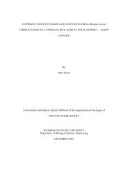
In 1952, Okress et al. (1952) first reported the instability phenomena in levitatedsamples. In their experiment, it is found that under certain conditions the samples start torotate and oscillate. Lee et al. (1991) and Anilkumar et al. (1993) had some furtherexperimental studies in these phenomena. It should be noting that all these experimentsare only concerned with the instabilities related to the shape oscillation but not thehydrodynamic instability in levitated samples. Not until recently, an experimentalinvestigation of the laminar-turbulent transition in an electromagnetically levitateddroplet has been reported by Hyers et al. (2003). The experiment is taken on the MSL-1(First Microgravity Science Laboratory) mission of Space Shuttles in 1997. In theexperiment, a droplet of palladium-silicon alloy was electromagnetically levitated withthe TEMPUS device. Since the alloy sample is opaque and very small, it is impossible toobserve flows inside the sample by means of current measurement techniques. In theexperiment, motions of the tracer particles on the sample surface were observed, whichsomehow gives us information of the flows inside the droplet.Experimental results (see figure 1.2a) show that when the temperature of thesample is at T = 1203-1212K, a steady laminar flow pattern is observed. The tractorparticles show that the stagnation line is very steady and located at the equator of thesample. This refers that a two anti-rotating recirculating flow structure is inside thedroplet. As the sample is further heated (see figure 1.2b) the tracer particles in thestagnation line start to oscillate up and down about the equator. The onset of thisoscillation is at about T = 1225K. It indicates that instability flow structures in the dropletare undergoing. As the heating continuous, the temperature in the flow keeps increasingand the amplitude of the oscillation increases. Figure 1.2(c) shows when the temperature5

is above T = 1240K, the stagnation line is no longer visible, and apparent chaotic swirlingeddies are observed on the free surface of the droplet. The observed chaotic motion onthe surface exhibits the turbulent flows inside the droplet.This experiment clearly demonstrates the flow transition from laminar to turbulentflows inside the electromagnetic levitated droplet, and shows flow instabilities of a pairof anti-rotating toroidal flow structures lead to the emergence of turbulent flows insidethe droplet. The reported experimental results provide some useful information on thedesign and control of electromagnetic processing systems, e.g., how to avoid turbulentflows in applications of electromagnetic levitated systems, and how to take advantage ofthe melt turbulence in the case of electromagnetic stirring. It is worth noting that thisexperimental technique has two unavoidable defects, i.e., the information of turbulentflows inside the droplet can only be referred from motions of the tracer particles on thefree surface of the droplet and cannot be observed directly, and the cost of such anexperiment is very high.With the development of the numerical techniques and computer technology, thenumerical simulation has become a powerful tool to provide data needed by fundamentalresearch and industry applications. In this work, a numerical method is developed fornumerical studies of the melt flow instabilities and transition from laminar to turbulentflows in electromagnetically levitated droplets, and a direct numerical simulation iscarried out for an accurate resolution of turbulence in the droplet. We expect this work toprovide a useful numerical technique for electromagnetic levitation system design andcontrol.6

Re=451 Re=452 Re=457 Re=461 Re=466 Re=472 Re=477 Steady LaminarFlow(a) Laminar flow at T = 1203-1212K, respectively, left to right. The flow pattern remains the same as the flow accelerates over thelaminar region. The tracer particles collect into the stagnation line on the equator. Small perturbations in the flow pattern damp overtime. Frames are 1/15 sec apart.Re=523 Re=528 Re=534 Re=539 Re=545 Re=551 Re=556 OscillatoryFlow(b) Oscillatory flow at T = 1226-1235K, respectively, left to right. As the temperature rises, the oscillations in the stagnation linedevelop, as shown by the tracer particles. Frames are 1/15 sec apart.Re=590 Re=594 Re=596 Re=599 Re=601 Re=605 Re=608 Turbulent Flow(c) Turbulent flow at T = 1244-1249K, respectively, left to right. At the higher velocity, the line of tracers disperses as the flowbecomes turbulent. The tracer particles follow random swirling paths across the surface of the droplet. Frames are 1/30 sec apart.Figure 1.2 Experimental results for the flow transition in an electromagnetically levitated droplet, cited from Hyers et al. (2003).7

1.3 Numerical Studies of Flow Instabilities and TurbulenceIt is well known that the Navier-Stokes (NS) equations are fundamental toanswers to all fluid dynamic problems. These equations are the most widely studiedequations in the applied physics. The range of validity of NS equations is only limited bythe model being used for the viscous stresses, for example, Newtonian, non-Newtonian,turbulent eddies, etc. For an incompressible Newtonian fluid flow, the conservation lawsfor mass and momentum govern the fluid motion, and the NS equations can be written as∇ ⋅u = 0(1.1)∂ 2uρ + ρu⋅∇u= −∇p+ µ ∇∂tu + F(1.2)where u denotes the instantaneous velocity field, p is the hydrodynamic pressure, F is theexternal force, ρ is the fluid density, µ is the dynamic viscosity, and t is the time. Theflow field is determined by solutions of the above governing equations and thecorresponding initial and boundary conditions.1.3.1 Linear stability analysisTo investigate the flow instability and transition from laminar to turbulent flows,the problem of hydrodynamic stability is introduced. The problem is defined as follows:Given U and P are steady state solutions of equations (1.1) and (1.2), we seek solutionsof above system in the form of8

+∑ ∞k=1( ) ( k )u = U ε k u(1.3)+∑ ∞k=1( ) ( k )p = P εk p(1.4)where ε is a small constant number, u (k) and p (k) are the k th order disturbances deviatedfrom the steady state solutions. If these disturbances approach zero as time t goes toinfinity, then the flow is stable, otherwise the flow is unstable.Since generally it is very difficult and costly to obtain those solutions by solvingnonlinear NS equations directly, the linear stability theory is used. The theory is based onthe assumption that for small disturbances, the nonlinear NS equations can be linearized,and the high order disturbances and their derivatives therefore can be neglected. Theresulting linear system therefore can be expressed as(1)∇ ⋅u = 0(1.5)∂uρ∂t(1)+ ρU⋅∇u(1)+ ρu(1)⋅∇U= −∇p(1)+ µ ∇2u(1)(1.6)It is worth noting that solutions of above system have an exponential time factor exp(σt),where σ is a complex parameter. If the real part of σ is negative, all disturbances are todie out as time goes by and the flow is said to be stable. If the real part of σ is positive,the flow is then said to be unstable. In the case that σ is real, the flow is in the neutralstate. Therefore, the problem of hydrodynamic stability finally leads to a characteristic-9

value problem, where the characteristic values of parameter σ are solved to identify theflow stability.There exists abundant literature on the linear stability analyses of wall-boundedshear flows and flow transitions from laminar to turbulent regimes. The most widelystudied cases include the Couette, Poiseuille and channel flows. The methodologies usedfor the flow stability study have been well established, starting from the early days usingthe singular perturbation method to relatively more recently using the spectral basednumerical method. These studies have established basic mechanisms by which theinstability sets in and gradually develops into turbulence. A comprehensive review of theresearch work on the subject has been documented by Drazin and Reid (1981). Despite ofits mathematical limitation, the linear stability analysis has been widely used as a firststep to investigate the flow stability problems, and its interest in these problems is stillgrowing (Ding and Kawahara 1999, Priede and Gerbeth 1999, Shatrov et al. 2001)because of its fundamental and practical importance.In this work, electromagnetically levitated droplets provide a new system for thelinear stability study of flow transition to turbulence. To the authors’ knowledge,however, little numerical work has been done to address the instability of melt flows inelectromagnetically levitated droplets, in spite of their fundamental and engineeringimplications. So far, a linear stability analysis presented by Shatrov et al. (2001) is theonly work we can find. In the paper, a three-dimensional linear stability analysis of themelt flow inside the droplet is conducted with a pseudo-spectral method. They found outthat for this problem the critical Reynolds number is below 100 and the most unstableazimuthal wave number is 3. While the existing literature is certainly helpful in providing10

some basic numerical results of the stability of the type of flows, the underlying physicsthat governs the flows and their instability is barely studied. Of particular importance arethe questions of how electromagnetically induced flows are affected by induction fieldparameters and of how these types of flows differ from those types of flows that havebeen widely studied. Hyers et al. (2003) addressed that the most unstable azimuthal wavenumber reported by Shatrov et al. (2001) does not agree with their experimentalobservations. Therefore, a comparison of our results obtained from linear stabilityanalysis with experimental studies is of importance. In this work, a linear stabilityanalysis of the melt flow in the droplet is presented and answers to the above questionsare given.1.3.2 Numerical simulation of NS equationsWhile the linear stabiliy analysis may give information on the flow instability andtransition to turluence, to further study the turbulence in the electromagnetically levitateddroplet, the nonlinear NS equations need to be solved. So far, established techniques fornumerical solutions of NS Euations include: (1) Numerical simulation of Reynoldsaveraged NS equations (RANS) or time-dependent Reynolds averaged NS equations(TRANS), (2) Large eddy simulation (LES), and (3) Direct numerical simulation (DNS).The computational cost of the solution increases from (1) to (3), yet the validation of theirapplicabilities decreases from (1) to (3) because of those assumptions applied in the threetechniques.The RANS/TRANS are the most popular form of the NS equations used in thecomputational fluid dynamics (CFD) area. In most industrial flows, it is indeed11

impossible to have a direct solution of the NS equations. In fact, in unsteady turbulentflows, flow properties such as the kinetic energy and heat are transported by turbulence.The turbulent transport occurs on length scales greater than the ones where viscousdissipation and heat conduction occur. Therefore, it is possible to average the goveriningequations to obtain approximate solutions. The velocity and pressure of flow fieldsdepend on the space and time. The instananuous flow field (u, p) can be decomposed intoa time mean component field (U, P) and a time dependent fluctuation field ( u ~ , ~ p ), i.e.,u = U + u~(1.7)p = P + ~ p(1.8)Applying decompositions (1.7) and (1.8) into equations (1.1) and (1.2), and doing thetime average, we have the NS equations in the TRANS form as follows∇ ⋅ U = 0(1.9)Uρ + ρU⋅∇U= −∇P+ µ ∇∂t∂ 2U + ∇ ⋅ τ + F(1.10)where components of the Reynolds stress tensor τ are τ = −ρ u ~ u ~ . The Reynolds stresstensor represents the mean rate of momentum transfer due to turbulence. The diagonalcomponents of τ are normal stresses, which usually contribute little to the transport of themean momentum in turbulent flows. The off-diagonal terms of τ are called shear stresses,which play a dominant role in the theory of mean momentum transfer by turbulence.ijij12

Since the Reynolds stresses are additional unknowns with respect to the NS equations,the system of TRANS equations is not well defined. This requires an addition of arelationship to the Rynolds stress τ as a function of the mean flow variables (U, P), whichis well known as turbulent models.In general, turbulence closure models for the TRANS equations are based on adimensional analysis of the Reynolds stress tensor.The Reynolds stress tensor can beexpressed as a function of the velocity fluctuation variance which relates to the turbulentkinetic energy. To model the Reynolds stress tensor, the interaction of the turbulentkinetic energy with the mean flow is examined. Such interaction is described by theReynolds averaged turbulent kinetic energy equation (Tennekes and Lumley 1972).Tubulent models widely being used include: (1) Zero equation B-L model (Baldwin andLomax 1978), (2) One equation B-B (Baldwin and Barth 1990) and S-A (Spalart andAllmaras1992) models, (3) One and half equation J-K (Johnson and King 1985) model,and (4) Two equation k-ε (Launder and Spalding 1974) and k-ω (Wilcox 1994) models.The role of turbulence is strongly related to the Reynolds number. The high Reynoldsnumber flows are much less affected by turbulence models, unless they feature extensiveareas of separated flow. In spite of limitations of these approximate turbulent models,nowadays the RANS/TRANS method is still the most popular technique for solving theturbulent flows in industry applications because of its high efficiency and relatively highaccuracy.As we have mentioned, many experimental observations have suggested thatunder certain levitation conditions, the fluid motion in a levitated droplet is within theturbulent regime. Some previous results obtained from the approximate turbulence13

calculations for this system suggest that the ratio of the eddy viscosity over the dynamicviscosity due to the turbulence is on the order of 10 to 40 (Li 1994, Zong et al. 1992,Zong et al. 1993). Therefore, a description of the mild turbulence would require aturbulent closure models. So far turbulent models developed for turbulent flows inelectromagnetically levitated droplets are either based on a pseudo-laminar assumptionwhere the laminar viscosity is increased to account for turbulence or based on the popularengineering k-ε types of empirical turbulence models. Neither of the above is deemedadequate, although they serve as some sort of approximations and widely used to predictthe melt flows in magnetically levitated droplets (Zong et al. 1992, Zong et al. 1993). Asis known, most of turbulent models are developed for the high Reynolds numberturbulent flows, and there is a lack of adequate models for the mild turbulent flowsencountered in magnetically levitated droplets. Therefore, to precisely predict theturbulent flows, the direct numerical simulation of the Navier-Stokes equations is needed.1.3.3 Direct numerical simulationIn turbulent flows, turbulent eddies with all possible wavelengths are all included.Therefore, the numerical simulation of the NS equations, which have less assumption, isexpected to have a better resolution of turbulent flows. Numerical simulations ofturbulent flows represent a very challenging task, because of the huge requiredcomputing resources. With the increase in computing power over the pasting decade,numerical computation of the NS equations is possible although it is still far fromadequate.14

The large eddy simulation (LES) is a method between the approximate simulationand exact simulation of the NS equations. Roughly speaking, the computational meshused in this method is much denser than those used in the RANS/TRANS method, and ismuch coarser than those used in the direct numerical simulation. Therefore, this methodis much more accurate than the approximate method such as RANS and TRANS, since itcan accurately predict the large-scale turbulent structures, which are the most importantin the transport quantities. On the other hand, since the small-scale turbulence needs to bemodeled, this method is not as accurate as the DNS method. In general, the small-scaleturbulent structures are represented by sub-grid stress models, which include theSmagorinsky eddy viscosity models (Smagorinsky 1963), dynamic sub-grid models(Germano et al. 1991), mixed models (Bardina et al. 1980) and backscatter models(Mason and Thomson 1992). The LES method extends the utility of the DNS method forpractical applications by intentionally leaving the smallest turbulent structures spatiallyunder-resolved. Since a relatively coarser grid can be employed, a large savings incomputer resources is expected to the LES method. This makes this method possible forsolving problems with more complex geometric configurations (Akselvoll and Moin1996, Haworth and Jansen 2000) or at relatively high Reynolds numbers (Breuer 2000,Cabot and Moin 2000).Direct numerical simulation (DNS) is an exact solution of the NS equations,which is capable of resolving all possible turbulent scales from the smallest one to thelargest one without requiring any kind of additional closure models. It is well agreed thatresults from a DNS and an experiment are comparable, and the DNS technique has nolimitations of the experimental apparatus. Moreover, this approach does not suffer from15

any drawbacks like other methods, and it should be the easiest one to implement. As wehave mentioned before, turbulence contains eddy structures with different length scales,therefore the mesh should be dense enough to resolve the smallest eddy structures, andthe computational domain should be large enough to capture largest eddy structures,which are characterized by the largest scales of length L, time t and velocity U.According to the Kolmogorov universal equilibrium (Gibson and Schwartz 1963),the smallest eddies are characterized by Kolmogorov micro-scales of length η, time τ andvelocity v which are defined by3 1/ 4η = ( ν / ε ) ,1/ 2τ = ( ν / ε ) ,1/ 4v = (νε )(1.11)where ε is the dissipation rate per unit mass and ν =µ /ρ is the kinematic viscosity. Theratio of the largest and smallest characteristic scales therefore can be estimated by(Tennekes and Lumley 1972)3/ 4L /η ~ Re ,1/ 2t /τ ~ Re(1.12)where the Reynolds number Re is defined by Re = ρUL/µ. Thus, the number of the gridpoints N required by the DNS method for a three-dimensional turbulent flow calculationis proportional to Re 3/4 , the time step used in the DNS method has to be less than Re -1/2 ,and hence the time cost increases rapidly wit the Reynolds number approximately as Re 3 .In industrial applications, typical Reynolds number are 10 6 or above. Therefore, the directnumerical simulation requires a sufficiently large computational domain, a very dense16

mesh and a very small time step, and thus presently the DNS method is only confined tosimple problems and relatively small Reynolds numbers. With the recent advances incomputer hardware, the direct numerical simulation of turbulence has gained more andmore attention though it is still a computationally intensive task.Until the recent past, the spectral method has been the choice for direct numericalsimulations of turbulent flows and transition from laminar to turbulent flows, pioneeredby Orszag and Patterson (1972) and Rogallo (1981) for homogeneous turbulent flows.Based on the global series expansion, the spectral method provides perhaps the highestorder of numerical approximation among all the available techniques such as finitevolume and finite elements (Adams and Kleiser 1996, Pruett and Zang 1992, Rai andMoin 1993, and Rist and Fasel 1995).For direct numerical simulations of the inhomogeneous turbulent flows, theFourier representations cannot be used in directions of inhomogeneity where the periodicboundary conditions are not satisfied. Kim et al. (1987) presented a pseudo-spectralmethod to solve the inhomogeneous channel, in which the Fourier representations areperformed in the spanwsie and streamwise directions, and the Chebyshev polynomials arerepresented in the cross-stream direction.As the applications of the direct numerical simulation are extended, there havealso been many attempts that combine the spectral accuracy and features of finiteelements to provide a more flexible treatment of irregular geometry and/or bettercomputational speed. Few attempts have also been made to apply the finite volumemethod to carry out the direct simulation of turbulence. Because the finite volumemethod is a lower order method, the massive grid points required by resolving the needed17

accuracy for describing the turbulent flow behavior result in the use of extensivecomputing power. This makes the standard finite volume method less attractive than thespectral method for high accuracy computations.Recently, the high order finite difference methods (Christie 1985, Lele 1992,Sabau 1999) have emerged as one of better alternatives for the direct simulation ofturbulent flows. The method possesses the spectral-like accuracy, and has flexibility withmesh geometry and a variety of boundary conditions. Compared with the standard finitevolume method, the high order finite difference schemes provide substantially improvedaccuracy that is needed to capture a wide range of spatial scales that are inherent inturbulent flows and transition flows (Carpenter et al. 1993 and Zhong 1998).In this work, we present a direct numerical simulation of turbulence in theelectromagnetically levitated droplet. So far no work has been published yet in spite of itsimportance on fundamental research and industry applications. It is a challenging workbecause of its different geometric configuration and a more complicated flow feature.1.4 Research ObjectivesIn this work, we develop a numerical method to analyze problems of melt flowsin electromagnetically levitated droplets, which include problems of the flow instabilitiesand direct numerical simulations of turbulence in electromagnetically levitated droplets.The study of flow instability is based on linear stability theory. Our intention is toprovide a basic understanding of the stability of the flows and its relation to the appliedmagnetic field configuration. The high order numerical solutions of eigenvalue problemsare introduced. The melt flow instability analysis is nonlinear in the sense that the base18

flow does not possess a closed form solution. Flows in simple geometries such as rotatingcylinders and flows in parallel plates, to which most of past studies have been devoted,and for which analytical solutions to the base flow exist. In contrast, base flows in asuspended droplet in electromagnetic fields cannot be solved analytically. For flowinstability analysis, high accuracy numerical solutions are required. In our attempt, weused the high order finite difference compact scheme to obtain numerical solutions. Theinstability analyses are performed by studying the eigenvalue spectrum using the largescaleeigenvalue solvers. Using the presented numerical method for the flow instabilityanalysis, the critical Reynolds number for the melt flow instability is calculated and themechanism of the flow instability is discussed. These instability analyses provide astarting point to perform direct numerical simulations of turbulence inelectromagnetically levitated droplets.For studies of turbulent flows in electromagnetically levitated droplets, ourintention is to develop a numerical algorithm for direct numerical simulation of turbulentflows in the droplet, and techniques to interpret the database from the direct numericalsimulation. In this work, a high order finite difference scheme is presented along with thedetails of the parallel algorithm and its implementation for simulations on parallelmachines. The accuracy and numerical performance of the high order finite differencescheme are discussed in comparison with the spectral method. Using the developedparallel high order finite difference code, turbulent flows in electromagnetically levitateddroplets are calculated and a statistic database is formed. An orthogonal decompositiontechnique is introduced to determine characteristic eddies in the turbulent flows, which isbased on the database from direct numerical simulations. Results are analyzed and19

compared with the experimental observations, and the physical mechanism to generateand maintain turbulent flows in the droplet is discussed.1.5 Scope of Present ResearchThis research work addresses issues through the numerical analysis of flowinstabilities, flow transition from laminar to turbulent flows, and direct numericalsimulations of turbulence in electromagnetically levitated droplets.In chapter 2, a complete mathematical description of this system is presented,which includes the governing equations and boundary conditions for the fluid fieldcalculations. Problems simplicities made in the study are presented and discussed. Underthese assumptions, an analytical solution of the magnetic field is given.In chapter 3, a parallel computational algorithm based on the high order finitedifference (HOFD) method for the numerical solution of the NS equations is presented.Of all the HOFD methods, the compact difference (CD) method has been widely used forits spectral-like resolution and higher-order accuracy. In this chapter, the algorithm forsolving the NS equations with the CD method is implemented. The accuracy andefficiency of the CD method are compared with the spectral method, which shows thatthe CD method is more efficient and robust to deal with the complex geometry andboundary condition problems as needed for the DNS of turbulence and fluid instability.The enormous computing time costs in DNS applications motivate us to develop aparallel algorithm to facilitate the computations. With consideration of the parallelismcharacteristics of our numerical problem, a parallel algorithm is presented and20

implemented. Numerical experiments show that this algorithm has a very efficientparallel performance.In chapter 4, applications of the above parallel HOFD algorithm are extended toflow problems in a spherical coordinate system. For geometric configurations like adroplet, it is natural to express the governing equations of motions in sphericalcoordinates, and a better accuracy usually can be achieved in use of a sphericalcoordinate system. It is noticed that singularity problems and additional conditions areintroduced when spherical coordinates are used. Therefore, extra efforts should be madeto deal with these difficulties. In this chapter, a treatment of these issues is discussed, andthe parallel HOFD algorithm is modified for numerical simulations of melt flows in adroplet, which is very straightforward from the algorithm presented in chapter 3.In chapter 5, a linear stability analysis is presented for melt flows inelectromagnetically levitated droplets induced by an applied alternating magnetic field.The analysis is based on the numerical solution of the linearized perturbation equations.In this chapter, we present the basic magnetohydrodynamic linear stability theory and itsapplication to electromagnetically induced flows in levitated droplets. The linearizedperturbation equations are discretized by using the HOFD method, and the resultingeigenvalue problem is solved by the linear fractional transformation with a full account ofband matrix structure. A basic understanding of the flow instability and its relation to theapplied magnetic field configuration is presented, and the physical mechanism of theflow instability is discussed.In chapter 6, a direction numerical simulation of turbulent flows inelectromagnetically levitated droplets is presented. In this work, the numerical algorithm21

of the DNS is based on the parallel HOFD method, which has been described anddiscussed in chapter 3 and 4. In this chapter, some computational issues related to thedirect numerical simulation are discussed in details, for examples, the spatial resolution,time step, the initial flow and etc. An orthogonal decomposition technique is employedon the database from direct numerical simulation of turbulent flows in the droplet. Thismethod is based on the decomposition of the fluctuating velocity field into a sum ofmutually orthogonal eigenfunctions of the two-point correlation tensor, weighted byrandom coefficients. The dominant eddy is then defined to be the eigenfunction with thelargest eigenvalue. In this chapter, characteristic eddies on the free surface of a dropletare calculated by using this orthogonal decomposition technique, and the results arecompared with the experimental observations.Finally, this work is concluded in chapter 7.22

CHAPTER TWOPROBLEM STATEMENT2.1 IntroductionThe system to be analyzed in this work is schematically shown in figure 2.1,where a free droplet is positioned in an electromagnetic potential wall generated by a setof surrounding induction coils. By adjusting shapes of coils and applied currentconditions, the net electromagnetic forces can be generated by the electromagnetic fieldin the droplet, which are either to counterbalance gravity under a terrestrial condition orto prevent the droplet from drifting in a space environment, and meanwhile to induce thefluid stirring motion inside the droplet. In this work, the internal fluid motions driven bythe electromagnetic forces are studied under microgravity conditions.r 0αθrFigure 2.1 Schematic representation of magnetic levitation system. The sphericalcoordinate system used for the numerical simulation is also shown.23

2.2 Governing EquationsAs is known, the internal motion inside the droplet could be induced by theelectromagnetic forces, the temperature distribution inside the droplet, the dropletoscillation and deformation. For simplicity, only the fluid motion generated by theelectromagnetic forces is studied and all the other effects are neglected in this work. Foran electromagnetically levitated droplet, the thermally induced phenomena such asnatural convection and surface tension driven flows represent only a very minorcontribution to the over melt flow, which is estimated less than 5%.Strictly speaking, the magnetohydrodynamic phenomena should be describedwithin the framework of Einstein’s relativity. However, for a levitation system of use oflow velocity speed such as the droplet under consideration, the classicalmagnetohydrodynamic theory can be well applied (Hughes and Young 1966, Jackson1972), and the hydrodynamic and electrodynamic phenomena occurring in theelectromagnetic levitation process are described by the following coupled Navier-Stokesand Maxwell equations,∇ ⋅u = 0(2.1)∂ 2uρ + ρu⋅∇u= −∇p+ µ ∇∂tu + F(2.2)∇ ⋅ B = 0(2.3)∇ ⋅ D = 0(2.4)∂ B∇ × E = −∂ t(2.5)24

∇ × H = J(2.6)J = σ ( E + u × B)(2.7)In the above equations, D=εE is the electric displacement with ε is the dielectric constant,E the electric field, B=µ 0 H the magnetic field with µ 0 the magnetic permeability of thefree surface, H the magnetic intensity, J the current density, σ the electric conductivity, uthe velocity field, p the pressure, F the electromagnetic forces, ρ the fluid density, µ thefluid viscosity and t the time.2.3 Electromagnetic ForcesThe interaction between the electromagnetic field and the flow field in governingequations makes the levitation system highly nonlinear and complicated. However, undercertain circumstances, this interaction can be very weak and therefore neglected, wherebythis problem can be highly simplified. Towards this end, equations (2.3) to (2.6) aremanipulated. With some simple algebra and the relation of ∇×(∇×B) = ∇(∇⋅B) −∇ 2 B, wehave the following expression for the magnetic field,∂∂t1= ∇ × ( u × B)+ ∇µ σB 20B(2.8)It is worth noting that the first term on the right-hand side of the above equation denotesthe transport of the electromagnetic field by convection, and meanwhile the second termrepresents the transport by diffusion. Following a scaling analysis, we can find that the25

atio of the convective effect over the diffusion effect is related to the magnetic Reynoldsnumber R m as follows∇× ( u×B)( ∇2B) /( µ σ )0~ µ σU L =00R m(2.9)where U 0 and L are characteristic scales of velocity and field variation respectively. Forlevitation systems, Li (1994) showed that the field variation is characterized by the skindepth δ, and the velocity is characterized by δ/µ, thus the magnetic Reynolds ischaracterized by2R δ σµ / µ(2.10)m~0When applied frequency is high enough such as the droplet under consideration, themagnetic Reynolds number R m

B=(B r , B θ , 0)exp(jωt) in a conducting sphere of radius a are given by Li (1993), whichare taking the form as follows,J1/ 2∑ ∞ n11jωσµ⎛ ⎞0Isinα⎛ a ⎞ 2n+ 1 a Pn(cosα)Pn(cosθ) In+1/ 2( kr)=⎜ ⎟⎜⎟φ(2.11)2 ⎝ r ⎠ n=1 n(n + 1) r0kaIn−1/2( ka)⎝⎠Brµ0Isinα⎛ a= − ⎜2r⎝ r⎞⎟⎠1/ 2∑ ∞ n1⎛ a ⎞ Pn(cosα)Pn(2n+ 1)⎜⎟n=1 r0kaIn−1/2⎝⎠(cosθ) I( ka)n+1/ 2( kr)(2.12)n⎧⎫1/ 2 2n+ 1 ⎛ a ⎞ ⎡ I⎤∑ ∞ n−1/2( kr)nIn+1/ 2( kr)µ ⎛ ⎞ ⎪⎢ − ⎥⎪⎨⎜⎟0IsinαaBθ = − ⎜ ⎟ n(n + 1) ⎝ r0⎠ ⎣ In−1/2( ka)rIn−1/2( ka)⎦⎬(2.13)2a⎝ r ⎠ n=1⎪11⎪⎩×Pn(cosα)Pn(cosθ)⎭where ω is the applied frequency, I n+1/2 the modified Bessel function of the first kind oforder n+1/2,P and P 1 the Legendre and associated Legendre function of order nnnrespectively, k the complex wave number, k 2 = jωµ 0 σ and j = −1.Mestel (1982) has shown that for a high applied frequency, the induced oscillatingvelocity is significantly smaller than the mean velocity which is induced by the timeaveraged electromagnetic forces. Thus, the flow can be considered to be driven by thetime averaged electromagnetic forces and the driven force F in equation (2.2) is given by1F = Re( J × B*)(2.14)2For the levitated droplet system, the electromagnetic force F=(F r , F θ , 0) can be expressedby27

F×F×r2ωσ ( µ0Isinα)= −8rm+n⎧ (2m+ 1) (2n+ 1) ⎛ a ⎞⎫⎪⎜⎟⎪⎪m(m + 1) n(n + 1) ⎝ r0⎠⎪⎪⎪**⎪ ⎡ jI⎛⎞⎤m+1/ 2( kr)In−1/2( k r)nIn+1/ 2(k r)⎪⎨×Re⎢⎜ −⎟*⎥⎬⎪ ⎣ Im+1/ 2( ka)In−1/2( k a)⎝ ka raωσµ⎠⎦⎪⎪ 1111⎪⎪× Pm(cosα)Pm(cosθ) Pn(cosα)Pn(cosθ)⎪⎪⎪⎩⎭∑∑∞ ∞m=1n=1θ2µ0( I sinα)= −28ra⎧(2m+ 1)(2n+ 1) ⎛ a ⎞⎪⎨⎜⎟m(m + 1) ⎝ r0⎠⎪ 11⎩×Pm(cosα)Pm(cosθ) P∑∑∞ ∞m=1n=1m+n1n⎡ jIm+1/ 2( kr)IRe⎢⎣ Im−1/2( ka)I(cosα)P (cosθ)nn+1/ 2n−1/2*( k r)⎤⎫⎥⎪*( k a)⎦⎬⎪⎭(2.15)(2.16)2.4 Dimensionless Governing Equations in Spherical CoordinatesSince the flow calculation can be decoupled from the electromagnetic fieldcalculation, the flow field in the levitated droplet is then only governed by equations (2.1)and (2.2). In spherical coordinates (r, θ, φ), the flow system can be expressed in adimensionless form with velocities u=(u r , u θ , u φ ) and pressure p as follows1 ∂ 2 1 ∂1 ∂( r u ) ( sin ) + ( ) = 02 r+ uθθuφ(2.17)r ∂rr sinθ∂θr sinθ∂φ2 2∂ur∂uru u uru u + uθ ∂φ ∂r θ φ+ ur+ + −∂t∂rr ∂θr sinθ∂φr∂p1 2 2 2 ∂uθ2= − + [ ∇ ur− ur− − u cot −2 22 θ θ2∂rRe r r ∂θr r2sin∂uφ] +θ ∂φfr(2.18)28

∂u∂tθ+ ur∂u∂r1 ∂p= − +r ∂θθ1Re2uθ∂uuθ φ ∂uθu u uθ φcotθr+ + + −r ∂θr sinθ∂φr ru uθθ ∂u2 2 ∂r2cos φ[ ∇ uθ+ − −] +22 2 2 2r ∂θr sin θ r sin θ ∂φfθ(2.19)∂uφ∂t= −r+ ur1sin∂u∂rφu+r∂p+θ ∂φθ1Re∂uφuφ∂uφuφu+ +∂θr sinθ∂φr[ ∇2uφ−r2usinφ2+θ rr2u+θuφcotθr2 ∂ur2cosθ∂uθ+] +2 2sinθ∂φr sin θ ∂φfφ(2.20)with∇21=2r∂( r∂r2∂) +∂rr21 ∂ ∂(sinθ) +sinθ∂θ∂θr21sin22∂( ) .2θ ∂φIn the above equation, Re=ρU 0 a/µ denotes the Reynolds number with the velocity scaleU 0 . The averaged electromagnetic force given in equations (2.15) and (2.16) isnondimensionalized by2f = ( , f , f ) ( a / ρ )F(2.21)f rθ φ=U 02.5 Boundary ConditionsFor electromagnetically driven flows in a levitated droplet, boundary conditionson the free surface without consideration of the surface deformation can be expressed inspherical coordinates as the normal velocity component and shear stress on the surface(r = a) being zero, i.e.,u r ( r = a,θ,φ)= 0(2.22)29

⎡ ∂ ⎛ uθ⎞ 1 ∂ur⎤τ r θ ( r = a,θ,φ)= −µ⎢r⎜ ⎟ + ⎥(r = a,θ,φ)= 0⎣ ∂r⎝ r ⎠ r ∂θ⎦(2.23)⎡ 1 ∂u∂ ⎛ u ⎤rφ ⎞τ ( , , ) ⎢⎜ ⎟r φ r = a θ φ = −µ+ r ⎥(= , , ) = 0⎢⎣sin ∂ ∂r a θ φr θ φ r ⎝ r ⎠⎥⎦(2.24)Applying equation (2.12) into equations (2.23) and (2.24) leads to the followingsimplified expressions of the boundary conditions∂ ⎛ u⎜∂r⎝ rθ∂ ⎛ u⎜∂r⎝ rφ⎞⎟( r = a,θ,φ)= 0⎠⎞⎟( r = a,θ,φ)= 0⎠(2.25)(2.26)Using the spherical coordinates, the following additional conditions are introduced,u r ( r = 0, θ,φ)< ∞ , u ( r = 0, θ,φ)< ∞ , u ( r = 0, θ,φ)< ∞(2.27)θur ( r,θ , φ)= ur( r,θ,2π+ φ)(2.28)u ( r,θ,φ)= u ( r,θ,2πφ)(2.29)θ θ+u ( r,θ,φ)= u ( r,θ,2πφ)(2.30)φ φ+φIt is noting that equation (2.27) is to avoid the singularity of the governing equations at r= 0, and equations (2.28) to (2.30) are the periodical conditions in the azimuthaldirection.30

CHAPTER THREECOMPUTATIONAL METHODOLOGY3.1 IntroductionTo investigate the flow instabilities and turbulence in electromagneticallylevitated droplets, a parallel numerical algorithm, which is based on the high order finitedifference (HOFD) method, is developed for numerical simulations of the incompressibleNavier-Stokes (NS) equations. In this chapter, numerical solutions of the incompressibleNavier-Stokes equations in the Cartesian coordinates (see equations 1.1 and 1.2) isinvestigated, which can be expressed in a dimensionless form of∂u∂xii= 0(3.1)∂ui∂t+ uj∂u∂xij∂p= −∂xi+1Re2∂ ui∂x∂xjj+fi(3.2)where u i , p and f i are the dimensionless velocity, pressure and external force respectively,Re = ρU 0 L /µ is the Reynolds number with the velocity scale U 0 and the length scale L,and subscript i = 1, 2 and 3 denotes the x, y and z direction in the Cartesian coordinatesrespectively.In what follows, a HOFD method for the numerical solution of the above systemis presented, and a parallel computing algorithm of the HOFD method is implementedunder a UNIX environment. The efficiency and accuracy of the numerical scheme are31

calculated and compared with the spectral method in some benchmark problems, andperformance of the parallel computing algorithm is investigated.3.2 The High Order Finite Difference MethodThe high order finite difference methods have recently emerged as an alternativeto the spectral methods for high accuracy numerical solutions of the Navier-Stokesequations, as needed for the direct numerical simulation of turbulence and fluidinstability (Adams and Kleiser 1996, Pruett and Zang 1992, Rai and Moin 1993, Rist andFasel 1995). Compared with the traditional spectral methods, the HOFD methods areconsidered to be more efficient and robust to deal with complex geometry and boundarycondition problems. Of all the HOFD schemes, the compact difference (CD) schemes(Lele 1992) have been widely used for their spectral-like resolution and high orderaccuracy. While the central CD (Lele 1992 and Carpenter 1993) schemes are successfullyused for numerical simulations of diffusion dominated flows, the upwinding CD schemes(Christie 1985 and Zhong 1998) are proposed for numerical simulations of the convectiondominated problems such as the direct numerical simulation of flows with boundary layertransition. In this section, a brief description of basic ideas of compact differenceschemes (Lele 1992) is presented.(n)In finite difference methods, the approximation of u i =∂ n u i /∂x n , the n th orderderivative of u with respect to x at the i th grid point can be generally written asM 0N0( n)1∑ i+ kui+k=n ∑k=−M+ M 0 + 1 h k=−N + N0+ 1b a u(3.3)i+ki+k32

Here, the computational grid is assumed to be uniform with grid spacing of h. It is notingthat on the right-hand side of the above equation, a total of N grid points are used with N 0points biased with respect to the base point i. A similar grid combination of M and M 0 isused on the left-hand side. If N=N 0 +1 and M=M 0 +1, then it is a family of schemes withcentral grid stencils, otherwise, it is a family of schemes with bias grid stencils. If M 0 = 0,it is a family of explicit schemes, otherwise, it is a family of implicit schemes or socalledcompact difference schemes. In this work, the CD scheme with central gridstencils is considered, where equation (3.3) can be simplified asM0∑k=−MN0( n)1bi+ kui+k= ∑ai+kui+k(3.4)h0nk=−N0The accuracy of the CD approximation method is determined by M 0 and N 0 , which are thenumber of points biased with respect to the base point i. To form a CD formulation with adesired approximate accuracy, there are totally 2(M 0 +N 0 +1) unknown coefficients a i andb i in the above linear equation system to be determined. It has shown (Christie 1985) thatfor an upwinding scheme, the maximum approximation order for ∂ n u/∂x n is p =2(M 0 +N 0 )−n, while for a central scheme, the maximum approximation order is p+1, andwhich is one order higher than the upwinding schemes. As a result, there is a freeparameter α in the coefficients a i+k and b i+k . The free parameter is set to be the coefficientof the leading truncation term, which is the derivative even order, i.e.,M0∑k=−MNp+n0( n)1 α p ∂ubi+ kui+k= ∑ai+kui+k− h ( )np+nh( p + 1)! ∂ x0k=−N0i+(3.5)33

All schemes with nonzero α have the p th order accuracy, and they are centralschemes with the (p+1) th order accuracy when α = 0. The choice of α is not unique, and ithas effects on the magnitudes of numerical dissipation and on the stability of theschemes. In general, the specific value of α for an upwinding scheme is chosen to belarge enough to stabilize the high order upwinding inner scheme when it is coupled withstable boundary closure schemes, and to be small enough so that the dissipation errors arecomparable to the dispersion errors of the inner scheme (Christie 1985). The dissipationand dispersion errors of the high order upwinding schemes are analyzed using the Fourieranalysis when they are applied to the linear wave equation with a periodic boundarycondition. It has shown that the scheme is stable when |α| ≤ 4. Though very small or zerovalues of α lead to a scheme with very small or no dissipation, when α is too small, thescheme is not stable when the inner scheme is coupled with the high order boundaryclosure schemes. Therefore, in addition to the dissipation condition, α should also belarge enough to stabilize the inner scheme when it is coupled with boundary closureschemes. To do that, the stability analysis based on the asymptotic stability theory isused. The asymptotic stability of the upwinding schemes with numerical boundaryclosures is analyzed by computing the eignvalues of the matrices obtained by spatialdiscretization of the wave equation. The asymptotic stability, which requires that theeigenvalues of the spatial discretization matrices contain no positive real parts, isnecessary for the stability of longtime integration of the equation. From the stabilityanalysis, it is shown that for a p thorder interior scheme, the accuracy of boundaryschemes can be (p-1) th order accurate without reducing the global accuracy of the interior34

scheme, e.g., the fifth order inner upwinding CD schemes with fourth order CD boundaryschemes are with the global accuracy of the fifth order scheme.The compact difference schemes have been favored for the direct numericalsimulation of transitional and turbulent flows because of their smaller truncation errorsand narrower local grid stencils. The stability analysis shows that the stability propertiesof compact and non-compact (explicit) difference schemes of the same order are verysimilar. Compared with the upwinding CD schemes of the same order, high order explicitupwinding difference schemes can achieve the same order of accuracy with stable highorder boundary closures though more boundary closures are needed for the explicitschemes. These results suggest that the common belief that it is easier to set stableboundary conditions for the high order CD schemes because of narrower grid stencils isnot true. In addition, the explicit schemes have the advantage of requiring lesscomputation in derivative approximations and of being easier to be applied to implicittime-integration schemes for stiff systems of reactive flow equations. Therefore, both thecompact and explicit difference schemes have their advantages and disadvantages.Between these two approaches, the compact difference schemes are the method of choicefor discretization of the derivatives in the direction with periodic boundary conditions.For the discretization in the direction with non-periodic boundary conditions, theaccuracy of the computation is often limited by the accuracy of boundary schemes. In thiscase, both explicit and compact upwinding difference schemes can be used.In this chapter, the first order derivatives in the NS equations are approximated bya fifth order upwinding CD scheme, which is taking the form of35

36⎥⎥⎥⎥⎥⎥⎥⎥⎥⎦⎤⎢⎢⎢⎢⎢⎢⎢⎢⎢⎣⎡+−−+−+++−−+−−++−=⎥⎥⎥⎥⎥⎥⎥⎥⎥⎦⎤⎢⎢⎢⎢⎢⎢⎢⎢⎢⎣⎡⎥⎥⎥⎥⎥⎥⎥⎥⎥⎦⎤⎢⎢⎢⎢⎢⎢⎢⎢⎢⎣⎡−−−−++−−−NNNNNNiiiiiNNiuuuuuuuuuuuuuuuuuhuuuuu170909010454565401531602545451090901701'''''601801560151560251560151806012322112203210110oooorr(3.6)and a sixth order central CD scheme is used to solve the second derivatives in the NSequations and has the form of⎥⎥⎥⎥⎥⎥⎥⎥⎥⎥⎥⎦⎤⎢⎢⎢⎢⎢⎢⎢⎢⎢⎢⎢⎣⎡+−+−+−++−++−+−+−=⎥⎥⎥⎥⎥⎥⎥⎥⎥⎦⎤⎢⎢⎢⎢⎢⎢⎢⎢⎢⎣⎡⎥⎥⎥⎥⎥⎥⎥⎥⎥⎥⎦⎤⎢⎢⎢⎢⎢⎢⎢⎢⎢⎢⎣⎡−−−−−−++−−−NNNNNNNNiiiiiNNiuuuuuuuuuuuuuuuuuuuuuhuuuuu67253760145340651224122215111201125511120221512241265340145376067251"""""10100110111201011201101100101234122112210432102110mmmmpp(3.7)

It is noting that solutions of linear equation systems are required if the implicitschemes is used to solve approximations of the first and second order derivatives in theNS equations. Generally speaking, extra efforts to solve such a system make the compactdifference schemes not as efficient as the explicit difference methods. Numericalexperiments showed that the efficiency of solving a linear equation system Ax=B islargely dependent on the structure of the matrix A, for example, the bandwidth, sparsity,and stiffness of the matrix A. The efficiency could be significantly improved for a linearequation system with a tridiagonal matrix A like equations (3.6) and (3.7). Moreover,later in this chapter we will show that the CD schemes are very easy to parallelize, whichcould make the CD schemes even more efficient than the explicit schemes.3.3 The Combined Runge-Kutta and Fractional Step MethodThe high order finite difference scheme described above can be applied todiscretize the Navier-Stokes equations in the spatial direction. Here the method of thecombined Runge-Kutta and fractional step, presented by Le and Moin (1991) is appliedto carry out the time integration. This method is based on the predictor-correctoralgorithm, which is one of the Runge-Kutta schemes. At each time step, there are threesub-steps, each of which treats the convective terms explicitly and the viscous termsimplicitly. The KM time-splitting scheme proposed by Kim and Moin (1985) is used ateach sub-step. Here, a brief description of this method is presented below.The three-step time advancing scheme for equations (3.1) and (3.2) can be writtenas37

kiδ uδ xi= 0(3.8)uki− u∆tk−1i= α L(ukk− ζ N(uk−2ik−1i) + β L(ukkiδ p) − ( α k + β k )δ x) − γ N(ukik+ fk−1iki)(3.9)where k = 1, 2 and 3 denotes the three sub-step respectively, the superscript 0 and 3 thetime step n and n+1, δ(⋅)/δ(⋅) represents the finite difference operator which is solvedusing the high order CD method described in the above section, and L(u i ) and N(u i )denote finite difference operators to the viscous and convective terms, i.e.,L1 δ 2 ui( ui) = ,Re δ x jδx jNδ ui( ui) = u j(3.10)δ x jThe coefficients α k , β k , γ k and ζ k (k = 1, 2 and 3) in equation (3.9) are constants, whichare selected such that the accuracy in time direction at each time step is the third order.Here, these coefficients are chosen as followingα = β =1γ =118,154,15γ211α 2 = β 2 = , α 3 = β3= ,1565 317= , γ 3 = , ζ 1 = 0, ζ 2 = − ,12 460ζ217= −60(3.11)At each sub-step, the convective terms are advanced explicitly, and the viscous terms areadvanced implicitly. Therefore, the overall time scheme is the third order on convective38

terms and second order on viscous terms. The numerical stability is determined by theexplicit scheme on the convective terms. The stability limit of this scheme (Le and Moin1991) is determined by⎛ max ui⎞CFL = ( ∆t)⎜ ⎟≤ 3(3.12)⎝ ∆xi⎠Applying the KM fractional step to equations (3.8) and (3.9) results inuki− uˆ∆tkikδφ= −δ xi(3.13)uˆki− u∆tk−1i= ( α + β ) L(ukk− γ N(uk−1ikkk−1i) − ζ N(u) + β L(uˆk−2ik) + fkiki− uk−1i)(3.14)where φ k and p k are related bykδφδ xiδ p= ( α k + β k ) − β k L(uδ xkiki− uˆki)(3.15)Equation (3.15) combined with equation (3.8) leads to the Poisson equation1 ˆ∆tδ xk 2δ uiδiikφ=δ x δ xi(3.16)39

The numerical procedure to solve the incompressible Navier-Stokes equations canbe summarized as follows(1) Given u k-1 i , the velocity field at the sub-step k-1, δu k-1 i /δx j is calculated by usingequation (3.6) and δ 2 u k-1 i /(δx j δx j ) is calculated by using equation (3.7). It is notingthat when k = 1, u k-1 i is the velocity field at the time step n.(2) The intermediate velocity û k i is obtained by solving equation (3.14).(3) The Poisson equation (3.16) is solved to obtain φ k , where δû k i /δx i is calculated byusing equation (3.6).(4) δφ k /δx i is calculated by using equation (3.6) and u k i , the velocity at the sub-step kis updated by using equation (3.13).(5) When k = 3, u k i is the velocity at the time step n+1, and then the next time stepadvancing starts by setting k = 0, otherwise the sub-step time advancing iscontinued by updating k = k+1.(6) Go to step (1) until the calculation is completed.3.4 The Accuracy and Efficiency of the HOFD MethodThe above formulations are applied to a variety of transport problems and theirnumerical performance, e.g. the accuracy of solution and computational efficiency, isdiscussed below in comparison with the spectral method, which is considered to be themost accurate numerical technique in computational fluid dynamics (CFD). Theproblems studied include the simple the one-dimensional Burger’s equation and twodimensionallid-driven cavity flows. Only transient calculations are considered. Tofacilitate the comparison, the fixed time steps are used for all the calculations.40

3.4.1 The spectral methodThe spectral methods for the solution of partial differential equations and theirapplication to computational fluid dynamics have been well established (Fornberg 1996,Kopriva 1993, Lopez and Shen 1998, Martinez et al. 1994, Orszag 1970). Themathematical framework of the spectral methods and the procedure for their numericalimplementation are documented in two published monographs (Canuto et al. 1988,Gottlieb and Orszag 1977). The spectral schemes may be constructed using variousformulations such as the Galerkin residuals formulation, Tau-formulation and collocationformulation, among others. The central idea is based on the approximation of unknownsolutions by a global expansion in orthogonal functions or polynomials,N∑u( x)= C T ( x)(3.17)i=1iiHere, u(x) is the unknown variable satisfying a differential equation with appropriateboundary conditions, C i the expansion coefficient, and T i (x) the component of orthogonalfunctions, where the Fourier series and Chebyshev polynomials have been widely used.The solution of the problem involves the determination of expansion coefficients bysubstituting the above expansion into governing differential equation and minimizing theresiduals. In this regard, the spectral method may be generalized as a class of weightedresiduals methods.41

3.4.2 One-dimensional Burger’s equationThe quasi-linear parabolic equation, known as Burger's equation, is useful intesting numerical schemes for the treatment of convection dominant problems. It is usedin the present study to evaluate the numerical performance of the spectral and HOFDmethods. The equation has the following form,∂U∂t∂U+ U∂X2∂ U= ν (3.18)2∂XSolutions to equation (3.18) exhibit a delicate balance between nonlinear advection anddiffusion. Moreover, it is one of the few nonlinear partial differential equations for whichexact and complete solutions are known in terms of the initial values.The general solution to the equation is presented by Whitham (1974) for periodicboundary conditions defined on X ∈[ 0, 2π], i.e.,2ν∂φ(X − ct,t + 1)U ( X , t)= −φ ( X − ct,t + 1) ∂X(3.19)∑ ∞n=−∞2−[X −2nπ] / 4νtwhere φ ( X , t)= e .Initial conditions with c = 4 for several values of ν are sketched in figure 3.1.These are smoothed saw-tooth waves and linear except for a transition region of widthν(t+1) near X = π +ct. They have a mean height of c, propagate to the right with speed c,and gradually diffuse to a uniform state.42

860.40.8v = 0.11.6U4200 0.5 1 1.5 2X/PI(a) t = 0.08U640.40.81.6v=0.1200 0.5 1 1.5 2X/PI(b) t = π/8Figure 3.1 Exact solutions to the one-dimensional Burger's equation problem withperiodic boundary conditions at different time: (a) t = 0 and (b) t = π/8.43

86Analytic SolutionSpectral MethodU4200 0.5 1 1.5 2X/PI(a) N = 218Analytic SolutionSpectral Method6U4200 0.5 1 1.5 2X/PI(b) N = 5144

8Analytic SolutionSpectral Method6U4200 0.5 1 1.5 2X/PI(c) N = 101Figure 3.2 Spectral solutions to the one-dimensional Burger's equation with periodicboundary conditions at t = π/8 with different mesh resolution: (a) N = 21, (b) N = 51 and(c) N = 101.86Analytic SolutionFourth-order FDSixth-order FDU4200 0.5 1 1.5 2X/PI(a) N = 2145

86Analytic SolutionFourth-order FDSixth-order FDU4200 0.5 1 1.5 2X/PI(b) N = 5186Analytic SolutionFourth-order FDSixth-order FDU4200 0.5 1 1.5 2X/PI(c) N = 101Figure 3.3 Finite difference solutions to the one-dimensional Burger's equation withperiodic boundary conditions at t = π/8 with different mesh resolution: (a) N = 21, (b) N =51 and (c) N = 101.46

86U42Analytic SolutionSpectral MethodUpwind HOFD00 0.5 1 1.5 2X/PI(a) N = 2186U42Analytic SolutionSpectral MethodUpwind HOFD00 0.5 1 1.5 2X/PI(b) N = 5147

86U42Analytic SolutionSpectral MethodUpwind HOFD00 0.5 1 1.5 2X/PI(c) N = 101Figure 3.4 Spectral and upwinding finite difference solutions to the one-dimensionalBurger's equation with periodic boundary conditions at t = π/8 and ν = 0.05 with differentmesh resolution: (a) N = 21, (b) N = 51 and (c) N = 101.Here, the HOFD method described in the above section and the Chebyshevpseudo-spectral scheme (Canuto et al. 1988) are used to discretize the systemrespectively. In solving the nonlinear equations such as equation (3.18) by the spectralmethod, the aliasing errors will arise, which should be appropriately accounted for. Here,the aliasing removal method by padding or truncation is adopted, the details of which aregiven by Canuto et al. (1988).The first test case uses c = 4 and ν = 0.20 and results are plotted in figures 3.2 and3.3. Figure 3.2 presents the computed solutions at t =π/8 for the number of grid points N= 21, 51 and 101 using the Chebyshev pseudospectral scheme. The computed solutionswith the fourth and sixth order central finite difference scheme are given in figure 3.3.48

Examination of these results indicates that both of these two approximations with 21 gridpoints are unable to resolve the transition zone, and severe oscillations ensue. Byincreasing the number of grid points, oscillations arising from solutions with finitegradients can be avoided in both methods, as expected. For the present case, theoscillations disappear with the number of grid points being 51 or bigger.The second test case used here is c = 4 and ν = 0.05. The solution of this casecontains gradients, which are much more steeper than the first case. The computed resultsare depicted in figure 3.4. Here, the spectral solutions are obtained using the samemethod as described in the first test case, while the fifth order upwinding compactdifference method is used to obtain the finite difference results. From these figures, it isapparent that the upwinding finite difference schemes are better than the spectral schemesin avoiding the oscillations in the transition regions. To avoid the oscillation for this case,101 collocation points are required when the spectral method is used, which cansubstantially increase the computational speed (see table 3.1).Table 3.1 Comparisons in efficiency between the HOFD and spectral methods for theone-dimensional Burger’s equation problem.GRID POINTS NCPU TIME FORTHE SPECTRALMETHODCPU TIME FORTHE 4 th ORDERHOFD METHODCPU TIME FORTHE 6 th ORDERHOFD METHOD21 17.40 s 2.35 s 2.80 s51 30.45 s 3.90 s 4.11 s101 68.22 s 6.97 s 7.30 s3.4.3 Lid-driven flows in a two-dimensional cavityAs the next example, we consider a lid-driven flow in a two-dimensional cavity asshown in figure 3.5. This system is governed by equations (3.1) and (3.2). The no-slip49

oundary conditions are applied on solid walls, and on the moving lid the x-component ofthe velocity is normalized as unity.Lyu = 1 , v =0u= v= 0LxFigure 3.5 Geometry and boundary conditions for a two-dimensional lid-driven cavityflow.Again, both the high order finite difference and spectral method are used to solvethe problem. The same numerical schemes of these two methods as using in previoussection are adopted here. The problem is solved for Re = 10 3 . In the calculations by boththe spectral and HOFD methods, the time step is ∆t = 0.000425 and the total time stepsare 2400. The results of velocity profiles are compared in figure 3.6. The calculatedvelocity distributions by both methods are once again very comparable. It is noting thatthe two eddies at the lower left and lower right corners are predicted by both methods,which shows the resolution with a high resolution has been achieved. The further50

comparisons in efficiency and accuracy are presented in table 3.2 and 3.3. Table 3.2shows that the calculation using the high order finite difference method is much faster(a) the HOFD method(b) the spectral methodFigure 3.6 Comparisons of the two-dimensional lid-driven cavity flow field calculationswith different numerical method: (a) the HOFD method and (b) the spectral method.51

than that using the spectral method especially with a dense mesh. In table 3.3, thequantitative comparisons of these two methods are made for this particular case. Resultsdemonstrate that the high order finite difference method has a comparable accuracy withthe spectral method, which is considered to be the most accurate numericalapproximation technique. From these computed results, we can further conclude that thehigh order finite difference schemes have a comparable accuracy but a better efficiencythan the spectral methods.Table 3.2 Comparisons in efficiency between the HOFD and spectral methods for thetwo-dimensional lid-driven cavity flow problem.COMPUTATIONALGRIDCPU TIME FOR THEHOFD METHODCPU TIME FOR THESPECTRAL METHOD11×11 8.53 s 9.32 s41×41 112.45 s 224.67 s101×101 749.83 s 4101.54 sTable 3.3 Comparisons in accuracy between the HOFD and spectral methods for the twodimensionallid-driven cavity flow problem.COMPUTATIONAL MAXIMUM VELOCITY DIFFERENCEGRIDBTWEEN THESE TWO METHODS11×11 1.001×10 -441×41 3.332×10 -5101×101 5.637×10 -63.5 The Parallel AlgorithmAs is known, the direct numerical solution (DNS) of the Navier-Stokes equationsis useful for resolving a wide range of time and space spectrums inherent in turbulentflows, but applications of DNS suffer from its enormous computing time costs. Forexample, to simulate a three-dimensional turbulent channel flow on a mesh of251×201×101 points in x, y and z directions, more than one week is needed running on a52

Silicon Challenger machine with a single processor using the numerical algorithmpresented in this chapter. This has motivated us to develop a parallel algorithm tofacilitate the computations.The parallel computing is a system and problem dependent technology, that is,any parallel algorithm can only be developed and implemented for a certain problem andsystem, and not all problems or all aspects of one problem can be parallelized. Therefore,the parallelism characteristics of the numerical problem must be considered beforeparallelization is implemented.3.5.1 Problem analysisIn general, the extra time cost for simulating a time dependent problem is causedby the finer meshes used, the longer time simulated, and/or the more accurate andcomplex schemes adopted. Roughly speaking, the parallel computing helps little toreduce computational costs by decreasing the total time steps in calculation, but it canhelp to reduce the time costs by minimizing the time costs at each time step which can bedone by parallelizing the code.There are two different strategies to parallelize the code: domain decompositionand task decomposition. In the domain decomposition method, the large computationaldomain is divided into several small sub-domains, and the same task is done by differentcomputer processor at different computational sub-domain. In the task decompositiontechnique, a big task is divided into several small tasks, and different processor works onthe different task at the whole computational domain. The development of a parallelalgorithm is dependent on a certain problem or system. To design an efficient parallel53

algorithm for direct numerical simulation of turbulent flows, the base numericalalgorithm presented in this work is analyzed first.Table 3.4 CPU time (seconds) for a two-dimensional cavity driven flow problem solvedwith a single processor.TIME COSTCOMPUTATIONALTIME COST TIME COST TIME COSTAT EACHGRIDAT STEP 1 AT STEP 2 AT STEPS 3-5SUB-STEP101×101 0.121 0.114 0.006 0.001201×201 0.332 0.281 0.041 0.010401×401 1.373 0.782 0.430 0.161In table 3.4, the CPU time at each time step on different meshes is presented for atwo-dimensional cavity lid-driven flow problem, which is solved with a single processor.It is noting that steps (1) to (5) used in the table are presented in section 3.3. Apparently,time cost increases drastically as the computational grid is refined, and importantly timecost, associated with calculations of spatial derivatives (step 1) and the intermediatevelocities (step 2), is the main part of the total time cost at each time step. Moreover, theincrease on the time cost is due to the increased number of grid points or the increasednumber of these calculations. In this work, the high order compact difference schemesdescribed in section 3.2 are used to calculate the first and second order derivatives in theincompressible Navier-Stokes equations. For a two-dimensional problem, thesecalculations can be divided into the category of computing ∂u/∂x, ∂u/∂y, ∂v/∂x, ∂v/∂y,∂ 2 u/∂x 2 , ∂ 2 u/∂y 2 , ∂ 2 v/∂x 2 , and ∂ 2 v/∂y 2 , which are calculated by using equations (3.6) and(3.7) independently and thus are parallelized with ease. Also the intermediate calculationsexhibit the same characteristics. Thus, a HOFD scheme can be highly parallelized,thereby expediting the intensive computations.54

3.5.2 Parallel Algorithm and ImplementationIn this work, the Parallel Virtual Machine (PVM) software (Geist et al. 1994) isused to implement the parallel algorithm. The PVM is the public-domain softwaredeveloped jointly by the Oak Ridge National Laboratory, University of Tennessee,Emory University and Carnegie Mellon University. Parallelism is realized, with PVM, bymeans of message passing, where explicit message are exchanged between tasks beingexecuted in parallel. A sequential code is converted to a parallel code by including callsto a set of library functions, which form a part of PVM. The PVM library functions areused for creating or terminating parallel tasks, communications between tasks,implementing fault tolerance, and setting PVM options. In general, when using PVM,messages are exchanged by initializing a buffer, packing data into the buffer, and sendingthe data to its destination or task. Likewise when receiving data, the data from a task isreceived into a buffer and then unpacked.MasterSlave Slave Slave SlaveFigure 3.7 Schematic of the master-slave approach.Here, the master-slave approach is used to implement the parallel algorithm. Theschematic of the master-slave approach is shown in figure 3.7. The master-slave approach55

involves two sets of processes, a master task and multiple slave tasks. The master processis in charge of the overall computation while the actual computation is done by slavetasks. The master task first sets up the problem, then creates the slave tasks, distributeswork to the tasks and collects the results. The functions of each task, i.e., the singlemaster and a set of slaves, are discussed below.In this work, the master task is to set up the problem, create and distribute theslave tasks, and collect the results. At each time step calculation, the master task createsthe slave tasks: calculating the first and second order derivatives using CD schemes. Fora three-dimensional problem on a mesh of N x ×N y ×N z grid points in x, y and z directions,there are 6(N x +N y +N z ) independent tasks. According to the total number of theprocessors, the master task distributes these works to slave tasks balancely, then collectsthe computing results from the slaves, and corrects the computational field using thesecollected results. In figure 3.8(a), the main functions performed by the master task aredescribed.The slave tasks are the derivative calculations. Because all these tasks areindependent, there is no the massage communications between the slave tasks. Thecharacteristics makes the parallel computing easy to implement and also very efficient.The main functions of each slave task are to receive the needed data, do the calculation,and send back results to the master, which are shown in figure 3.8(b).56

start flow fieldcalculationscreat slave tasksSlavedistribute slavetasksSlavereceive datafrom slavesSlaveSlaveupdate flow field(a) master task• receive data for setting up problem2∂ui∂ ui• calculate data of or∂x2j ∂xj• send data to master• exit(b) slave taskFigure 3.8 Functions of tasks: (a) the master task and (b) the slave task.57

3.5.3 Parallel Algorithm PerformanceTwo types of testing for parallel performance have been conducted. One uses theSGI Onyx2 Graphics machine with 6 processors, a local machine, while the other usesthe SGI Origin2000 machine with a total of 1520 processors, a remote machine. The testuses the two-dimensional cavity driven flow problem and the computation used a domaindiscretized into a mesh of 801×801 grid points in x and y directions.Table 3.5 CPU time at each time step of serial and parallel computing algorithms.SERIAL CODE 2 PROCESSORS 4 PROCESSORSCPU time (seconds) 12.78 8.22 5.26Table 3.5 shows the comparison between the serial code and parallel algorithm onthe local machine and the results for parallel computing on Origin2000 using differentnumber of processors are given in figure 3.9. Apparently, a significant reduction incomputational time is achieved using about 10 processors for this problem. Afterwards,the reduction in time becomes less dramatic. In this problem, there are about 3200 slavetasks, which are basically independent tasks. Therefore, it can be expected that thecomputing efficiency can be further improved by using more processors. In theory, theefficiency of the parallel algorithm should reach its maximum when the number of theprocessor is exactly equal to the number of the slave tasks. The computational timebecomes basically flattened out when 40 or more processors were used. The reason forthis is that the time cost on the slave tasks is much smaller than the other computationalrequirements such as data communication, which cannot be decreased (in fact isincreased in general) by the parallel algorithm.58

15CPU Time for Each Time Step (seconds)1296300 20 40 60 80 100Number of ProcessersFigure 3.9 Performance of the parallel computing algorithm.3.6 SummaryThis chapter has presented a comparative study on the application of the spectraland high order finite difference (HOFD) schemes for computational fluid dynamics. Thenumerical accuracy and computational efficiency of these two methods are assessed forfluid flows, involving transient Burger’s nonlinear transport equation and lid-driven flowin a cavity. The numerical testing of these cases shows that the HOFD schemes producenumerical results of a spectral-like accuracy but enjoy a much faster computational speedthan the spectral method. In addition, the HOFD scheme can be easily parallelized totake the advantage of current computing environment and computer architecture. Thesevaluable features, in combination with other advantages such as flexibility in the59

treatment of complex geometry and boundary conditions, make the HOFD method a veryattractive method for the direct numerical simulations of complex flow problems, whichdemand an accurate resolution such as encountered in computational studies of turbulentflows and laminar-to-turbulent transitions.60

CHAPTER FOURTHE HIGH ORDER FINITE DIFFERENCE SCHEME FOR INCOMPRESSIBLEFLOWS IN SPHERICAL COORDINATES4.1 IntroductionIn chapter 3, it has shown that high order finite difference methods have aspectral-like resolution and a better efficiency, and on the other hand, they have theadvantage to treat problems with the complex geometries and boundary conditions.Therefore, the finite difference methods have been the most popular technique for thenumerical simulation of complex flows, especially for the direct numerical simulation ofthe turbulent flows.In chapter 3, a finite difference algorithm, which is based on the high ordercompact difference method, is presented for numerical simulations of the incompressibleNavier-Stokes equations in a Cartesian coordinate system. For the incompressible meltflows in electromagnetically levitated droplets, it is possible to be solved with numericalschemes in Cartesian coordinates, but in order to get the high order accuracy sphericalcoordinates are a better choice.In use of the spherical coordinate system, an extra effort to deal with singularitiesat r = 0 and θ = 0 or π is required. While high order finite difference schemes have beenwell studied and applied in Cartesian coordinates, studies for applying the high orderfinite difference methods in cylindrical and spherical coordinates are lack together withthe accuracy treatment of singularities. Verzicco and Orlandi (1996) developed a finite61

difference scheme for the three-dimensional incompressible flows in cylindricalcoordinates, but it is only second order accurate in time and space.In this chapter, a high order finite difference scheme is presented for numericalsimulations of three-dimensional incompressible flows in spherical coordinates. Thisscheme is based on the compact difference and the method of the combined Runge-Kuttaand fractional step, and the scheme is the third order in time and sixth order in space. Theintroduction of quantities q r = r 2 sinθu r , q θ = rsinθu θ and q φ = ru φ on a staggered grid willovercome the difficulties arising from the singularities of the Navier-Stokes equations at r= 0 and θ = 0 or π.4.2 Governing EquationsWith the introduction of quantities q r = r 2 sinθu r , q θ = rsinθu θ and q φ = ru φ , thegoverning equations for three dimensional incompressible flows in a droplet in sphericalcoordinates (equations 2.17-2.20) can be rewritten as∂q r∂q ∂+ θq φ+ = 0(4.1)∂r∂θ∂φ∂q∂tq−+r+r2θ1Re+ ( q⎡⎢⎣∂2∂rqr∂qrsinθ∂rr sinθqφ2r2sinθ)1+2r2∂+r= −(r2qr2∂θ2qθ∂qr+sinθ∂θr2+r∂psinθ) + ( r∂r21sin2∂22q2θ ∂φqφ∂qr−sinθ∂φrr2sinθ) fcotθ∂ qr− +2r ∂θrr32qrqθqrcosθ−2 2sinθr sin θ2qr2qr−2 2sin θ r⎤⎥⎦(4.2)62

∂q∂t+θ1Re+rqφ− ( )r∂qφ∂t22qr∂qsinθ∂r∂pcosθ= −sinθ+ ( r sinθ) f∂θ2⎡∂q1θ∂+rθ⎢ +2 2 2⎢∂rr ∂θ⎢ 2cotθ∂qφ⎢−−2⎣ r ∂φ+r2q ∂qrsinθ∂rφ2qθ2+rqθ∂qθ+sinθ∂θr+r2q2rr231sin2cotθ∂22θq2θ ∂φq ∂qθ φ+sinθ∂θrqφ∂qθqθ− ( )sinθ∂φr sinθθ22+3r∂q⎤r cotθ∂ qθ−2 ⎥∂θr ∂θ⎥⎥⎥⎦1 ∂p= − + rfφsinθ∂φ222⎡∂q⎤φ 1 ∂ qφ1 ∂ qφcotθ∂ qφ⎢ + ++2 2 2 2 2 2 2 ⎥1 ⎢ ∂rr ∂θr sin θ ∂φr ∂θ+⎥Re ⎢ 2 ∂q2cosθ∂ q ⎥rqθφ⎢++−⎥3 22 32 2⎢⎣r sin θ ∂φr sin θ ∂φr sin θ ⎥⎦2cosθqφ∂qφqθqφcosθ−2 2sinθ∂φr sin θ(4.3)(4.4)The boundary conditions for magnetically driven flow in the levitation droplet(equations 2.22, 2.25 and 2.26) can be rewritten asq r( r = a)= 0(4.5)∂∂r⎛⎜⎝qr⎞⎟(r = a)⎠θ=20∂ ⎛ qφ⎞⎜ ( = ) = 02 ⎟ r a∂r⎝ r ⎠(4.6)(4.7)Equations (2.27)- (2.30) can be expressed in the form of q r , q θ and q φ as63

q r( r = 0) = 0(4.8)q θq φqr( r = 0) = 0( r = 0) = 0( r,θ , φ)= q ( r,θ,2π+ φ)r(4.9)(4.10)(4.11)q ( r,θ,φ)= q ( r,θ,2πφ)(4.12)θ θ+q ( r,θ,φ)= q ( r,θ,2πφ)(4.13)φ φ+4.3 Numerical MethodDiscretizing the above governing equations by the numerical method of thecombined Runge-Kutta and fractional step as described in chapter 3 results inkδ qrδ rk kδ q δ qθ φ+ + = 0δθ δφ(4.14)qkr− q∆tk−1r= α L(qkkkk−1r− ( α + β )( r) + β L(q ) −γN(q2kkrδ psinθ)δ rkk+ ( r2k−1rsinθ) f) −ζN(qkrkk−2r)(4.15)qkθ− q∆tk−1θ= α L(qkk−1θ) + β L(q ) − γ N(qkkθkk−1θkδ p− ( αk+ βk)( r sinθ) + ( r sinθ) fδθ) −ζN(qkθkk −2θ)(4.16)qkφ− q∆tk −1φ= α L(qkk−1φδ p− ( α k + β k ) r + rfδφkkkφkφ) + β L(q ) − γ N(qkk−1φ) − ζ N(qkk−2φ)(4.17)64

where k = 1, 2 and 3 denotes the three sub-step respectively, the superscript 0 and 3 thetime step n and n+1, δ(⋅)/δ(⋅) the finite difference operator, and L(⋅) and N(⋅) finitedifference operators to the viscous and convective terms, i.e.,L(qr21 δ qr1 δ qr) = ( +2 2 2Re δ r r δθqr2qr+ − )2 2 2r sin θ r2+r21sin2θδ2qr2δφcotθδ qr−2r δθ(4.18)L(qθL(qφ) =1Re2δ q(2δ rθ21 δ q+2 2r δθ+rcotθδ q 2cot δ qθ θ φ− −−22r δθ r δφθ21sin2δ qθ δφ2θ22qrcotθ)3r2 δ qr+3r δθ2221 δ qφ1 δ qφ1 δ qφcotθδ qφ) = ( + ++2 2 2 2 2 2 2Re δ r r δθ r sin θ δφ r δθ2 δ q 2cosθδ qrqθφ++− )3 22 32 2r sin θ δφ r sin θ δφ r sin θ(4.19)(4.20)N(qr) =−r2qrδ qr+sinθδ r rqθq cosθqr−2 2r sin θ2θ2qθδ qr+sinθδθ r+ ( qφr sinθsinθ)222qφδ qrqr−3sinθδφ r sinθ(4.21)N(qθqrδ qθqθδ qθ) =++22r sinθδ r r sinθδθ rqqθ 2φ 2− ( ) cosθ− ( ) cosθr sinθr2qφδ qθsinθδφ(4.22)N(qq δ qφδ qφqφδ qφqθqφcosθrqθ) = ++−(4.23)2222r sinθδ r r sinθδθ r sinθδφ r sin θφ 265

The coefficients α k , β k , γ k and ζ k in equations (4.15)-(4.17) are constants, which areselected such that the accuracy in time direction at each time step is the third order. Here,these coefficients are chosen as following4α1= β1= ,151α2= β2= , α153= β3=16γ = 8115, γ = 5212, γ = 334, 0 17ζ1= , ζ2= − ,60ζ3= −512At each sub-step, the KM fractional step is applied to equations (4.14) to (4.17), whichresults inqqqkrkθkφ− qˆ∆t− qˆ∆t∆tkrkθ− qˆkφkδφ= −δ rkδφ= −δθkδφ= −δφ(4.24)(4.25)(4.26)k k−1qˆr− qr= ( αk+ βk) L(q∆t−γN(q ) −ζN(qkk−1rkk−1rk−2r) + β L(qˆ) + ( r2kkrsinθ) f− qkrk−1r)(4.27)k k−1qˆθ− qθ= ( αk+ βk) L(q∆t−γN(q ) −ζN(qkk−1θkk−1θk−2θ) + β L(qˆkkθ) + ( r sinθ) f− qkθk−1θ)(4.28)qˆkφ− q∆tkk−1φ− γ N(q= ( α + β ) L(qk−1φkkk) −ζN(qk−2φk−1φ) + rf) + β L(qˆkφkkφ− qk−1φ)(4.29)66

where φ k and p k are related bykδφδ rkδ p= ( αk+ βk)( r sinθ) − βkL(qδ r− qˆ2 k kr r)(4.30)kkδφδ pk k= ( α )( sin ) ( ˆk+ βkr θ − βkL qθ− qθ)δθδθ(4.31)kkδφδ pk k= ( α )( ˆk+ βkr − βkL qφ− qφ)δφδφ(4.32)Equations (4.24) to (4.26) combined with equations (4.30) to (4.32) leads to the Poissonequation2 kδ φ2δ r2 kδ φ+2δθ2 kδ φ+2δφ⎛k1⎜δ qˆr=∆t⎝ δ rk kδ qˆδ qˆ⎞θ φ+ + ⎟δθ δφ⎠(4.33)In this method, at each sub-step, the convective terms are advanced explicitly, and theviscous terms are advanced implicitly. Therefore, the overall time scheme is third orderon convective terms and second order on viscous terms. The numerical stability isdetermined by the explicit scheme on the convective terms. The stability limit of thisscheme is determined by⎛⎞( )max⎜uuruθφCFL = ∆t+ + ⎟ ≤⎜ ∆rr(∆θ) r sinθ( ∆φ)⎟⎝⎠3(4.34)67

Here, the finite difference operations δq r /δr, δq r /δθ, δq r /δφ, δq θ /δr, δq θ /δθ,δq θ /δφ, δq φ /δr, δq φ /δθ, δq φ /δφ, δ 2 q r /δr 2 , δ 2 q r /δθ 2 , δ 2 q r /δφ 2 , δ 2 q θ /δr 2 , δ 2 q θ /δθ 2 , δ 2 q θ /δφ 2 ,δ 2 q φ /δr 2 , δ 2 q φ /δθ 2 and δ 2 q φ /δφ 2 are calculated using the compact finite difference methoddescribed in chapter 3. In this work, the staggered mesh is adopted. The number of gridnodes in r, θ and φ directions are N r , N θ and N φ . Nodes in the r direction are noted from i= 1 to N r , nodes in the θ direction are noted from j = 1 to N θ , and nodes in the φ directionare noted from k = 1 to N φ . The central nodal points in r, θ and φ directions are noted asi+1/2, j+1/2, and k+1/2, where i = 1, 2, …, N r −1, j = 1, 2, …, N θ −1 and k = 1, 2, …, N φ−1. The finite difference schemes of boundary conditions given in equations (4.5) to(4.13) are coupled with the finite difference schemes at the inner points. Here, all firstorder derivatives are calculated with high order upwinding compact finite differencemethod, and all second order derivatives are approximated with high order centralcompact finite difference method. The details of the derivation of generalizations aregiven by Lele (1992) and Christie’s (1986).68

CHAPTER FIVETHE LINEAR STABILITY ANALYSIS OF MELT FLOWS INELECTROMAGNETICALLY LEVITATED DROPLETS5.1 IntroductionIn this chapter, a linear stability analysis is presented of melt flows driven inelectromagnetically levitated droplets induced by an applied alternating magnetic field.The intention of the work in this chapter is to provide a basic understanding of the flowinstabilities and its relation to the applied magnetic field configuration.The analysis is based on the numerical solution of the linearized perturbationequations. While there are many numerical methods available, including the finitedifference (Priede and Gerbeth 1999, Ramanan and Homay 1994, Wilson andRallison1999), the finite element (Ding and Kawahara 1998 and 1999), the Chebyshevseries expansion or spectral series (Shatrov et al. 2001) and the asymptotic expansion(Chandrasekhar 1961, Drazin and Reid 1981), the numerical method used here is basedon the high order compact difference method. The method has recently attracted a greatdeal of attention in numerical research community and has been shown to hold a greatpromise in providing superb computational efficiency with spectral-like accuracy(Carpenter et al. 1993, Christie 1985, Lele 1992, and Zhong 1998).In what follows, the basic idea of magnetohydrodynamic theory and itsapplication to electromagnetically induced flows in levitated droplets are presented. Theperturbed governing equations and their solutions are then given. These linear solutionswill form a basis upon which direct numerical solutions will be carried out.69

5.2 Base FlowFor flow stability analysis, a base flow solution is required. In this study, the baseflow is a steady, axisymmetric laminar flow field. In spherical coordinates (r, θ, φ), thevelocity field U = (U r , U θ , 0) and pressure P of the axisymmetric base flow field aregoverned by∂( r∂r1 2=2r1 ∂Ur) + ( U θsinθ) 0(5.1)r sinθ∂θ2∂UrUθ∂UrUθ∂PUr+ − = −∂rr ∂θr ∂r1 2 2 2 ∂Uθ2+ [ ∇ Ur− Ur− − U222Re r r ∂θr∂UθUθ∂UθUrUUr+ +∂rr ∂θr1 2 2 ∂Ur+ [ ∇ Uθ+ −2Re r ∂θrθ2θ1 ∂P= −r ∂θUθ] + f2sin θθcotθ] +fr(5.2)(5.3)2 1 ∂ 2 ∂ 1 ∂ ∂with ∇ = ( r ) + (sinθ) .22r ∂r∂rr sinθ∂θ∂θThe corresponding boundary conditions can be expressed asU r( r = a)= 0(5.4)∂ ⎛U⎜∂r⎝ rθ⎞⎟( r = a)= 0⎠(5.5)70

U r( r = 0, θ ) < ∞ , U ( r = 0, θ ) < ∞(5.6)θ5.3 Linearized Perturbation EquationsTo study flow instabilities, governing equations described in the above section arerewritten in terms of primitive variables with an assumption of slight compressibility,∂p1+ ( u ⋅∇)p + ∇ ⋅u= 0∂tM a(5.7)∂u1+ ( u ⋅ ∇)u = −∂Mta∇p+1Re2 1[ ∇ u + ∇(∇ ⋅ u)]+ f3(5.8)Here, M a = U 0 /C denotes the Mach number in the fluid, where C is the acoustic speed ofthe fluid. With the base flow field (U, P) perturbed by (u ’ , p ’ ), and the resulting flow fieldis written asu = U + ε u' , p = P + ε p'(5.9)where ⎜ε⎢

In terms of the normal mode, the disturbances of the velocities u′ = (u r ′, u θ ′, u φ ′)and pressure p′ can be represented in the spherical coordinates (r, θ, φ) asu'ru'u'= uK ( r,θ )exp( ikφ+ ω t)(5.12)r= uK ( r,θ )exp( ikφω t)(5.13)θ θ+= uK ( r,θ )exp( ikφω t)(5.14)φ φ+p'= pK ( r,θ ) exp( ikφ+ ω t)(5.15)where i = −1is the imaginary unit, k is the wave number in the circumferential φdirection, and ω = ω r + iω i denotes the complex growth rate. Here ω i denotes the circularfrequency of oscillation, and ω r represents the degree of amplification or damping. Theperturbation are damped and the base flow is stable if ω r < 0, whereas for ω r > 0 the flowinstability sets in.Substituting these normal modes into the perturbation equations, an eigenvalueproblem, with a growth rate being the eigenvalue, is obtained,KK ∂pUpω+ Ur+∂rrK K1 2ur∂ur+ [ +M r ∂raθK K∂pK ∂Puθ∂P+ ur+∂θ∂rr ∂θK K Ku cotθ1 ∂ ( ik)uθuθφ+ + + ] = 0r r ∂θr sinθ(5.16)72

73]sin)(3131cot31sin)(37cot3737)38sin(11cot3438[Re11222222222222222rurikrurrururikururukrururrururrpMruUUrurUuurUruUurrrrrarrrrrrr∂∂+∂∂∂+∂∂+−−∂∂−+−∂∂+∂∂+∂∂+∂∂+∂∂= −−∂∂+∂∂+∂∂+∂∂+φθθφθθθθθθθθθθθθθθθθθθωKKKKKKKKKKKKKKKKKK(5.17)]sin)(3131sin)cos(3738134)34(sin1cot342[Re11122222222222222θθθθθθθθθθθθθωφφθθθθθθθθθθθθθθ∂∂+∂∂∂+−∂∂+∂∂++−∂∂+∂∂+∂∂+∂∂= −++∂∂+∂∂+∂∂+∂∂+urikrururikururukrurrururprMruUuUUrurUuurUruUurrarrrrKKKKKKKKKKKKKKKKK(5.18)]sin)(31sin)(31sin)cos(37sin)(381)34(sin11cot2[Re1sin11tan2222222222222θθθθθθθθθθφθθθωθθφφφφφφθφφθφφ∂∂+∂∂++++−∂∂+∂∂+∂∂+∂∂+∂∂= −++∂∂+∂∂+urikrurikurikurikukrururrururprMruUruUurUruUurrarrKKKKKKKKKKKKKKK(5.19)The boundary conditions of the disturbances can be written such that theperturbed normal velocity component and shear stresses on the free surface being zero,which can be written as0),,(ˆ == φθaru r (5.20)0),,(ˆ==⎟⎠⎞⎜⎝⎛∂∂φθθarrur(5.21)0),,(ˆ==⎟⎟⎠⎞⎜⎜⎝⎛∂∂φθφarrur(5.22)

The periodic boundary condition in circumferential φ direction is identically satisfiedwhen the wave number k = 0, 1, 2, … is a set of discrete numbers.5.4 Numerical Methods5.4.1 Base flowIn this work, the high order finite difference method is used to solve the baseflow, which has been presented in chapter 4. The spatial derivatives in equations (5.1) to(5.3) are discretized by the high order compact difference schemes, and the method of thecombined Runge-Kutta and fractional step is applied to carry out the time integration.Because the induced magnetic forces decrease drastically from droplet surface inward, inorder to capture the change of the flow field precisely, a non-uniform mesh with anadequate number of mesh points placed near the free surface is used in this work. Thedetails of the numerical method are given in chapter 4.5.4.2 Eigenvalue problemUsing the high order compact difference method, equations (5.16) to (5.19), alongwith the appropriate boundary conditions, are discretized, and the final equation is cast inthe form of an eigenvalue matrix equation,A X = ω B X(5.23)74

where A and B are coefficient matrices,TX = { ur, uθ, uφ, p}is an assembling vector ofthe eigenfunction, and the complex growth rate ω is the eigenvalue to be solved.In general, the eigenvalues ω of the above eigenvalue problem are real values andcomplex conjugate pairs. In the flow instability analysis, to find the onset of instability,the leading or most dangerous mode needs to be identified, which is the eigenvalue withthe maximum real part ω r .In this work, the Arnoldi method with linear fractional transformation is used tosolve the eigenvalue problem (5.23). As is known, by means of the Arnoldi method, onlythe eigenvalues with a large module can be obtained (Arnoldi 1951 and Saad 1980). Tofind the eigenvalues with a large real part, where at least the leading eigenvalue with alargest real part is included, it has shown that it is more convenient to use some simpleeigenspectrum transformation technique to transform the spectrum into the desired one(Nayar and Ortega 1993). In this work, a linear fractional transformation is used to theeigenvalue problem (5.23), which can be expressed asω = ( τ −1) /( τ + 1)(5.24)where the ω-spectrum is mapped into the τ-spectrum, and therefore the eigenvalues in theω plane are transformed into a unit circle in the τ plane. It is remarked that the eigenvalueof the real part of leading mode is a positive number, which is very closed to zero, i.e. ω r= 0 + . If the imaginary part ω i is not too large, by equation (5.24), the leading mode (0 + ,222ω i ) is approximately transformed into [ (1 − ω ) /(1 + ) , 2ω /(1 + ) ], which is a unitiω iiω i75

circle in the τ plane. Therefore, with the linear fractional transformation, it will be mucheasier to use the Arnoldi method to find the leading eigenvalues.Using the linear fractional transformation, a transformed eigenvalue problem ofequation (5.23) is obtained, which is taking the following form of− ( A + B)X = τ ( A − B)X(5.25)To apply the Arnoldi method, the above equation can further simplified as the followingeigenvalue problem,( A − B)ω = B(5.26)jv jwhere ω j (j=1,2, 3, …) is the eigenvalue and v j is the orthogonal basis, which is used inthe Arnoldi’s iterative method to calculate the eigenvalues and eigenfunctions. In thiswork, an LU decomposition (Elman 1986) of (A-B) with the partial pivoting is used inthe Arnoldi iteration.5.5 Results and DiscussionIn this section, results of linear instability analysis of melt flows inelectromagnetically levitated droplets are presented. The configuration geometry of thestudied system is shown in figure 5.1, and the physical parameters used for allcalculations are given in table 5.1. In the following, the Reynolds number is defined by76

Re = ρU max a/µ, where U max represents the maximum velocity of the axisymmetriclaminar flow in the droplet and a is the radius of the droplet.5.5.1 Base flow solutionHere, the linear stability analysis is based on an axisymmetric steady laminar flowsolution. Prior to performing numerical simulations of the base flow, a meshindependence study was carried out. In table 5.2, the maximum velocity and thecorresponding Reynolds number is calculated with different mesh. Numericalexperiments showed that for this case being considered, a mesh arrangement of 41×41 (rand θ discretization) provides adequate accuracy for the numerical analysis. Furtherrefinement in meshes gives less than 1% error in computation. It is also important torealize that induction forces decrease drastically from droplet surface inward and thus anadequate number of mesh points is required to be placed with the electromagnetic skindepth characterizing the exponential decaying of the forces. Numerical tests show that ingeneral 3 to 5 mesh points are needed within the force-decaying layer in order toaccurately represent the fluidFigure 5.2 shows the magnetically induced basic flow structures in the freedroplet. In figure 5.2(a), the primary melt flow motion is driven by the forces induced byfour coils shown in figure 5.1. The currents passing through these coils are in phase andthus produce a strong dipole force around the equator of the sphere, which in turn inducestwo large re-circulation loops in the droplet.The change in the phase of applied currents in the coils produces different baseflow structures. A four-loop flow structure occurs when the applied currents are out of77

phase by 180 o between the upper and lower coils. These coils produce a quadrupole forcefield such that the forces are localized near the coils and almost cancelled out each otherat the equatorial plane of the droplet. Figure 5.2(b) shows the magnetically induced fourloopflow structures in the free droplet, which is driven by the forces induced by the fourcoils shown in figure 5.1 with the out of phase currents.5.5.2 Eigenvalue problem solutionTo analyze the efficiency of eigenvalue solver with the linear fractionaltransformation method, some commercial eigenvalue problem solvers are applied to theproblem studied in this work, and results shows the linear fractional transformationmethod has a much better computational efficiency, as shown in table 5.3, where themesh points refer to the discretization of the r and θ directions.To validate the eigenvalue solutions, a mesh independence study for was carriedout and results show in table 5.4. From table 5.4, it is seen that as the mesh is refined, thereasonable leading modes are obtained, and a mesh with 41×41 points in the r and θdirections respectively is good enough for the eigenvalue calculations.Figure 5.3 shows the typical spectrum distribution of the flow system studied inthis work. It is seen that the eigenvalues are real values or a pair of conjugate complexvalues. From figure 5.3(a) and 5.3(b), it shows that the two-loop and four-loop flowshave the similar eigenvalue spectrum distribution although their basic flow patterns aredifferent, which might be a reason for them to have a same physical mechanism of flowinstabilities. It is also found out that the spectrum distribution is totally different from thatof parallel flows, which is usually a Y-shaped eigenvalue distribution (Drazin and Reid78

1981). The straight line that eigenvalues concentrated on (see figure 5.3) generallyrepresents the mean velocity of the base flow. Here, for the studied problem the line is atω i = 0, therefore the mean velocity is actually equal to zero, which is reasonable for flowswith an anti-rotating structure.5.5.3 Instabilities of the two-loop base flowFigure 5.4(a) shows the stability region for the melt flow in the droplet levitatedin electromagnetic fields. It is noting that unlike the stability analysis for other flowsystems such as channel flows where the wave numbers are continuous, the excitationwave numbers of the disturbances for the present are discrete. For the two-loop base flowin a free levitated droplet, figure 5.4(a) shows that the most dangerous mode by whichflow starts to transit to unstable motions is k = 3, which is different from other casesinvolving spheres such as flow over a solid sphere or flow within the spherical shells, andthe corresponding critical Reynolds number is 95.0269, which is a far away from thatused in literature that is estimated based on the criterion using the pipe flow instabilitydata.Figure 5.4(b) depicts the relationship between the required current to cause theinstability in the melt flows. From figure 5.4(b), it is seen that the critical electricalcurrent is much smaller than the current actually used in the device. Therefore, for themost of the melt flows in the droplet we are interested in, should be in the turbulenceregime.The instability for this two-loop flow has an oscillatory three-dimensionalcharacteristic. In figures 5.5 to 5.7, the contours of the perturbed velocities in r, θ and φ79

direction for the leading mode near the critical Reynolds number are plotted at the time t= t 1 , t = t 1 +T/4, t = t 1 +T/2 and t = t 1 +3T/4 respectively, where is the T is the period of theoscillations. In these figures, it is seen that the perturbed flow field is anti-symmetricwhile the base flow field is symmetric. Moreover, two opposite perturbed flows occur inφ direction for the axisymmetric base flow in upper and lower flow regions, which isconsistent to the three-dimensional vorticity-maintenance mechanism known as that theturbulence is three dimensional.Figure 5.8 shows the evolution of the total perturbation energy (the turbulenceenergy) with time on an axisymmetric plane. In figure 5.8(a), the flow is at Re = 95.0269,which is the critical state, and the leading mode is periodically oscillatory (HOPF mode).In figure 5.8(b), the flow is at Re = 101.0531 or a supercritical state, and the totalperturbation energy of the leading mode increases along with the time oscillatory.According to the classic theory of instability and turbulence, flow goes to instability(turbulence) as perturbation energy goes up. Therefore, the flow is unstable in this case.In figures 5.9 to 5.11, the evolutions of the perturbation energy, energy productionand energy dissipation distribution on an axisymmetric plane are plotted at the time t = t 1 ,t = t 1 +T/4, t = t 1 +T/2 and t = t 1 +3T/4 respectively. These figures clearly show that theinstability mechanism of this flow is definitely related to the regions of flow between thetwo loops and near the free surface. At t = t 1 , the high level of energy is located at thecorner of the two loops and the free surface, and the low level of energy is located at theinner flow region and outside the loop cores. Furthermore, the energy is mostly producedat the free surface outside the cores and near the free surface, and then it dissipates at thefree layer near the dividing streamline between the two loops. Thus, we can expect that80

the nature of this vortex instability is similar to the Taylor vortex instability, which is thecase for most of flows driven by centrifugal forces.5.5.4 Instabilities of the four-loop base flowFigure 5.12(a) shows the stability region for the melt flow in the droplet levitatedin electromagnetic fields. From figure 5.12(a), it is noting that the most dangerous modefor a four-loop base flow is k = 1, which is different from the two-loop flow, and thecritical Reynolds number is 38.8010, which is a much smaller than the two-loop flow.Therefore, we can conclude that the instability of melt flows in the free droplet dependson the basic flow structures, and more vortices more unstable. The interaction betweenvortices probably is the main reason for the instability.Figure 5.12(b) depicts the relationship between the required current to cause theinstability in the melt flows. From this figure, it is seen that to induce the melt flowinstability much higher currents are needed to apply in the coils when the applied currentsare out of phase, which are more than twice that with currents in phase. The reason forthese is that main effect of the quadrupole magnetic field is to levitate the system or keepthe system from drifting, and only very small part of it is contributed to flow motionsinside the droplet, therefore a much higher currents are needed to induce the flowinstability.The instability for this four-loop flow has a purely exponential three-dimensionalcharacteristic. In figure 5.13, the contours of the perturbed velocities in r, θ and φdirections respectively for the leading mode near the critical Reynolds number are plottedat the time t = t 1 . It is seen that the perturbed flow field is anti-symmetric, which is the81

same as the two-loop flow field. Moreover, the third perturbed velocity occurs in φdirection for the axisymmetric base flow, which is consistent to the three-dimensionalvorticity-maintenance mechanism known as that the turbulence is three-dimensional.In figure 5.14, the evolutions of the kinetic energy, energy production and energydissipation distribution of the leading mode on an axisymmetric plane are plotted at thetime t = t 1 . These figures clearly show that the instability mechanism of this flow isdefinitely related to the regions of flow between the four loops. The energy is mostlyproduced outside the vortex cores, and then it dissipates at the free layer near the dividingstreamline between the two loops along the equator.5.5.5 Effect of configuration on flow instabilityTo further investigate the effect of base flow structures on flow instability, wemove the upper and lower coils in figure 5.1 upward and downward respectively, andkeep the currents out of phase. Figure 5.15 shows the four-loop flow structure. Comparedwith figure 5.2(b), it is seen that the size of the two outer vortices gets smaller as the coilsmove away from the equator.Figure 5.16(a) shows the stability region for the melt flow in the droplet levitatedin electromagnetic fields. Figure 5.16(b) depicts the relationship between the requiredcurrent to cause the instability in the melt flows. The most dangerous mode by whichflow starts to transit to unstable motions is still k = 1, and the critical Reynolds number is44.6678, which is larger than the above four-loop flows. If we continue to move the coilsaway from the equator, we will find out that the size of the two outer loops are gettingsmaller and smaller, and the critical Reynolds number will increase towards to the critical82

Reynolds number for the two-loop flow structures. From this study, we can further provethat the instability of the melt flow in the free droplet mainly depends on the base flowstructures, and the number and size of vortices are reasons for flow instability.The instability for this four-loop flow has also a purely exponential threedimensionalcharacteristic. In figure 5.17, the contours of the perturbed velocities in r, θand φ direction for the leading mode near the critical Reynolds number are plotted at thetime t = t 1 . In figure 5.18, the evolutions of the kinetic energy, energy production andenergy dissipation distribution of the leading mode on an axisymmetric plane are plottedat the time t = t 1 . From these figures, it is seen that this flow has the same instabilitycharacteristic as the previous four-loop structure.5.5.6 Effect of free surface on flow instabilityLet us assume that the levitated droplet has a solid surface and see how the freesurface boundary affect the instability. The other parameters used here are the same as forthe instability analysis of the flow in a free droplet driven by a dipole electromagneticfield.Figure 5.19 shows the magnetically induced two-loop base flow structure in thedroplet. Figure 5.20 (a) shows the stability region for the melt flow in the dropletlevitated in electromagnetic fields. Figure 5.20(b) depicts the relationship between therequired current to cause the instability in the melt flows. Unlike for the free levitateddroplet, the most dangerous mode by which flow starts to transit to unstable motions is k= 2 for the solid levitated droplet, and the critical Reynolds number is 108.1728, which islarger than the free droplet case. The instability for this two-loop flow has also a purely83

exponential three-dimensional characteristic. In figure 5.21, the contours of the perturbedvelocities in r, θ and φ direction for the leading mode near the critical Reynolds numberare plotted at the time t = t 1 . It is seen that the perturbed flow field is still symmetric forthe solid droplet while it is anti-symmetric for the free droplet. In figure 5.22, theevolutions of the perturbation energy, energy production and energy dissipationdistribution on an axisymmetric plane are plotted at the time t = t 1 . From these figures, wecan see that this flow has the different instability characteristic as the flow in the freedroplet. In the region near the boundary, the velocity increases from the wall to the outerof the vortex, and then the velocity decreases to the vortex core. Thus we can concludethat the reflection points in the velocity profile are the causes for the instability. The solidwall acts like a sink and energy is dissipated near the wall.5.6 SummaryIn this chapter, a numerical study of flow instability is presented for melt flowsinside electromagnetically levitated droplets. The principal findings obtained from thelinear stability analyses can be summarized as follows:(1) For a free levitated droplet, the most dangerous mode by which flow starts totransit to unstable motions is k = 3, which is different from other casesinvolving spheres such as flow over a solid sphere or flow within the sphericalshells. The critical Reynolds number is 95.03, which is a far below from thatused in literature that is estimated based on the criterion using the pipe flowinstability data. The critical electrical current is much smaller than the currentactually used in the device. Therefore, we can conclude that for most84

applications, melt flow in a magnetically levitated droplet is not in laminarregime and more likely in a turbulent regime.(2) Flow instability depends strongly on the base flow structure. Results suggestthat the transition to the unstable region becomes easier or occurs at a smallerReynolds number when the flow structures change from two loops to four loops,both of which are found in typical levitation systems used for micro-gravityapplications.(3) Results show that melt flow instability is different from that bounded by solidwalls and transits to an unstable motion at a smaller Reynolds number and at ahigher wave number.(4) The instability mechanism of the melt flows studied in this work is related toTaylor-Gortler instability, which is always happened to the centrifugal flows.For this type of flow, the super-critical bifurcation leads to the flow transition toturbulence. To study the nonlinear instability and transition to turbulence, adirect numerical simulation is needed.85

Table 5.1 Parameters for electromagnetic levitation calculationsPROPERTIES VALUES UNITSDensity of liquid silver 9346 Kg/m 3Viscosity of liquid silver 3.88×10 -3 Kg/(m·s)Electrical conductivity 6.0×10 6 (Ω·m) -1Frequency 4.27×10 5 HzRadius of droplet 5.0×10 -3 mTable 5.2 Mesh independency of the base flow calculationsMesh Umax Re11×11 1.4908E-002 53.668511×21 1.4948E-002 53.813411×31 1.5069E-002 54.247411×41 1.5129E-002 54.464711×51 1.5146E-002 54.526211×61 1.5150E-002 54.539211×71 1.5149E-002 54.5364Mesh Umax Re11×11 1.5097E-002 54.349021×11 2.2921E-002 82.515331×11 2.4556E-002 88.401741×11 2.4931E-002 89.752851×11 2.5088E-002 90.315661×11 2.5246E-002 90.885271×11 2.5327E-002 91.178386

Table 5.3 Comparisons of efficiencies for different eigenvalue solversSolvers Mesh CPU time (seconds)LZHES/LZIT* 11×11 66.4650LAPACK subroutine 11×11 12.6640LFT with LU (band storage) 11×11 0.6703* Eigenvalue solver from www.netlib.orgTable 5.4 Mesh independency of the eigenvalue calculationsMeshThe leading modes21×41 (0.015909, ±0.042092)31×41 (0.019914, ±0.048827)41×41 (0.020492, ±0.050249)51×41 (0.020644, ±0.050499)61×41 (0.020787, ±0.050625)87

13.59.5d=4Figure 5.1 Schematic representation of the electromagnetic levitation system.88

(a) two-loop base flow(b) four-loop base flowFigure 5.2 Base flow structures on an axisymmetric plane of an electromagneticallylevitated droplet induced by electromagnetic fields with applied currents I = 200A: (a)two-loop base flow and (b) four-loop base flow.89

1E+095E+08imaginary part0-5E+08-1E+09-100 -80 -60 -40 -20 0real part(a) two-loop base flow1E+095E+08imaginary part0-5E+08-1E+09-100 -80 -60 -40 -20 0real part(b) four-loop base flowFigure 5.3 Eigenvalue spectrum of the base flow structures induced by electromagneticfields with applied currents I = 20A: (a) two-loop base flow and (b) four-loop base flow.90

876Wavenumber5432180 120 160 200Critical Reynolds number(a) critical Reynolds number876Wavenumber5432112 16 20 24Critical current density(b) critical electrical currentFigure 5.4 Stability diagram for two-loop melt flows in an electromagnetically levitateddroplet: (a) critical Reynolds number and (b) critical electrical current.91

(a) t = t 1(b) t = t 1 +T/4(c) t = t 1 +T/2(d) t = t 1 +3T/4Figure 5.5 Contours of perturbed velocity u r´ of the leading mode (Re = 95.0269) on anaxisymmetric plane for the two-loop base flow in an electromagnetically levitateddroplet: (a) t = t 1 , (b) t = t 1 +T/4, (c) t = t 1 +T/2 and (d) t = t 1 +3T/4.92

(a) t = t 1(b) t = t 1 +T/4(c) t = t 1 +T/2(d) t = t 1 +3T/4Figure 5.6 Contours of perturbed velocity u θ´ of the leading mode (Re = 95.0269) on anaxisymmetric plane for the two-loop base flow in an electromagnetically levitateddroplet: (a) t = t 1 , (b) t = t 1 +T/4, (c) t = t 1 +T/2 and (d) t = t 1 +3T/4.93

(a) t = t 1(b) t = t 1 +T/4(c) t = t 1 +T/2(d) t = t 1 +3T/4Figure 5.7 Contours of perturbed velocity u φ´ of the leading mode (Re = 95.0269) on anaxisymmetric plane for the two-loop base flow in an electromagnetically levitateddroplet: (a) t = t 1 , (b) t = t 1 +T/4, (c) t = t 1 +T/2 and (d) t = t 1 +3T/4.94

0.340.32Total perturbed energy0.300.280.260.240.220.200 300 600 900 1200 1500Time3(a) Re = 95.02692.5Total perturbed energy21.510.500 500 1000Time(b) Re = 101.0531Figure 5.8 Evolution of the perturbation energy of the leading mode with the time for thetwo-loop melt flow in an electromagnetically levitated droplet: (a) Re = 95.0269 and (b)Re = 101.0531.95

(a) t = t 1(b) t = t 1 +T/4(c) t = t 1 +T/2(d) t = t 1 +3T/4Figure 5.9 Contours of kinetic energy of the leading mode (Re = 95.0269) on anaxisymmetric plane for the two-loop melt flow in an electromagnetically levitateddroplet: (a) t = t 1 , (b) t = t 1 +T/4, (c) t = t 1 +T/2 and (d) t = t 1 +3T/4.96

(a) t = t 1(b) t = t 1 +T/4(c) t = t 1 +T/2(d) t = t 1 +3T/4Figure 5.10 Contours of energy production of the leading mode (Re = 95.0269) on anaxisymmetric plane for the two-loop melt flow in an electromagnetically levitateddroplet: (a) t = t 1 , (b) t = t 1 +T/4, (c) t = t 1 +T/2 and (d) t = t 1 +3T/4.97

(a) t = t 1(b) t = t 1 +T/4(c) t = t 1 +T/2(d) t = t 1 +3T/4Figure 5.11 Contours of energy dissipation of leading mode (Re = 95.0269) on anaxisymmetric plane for the two-loop melt flow in an electromagnetically levitateddroplet: (a) t = t 1 , (b) t = t 1 +T/4, (c) t = t 1 +T/2 and (d) t = t 1 +3T/4.98

876Wavenumber5432150 100 150 200 250Critical Reynolds number(a) critical Reynolds number876Wavenumber5432120 30 40 50 60Critical current density(b) critical electrical currentFigure 5.12 Stability diagram for four-loop melt flows in an electromagnetically levitateddroplet: (a) critical Reynolds number and (b) critical electrical current.99

(a) u r´(b) u θ´100

(c) u φ´Figure 5.13 Contours of perturbed velocities of the leading mode (Re = 38.8010) on anaxisymmetric plane for the four-loop base flow in an electromagnetically levitateddroplet at t = t 1 : (a) u r´, (b) u θ´ and (c) u φ´.101

(a) kinetic energy(b) energy production102

(c) energy dissipationFigure 5.14 Contours of perturbed energy of the leading mode (Re = 38.8010) on anaxisymmetric plane for the four-loop melt flow in an electromagnetically levitateddroplet at t = t 1 : (a) kinetic energy, (b) energy production and (c) energy dissipation.103

Figure 5.15 Four-loop flow structure on an axisymmetric plane of an electromagneticallylevitated droplet induced by a quadrupole electromagnetic field with applied currents I =200A and a larger distance d = 5.104

876Wavenumber5432140 80 120 160 200 240Critical Reynolds number(a) critical Reynolds number876Wavenumber543215 10 15 20Critical current density(b) critical electrical currentFigure 5.16 Stability diagram for the four-loop flow structure in an electromagneticallylevitated droplet with a larger distance d = 5: (a) critical Reynolds number and (b) criticalelectrical current.105

106

Figure 5.17 Contours of perturbed velocities of the leading mode (Re = 44.6678) on anaxisymmetric plane for the four-loop base flow in an electromagnetically levitateddroplet with a larger distance d = 5 at t = t 1 : (a) u r´, (b) u θ´ and (c) u φ´.107

(a) kinetic energy(b) energy production108

(c) energy dissipationFigure 5.18 Contours of perturbed energy of the leading mode (Re = 44.6678) on anaxisymmetric plane for the four-loop base flow in an electromagnetically levitateddroplet with a larger distance d = 5 at t = t 1 : (a) kinetic energy, (b) energy production and(c) energy dissipation.109

Figure 5.19 Two-loop flow structure on an axisymmetric plane of an electromagneticallylevitated droplet with a solid surface induced by a dipole electromagnetic field withapplied currents I = 200A.110

876Wavenumber54321100 150 200 250Critical Reynolds number(a) critical Reynolds number876Wavenumber5432125 30 35 40 45Critical current density(b) critical electrical currentFigure 5.20 Stability diagram for the two-loop flow structure in an electromagneticallylevitated droplet with a solid surface: (a) critical Reynolds number and (b) criticalelectrical current.111

(b) u r´(b) u θ´112

(c) u φ´Figure 5.21 Contours of perturbed velocities of the leading mode (Re = 108.1728) on anaxisymmetric plane for the two-loop base flow in an electromagnetically levitated dropletwith a solid surface at t = t 1 : (a) u r´, (b) u θ´ and (c) u φ´.113

(a) kinetic energy(b) energy production114

(c) energy dissipationFigure 5.22 Contours of perturbed energy of the leading mode (Re = 108.1728) on anaxisymmetric plane for the two-loop base flow in an electromagnetically levitated dropletwith a solid surface at t = t 1 : (a) kinetic energy, (b) energy production and (c) energydissipation.115

CHAPTER SIXTHE DIRECT NUMERICAL SIMULATION OF TURBULENCT FLOWS INELECTROMAGNETICALLY LEVITATED DROPLETSTurbulent flows occur in a wide range of engineering fluids systems. The accurateprediction of turbulent flows is of critical importance to the understanding of the physicsthat governs these processing systems and to practical design and optimization of thesesystems. The direct numerical simulation of these turbulent flows, though still acomputationally intensive task, has gained considerable attention, owing to the recentadvance in computer hardware. In this chapter, a direction numerical simulation ofturbulent melt flows in an electromagnetically levitated droplet is presented.6.1 Turbulent Flows in Electromagnetically Levitated DropletsThe system to be analyzed in this chapter is schematically plotted in figure 5.1,where a free droplet is positioned in an electromagnetic potential wall generated by a setof surrounding induction coils and a two-loop recirculating internal flow is driven by thedipole magnetic field. For a flow system of small magnetic Reynolds number such as thissystem under consideration in this work, the hydrodynamic and electrodynamicphenomena occurring in the magnetic levitation process are described by the Navier-Stokes and Maxwell equations with suitable boundary conditions, which have beendescribed in chapter 2.The flow instability analysis in chapter 5 shows that the flow instability starts asthe Reynolds number reaches at some point. As the Reynolds number increases, the116

transition from laminar to turbulent flows occurs in the levitated droplet. Here, the fullydeveloped turbulent flow in an electromagnetically levitated droplet is investigated usingthe direct numerical simulation method.In a turbulent flow field, the instantaneous quantities u r , u θ , u φ and p can bedecomposed into a time mean component and a time dependent fluctuation, i.e,u = U + u~(6.1)rθrθru = U + u~(6.2)φφθu = U + u~(6.3)φp = P + ~ p(6.4)where U r , U θ , U φ and P are the time mean values of the flow field, and u ~ r, u ~ θ, u ~ φ, andp~ are the fluctuation values. Here, the turbulent flow field (u r , u θ , u φ , p) is governed byequations (2.17) to (2.20). The accurate numerical solutions of those equations will giveus a good understanding of turbulent melt flows in an electromagnetically levitateddroplet.If applying equations (6.1) to (6.4) to equations (2.17) to (2.20) and taking thetime average of all terms in the resulting continuity and momentum equations, we haveequations of motion for the mean flow field, which can be expressed as1 ∂ 2 1 ∂1 ∂( r U )( sin ) + ( ) = 02 r+ UθθUφ(6.5)r ∂rr sinθ∂θr sinθ∂φ117

118rrrrrrrrrrfUrrUUrrUUrPruuuuruururrUUUrUUrUrUU+∂∂−−∂∂−−∇+∂∂= −+−∂∂+∂∂+∂∂++−∂∂+∂∂+∂∂]sin2cot222[Re1~~)~( ~sin1)~( ~1)( ~sin2222222222φθθθφθθφθθφθθφθφθφθφθ(6.6)θφθθφθφθθθφθθφθθθφθθθθθθφθθθφθθfUrrUUrUPrruruuuururuurrUrUUUrUUrUrUUrrrrr+∂∂−−∂∂+∇+∂∂= −−+∂∂+∂∂+∂∂+−+∂∂+∂∂+∂∂]sin2cossin2[Re11cot~~~)~( ~sin1)( ~1)~( ~cotsin222222222(6.7)φθφφθφφφθφφφθφφφφθφφθθφθθφθθφθθθφθθfUrUrrUUPrruruuuuruuruurrUUrUUUrUUrUrUUrrrrr+∂∂+∂∂+−∇+∂∂= −++∂∂+∂∂+∂∂+++∂∂+∂∂+∂∂]sin2cossin2sin[Re1sin1cot~~~)~( ~sin1)~( ~1)~( ~cotsin2222222(6.8)With use of the Reynolds stress tensors defined by,2~rr u r= −τ (6.9a)2~θθθτu−= (6.9b)2~φφφτu−= (6.9c)θθ τ θτuu rrr ~= − ~= (6.9d)φθθφ τ φθτuu ~= − ~= (6.9e)

τφ rτ r φ= − u ~ru~φ= (6.9f)Equations (6.5) to (6.8) can be rewritten as∂( r∂r1 2=2r1 ∂1 ∂Ur) + ( Uθsinθ) + ( Uφ) 0(6.10)r sinθ∂θr sinθ∂φ∂UrU U UrU U + Uθ ∂φ ∂r θ φUr+ +−∂rr ∂θr sinθ∂φr∂P∂τrr 1 ∂τr 1 ∂τrτ + τθφ θθ= − + + +−∂r∂rr ∂θr sinθ∂φr1 2 2Ur 2 ∂Uθ2Uθ+ [ ∇ Ur− − − cotθ−2 222Re r r ∂θr r22φφ2sin∂Uφ] +θ ∂φfr(6.11)∂UθUθ∂UUθ φ ∂UθU U U cotθr θUr+ ++ −∂rr ∂θr sinθ∂φr r1 ∂P∂ττθτθθθφτθτφφθr 1 ∂ 1 ∂r− cot= − + + ++r ∂θ∂rr ∂θr sinθ∂φr1∂UUθθ ∂U2 2 r2cos φ+ [ ∇ Uθ+ − −] + f22 2 2 2θRe r ∂θr sin θ r sin θ ∂φ2φ(6.12)Ur∂U∂r= −r+φ1sinU+r1 2[ ∇ UReφθ∂P∂τ+θ ∂φ∂r∂UφUφ∂UφUφU++∂θr sinθ∂φr−r2φrUφsin21 ∂τφθ+ +r ∂θr+θ r21sinrU+θU∂τφφτ+θ ∂φφφrcotθ+ τθθcotθ2 ∂Ur 2cosθ∂Uθ+] + f2 2sinθ∂φr sin θ ∂φrrφ(6.13)In industrial applications, studies of the mean flow and the Reynolds stresstensors are of importance to understand the characteristic of the turbulent flow. Here, thedirect numerical simulation gives us a huge amount of instantaneous and detailed119

information of turbulent flows, and then statistical data processing is further conducted tothe database from the direct numerical simulation, and the statistical properties provide amacroscopic understanding of turbulent flows in an electromagnetically levitated droplet.6.2 Direct Numerical SimulationIn this work, to investigate turbulent flows in an electromagnetically levitateddroplet, a direct numerical simulation of governing equations of the instantaneousturbulent flow field u r , u θ , u φ , and p is presented. The numerical algorithm of the directnumerical simulation is based on the parallel high order finite difference method, wherethe sixth order compact difference scheme is used to discretize governing equations in thespatial direction, and the third order method of combined Runge-Kutta and fractional stepis used to carry out the time integration. The details of this algorithm have been presentedand discussed in chapters 3 and 4. In the following, a validation of the direct numericalsimulation of turbulent flows is presented.6.2.1 Computational domainAs is well known, the direction numerical simulation of turbulent flows is verytime consuming since both the finest mesh and largest computational domain has to beused to capture the smallest and largest scale eddies respectively. Therefore, reduction ofcomputational domain size is very helpful to reduce the total time costs in numericalsimulations.For turbulent flows, periodical boundary conditions can be introduced in thehomogeneous directions. Therefore, domain sizes for the numerical simulation of120

turbulent flows can be reasonably reduced in the homogeneous directions. Thecomputational domain size is chosen to simulate the largest scale eddies in turbulentflows, which can be examined by the two-point correlation measurement. The correlationtensor R ij (Tennekes and Lumley 1972) is defined byR ( r ) = u ( x,t)u ( x + r,t)(6.14)ijijHere the overbar denotes the time mean values. It is worth noted that the correlationtensor R ij is only a function of the vector separation r, providing the turbulence ishomogeneous. The choice of the computational domain size is made by ensuringturbulence fluctuations to be uncorrelated at one half of the domain size in thehomogeneous directions. This method has been widely used to determine thecomputational domain size in the direct numerical simulation of turbulent flows in openchannels (Kim et al. 1987 and Bech et al. 1995).For the melt turbulence flow in an electromagnetically levitated droplet, thecomputational domain is well bounded in a sphere of radius a, i.e., 0 ≤ r ≤ a, 0 ≤ θ ≤ πand 0 ≤ φ ≤ 2π. Therefore, generally speaking we have no need to check thesecorrelations and redefine the domain sizes. However, since the flow is homogeneous in φdirection, we want to check whether or not we can redefine the calculation in a smallercomputational domain, for example, 0 ≤ φ ≤ π or even smaller. This can be done by thetwo-point correlation measurement in φ direction.In this section, a direct numerical simulation is carried out for a turbulent flow ofthe Reynolds number Re = U max a/ν = 1491 in an electromagnetically levitated droplet,121

where U max is maximum velocity of the laminar flow. The computational domain ischosen as 0 ≤ r ≤ a, 0 ≤ θ ≤ π and 0 ≤ φ ≤ 2π, and a mesh 65 × 65 × 131 whichcorrespond to mesh points in the r, θ, and φ directions respectively is used in thecomputation. The justification of the computational domain size is made by two-pointcorrelation calculations in the φ direction at different locations with different r and θvalues. According to equation (6.14), the two-point correlations in the φ direction aredefined byRRR( ∆ φ)= u ( r,θ,φ,t)u ( r,θ,φ + ∆φ,)(6.15a)11 rrt( ∆φ)= u ( r,θ,φ,t)u ( r,θ , φ ∆φ,)(6.15b)22 θ θ+ t( ∆φ)= u ( r,θ,φ,t)u ( r,θ,φ ∆φ,)(6.15c)33 φ φ+ tResults of the two-point correlations in the φ direction at four different points are shownin figure 6.1 and 6.2. In figure 6.1, the two-point correlations in the φ direction at twopoints near the free surface are plotted, and in figure 6.2, the two-point correlations in theφ direction at two points near the droplet center are plotted. These two figures show thatthe two-point correlations decay to zero for a large separation φ = π, and thus allstructures are uncorrelated when φ = π. In order to simulate the largest scale eddy, thecomputational domain cannot be reduced. Therefore, the whole domain in the droplet hasto be calculated in the direct numerical simulation of the turbulent melt flows.122

6.2.2 Spatial resolutionTo describe turbulent flows accurately, all eddies from the smallest Kolmogorovscale to the largest scale should all be accurately simulated, therefore the direct numericalsimulation of turbulent flows requires a very fine mesh and a large computationaldomain. The two-point correlations shown in the above section have suggested that inorder to catch the largest scale eddies the direct numerical simulation of turbulent flowsin an electromagnetically levitated droplet should be carried out in the whole physicaldomain. In this section we discuss how fine a mesh is needed to catch the Kolmogorovscale of turbulent flows in the droplet and what a spatial resolution is indeed needed toresolve the most of the important turbulent eddies therefore the turbulent flows in thedroplet.Generally speaking, to describe the smallest scale eddy, the grid spacing shouldbe small enough to be able to catch the eddies with the Kolmogorov length scale η,which is defined by3 1/ 4η = ( ν / ε )(6.16)where ε is the dissipation rate per unit mass and ν is the kinematic viscosity. Assume thatthe length scale l 0 of the largest scale eddies is comparable to the flow scale L and itscharacteristic velocity u 0 is comparable to the flow velocity scale U, i.e., l 0 ~ L and u 0 ~U. From the scaling ε ~ u 3 0 /l 0 (Tennekes and Lumley 1972), the ratio of the smallestlength scale to the largest length scale can be expressed as123

−3/4η / l ~(6.17)0 ReFor the melt turbulent flows in an electromagnetically levitated droplet with a radius a =5.0×10 -3 m and a Reynolds number Re = 1491, the Kolmogorov length scale is η ~0.02×10 -3 m if assuming the largest length scale l 0 ~ a. To resolve the smallestKolmogorov eddies, it needs at least 250 mesh points in the r direction if the uniformmesh is used.Numerical experiments show that in most of cases the requirement of resolvingthe Kolmogorov eddies is too strict. The smallest length scale required to be resolved isof order η, but not equal to η. To resolve turbulent flows, the viscous sub-layer needs tobe well represented where some of the eddy structures are thought to be associated withthe generation of turbulent energy. In general, those eddies are contributed to most of theenergy dissipations and the length scale of those eddies are usually greater than theKolmogorov length scale, and thus a larger mesh spacing can be used in the directnumerical simulation of turbulent flows. As is known, the Taylor length scale istraditionally used to characterize grid turbulence, and may roughly be regarded as ameasure of the length scale of the smallest eddies which are responsible for thedissipation of energy. The ratio of the Taylor length scale λ to the largest length scale(Pope 2000) can be written as−1/2λ / l ~ 10(6.18)0 Re124

The Taylor length scale λ is between the smallest Kolmogorov length scale η and thelargest length scale l 0 . For the melt turbulent flows in an electromagnetically levitateddroplet with a radius a = 5.0×10 -3 m and a Reynolds number Re = 1491, the Taylor lengthscale is λ ~ 0.41×10 -3 m. Therefore, to resolve the Taylor length scale, a mesh with only12 mesh points in the r direction if the uniform mesh is needed, which is much dense thanthe mesh to resolve the Kolmogorov length scale.Evidence (Moin and Mahesh 1998) shows that the requirement to obtain reliabledirect numerical simulation of turbulent flows is that the spatial resolution is fine enoughto accurately capture eddy structures associated with most of the energy dissipation,which usually have a length scale between the Kolmogorov and Taylor length scales. Inthe following, a justification of the spatial resolution is presented for the direct numericalsimulation of turbulent flows in an electromagnetically levitated droplet.For turbulent flows of a Reynolds number Re = 1491, to resolve the Kolmogorovlength scale, the mesh points should at least be 250 × 785 × 1570 in the r, θ, and φdirections respectively if a uniform mesh is used, which is unacceptable under the currentcomputer conditions. At a first step, a spatial resolution, which has been widely used andjustified in the direct numerical simulation of channel flows, is used here for the meltturbulent flows in a droplet. To meet requirements on the mesh resolution of channelflows, a mesh 65 × 65 × 131 which correspond to mesh points in the r, θ and φ directionsrespectively is used in the present study. Here, a non-uniform mesh is used in the rdirection, and the minimum mesh spacing in the r direction is (∆r) min = 2.48×10 -5 m =1.24η , which is near the free surface and the maximum mesh spacing in the r direction is(∆r) max = 1.78×10 -4 m = 8.9η which occurs near the droplet center. In the θ and φ125

directions, a uniform mesh is used, and the mesh spacing is ∆θ = ∆φ = 0.24×10 -3 m = 12η.According to studies (Moin and Mahesh 1998) on the direct numerical simulation ofturbulent flows in channels, the above spatial resolution should be fine enough to capturemost of the dissipation and therefore a reliable turbulence resolution.A further justification of the spatial resolution can be made by the energy spectracalculations. The energy spectra give an impression of the range of length scales in theturbulence and the decay rate at high wave numbers provides information on the amountof energy associated with the smallest scales. The one-dimensional spectra E ij (k l )(Tennekes and Lumley 1972) is defined to be the one-dimensional Fourier transform ofR ij (r l ),E ( k )ijl1π∫ ∞ −= ik lrlRij( rl) e drl−∞(6.19)Here, k l is the wave number in l direction, r l is the coordinate in l direction, and i, j and lare chosen from 1 to 3, which denotes the r, θ, and φ directions respectively.For the melt turbulent flows in an electromagnetically levitated droplet, theenergy spectra in φ direction are defined by1∫ ∞ −ikφφE11 ( kφ) = R11(φ)e dφπ −∞(6.20a)1∫ ∞ −ikφφE22 ( kφ) = R22( φ)e dφπ −∞(6.20b)1∫ ∞ −ikφφE33 ( kφ) = R33( φ)e dφπ −∞(6.20c)126

where R11, R22and R 33are defined in equation (6.15). The one-dimensional energyspectra are calculated for turbulent flows with a Reynolds number Re = 1491 in a mesh65 × 65 × 131 in r , θ , and φ directions respectively and results are plotted in figure 6.3and 6.4. The energy spectra shown in figures 6.3 and 6.4 demonstrate that the energydensity associated with high wave numbers is much lower than the energy density withlow wave numbers, and there is no evidence of energy pile-up at high wave numbers.Therefore, the mesh resolution should be adequate enough in the calculation.Although the energy spectra show that the energy density falls off very quicklyand there is no energy pile-up at high wave numbers, it is not sufficient proof that thedirect numerical simulation is reliable since those small-scale structures have beenneglected in this calculation. Therefore, a numerical experiment with a higher meshresolution is presented to further justify the mesh resolution. In figures 6.5 and 6.6, theone-dimensional energy spectra are shown for the melt turbulence flow in anelectromagnetically levitated droplet with a finer mesh 91 × 91 × 131 in r , θ , and φdirections at Re = 1491. The results show that the difference of energy spectra is verysmall in these two mesh resolutions. Therefore, the direction numerical simulation of themelt turbulent flow in an electromagnetically levitated droplet should be accurate enoughwith a mesh 65 × 65 × 131 in r , θ , and φ directions respectively at a Reynolds numberRe = 1491.127

6.2.3 Oscillating velocities induced by magnetic forcesAs is known, melt flows in an electromagnetically levitated droplet is generatedby magnetic forces, which in general contain both a steady and an oscillatory component.In this work, however, the oscillatory component has been omitted since the inducedoscillating velocity u′ is significantly smaller than the mean velocity, and thus themagnetic forces used in equations (2.17) to (2.20) actually are the time-averaged forces,which are given in equations (2.15) and (2.16). Therefore, it is necessary to check ifoscillating velocities induced by magnetic forces still can be neglected in comparison ofthe fluctuation velocities of turbulent flows in an electromagnetically levitated droplet.Davidson and Hunt (1987) have already shown that the relationship between theoscillating velocity u′ and the mean velocity u 0 isu / u ~ u /(2π f )(6.21)'0 0awhere f is the electric frequency and a is the radius of the droplet. The smallest velocityscale of turbulence can be determined by the Kolmogorov velocity scale, which isdefined by−1/4u η / u ~(6.22)0 ReTherefore, we have128

u'/ uu2πf a0 1/ 4η~ Re(6.23)For turbulent flows of the Reynolds number Re = 1491, we can estimate that u′/u η ~2.5×10 -4 , which means that the oscillating velocity due to magnetic forces is muchsmaller than the smallest turbulence velocity scale. Therefore, in the direct numericalsimulation of turbulent flows in the droplet, the effect of the oscillatory velocities inducedby the time-varying magnetic field on turbulent flows is ignorable and the oscillatorycomponent of magnetic forces can be neglected.6.2.4 Time stepTo simulate a transition flow problem, although a smaller time step can lead to asmaller numerical error in time direction and thus a more accurate simulation result, tohave a better computational efficiency, a relatively larger time step is always used in thenumerical experiments. In generally, the time step is only limited by the stability of thenumerical algorithms, in the direct numerical simulation of turbulent flows, however, theadvancing time step is determined by both the stability of the numerical algorithms andthe smallest Kolmogorov time scale in turbulent flows.From the view of the numerical stability, the time step is limited by the CFLnumber, which is associated with the stability of numerical algorithm. It has beendemonstrated (Le and Moin 1991) that for the numerical scheme used in the work, themaximum CFL number is about3 . Therefore, for the melt turbulence flow in anelectromagnetically levitated droplet, the time step is limited by129

⎛⎞( ) max⎜uur uθφCFL = ∆t+ + ⎟ ≤⎜ ∆rr(∆θ) r sinθ( ∆φ)⎟⎝⎠3(6.24)This above inequality results in the time step to be ∆t = 3×10 -3 a/U max , where U max is themaximum mean velocity in the droplet and a the radius of the droplet.To catch the small length scale in the turbulent flows, the time step has to belimited by the time scales of these small-scale eddy structures. As is known, the smallestKolmogorov time scale τ is defined by1/ 2τ = ( ν / ε )(6.25)The ratio of the Kolmogorov time scale and the largest time scale can be estimated as(Tennekes and Lumley 1972)−1/2τ / t ~ Re(6.26)For the melt turbulent flows in an electromagnetically levitated droplet with a radius a =5.0×10 -3 m and a Reynolds number Re = 1491, the Kolmogorov time scale is τ ~ 2.6×10 -2a/U max . To accurately resolve the smallest Kolmogorov eddies, the time step should be atleast one order less than the Kolmogorov time scale.In this work, the time step is chosen to be ∆t = 1×10 -3 a/U max , which is obviouslysatisfies both of the above two criterions.130

6.2.5 Initial fieldBased on the instability theory, the development of the secondary flow and theonset of the nonlinear instability lead to turbulent flows. In this work, in direct numericalsimulation of turbulent flows, the initial flow field is set to be the sum of the twodimensionallaminar flow field and a small perturbation. The small perturbation isdetermined by the linear stability analysis presented in chapter 5. In this work, however,the unstable modes are not directly imposed on to the mean flow to trigger an unstableevolution. The perturbation is generated by the random function, and the amplitude of theperturbation is determined by the linear stability analysis.For the melt turbulence flow in an electromagnetically levitated droplet, to startthe turbulent flow calculation, the flow field is initialized asu ( r,θ , φ)= U ( r,θ ) + ε u~(6.27a)rθrθru ( r,θ,φ)= U ( r,θ ) + ε u~(6.27b)φφθu ( r,θ,φ)= ε u~(6.27c)where U r and U θ are the two-dimensional base flow solutions of the melt flow in thedroplet, fluctuation velocities u ~ r, u ~ θand u ~ φare random numbers, which are from −U maxto U max and ε is of the order of 0.12. Here, U max = max (2 2U r + U θ ).131

6.2.6 Statistical methodTurbulent flows consist of random velocity fluctuation. Therefore the statisticalmethod is a very useful tool to understand and analyze the flow. The time average of theinstantaneous quantity q can be expressed as1 t0= ∫ + TQ lim qdt(6.28)T t0T→∞where Q is the time average value or mean value. In order to get a meaningful timeaverage, equations (6.28) must be independent of the initial integration time t 0 . Therefore,the following equation about mean value Q must be satisfied∂Q∂t= 0(6.29)which means the mean flow has to be steady. According to equation (6.28), we can havethat the average value of fluctuating quantity (q − Q) must be zero, i.e.,1 t 0∫ + Tt0T→∞Tlim( q - Q)dt ≡ 0(6.30)This means that the averaging time T needs to be long enough to guarantee that the meanvalue of the fluctuation itself is close to zero enough. Therefore, for the direct numericalsimulation of turbulent flows, it is important to determine whether or not the turbulencereaches a statistically steady state. If the time statistic flow field does not change with132

time, then the turbulent flow is steady. Once the flow field reaches the statistical steadystate, the calculation is further carried out in a time period T, which should long enoughto obtain a running time average of different statistical correlations. Therefore, in order touse a statistical method to process the database from the direct numerical simulation, anumerical justification should be made to determine the starting sampling time t 0 which isthe time that the turbulent flow can be considered to be statistically steady, and also thesampling span T which should be large enough to obtain accurate mean values of theflow filed.To do so, the following numerical experiments are carried out. The directionnumerical simulation of the melt turbulent flow in an electromagnetically levitateddroplet is conducted for a flow at Re = 1491 in a mesh 65 × 65 × 131 in r , θ , and φdirections. From t = 0, the simulation is carried on till t = 50a/U max . The statisticalsampling is starting at t 0 = 10a/U max , 20a/U max and 30a/U max respectively. The samplingspan is chosen as T = 5a/U max , 10a/U max and 20a/U max respectively. The following meanvalues related to u r and u θ are calculated at different locations in the droplet,Ur1=Tt0∫ + Tt0urdt(6.31a)1 t0= ∫ + TUθ uθdtT t0(6.31b)t= ∫ + Tu 1 0r( ur−Ur) dtT t0(6.31c)t0= ∫ + Tu~1θ( uθ−Uθ) dtT t0(6.31d)133

Results at two locations on the free surface of the droplet are shown in table 6.1 and 6.2.It is seen that the flow can be considered as a statistical steady flow at t 0 = 20a/U max andthe then statistical sampling can be started. The statistical resolution should be accurateenough with a sampling span T = 10a/U max .6.3 Results and Discussion6.3.1 Flow parametersThe physical parameters used for all calculations presented in the paper are givenin table 5.1. In all the calculations, a mesh arrangement of 65 × 65 × 131 in r , θ , and φdirections is used. To capture the different flow characteristic in different flow regime,here flows with three different Reynolds numbers Re = 95, 521 and 1491, which is basedon the maximum velocity U max of the laminar flow and droplet radius a, is calculated andanalyzed. Parameters used in the numerical simulation of the problem are summarized intable 6.3. The calculations for each case required about 350 CPU hours running on aGS80 computer with 4 processors.6.3.2 Velocities and vorticities on free surfaceThe nonlinear instability and flow transition of the Taylor vortex flow have beenwidely studied in both numerical simulations and experiments (see Di Prima & Swinney1985). For this type of higher instabilities and flow transition, there exists a criticalReynolds number and for all Reynolds number is greater than the critical Reynoldsnumber, the flow instability leads to a new secondary Taylor vortex flow. With furtherincreasing the Reynolds number, the Taylor vortex flow becomes unstable and the134

instability leads to a wavy vortex flow. At a higher Reynolds number, this wavy vortexflow disappears and the flow goes to turbulence.In 1997, melt flows in an electromagnetically levitated droplet has beeninvestigated and the flow transition from laminar to turbulent flows has been clearlyexperimentally observed (Hyers et al 2000). In that experiment, subsequent to melting,Joule heating produces a continuous reduction of viscosity of the fluid resulting in anacceleration of the flow with time. When the temperature in the droplet is increasing, thesecondary flow starts and it is getting stronger and stronger, and at some point the particletracers exhibit non-coherent chaotic motion signifying emergence of the turbulent flowinside the droplet. This experiment has shown that the studied flow has the characteristicof the typical Taylor-Gortler instability. In this work, direct numerical simulations areconducted to study the nonlinear instability and flow transition of melt flows inside thedroplet, and direct numerical simulations at three different Reynolds number areconducted to identify different flow patterns under different flow regimes.The velocity vectors on the free surface of the droplet at a Reynolds number of Re= 95 are shown in figure 6.7, where figure 6.7(a) is a three-dimensional plot and figure6.7(b) is a plot on a φ-θ projection plane where φ is changing from 0 to 2π and θ from 0to π. From the linear stability analysis, the Reynolds number of 95 is just below thecritical Reynolds number. In figure 6.7, it shows that after certain time the initialdisturbances are faded away and a two-dimensional axisymmetric flow is obtained. Thereare secondary flows and the melt flows in the droplet are still in the laminar regime. Thevelocity along the equator of the droplet surface is zero, and thus we can imagine that the135

particles will stay still if they are put there along the equator, which has been observed inthe experiment.Figure 6.8 shows the velocity vectors on the free surface at a higher Reynoldsnumber of Re = 521. From this figure, it is seen that flows on the surface start to oscillateup and down along the equator, and the second flow comes out. In this case, the Reynoldsnumber is about 6 times higher than the critical Reynolds number, which according to thelinear stability theory the flow is unstable and a small initial disturbances could drive thelaminar base flow to a chaotic flow. In the figure, it is seen that the instantaneous flowoscillations arbitrary but have a certain up and down pattern on the free surface. Thisflow pattern certainly cannot be caused by the random initial flow field used in thesimulation, and the nonlinear effect is definitely a reason to drive the flow transition.Once again, this flow pattern has been observed in the experiment.Increasing the Reynolds number to Re = 1491, the oscillating flow pattern on thefree surface is breaking up and swirling eddies is apparently observed. In figure 6.9(a),from the front side, there eddies are observed on the free surface: the two at left and righthandsides are swirling in a clockwise direction, and the middle one is swirling in acounterclockwise direction, which is well agreed with experimental observations. Thisfigure clearly shows that the large turbulent structure of the melt flow on the free surfaceof the droplet. Under this situation, the Reynolds number is about 15 times larger than thecritical Reynolds number and a stronger nonlinear effect is expected, and thus any smallinitial disturbances could drive the flow into a chaotic turbulent flow.Based on these there direct numerical simulations, the flow instabilities andtransition to turbulence in an electromagnetically levitated droplet are clearly136

demonstrated even though the whole transition process has not been completelysimulated. The changes of the flow patterns on the free surface show a typical Taylor-Gortler instability sets in and drive the flow instability and transition from laminar toturbulent flows. The physical mechanism of the flow instability and transition is thestrong nonlinear interaction between vortices. The interaction between the vorticesamplitudes the perturbation of the flow field along the equator of the droplet. As thisinteraction gets strong, the secondary flow starts and finally breaks into the observedswirling eddies, and the flow instability leads the flow to turbulence.The positive/negative vortex turbulent structure is further identified by thecontours of normal vorticities ω r on the free surface of the droplet. Here the normalvorticity ω r is defined byωr=r1sin∂( uθ ∂θφsinθ) −r1sin∂uθθ ∂φ(6.32)To obtain reliable turbulent structures by direct numerical simulation, the construction ofthe initial flow field should avoid introducing any prescribed turbulent structures. Figure6.10 shows the normal vorticity distribution on the free surface for the initial flow fieldused in the direct numerical simulation. In this figure, it is seen that the initialperturbation flow field is a three-dimensional isotropic filed, and the most importantthing is that there is no any prescribed turbulent structure introduced by the initial flowfield we used.137

The contours of the instantaneous normal vorticity ω r on the free surface of anelectromagnetically levitated droplet at Re = 1491 is plotted in figure 6.11. From thisfigure, we can find out:(1) Unlike the solid wall surface, there is a two-dimensional anisotropic turbulentflow on the free surface.(2) The red color denotes the maximum positive vorticity value and the blue colordenotes the maximum negative vorticity value. The positive and negative vorticityvalues denote different flow rotation directions. These figures clear show thatpairs of counter-rotating vortices appear on the free surface.(3) From this figure it is seen that the pairs of the counter-rotating vortices appearquasi-periodically and have a wave number of 3. This result is same as what wefound out in the linear stability results, and it is also matched with theexperimental results. In Hyer’s paper (2003), he mentioned that the experimentalobservation is different from the result of the linear stability analysis. Ournumerical results show that his conclusion was wrong.6.3.3 Velocities and vorticities inside the dropletAs is known, melt flows inside the droplet is obtained by observing flow patternson the free surface and cannot be observed directly in experiments, however, the directnumerical simulation provides us a unique way to study the flow inside the droplet.The velocities of the mean flow is calculated as following1 t0= ∫ + TUr( r,θ , φ)ur( r,θ,φ,t)dt(6.33a)T t0138

1 t0= ∫ + TUθ ( r,θ,φ)uθ( r,θ,φ,t)dtT t0(6.33b)1 t0= ∫ + TUφ ( r,θ,φ,t)uφ( r,θ,φ,t)dtT t0(6.33c)where t 0 = 20a/U max and T = 10a/U max . Figure 6.12 shows three-dimensional meanvelocity field of the melt flow in an electromagnetically levitated droplet for a Reynoldsnumber Re = 95. The internal flow patterns can be seen by cutting the droplet throughdifferent planes. This means that there is no secondary flow, and the flow is still in thelaminar regime. Figure 6.13 shows the mean velocity field of the melt flow for aReynolds number Re = 521. In figure 6.13, it is seen that the internal flow pattern startsto change. The two loops break, and no secondary flow occur. Therefore, the flow is inthe transition regime at this Reynolds number. The three-dimensional mean velocity fieldof melt flow in an electromagnetically levitated droplet for a Reynolds number Re = 1491is shown in figure 6.14. From this figure, it is seen that as the Reynolds number increases,a steady turbulent flow is obtained. The flow pattern inside the droplet is totally differentfrom the laminar flows. As we know the magnetic forces acting on the met flow are verystrong near the free surface of the droplet, and decrease very quickly when the flow isoutside the electrical skin depth. For melt flows in the laminar regime, therefore, the flowinside the skin depth is very active and the flow away from the surface is stagnant. Forthe turbulent melt flows, however, flows inside are set into motion due to the viscousinteractions.If mean flow field is further averaged along the φ direction, a two-dimensionalmean velocity field is obtained, which is taking the following expressions139

UUUrθφ1 t0+ T 2π( r,θ ) = ∫t∫ ur( r,θ,φ,t)dφdt(6.34a)T 0 01 t0+ T 2π( r,θ ) = ∫t∫ uθ( r,θ,φ,t)dφdt(6.34b)T 0 01 t0+ T 2π( r,θ ) = ∫t∫ uφ( r,θ,φ,t)dφdt(6.34c)T 0 0The two-dimensional mean velocity fields of melt flow in an electromagneticallylevitated droplet for a Reynolds number Re = 521 and Re = 1491 are shown in figure 6.15and 6.16 respectively. These two figures show that the resulted flow pattern is verysimilar to the laminar flow pattern, but the maximum velocity is different between thelaminar flow and the mean turbulent flow. For Re = 521, the maximum mean velocity,which isU max =4.06cm/s, is smaller than the maximum velocity for the laminar flow,which isU max=4.33cm/s. For Re = 1491, the maximum mean velocity, which isU max =11.14cm/s, and the maximum velocity for the laminar flow is Umax=12.38cm/s.The reason for the maximum mean velocity of turbulent flows smaller than the maximumlaminar flow is that the energy from mean flow is dissipated by the turbulent eddies.Figure 6.17 shows the isosurfaces of the normal vortices ω r in the droplet. Theblue color denotes the negative values and the red one denotes the positive values. Atypical Ω-shaped horseshoe structures can be identified in this figure. This type ofstructures has been previously observed in both experiments and numerical simulationsfor wall-bounded shear flows.140

6.3.4 Turbulent energy on the free surfaceFor turbulent flows, the rate of change of mean kinetic energy is due to thepressure-gradient work, transport by turbulent velocity fluctuation, transport by viscousstresses, and deformation work. To understand the energy distribution and transfer in theturbulent flows and the mechanism of turbulent flows, the turbulence energy is plotted onthe free surface.The root-mean-square fluctuation velocities are considered to be the characteristicvelocities governing the turbulent flows. Figure 6.18 shows the root-mean-squarevelocities in the θ and φ directions. According to the boundary conditions on the freesurface, we know the root-mean-square velocity in the r direction is zero on the freesurface. Figure 6.18 shows that turbulent intensities are not zero in the θ and φ directions,therefore the turbulence is two-dimensional on the free surface. The figure also showsthat there is a high turbulent intensity in the region along the equator of the droplet.The turbulent energy production serves to exchange kinetic energy between themean flow and the turbulence. Usually, the energy exchange involves a loss to the meanflow and a profit to the turbulence. The viscous dissipation is a drain of energy. Forturbulent flows in the droplet, distributions of kinetic energy and viscous dissipation onthe free surface are plotted in figure 6.19. Results show that unlike the solid-wall surfacesboth the kinetic energy and viscous dissipation are not zero on the free surface.Therefore, boundary conditions for the k-ε turbulence models must be different fromthose for solid walls. The energy distributions also clearly show that most of turbulentenergy is concentrated around equator of the droplet, and associated with the swirling141

eddies. Therefore, it concludes that the secondary flow causes the flow instability andturbulent flows.Finally ratio of the eddy viscosity and the laminar viscosity is plotted on the freesurface (see figure 6.20). Once again, the strong turbulence is shown around the equatoron the free surface. Away from the equator, the turbulent intensity is getting weaker andweaker, and it is the result of that low vorticity flows at those regions.6.3.5 Turbulent energy inside the dropletIn this section, the turbulence balance inside the droplet is discussed. The rootmean-squarefluctuation velocities, the characteristic velocities governing the turbulentflows are plotted in figure 6.21. Figure 6.22 shows distributions of kinetic energy andviscous dissipation inside the droplet. Here, the distributions along the r direction areplotted at θ =π/4. These figures show that near the free surface, the turbulent intensity inr direction approaches to zero and the turbulent intensities in the θ and φ directions arenot equal to zero. Therefore, there is a two-dimensional anisotropic turbulent flow nearthe free surface. It is also found out that although turbulent intensity is not zero at the freesurface, the turbulence is actually very weak near the free surface, which means thatsome of the turbulent properties characterizing the bounded-wall shear flows cansomehow apply to the free surface turbulent flows. From these figures, it is seen that theturbulent intensity is actually very strong near the core of the vortex inside the droplet,where the vorticity is very strong and the velocity gradient is very large.In use of the k-ε turbulence models to calculate the free surface turbulent flows,the boundary conditions are used to set to be ∂k/∂r=0 and ∂ε/∂r=0 on the free surface.142

Here these derivatives are calculated and plotted in figure 6.23. Our calculation showsthat on the free surface ∂k/∂r=0 but ∂ε/∂r≠0. Thus, we suggest that in use of the k-εturbulence models it is more appropriate to use the following boundary conditions on thefree surface:∂k / ∂r= 0 and ε = ε (θ )(6.35)where the viscous dissipation is a function of θ, which is related to the free boundarylayer along the θ direction. More simulations are needed to accomplish this work.Figure 6.24 shows the distribution of ratios of the eddy viscosity and the laminarviscosity along the r direction (θ = π/4). It is seen that the maximum eddy viscosityoccurs on the free surface and has a value around 50. Therefore, a mild turbulent flow issuggested in the electromagnetically levitated droplet under the Reynolds number Re =1491.6.3.6 Characteristic eddySeveral techniques (Moin and Moser 1989) have been proposed to identify thecoherent structures in a turbulent flow, which are associated with instantaneous events. Inthis work, the orthogonal decomposition techniques are employed on the database fromdirect numerical simulation of turbulent flows in the droplet.The orthogonal decomposition technique is also called as Lumley’sdecomposition technique, which is proposed by Lumley in 1967. This method is based on143

the decomposition of the fluctuating velocity field into a sum of mutually orthogonaleigenfunctions of the two-point correlation tensor, weighted by random coefficients. Thedominant eddy is defined to be the eigenfunction with the largest eigenvalue. To applythe orthogonal decomposition theorem to turbulent flows, the two-point spectral densitytensors need to be calculated. These calculations are based on the database from thedirect numerical simulation.For turbulent flows in an electromagnetically levitated droplet, it is homogeneousin φ direction, and inhomogeneous in r and θ directions. Therefore, the two-point velocitycorrelation tensor can be expressed asR ( p , p',∆φ)= u ( p,φ,t)u ( p' , φ + ∆φ,t)(6.36)ijijwhere u i (i = 1,2,3) are the instantaneous turbulent velocities in r, θ and φ directionsrespectively, p = (r, θ) and p′ = (r′, θ′) are vectors denoted two different locations in r-θplane. In general, instead of the two-point velocity correlation, the two-point spectraldensity tensor Φ ij is calculated, which is the Fourier transform of R ij and defined byΦij1 −ikφ∆φ( p , p',kφ) = ∫eRij( p,p',∆φ)d(∆φ)(6.37)2πwhere k φ is the wave number in the φ direction.In numerical calculations, the discrete Fourier transform of each instantaneousvelocity field is calculated as144

∑−ikφφu ˆ ( p , k , t ) = u ( p,φ,t ) e(6.38)iφnφinThe two-point spectral density can be computed fromΦN1 tp ˆ ˆ , t )(6.39)∑*ij( , p' , kφ) = ui( p,kφ, tn) uj( p' , kφNtn=1nwhere N t is the total number of statistical sampling points, and * denotes complexconjugate.In this work, we wish to determine the characteristic eddies on the free surface r =a. In this case, we have to compute the eigenfunctions of the two-dimensional two-pointcorrelation tensor R ij (r=a, θ, θ′, ∆φ). Since the eigenfunctions in homogeneous directionare the Fourier functions (Lumley 1981), the problem to find the those eigenfunctions isequivalent to the following eigenvalue problem,[ ˆ*Φ ( r = a,θ,θ ', k ) φ ( r = a,θ,θ ', k )] dθ' = λ(k ) ˆ φ ( r a,θ,k )∫ ij φ jφφ i=φ(6.40)where λ(k φ ) are the eigenvalues, and eigenfunctions are ˆ φi ( r = a,θ,k φ)exp( ik φ), whichthe eigenvalues of different order are orthogonal, i.e.,φ∫⎧ for m ≠ nr = a k ˆ(n0( , θ,φ) φi( r = a,θ,kφ) dθ= ⎨(6.41)⎩1for m = nˆ ( m))iφ145

Therefore, the Fourier transform of the velocity field can be rewritten as a summation ofa random coefficient times the corresponding eigenfunction,nu r = a k = ∑ a k ˆ()ˆ ( , θ , ) ˆ ( ) φ ( r = a,θ,k )(6.42)iφnnφiφwhere the random coefficients are uncorrelated, i.e.,< a⎧ 0*( k ) aˆφ n( kφ) >= ⎨ ( n⎩λ( kφ)ˆm)for m ≠ nfor m = n(6.43)To obtain the shot decomposition in the homogeneous direction, only the first term inequation (6.42) is considered here,ˆ(1( r = a,θ,k ) = aˆ( k ) φ ( r a,θ,k )(6.44)(1))ˆi φ 1 φ i=uφThis term is the dominant term of the inhomogeneous decomposition, and has themaximum contribution to the kinetic energy at each wave number. The inverse Fouriertransform of equation (6.44) leads to∫(1)(1)ui ( r = a,θ,φ)= φi( r = a,θ,φ −φ')a1(φ −φ') dφ'(6.45)146

Here, a 1 (φ-φ′) is the inverse Fourier transform of a ( k ) , and the inverse Fourierˆ )transform of ( 1(1)φi ( r = a,θ,kφ) is φi( r = a,θ,φ −φ') , which is interpreted as acharacteristic eddy. From equations (6.40) and (6.41), we know that the Fourier transform(1)of φihas arbitrary amplitude. Therefore, to construct an appropriate characteristic eddycφi, a decomposition of(1)uiis sought byˆ1φ∫(1)cui ( r = a,θ,φ)= φi( r = a,θ,φ −φ') g(φ') dφ'(6.46)Here, the characteristic eddyc(1)φiis related to the φiby∫c(1)φi ( r = a,θ,φ)= φi( r = a,θ,φ − φ')f ( φ') dφ'(6.47)and g is related to a 1 by∫a ( φ)= f ( φ −φ')g(φ') d '(6.48)1φwhere f is a deterministic function. In this two-dimensional problem, the spectrum of f isdetermined by (Moin and Moser 1989)ˆ )(1f ( k φ) = λ ( k φ)(6.49)147

In this work, the two-dimensional characteristic eddy can be identified byfollowing the procedure: (1) The eigenvalue problems (equation 6.40) are numericallysolved for each wave number, (2) The largest eigenvalue and its correspondingeigenfunction is selected for each wave number, (3) With the zero-phase condition, thecdeterministic function f is calculated by equation (6.49), (4) The characteristic eddy φiiscalculated by equation (6.47).Based on database from the direct numerical simulation of turbulent flows in anelectromagnetically levitated droplet for a Reynolds number of 1491, the twodimensionalcharacteristic eddy on the free surface is calculated using this method.Figure 6.25 shows the velocity profile of the characteristic eddies corresponding to thelargest eigenvalue, and figure 6.26 shows the characteristic eddies corresponding to thesecond largest eigenvalue. From these two figures, the characteristic eddies clearly showthe coherent turbulent structures in the droplet. Comparing with the instantaneousvelocity profile on the free surface, these figures show the prefect symmetric, and otherless important eddy structures have been filtered out. The characteristic eddiescorresponding to the second largest eigenvalues have a totally different structure with theone corresponding to the largest eigenvalues. Apparently, this structure is not thecharacteristic eddy structure that dominated the turbulence. The calculation shows thatthe maximum velocity in characteristic eddyu ≈ 2 u , where(1)max. 8(2)max(2)umaxis the maximumvelocity in secondary eddy. Therefore, the kinetic energy of the characteristic eddy isabout 8 times larger than the secondary eddy, which means that the characteristic eddy isa dominant or deterministic portion in the turbulent flow.148

A three-dimensional characteristic eddy structure is further identified by theorthogonal decomposition method. Here isosurfaces of the normal vorticity of thischaracteristic eddy is plotted in figure 6.27. This structure is corresponding to the largesteigenvalues. Once again, the typical Ω-shaped horseshoe structures are clearly shownfrom this figure, and also it is seen that this eddies are periodically distributed along the φdirection and show a wave number of 3.6.4 SummaryIn this chapter, a direct numerical simulation of turbulent flows in an electromagneticallylevitated droplet is carried out. Numerical experiments show that a meshwith 65 × 65 × 131 points should be good enough for the direct numerical simulation ofthe mild turbulent flows in the droplet. The melt flow for a Reynolds number of 95, 521and 1491 are calculated respectively.Results show that the melt flow is at three different regime: the laminar, transitionand turbulent regime, with three different Reynolds number: Re = 95, 521 and 1491.When Re = 521, the flow pattern on the surface starts to change and the second Taylorvortex flow is coming out. As the Reynolds number increases to Re = 1491, the Gortlerinstability leads to the flow transition to turbulence and Gortler swirling eddies at the freesurface are observed, which is well agreed with the experimental result.The turbulent structures on the free surface and inside the droplet are identified byorthogonal decomposition technique. Results show two-dimensional anisotropic turbulentflows on the free surface and typical Ω-shaped horseshoe structures inside the droplet.149

The turbulent energy analysis suggests that neither the kinetic energy or viscousdissipation is zero on the free surface, but the derivatives of kinetic energy is equal tozero at the free surface.150

Table 6.1 Mean values calculations with different sampling start time t 0 and samplingspan T at the location r = a, θ = 0.296875π and φ = 0.t0( a /Umax) T ( a /Umax) Ur102030−353.36×1010−44.89 × 1020−58.43×105−57.65×1010−65.74 × 1020−62.66 × 105−51.47 × 1010−62.58×1020−61.01×10Uθ− 3.7215×10− 1.9743×10−1.7556× 10− 1.7245×10- 1.7125 × 10−1.7064× 10−1.7159× 10−1.7059× 10−1.7057× 10−2−2−2−2−2−2−2−2−2u ~r−46.55×10−57.26×10−51.26 × 10−61.69 × 10−74.01×10−72.01×10−71.01×10−71.01×10−71.01×10u ~θ−31.25×10−49.66 × 10−44.44 × 10−44.19 × 10−51.72 × 10−67.24×10−58.34×10−66.27 × 10−61.41×10Table 6.2 Mean values calculations with different sampling start time t 0 and samplingspan T at the point r = a, θ = 0.703125π and φ = 0.t0( a /Umax) T ( a /Umax) Ur102030−254.2123×1010−23.1474 × 1020−22.3431×105−22.1431×1010−21.7125 × 1020−21.3001×105−22.1002 × 1010−39.0531×1020−37.3102×10Uθ− 2.9111×10− 2.0970 × 10−1.6999× 10−1.6676× 10- 1.5521×10−1.5470× 10− 1.5715×10− 1.5431×10−1.5426× 10−2−2−2−2−2−2−2−2−2u ~r6.12×10−7.67 × 10−2.64 × 10−8.79×105.67 × 10−5.25×10−5.14 × 10−1.17 × 10−6.41×10−3445−56556u ~θ6.55×10−9.76 × 10−6.89×10−7.21×101.07 × 10−7.24×10−8.34×10−6.27 × 10−2.11×10−3444−56566Table 6.3 Parameters in the direct numerical simulation of turbulent flows in anelectromagnetically levitated droplet of radius a.Domain size (L r × L θ × L φ )a × πa × 2πaMesh points (N r × N θ × N φ ) 65 × 65 × 131Mesh resolution (D r × D θ × D φ )(1.24η ~ 8.9η)× 12η × 12ηTime step10 -3 a/U maxSampling start time20 a/U maxSampling time span10a/U max151

10.80.6R11R22R330.40.20-0.2-0.40 0.25 0.5 0.75 1φ/π(a) θ = 0.3125π10.80.6R11R22R330.40.20-0.2-0.40 0.25 0.5 0.75 1φ/π(b) θ = 0.6875πFigure 6.1 Two-point correlations of turbulent flows in an electromagnetically levitateddroplet at r = 0.921875a and two different θ positions: (a) θ = 0.3125π and (b) θ =0.6875π.152

10.80.6R11R22R330.40.20-0.2-0.40 0.25 0.5 0.75 1φ/π(a) θ = 0.3125π10.80.6R11R22R330.40.20-0.2-0.40 0.25 0.5 0.75 1φ/π(b) θ = 0.6875πFigure 6.2 Two-point correlations of turbulent flows in an electromagnetically levitateddroplet at r = 0.15625a and two different θ positions: (a) θ = 0.3125π and (b) θ =0.6875π.153

10 0 E1110 -110 -2E22E3310 -310 -410 -510 -610 -710 -810 -910 -2 10 -1 10 0 10 1wave number(a) r = 0.921875a and θ = 0.3125π10 0 E1110 -110 -2E22E3310 -310 -410 -510 -610 -710 -810 -910 -2 10 -1 10 0 10 1wave number(b) r = 0.921875a and θ = 0.6875πFigure 6.3 One-dimensional energy spectra for turbulent flows in an electromagneticallylevitated droplet with a mesh 65 × 65 × 131 in r, θ, and φ directions at two differentlocations: (a) r = 0.921875a, θ = 0.3125π and (b) r = 0.921875a, θ = 0.6875π.154

10 0 E1110 -2E22E3310 -410 -610 -810 -1010 -2 10 -1 10 0 10 1wave number(a) r = 0.15625a and θ = 0.3125π10 0 E1110 -2E22E3310 -410 -610 -810 -1010 -2 10 -1 10 0 10 1wave number(b) r = 0.15625a and θ = 0.6875πFigure 6.4 One-dimensional energy spectra for turbulent flows in an electromagneticallylevitated droplet with a mesh 65 × 65 × 131 in r, θ, and φ directions at two differentlocations: (a) r = 0.15625a, θ = 0.3125π and (b) r = 0.15625a, θ = 0.6875π.155

10 1 E1110 -1E22E3310 -310 -510 -710 -910 -2 10 -1 10 0 10 1wave number(a) r = 0.921875a and θ = 0.3125π10 1 E1110 -1E22E3310 -310 -510 -710 -910 -2 10 -1 10 0 10 1wave number(b) r = 0.921875a and θ = 0.6875πFigure 6.5 One-dimensional energy spectra for turbulent flows in an electromagneticallylevitated droplet with a mesh 91 × 91 × 131 in r, θ, and φ directions at two differentlocations: (a) r = 0.921875a, θ = 0.3125π and (b) r = 0.921875a, θ = 0.6875π.156

10 1 E1110 -1E22E3310 -310 -510 -710 -910 -2 10 -1 10 0 10 1wave number(a) r = 0.15625a and θ = 0.3125π10 1 E1110 -1E22E3310 -310 -510 -710 -910 -2 10 -1 10 0 10 1wave number(b) r = 0.15625a and θ = 0.6875πFigure 6.6 One-dimensional energy spectra for turbulent flows in an electromagneticallylevitated droplet with a mesh 91 × 91 × 131 in r, θ, and φ directions at two differentlocations: (a) r = 0.15625a, θ = 0.3125π and (b) r = 0.15625a, θ = 0.6875π.157

(a) three-dimensional plot(b) φ-θ plane projectionFigure 6.7 Instantaneous velocity vectors on the free surface of an electromagneticallylevitated droplet at Re = 95: (a) three-dimensional plot and (b) φ-θ plane projection.158

(a) three-dimensional plot(b) φ-θ plane projectionFigure 6.8 Instantaneous velocity vectors on the free surface of an electromagneticallylevitated droplet with at Re = 521: (a) three-dimensional plot and (b) φ-θ planeprojection.159

(a) three-dimensional plot(b) φ-θ plane projectionFigure 6.9 Instantaneous velocity vectors on the free surface of an electromagneticallylevitated droplet with at Re = 1491: (a) three-dimensional plot and (b) φ-θ planeprojection.160

(a) three-dimensional plot(b) φ-θ plane projectionFigure 6.10 Contours of initial normal vorticity ω r on the free surface of anelectromagnetically levitated droplet at Re = 1491: (a) three-dimensional plot and (b) φ-θplane projection.161

(a) three-dimensional plot(b) φ-θ plane projectionFigure 6.11 Contours of instantaneous normal vorticity ω r on the free surface of anelectromagnetically levitated droplet at Re = 1491: (a) three-dimensional plot and (b) φ-θplane projection.162

(a) cutting on planes φ=0, φ=π/2 and θ=π(b) cutting on planes φ=π, φ=2π/2 and θ=π/2Figure 6.12 Three-dimensional mean velocity field of melt flows in anelectromagnetically levitated droplet at Re = 95: (a) cutting on planes φ=0, φ=π/2 andθ=π and (b) cutting on planes φ=π, φ=2π/2 and θ=π/2.163

(a) cutting on planes φ=0, φ=π/2 and θ=π(b) cutting on planes φ=π, φ=2π/2 and θ=π/2Figure 6.13 Three-dimensional mean velocity field of melt flows in anelectromagnetically levitated droplet at Re = 521: (a) cutting on planes φ=0, φ=π/2 andθ=π and (b) cutting on planes φ=π, φ=2π/2 and θ=π/2.164

(a) cutting on planes φ=0, φ=π/2 and θ=π(b) cutting on planes φ=π, φ=2π/2 and θ=π/2Figure 6.14 Three-dimensional mean velocity field of melt flows in anelectromagnetically levitated droplet at Re = 1491: (a) cutting on planes φ=0, φ=π/2 andθ=π and (b) cutting on planes φ=π, φ=2π/2 and θ=π/2.165

Figure 6.15 Two-dimensional mean velocity field of melt flows in an electromagnetically−2levitated droplet at Re =521 ( U max = 4.06 × 10 m / s ).166

Figure 6.16 Two-dimensional mean velocity field of melt flows in an electromagnetically−2levitated droplet at Re =1491 ( U max = 11.14 × 10 m / s ).167

Figure 6.17 Isosurfaces of instantaneous normal vorticity ω r =±1.5 inside anelectromagnetically levitated droplet at Re = 1491.168

(a)rmsu θ(b)rmsu φFigure 6.18 Contours of root-mean-square velocity fluctuations on the free surface of anrmsrmselectromagnetically levitated droplet at Re = 1491: (a) u θand (b) u φ.169

(a) kinetic energy k(b) viscous dissipation εFigure 6.19 Contours of turbulent energy on the free surface of an electromagneticallylevitated droplet at Re = 1491: (a) kinetic energy k and (b) viscous dissipation ε.170

Figure 6.20 Contours of the ratio of the eddy viscosity and the laminar viscosity on thefree surface of an electromagnetically levitated droplet at Re = 1491.171

u rrmsu θrmsu φrmsFigure 6.21 Distributions of root-mean-square velocity fluctuations along the r direction(θ = π/4) of an electromagnetically levitated droplet at Re = 1491.172

(a) kinetic energy k(b) viscous dissipation εFigure 6.22 Distributions of turbulent energy along the r direction (θ = π/4) of anelectromagnetically levitated droplet at Re = 1491: (a) kinetic energy k and (b) viscousdissipation ε.173

(a) ∂k/∂r(b) ∂ε/∂rFigure 6.23 Distributions of turbulent energy derivatives along the r direction (θ = π/4) ofan electromagnetically levitated droplet at Re = 1491: (a) ∂k/∂r and (b) ∂ε/∂r.174

Figure 6.24 Distribution of the ratio of the eddy viscosity and the laminar viscosity alongthe r direction (θ = π/4) of an electromagnetically levitated droplet at Re = 1491.175

(a) velocity vectors(b) contours of ur176

(c) contours of uθ(d) contours of uφFigure 6.25 Side view (x-z plane) of two-dimensional zero-phase characteristic eddy onthe free surface of an electromagnetically levitated droplet with Re =1491.177

(a) velocity vectors(b) contours of ur178

(c) contours of uθ(d) contours of uφFigure 6.26 Side view (x-z plane) of two-dimensional zero-phase secondary eddy on thefree surface of an electromagnetically levitated droplet with Re = 1491.179

Figure 6.27 Isosurfaces of normal vorticity ω r =±1.5 of the characteristic eddies of anelectromagnetically levitated droplet at Re = 1491.180

CHAPTER SEVENCONCLUSIONMagnetic levitation has found a wide range of application in materials processingcommunity. In this work, numerical studies of flow instabilities and turbulent flows inelectromagnetically levitated droplet were presented, which provide information that iscritical for both fundamental understanding and quantitative assessment of this system.Based on the high order finite difference scheme, we developed a parallelcomputing methodology for numerical simulation of two/three-dimensionallaminar/turbulent flows. The parallel computational code is based on the high ordercompact difference method. We presented a comparative study on the application of thespectral and high order finite difference (HOFD) schemes for computational fluiddynamics. The numerical testing showed that the HOFD schemes produce numericalresults of a spectral-like accuracy but enjoy a much faster computational speed than thespectral method. With consideration of the parallelism characteristics of our numericalmethod, a parallel algorithm was presented and implemented. Numerical experimentsshowed that this algorithm has a very efficient parallel performance.A linear stability analysis of melt flows in electromagnetically levitated dropletswas presented, which is based on the solution of linearized Navier-Stokes equations in aspherical coordinate system. The perturbation equations are discretized by the high orderfinite difference method, and the resulted eigenvalue problem is solved by the linearfractional transformation with a full account of band matrix structure. For a free levitateddroplet, we found that the most dangerous mode by which flow starts to transit to181

unstable motions is k = 3, and the critical Reynolds number is 95.03. Results showed thecritical electrical current is much smaller than the current actually used in the device, andtherefore, in most of applications, melt flows in electromagnetically levitated droplets aremore likely in a turbulent regime. Our results suggested that flow instability dependsstrongly on the base flow structures, and the flow transition to the unstable regionbecomes easier or occurs at a smaller Reynolds number when the flow structures changefrom two loops to four loops, both of which are found in typical levitation systems usedfor micro-gravity applications. Our studies showed that the melt flow instability isdifferent from that bounded by solid walls and transits to an unstable motion at a smallerReynolds number and at a higher wave number.In this work, flow transitions from laminar to turbulent flows insideelectromagnetically levitated droplets were studied by direct numerical simulation.Results showed that the melt flow is at three different regime: the laminar, transition andturbulent regime, with three different Reynolds number: Re = 95, 521 and 1491. WhenRe = 521, the flow pattern on the surface starts to change and the second Taylor vortexflow is coming out. As the Reynolds number increases to Re = 1491, the Gortlerinstability leads to the flow transition to turbulence and Gortler swirling eddies at the freesurface are observed, which is well agreed with the experimental result.Turbulent flows in electromagnetically levitated droplets at Reynolds number of1491 were investigated by direct numerical simulation. Turbulent structures on the freesurface and inside the droplet were identified by the orthogonal decomposition technique.Results identified two-dimensional anisotropic turbulent structures on the free surfaceand typical Ω-shaped horseshoe structures inside the droplet. Our turbulent energy182

analysis suggested that neither the kinetic energy or viscous dissipation is zero on the freesurface, but the derivatives of kinetic energy is equal to zero at the free surface.183

BIBLIOGRAPHYAdams, N. A. and Kleiser, L. (1996), Subharmonic transition to turbulence in a flat-plateboundary layer at mach number 4.5, Journal of Fluid Mechanics, Vol. 317, 301.Akselvoll, K. and Moin, P. (1996), Large-eddy simulation of turbulent confinedcoannular jets, Journal of Fluid Mechanics, Vol. 315, 387.Anilkumar, A. V., Lee, C. P. and Wang, T. G. (1993), Stability of an acousticallylevitated and flattened drop, Physics of Fluids A: Fluid Dynamics, Vol. 5, No. 11,2763.Arnoldi, W. E. (1951), The principle of minimized iterations in the solution of the matrixeigenvalues problem, Quarterly of Applied Mathematics, Vol. 9, 17.Baldwin, B. and Barth, T. (1990), A one-equation turbulent transport model for highReynolds number wall-bounded flows, NASA TM-102847.Baldwin, B. and Lomax, H. (1978), Thin layer approximation and algebraic model forseparated turbulent flow, AIAA 78–257.Bardina, J., Ferziger, J. H. and Reynolds, W. C. (1980), Improved sub-grid scale modelsfor large eddy simulation, AIAA 80-1357.Bayazitoglu, Y. and Sathuvalli, U. B. (1994), Eddy current heating in an electricallyconducting sphere, Journal of Materials Processing and Manufacturing Science, Vol.3, 117.Bayazitoglu, Y. and Sathuvalli, U. B. (1996), The Lorentz forces on an electricallyconducing sphere in an alternating magnetic field, IEEE Transaction on Magnetics,Vol. 32(2), 386.184

Bayazitoglu, Y., Sathuvalli, U. B., Suryanarayana, P. V. R. and Mitchell, G. F. (1996),The Lorentz forces on an electrically conducing sphere in an alternating magneticfield, Physics of Fluids, Vol. 8, No.2, 370.Bech, K. H., Tillmark, N., Alfredsson, P. H. and Andersson, H. (1995), An investigationof turbulent plane Couette flow at low Reynolds numbers, Journal of FluidMechanics, Vol. 286, 291.Bratz, A. and Egry, I. (1995), Surface oscillation of electromagnetically levitated viscousmetal droplets, Journal of Fluid Mechanics, Vol. 298, 341.Breuer, M. (2000), A challenging test case for large eddy simulation: high Reynoldsnumber circular cylinder flow, International Journal of Heat Fluid Flow, Vol. 21, 648.Cabot, W. and Moin, P. (2000), Approximate wall boundary conditions in the large-eddysimulation of high Reynolds number flow, Flow, Turbulence and Combustion, Vol.63, 269.Canuto, C., Hussaini, M. Y., Quarteroni, A. and Zang, T. A. (1988), Spectral methods influid dynamics, Springer-Verlag.Carpenter, M. H., Gotlieb, D. and Abarbanel, S. (1993), The stability of numericalboundary treatments for compact high order finite difference schemes, Journal ofComputational Physics, Vol. 108, 272.Chandrasekhar, S. (1961), Hydrodynamic and hydromagnetic stability, Oxford.Christie, I. (1985), Upwind compact finite difference schemes, Journal of ComputationalPhysics, Vol. 59, 353.Ding, Y. and Kawahara, M. (1998), Linear stability of incompressible flow using a mixedfinite element method, Journal of Computational Physics, Vol. 139, 243.185

Ding, Y. and Kawahara, M. (1999), Three-dimensional linear stability analysis ofincompressible viscous flows using the finite element method, International Journalfor Numerical Methods in Fluids, Vol. 31, 451.Drazin, R. G. and Reid, W. H. (1981), Hydrodynamic stability, The CambridgeUniversity Press.Egry, I., Lohofer, G., Seyhan, I., Schneider, S. and Feuerbacher (1998), Viscosity ofeutectic Pd 78 Cu 6 Si 16 measured by the oscillating drop technique in microgravity,Applied Physics Letters, Vol. 73, No. 4, 462.El-Kaddah, N. and Szekely, J. (1983), The electromagnetic force field, fluid flow fieldand temperature profiles in levitated droplets, Metallurgical and MaterialsTransactions B, Vol. 14B, 401.Elman, H. C. (1986), A stability analysis of incomplete LU factorization, Mathematics ofComputation, Vol. 47, 191.Flemings, M. C., Trapaga, G. and Hyers, R. (1996), The measurement of the viscosityand surface tension of undercooled melts under microgravity conditions andsupporting MHD calculations, Microgravity Materials Science Conference,Huntsville, AL, 76.Fornberg, B. (1996), A Practical Guide to Pseudospectral Methods, CambridgeUniversity Press.Geist, A., Beguelin, A., Dongarra, J., Jiang, W., Manchek, R. and Sunderam, V. (1994),PVM: parallel virtual machine a users' guide and tutorial for networked parallelcomputing, The MIT Press.186

Germano, M., Piomelli, U., Moin, P., and Cabot, W. H. (1991), A dynamic sub-grid scaleeddy viscosity model, Physics of Fluids A, Vol. 3, 1760.Gibson, C. H. and Schwartz, W. H. (1963), The universal equilibrium spectra of turbulentvelocity and scalar fields, Journal of Fluid Mechanics, Vol. 16, 365,Gottlieb, D. and Orszag, S. A. (1977), Numerical analysis of spectral methods, SIAM,Philadelphia.Haworth, D. C. and Jansen, K. (2000), Large-eddy simulation on unstructured deformingmeshes: toward reciprocating IC engines, Computers and Fluids, Vol. 29, 493.Herlach, D. M. and Feuerbacher, B. (1986), Nucleation and undercooling, in MaterialsSciences in Space (Ed. Feuerbacher, B., Hamacher, H. and Naumann, R. J.), Springer-Verlag, Berlin, 168.Herlach, D. M. (1991), Containerless undercooling and solidification of pure metals,Annual Review of Materials Science, Vol. 21, 23.Herlach, D. M. and Feuerbacher, B. (1991), Non-equilibrium solidification ofundercooled metallic melts, Advances in Space Research, Vol. 11, No. 7, 255.Hofmeister, W. and Bayuzick, R. J. (1999), Cavitation-induced nucleation of zirconiumin low earth orbit, Applied Physics Letters, Vol. 74, No. 18, 2711.Hughes, W. F. and Young, F. J, (1966), The electromagnetohydrodynamics of fluids,Wiley, New York.Hyers, R. W., Trapaga, G. and Abedian, B. (2003), Laminar-turbulent transition in anelectromagnetically levitated droplet, Metallurgical and Materials Transactions B,Vol. 34B, 29.Jackson, J. D. (1972), Classical electrodynamics, Wiley, New York.187

Johnson, D. and King, L. (1985), A mathematically simple turbulence closure model forattached and separated turbulent boundary layers, AIAA Journal, Vol. 23, No. 11,1684.Johnson, W. L. and Lee, D. S. (1996), Physical properties and processing of undercooledmetallic glass forming liquids, Microgravity Materials Science Conference,Huntsville, AL, 102.Kim, J. and Moin, P. (1985), Application of a fractional-step method to incompressibleNavier-Stokes, Journal of Computational Physics, Vol. 59, 308.Kim, J., Moin, P. and Moser, R. (1987), Turbulence statistics in fully developed channelflow at low Reynolds number, Journal of Fluid Mechanics, Vol. 177, 133.Kopriva, D. (1993), A multi-domain spectral method for viscous compressible flows,AIAA Journal, Vol. 31, 3376.Launder, B. and Spalding, D. B. (1974), The numerical modeling of turbulent flows,Computer Methods in Applied Mechanics and Engineering, Vol. 3, 269.Le, H. and Moin, P. (1991), An improvement of fractional step methods for theincompressible Navier-Stokes equations, International Journal for NumericalMethods in Fluids, Vol. 92, 369.Lee, C. P., Anilkumar, A. V. and Wang, T. G. (1991), Static shape and instability of anacoustically levitated liquid drop, Physics of Fluids A: Fluid Dynamics, Vol. 3, No.11, 2497.Lele, S. K. (1992), Compact finite difference schemes with spectral-like resolution,Journal of Computational Physics, Vol. 103, 16.188

Li, B. Q. (1993), The magnetothermal phenomena in electromagnetic levitationprocesses, International Journal of Engineering Science, Vol. 31, No. 2, 201.Li, B. Q. (1994), The fluid flow aspects of electromagnetic levitation processes,International Journal of Engineering Science, Vol. 32, No. 1, 45.Li, B. Q. and Song, S. P. (1998), Surface oscillation and fluid flow in magneticallypositioned droplets under microgravity conditions, Journal of the Japan Society ofMicrogravity Applications, Vol. 15, 331.Lopez, J. M. and Shen, J. (1998), An efficient spectral-projection method for the Navier-Stokes equations in cylindrical geometries. I. Axisymmetric cases, Journal ofComputational Physics, Vol. 139, 308.Martinez, D. O., Matthaeus, W. H., Chen, S. Y., and Montgomery, D. (1994),Comparison of spectral method and lattice Boltzmann simulations of two-dimensionalhydrodynamics, Physics of Fluids, Vol. 6, 1285.Mason, P. J. and Thomson, D. J. (1992), Stochastic backscatter in large eddy simulationof boundary layers, Journal of Fluid Mechanics, Vol. 242, 51.Mestel, A. J. (1982), Magnetic levitation of liquid metals, Journal of Fluid Mechanics,Vol. 117, 17.Moin, P. and Mahesh, K. (1998), Direct numerical simulation: a tool in turbulenceresearch, Annual Reviews of Fluid Mechanics, Vol. 30, 539.Nayar, N. and Ortega, J. M. (1993), Computation of selected eigenvalues of generalizedeigenvalue problems, Journal of Computational Physics, Vol. 108, 8.189

Okress, E. C., Wroughton, D. M., Comenetz, G., Brace, P. H., and Kelly, J. C. R. (1952),Electromagnetic levitation of solid and molten metals, Journal of Applied Physics,Vol. 23, No. 5, 545.Orszag, S. A. (1970), Transform method for calculation of vector-coupled sums:Application to the spectral form of the vorticity equation, Journal of AtmosphericScience, Vol. 27, 890.Orszag, S. A. and Patterson, G. S. (1972), Numerical simulation of three-dimensionalhomogeneous isotropic turbulence, Physical Review Letters, Vol. 28, 76.Pope, S. B. (2000), Turbulent Flows, The Cambridge University Press.Priede, J. and Gerbeth, G. (1999), Oscillatory and rotational instabilities inelectromagnetic levitation, in Fluid Flow Phenomena in Metals Processing (Ed. El-Kaddah, N., Robertson, D. G. C., Johansen, S. T. and Voller, V. R.), TMS, San Diego,CA, 593.Pruett, C. D. and Zang, T. A. (1992), Direct numerical simulation of laminar breakdownin high-speed axisymmetric boundary layers, Theoretical Computational FluidDynamics, Vol. 3, 345.Rai, M. M. and Moin, P. (1993), Direct numerical simulation of transition and turbulencein a spatially evolving boundary layer, Journal of Computational Physics, Vol. 109,169.Ramanan, N. and Homay, G. M. (1994), Linear stability of lid-driven cavity flow,Physics of Fluids, Vol. 6, No. 8, 2690.190

Rhim, W. K. (1997), Thermophysical property measurements of molten semiconductors,NASA Microgravity Materials Science Conference (Ed. Szofran, F., McCauley D. andWalker, C.), 427.Rist, U. and Fasel, H. (1995), Direct numerical simulation of controlled transition in flatplateboundary layer, Journal of Fluid Mechanics, Vol. 298, 211.Rogallo, R. S. (1981), Numerical experiments in homogeneous turbulence, NASA TM-81315.Saad, Y. (1980), Variation on Arnoldi’s method for computing eigenelements of largeunsymmetric matrices, Linear Algebra and its Applications, Vol. 34, 269.Sabau, A. S. and Raad, P. E. (1999), Oscillations in high-order finite difference solutionsof stiff problems on non-uniform grids, International Journal for Numerical Methodsin Fluids, Vol. 30, 939.Sauerland, S., Lohofer, G. and Egry, I. (1991), Surface tension measurement on levitatedaspherical liquid nickel drops, in the 11 th Symposium on Thermophysical Properties,Boulder, CO, 23.Shatrov, V., Galindo, V. and Gerbeth, G. (2001), Stability analysis of the flow inside anelectromagnetically levitated drop, Magnetohydrodynamics, Vol. 37, No. 1/2, 45.Smagorinsky, J. (1963), General circulation experiments with the primitive equations. I.The basic experiment, Monthly Weather Review, Vol. 91, 99.Spalart, P. and Allmaras, S. (1992), A one-equation turbulence model for aerodynamicflows, AIAA92–0439.Tennekes, H. and Lumley, J. L (1972), A first course in turbulence, The MIT Press.191

Verzicco, R. and Orlandi, P. (1996), A Finite-Difference Scheme for Three-DimensionalIncompressible Flows in Cylindrical Coordinates, Journal of Computational Physics,Vol. 123, 402.Whitham, G. B. (1974), Linear and nonlinear waves, John Wiley & Sons, New York.Wilcox, D. C. (1994), Simulation of transition with a two-equation turbulence model,AIAA Journal, Vol. 32, No. 2, 247.Wilson, H. J. and Rallison, J. M. (1999), Instability of channel flow of a shear-thinningWhite-Metzner fluid, Journal of Non-Newtonian Fluid Mechanics, Vol. 87, 75.Zhong, X. (1998), High-order finite-difference schemes for numerical simulation ofhypersonic boundary layer transition, Journal of Computational Physics, Vol. 144,662.Zong, J-H., Li, B. Q. and Szekely, J. (1992), The electrodynamic and hydrodynamicphenomena in magnetically-levitated droplets, Part I: steady state behavior, ActaAstronautica, Vol. 26, No. 6, 435.Zong, J-H., Li, B. Q. and Szekely, J. (1993), The electrodynamic and hydrodynamicphenomena in magnetically-levitated droplets, Part II: transient behavior and heattransfer considerations, Acta Astronautica, Vol. 29, No. 4, 305.192