Download PDF - International Meshing Roundtable

Flattening 3D Triangulations for Quality SurfaceMesh GenerationKirk Beatty and Nilanjan Mukherjee*Meshing & Abstraction GroupDigital Simulation SolutionsSIEMENS2000 Eastman Dr., Milford, Ohio 45244 USAkirk.beatty@siemens.com, mukherjee.nilanjan@siemens.comAbstract. A method of flattening 3D triangulations for use in surface meshing is presented.The flattening method supports multiple boundary loops and directly produces planar locationsfor the vertices of the triangulation. The general nonlinear least-square fit condition for thetriangle vertices includes conformal (angle preserving) and authalic (area preserving) conditionsas special cases. The method of Langrange multipliers is used to eliminate rotational andtranslation degrees of freedom and enforce periodic boundary conditions. Using matrix partitioning,several alternative sets of constraints can be efficiently tested to find which producesthe best domain. A surface boundary term is introduced to improve domain quality and breakthe symmetry of indeterminate multi-loop problems. The nonlinear problems are solved usinga scaled conformal result as the initial input. The resulting 2D domains are used to generate 3Dsurface meshes. Results indicate that best mesh quality is achieved with domains generatedusing an intermediate altitude preserving condition. Apart from an admirable robustness andoverall efficiency, the 2D developed domains are particularly suited for structured transfinite/mappedmeshes which often reveal wiggly irregularities with most conventional developeddomains. Flattening and meshing (both free and transfinite/mapped) results are presented forseveral 3D triangulations.Keywords: flattening, free-boundary, interpolation, Langrange multipliers, parameterization,periodic, transfinite, triangle.1 IntroductionAlthough direct methods of generating meshes on 3D surfaces abound, a largemajority of mesh generation programs used in both the industry and the research laboratoriescontinue to use indirect method of generating the mesh on a flattened 2D parameterspace first, transforming the mesh back to the original 3D surface later. Finiteelement analyses of structures, fluid flow and interaction problems have increased incomplexity over the last few decades. The mesh to solve (especially quad-formmeshes) often have pressing quality requirements. Crash analyses limit the variationof element size in anisotropic meshes. A large range of boundary-flow and structuralproblems require meshes to be boundary structured or partially or wholly transfinite.* Corresponding author.

128 K. Beatty and N. Mukherjeeincludes loops and edges. This topology is a important component of our meshingprocess, which in turn puts requirements on our flattening procedure. The facettedfaces consist of triangles defined by facet vertices. The facetted faces to be flattenedhave a loop and edge topology. The edges are defined on edges of facets. The edgescan be both on the exterior and interior of the 3d face. Edges on the interior of a facehave two uses by the loops, which are in different orientations. Edges interior to aface can be used to make non-manifold connections between different faces or enforcemeshing along an edge. They can also be added to help the creation of a lowdistortion domain in two dimensions. A cylinder can be represented with one loop ofedges with a repeated edge use. If the repeated edge is allowed to split apart in a UVdomain, then we can get a rectangle where the vertices along the repeated edge havedifferent uses with different UV values. An edge so used is commonly referred to as a“seam”. Originally, we distinguished between interior edges that were from cutting acylinder, and edges that were added for other purposes. However, there were twoproblems with this approach. The first is that an edge could have different uses ondifferent faces. (This problem could be rectified by considering edge uses.) The secondproblem was that a small modification of the topology of a surface could requirereevaluating the status of all edges of the surface. These considerations lead us to thefollowing requirements for our flattening process.i) Produces a 2D domain with minimal global and local distortion.Ability to trade-off shape distortion, dimension distortion, andperformance depending on application.ii) Supports multiple loops and non-convex boundariesiii) Automatically finds constraints between the repeated edges ofa face’s topology that lower distortion in the 2d domain.iv) Overall procedure must be fast and robust.4 Weighted Edge Flattening Method (WEFM)The WEFM will be presented as both a local and a global solution. The local solutionis a simpler framework, but can become unstable with large systems of badly shapedtriangles. It also requires explicit constraints. A global solution that overcomes theseproblems is presented.4.1 Rolling Out a 3D Triangulation into 2D Using IterationConsider creating a 2D domain from a 3D triangulation surface with the five trianglesshown in Figure 1. All of the triangles of the surface are equilateral, and four of themare from the top of a square based pyramid. An additional (equilateral) triangle isadded with one side attached to one side of the square at the base of the pyramid. Inthe case of this example, it is impossible to put the vertices into 2-d without distortingthe lengths of the edges and the angles of the triangles. Notice the angles of the fourtriangles the meet the vertex of the pyramid are 60 degrees. However, as this point isinterior to the surface the total angle must be 360 degrees. But only triangles with allangles the same have all sides of the same length, so the sides can not be all the samelength in 2D. If we put a cut at the thick solid line in Figure 1a, and let these sides

Flattening 3D Triangulations for Quality Surface Mesh Generation 129CutEdgesFig. 1a. Simple 3D TriangulationFig. 1b. Flattened 2D domain withcut (5 equilateral triangles)separate in the UV plane, then it is possible to find a UV domain with no area/lengthdistortion except measurements that involve the cut. The result is given in Figure 1b.When rolling the triangulation out to the plane requires deformation, averages/compromisesare used for determining the positioning of vertices. The first stepof the iterative procedure is to lay a long perimeter edge of the triangulation along thex-axis. The edge is given the same length that it has in 3D. For the given figure, theedge is placed from vertex 1 to vertex 2 on the x – axis. Then the vertex is placed oppositeto the edge in the domain to keep the same shape and orientation. This processis continued, picking a vertex that neighbors the edges placed in 2D. In Fig. 2a, this isdone with vertices 3 and 4. When vertex 5 comes, it is found that it is neighboringtwo different triangles, and the coordinates found for the vertex are different. Thevertex is placed at weighted average of these results. Each triangle is given a weightwhich is determined by the length of the opposite side divided by the altitude to thevertex we are placing in 2D. Up until vertex 5 is placed in 2D, all of the edges havetheir original length. This makes it possible for each triangle to have a position for aneighboring vertex that does not change any lengths or angles. Once the results areaveraged, vertex 5 is no longer at each desired position, and distortion results.When we come to placing vertex 6 in the plane we have a new problem. The lengthfrom vertex 4 to vertex 5 in the plane is different then they are in 3D. Vertex 6 couldbe placed such that:1) The triangle in 2D has the same angles as in 3D.2) The altitude to the vertex has the same length in 2D and 3D.3) The triangle in 2D has the same (absolute) area as in 3D.

130 K. Beatty and N. Mukherjee4weightedaverage 536s = 246s = 0512Fig. 2a. Simple triangulation roll-out wherevertex 5 is weighted average from triangles 4-3-5 and 3-2-5Fig. 2b. Simple triangulation roll-out wherevertex 6 placement can vary from preservingangles to preserving areaTo calculate the location of vertex 6 for these different cases a notation based onhalf-edges is used. (Choices 2 and 3 will be made unique with further restrictions.) Ahalf-edge is associated with one and only one side of a triangle. There are one halfedgefor each exterior edge of the triangulation, and two half-edges for each interioredge of the triangulation. A special notation is used to indicate the vertex indices associatedwith an half-edge with index h. The vertex indices along a half-edge withindex h are designated in the counter-clockwise order of the triangle by I(h,1) andI(h,2). The vertex opposite the half-edge with index h is designated by I(h,3). Considerthis notation applied to Fig. 2b for the half-edge the goes from vertex 4 to vertex5. This half-edge is in triangle 4-5-6, since is assumed the triangles are numberedconsistently and counter-clockwise. If the half-edge from vertex 4 to vertex 5 has anindex of 13, then I(13,1) =4, I(13,2)=5, and I(13,3) = 6.Associated with each half-edge are two parameters that give the shape of the triangle.The first gives how far along the half-edge is the opposite vertex. Using the dotproduct to find the parameter (α h ) along the half-edge:h=( v − v ) ⋅ ( v − v )I ( h,2)I ( h,1)I ( h,3)I ( h,1)[ L ] 2α (1)where L h = length of the half edge with index h. The second parameter (β h ) is a ratioof the altitude to the opposite vertex to the length of the half-edge with index h. Usingthe cross product for the parameter perpendicular to the half-edge:( vI( h,2)− vI( h,1)) × ( vI( i,3)− vI( h,1))β f I h,3(2)h=h[ L ]h2( ( ))where f(I(h,3)) is an adjustment for Gaussian curvature around the opposite vertex.For a vertex on the boundary it is set to 1.0. For an interior vertex it is the sum of theangles around the vertex divided by 2π. Also associated with an half-edge is the ratio

Flattening 3D Triangulations for Quality Surface Mesh Generation 131(ρ h ) of the geodesic length of the half-edge with index h (which we take to be the 3Dlength) to the length of the edge in the UV domain. That is=Lhρh(3)zI( h,2)− zI( h,1)where the each z refers to the UV position of the vertex with the same index. Theformula to calculate a new UV location of a vertex from anopposite half-edge is givenby eqn.(4) where the UV coordinates have beenzI( h, 3) = zI( h,1) + α h( zI( h,2)) − z( I(h,1)))+ βh(zI( h,2) − zI( h,1) )( ρh) irepresented as complex numbers, i is the imaginary unit vector, and s is a globalparameter which gives different types of “roll outs”. Choices 1,2, and 3 correspond tos values of 0, 1, and 2 respectively. These choices are referred to as conformal, altitudepreserving, and authalic. Notice for the s =0 solution the value of ρ does notmatter. When one vertex is across from many half-edges, then the weight for eachhalf-edge is proportional to the reciprocal of its associated β. The weights are normalizedto sum to 1.0. Taking half-edge 13 which goes from vertex 4 to vertex 5, andusing an s value of 1.0 the equation (4) becomes:( z − z ) + β ( z − z )( )iz6 z4+ α135 4 13 5 4 ρ13= (5)The order in which points are selected for putting into 2d affects the solution that isfound. Ordering the vertices by the ratio of the 3d lengths of the edges which are in 2dthat ring a vertex to the perimeter of the ring in 3d provides a good heuristic for sortingthe list of possible vertices. Once all the points are in the UV plane, we can continueto iterate through all vertices updating their position. Choice (1) can lead todegenerate solutions, and choice (3) is often unstable.Though choice (2) often workswell for domain generation, it is not always stable and can produce domains that areof poor quality. It is also order dependent; heuristic choices of which vertex to calculatenext can dramatically affect the result. Though it is straightforward to constrainpoints of the iterative solution, creating periodic boundary conditions is moreproblematic.4.2 A Global Method for Triangle Roll-OutTo overcome the limitations of the iterative scheme, we move to a global solutionusing a least squares fit. The solution is directly in terms of planar coordinates, andthe constraints can be any linear combination of vertex positions. The function to beminimized consists of four terms. The first term is a surface energy term based on thesame formulation as the iterative method. The second term uses Lagrange multipliersto take out the translation degree of freedom by constraining a weighted average ofthe UV points to be at the origin. The third term is a more general constraint termused to enforce boundary conditions and eliminate a rotational degree for freedom.The rotational degree of freedom can be eliminated by enforcing the differencebetween the UV position of two vertex uses to be a vector. (At repeated edges thes(4)

132 K. Beatty and N. Mukherjeevertices can be split in the domain) The last term is based on angles in UV space betweenedges on the boundary loops. The angles are for a counterclockwise directionin the designated outer loop, and for a clockwise direction in all other loops. Thisconvention breaks the symmetry of the problem for uncut cylinders. The upper limit nis for the number of vertex uses of the model. The upper limit m is for the number ofconstraints in the model. The upper limit d is for the loops of the model. l i is thenumber of facet segments for loop i. The four term function to be minimized for thevector of unknown UV positions:n⎛ ⎞F( Z)= ∑qiqi+µi=1⎝⎣⎦ ⎠n m⎡n⎤d likpi, j pi, jλ ∑ + ∑ ⎜ ∑ ⎟1 ηiziλk⎢ gizi⎥−ck+ ∑ d∑(6)i=1 k= 2 i=1i= 1 j=1 li,jqi of the first term is a 2d vector (or complex number). Multiplying q i by its complexconjugate gives a distance squared. The vector q i starts at a weighted average of UVpositions determined by all half-edges opposite the vertex use. (There is one suchhalf-edge for each triangle that contains vertex use i.) It ends at the UV positionof the vertex use times the sum of the weights of all half-edges for which it is anopposite.qi=∑whh∈H∀I( h,3)= i[ z − [ z + ( z − z )]iI ( h,1)σ h I ( h,2)I ( h,1)(7)The index notation for vertices based on half-edges, I(h,1) etc., was described inthe previous section. The scaling-rotation vector, which depends on the type of “rollout, is:sσ h = αh+ βh( ρh) i.(8)In the special case s is set to zero, a value for ρ is not needed. The weight of eachhalf-edge is given byw h⎛1 ⎜= ⎜ ∑βh⎝h'∈H∀I( h',3)= I ( h,3)⎞1βh' ⎟ ⎟⎟ ⎠where β h is defined in eqn. 2. The sum is over the set of all half-edge indices that havethe same opposite vertex use. Setting k to 1 normalizes the sum of the weights arounda vertex use to 1. Improved results are often found when k is set to ½. (In the iterativescheme k is always set to 1.) For the second term of eqn. (6), η i is the area of all 3Dtriangles connected to vertex i. For the second and third terms the λ k are Lagrangemultipliers. For the third term, g ki is a weight for a point of the constraint, and c k isa fixed vector [5]. In our current usage, g ki is usually -1, 0, or 1 and c k is zero. Butthese constants can be any complex value. The last term of the global equation−k(9)

Flattening 3D Triangulations for Quality Surface Mesh Generation 133involves loop segments of different loops. p i,j is a vector relation for loop i segment j.The term preserves boundary angle and length ratios:pii,jii , j( z − z ) ⋅r⋅eϕ + ( z − z ⋅r⋅e− ϕi, j = i,j−1i,j l,−1i,j+1 i,j)i,1(10)φ is half the goal angle between two neighboring segments of a loop. r l,+-1 is the ratioof segment length before/after the vertex to their average. In the last term, l i,j is theaverage length of two consecutive segments of the loop. µ d is a weighting factor forthe boundary. z i,j is the UV position for the point on loop i at the end of segment j.Solve the system by setting the partial derivatives for the points and Lagrange multipliersto zero.4.3 General Solution ProcessThe solution of the least squares minimization problem is found by solving the equationsresulting from setting the partials for the points and the Lagrange Multipliers tozero. Approaching the general nonlinear solution is done in three steps:1) Solving the (linear) conformal system without repeated edge constraints.Return if the solution is of sufficient quality.2) Compare solutions for repeated edges to find if each repeated edge should beperiodic, free, or together (scar). Again, can return with solution if domain isof sufficient quality.3) Repeat solve with increasing s value using the constraint decision found instep 2. Iterate to an s=1.0 solution. Use the boundary energy term in thenonlinear solution. When s is not 0.0, a value of ρ h determined from equation3 must be used in equation 8. The value is determined from the solutionat the previous s.During the solution process we often make use of a score to assess the quality ofthe domain. The score is from zero to one based on a weighted average of the squareof the ratio of areas for the triangles in UV and 3d space. (The reciprocal of the ratiois taken if it is above 1.0). One is subtracted from the total weighted score for all trianglesif there is any triangle flip. Two is subtracted for boundary intersection. (Aflip of a triangle would result in a mapping such that a position in the UV domainwould not correspond to one point in the 3-d triangulation. This could lead to an unusablemesh.).To eliminate these degrees of freedom for step 1 of the process, Levy fixed twopoints that were far away in a 3D geodesic sense. This requires finding geodesic distancesin 3D with holes. Instead of fixing two points apriori, we do most of the workof solving the linear system, and add the constraints later. To do this extensive usewas made of the method of Lagrange Multipliers and matrix partitioning. To eliminatethe translational degree of freedom, a weighted average of the vertex UV positionswas constrained to be at the origin. To eliminate a rotational degree of freedom,we fix the vector between two points that are on the boundary. Once this solution isfound, we can find two points on the boundary that are far apart in the UV domain.We eliminate the constraint fixing the facet edge, and add the constraint for the twopoints that are far apart in UV. We reuse the LU decomposition of the part of our

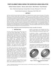
Flattening 3D Triangulations for Quality Surface Mesh Generation 137Fig. 6a. 2D domain of an automobile frame byWEFM at s=0.8 with boundary energy termFig. 6b. 2D triangular CSALF mesh onthe 2D domainFig. 6d. Layered mesh around frame cutoutFig. 6c. Corresponding final 3D meshFig. 6e. Boundary structured mesh aroundholeswhich has appreciable distortion but is not suitable for map meshing. Fig. 3b presentsa continuous section of a 2D domain developed by WFEM with s=1. This domain isregular and can be meshed by transfinite interpolation (mapped meshing) which is

138 K. Beatty and N. Mukherjeedepicted in Fig. 3c. Note, the domain has a small kink resulting from an irregular cutline chosen along the facet edges. The 3D mapped mesh reflects a small local distortionat that location.6.2 Accurate Transfinite Meshing NeedsTransfinite or mapped meshes are structured and mathematically accurate. The Coon’ssurface is not easily available on discrete geometry. Thus the efficiency and the accuracyof the flattening strategy is important for generating such meshes. Fig. 4a showsthe 2D domain of a pressure vessel wall surface developed by WFEM (s=0.0) with noboundary energy term. The corresponding 3D transfinite mesh is shown in Fig. 4b.When we zoom in on the elements near the vertical edge, as is evident in Fig. 4c, wenotice a lateral waviness in a certain region. This region corresponds to the two longitudinalkinks that exist on the vertical edges of the 2D domain. The wiggle factor of thetransfinite distortion parameter for this mesh is 0.12 which is far above the limitingvalue of 0.01. With a domain developed by WFEM (s = 0.3) with a boundary energyterm as pictured by Fig. 5a, these irregularities vanish and we get a perfect 3D transfinitemesh as shown in Fig. 5b-5c. The wiggle factor, described by eqn. (12) is 0.007.6.3 Boundary-Structured Free Meshing on Complex GeometryGood quality boundary-structured free meshes are important for a host of structuraland fluid flow analysis problems. Generation of such surface and volume meshes oncomplex industrial geometry is key to the success of an engineering design process.Fig. 6a shows the 2D domain of such a frame structure developed by WFEM (s=0.8).A triangular CSALF mesh is shown on the 2D domain in Fig. 6b. These zones are ofimportance to the designer as they are usually susceptible to high stresses. The final3D mesh shown in Fig. 6c reveals the same. It is important to note that the mesh, althoughunstructured in a global sense, is extremely layered/structured around all theinner circular/oval boundaries (see insets in Fig. 6d -6e).7 ConclusionIt was found the conformal (s=0) solution for the WEFM can be used for meshingprocesses based on a 2d domain. However, as in all conformal based solutions, thedimensions for non-developable triangulations are changed when they are mapped tothe UV domain. This can be a problem when high quality meshes are required. It wasfound an intermediate “altitude preserving” condition (s=1) of the WEFM, whichcompromises shape and dimension distortion, could give superior results when usedwith the presented map meshing process, and with forms of “mesh paving”. It wasfound that automatically choosing from all the valid solutions gave us the best overallstrategy. An automatically procedure for creating and evaluating constraints for repeatededges was developed. It was used to determine if each repeated edge should beleft free, treated as a scar, or be part of a periodic boundary condition. A boundaryenergy term in the WEFM formulation enabled the solution of indeterminate multiloopproblems, and generally improved the quality of the resulting domain. The differencein quality was readily apparent in the resulting 3D mapped mesh producedfrom the different domains.

Flattening 3D Triangulations for Quality Surface Mesh Generation 139References1. Floater, M.S., Hormann, K.: Surface parameterization: A tutorial and survey. In: Dodgson,M.S.E.N., Sabin, M. (eds.) Advances on Multiresolution in Geometric Modelling,Springer, Heidelberg (2004)2. Floater, M.S.: Mean value coordinates. Computer Aided Geometric Design 14(3), 231–250(1997)3. Hormann, K., Greiner, G.: MIPS: An Efficient Global Parameterization Method. In:Laurent, J.-P., Sablonniere, P., Schumaker, L.L. (eds.) Proceedings, Curve and SurfaceDesign, pp. 153–162. Vanderbilt University Press (2000)4. Levy, B., Petitjean, S., Ray, N., Maillot, J.: Least Squares Conformal Maps for AutomaticTexture Atlas Generation. In: Proceedings, ACM, SIGGRAPH (July 2002)5. Desbrun, M., Meyer, M., Alliez, P.: Intrinsic Parameterization of Surface Meshes. ComputerGraphics Forum (EUROGRAPHICS 2002) 21(3), 209–218 (2002)6. Sheffer, A., de Sturler, E.: Parameterization of faceted surfaces for meshing using anglebased flattening. Engineering with Computers 17, 326–337 (2001)7. Sheffer, A., Levy, B., Mogilnitsky, M., Bogomyakov, A.: ABF++: Fast and Robust AngleBased Flattening. Proceedings, ACM Transactions on Graphics 24(2), 311–330 (2005)8. Zayer, R., Levy, B. Seidel, H.-P.: Linear Angle Based Parameterization. In: Proceedings,Eurographics Symposium on Geometry Processing (2007)9. Gu, X., Yau, S.-T.: Global Conformal Surface Parameterization. In: Proceedings, EurographicsSymposium on Geometry Processing, pp. 127–137 (2003)10. Cabello, J.: Towards Quality Surface Meshing. In: Proceedings, 12th InternationalMeshing Roundtable, pp. 201–213 (2003)11. Schoof, A.J.G., Th, L.H., Van Beukering, M., Sluiter, M.L.C.: A general purpose twodimensionalmesh generator. Advances in Engineering Software 1(3), 131–136 (1979)12. Mukherjee, N.: CSALF: A combined subdivision and advancing loop-front approach togenerating controlled boundary structured free meshes. International Journal ofCAD/CAM (submitted, 2007)13. Perronnet, A.: Triangle, tetrahedron, pentahedron transfinite interpolations. Application tothe generation of C0 or G1-continuous algebraic meshes. In: Proceedings. InternationaConference of Numerical Grid Generation in Computational Field Simulations, Greenwich,England, July 6-9, 1998 vol. 7, pp. 467–476 (1998)14. Mukherjee, N.: High Quality Bi-Linear Transfinite Meshing with Interior Point Constraints.In: Pebay, P.P. (ed.) Proceedings, 15th International Meshing Roundtable, pp.309–323. Springer, Heidelberg (2006)15. Lo, S.H.: A New Mesh Generation Scheme For Arbitrary Planar Domains. InternationalJournal For Numerical Methods in Engineering (21), 1403–1426 (1985)