Linear Programming 1 An Introduction to Linear Programming

18.415/6.854 Advanced Algorithms October 1994Lecturer: Michel X. GoemansLinear Programming1 An Introduction to Linear ProgrammingLinear programming is a very important class of problems, both algorithmically andcombinatorially. Linear programming has many applications. From an algorithmicpoint-of-view, the simplex was proposed in the forties (soon after the war, and wasmotivated by military applications) and, although it has performed very well in practice,is known to run in exponential time in the worst-case. On the other hand, sincethe early seventies when the classes P and NP were defined, it was observed that linearprogramming is in NP∩ co-NP although no polynomial-time algorithm was known atthat time. The first polynomial-time algorithm, the ellipsoid algorithm, was only discoveredat the end of the seventies. Karmarkar’s algorithm in the mid-eighties lead tovery active research in the area of interior-point methods for linear programming. Weshall present one of the numerous variations of interior-point methods in class. Froma combinatorial perspective, systems of linear inequalities were already studied at theend of the last century by Farkas and Minkovsky. Linear programming, and especiallythe notion of duality, is very important as a proof technique. We shall illustrate itspower when discussing approximation algorithms. We shall also talk about networkflow algorithms where linear programming plays a crucial role both algorithmicallyand combinatorially. For a more in-depth coverage of linear programming, we referthe reader to [1, 4, 7, 8, 5].A linear program is the problem of optimizing a linear objective function in thedecision variables, x 1 ...x n , subject to linear equality or inequality constraints on thex i ’s. In standard form, it is expressed as:Minsubject to:n∑c j x j(objective function)j=1n∑a ij x j = b i , i =1...m (constraints)j=1x j ≥ 0, j =1...n (non-negativity constraints)where {a ij ,b i ,c j } are given.A linear program is expressed more conveniently using matrices:min c T x subject to{Ax = bx ≥ 0LP-1

wherex =b =c =A =⎛ ⎞x 1⎜ ⎟⎝ . ⎠ ∈ R n×1⎛x n ⎞b 1⎜ ⎟⎝ . ⎠ ∈ R m×1⎛b m⎞c 1⎜ ⎟⎝ . ⎠ ∈ R n×1c⎛ n ⎞a 11 ⎜ . ⎝ .. ⎟⎠ ∈ Rm×na mn2 Basic TerminologyDefinition 1 If x satisfies Ax = b, x ≥ 0, thenx is feasible.Definition 2 A linear program (LP) is feasible if there exists a feasible solution,otherwise it is said to be infeasible.Definition 3 An optimal solution x ∗ is a feasible solution s.t. c T x ∗ =min{c T x :Ax = b, x ≥ 0}.Definition 4 LP is unbounded (from below) if ∀λ ∈ R, ∃ afeasiblex ∗ s.t. c T x ∗ ≤ λ.3 Equivalent FormsA linear program can take on several forms. We might be maximizing instead ofminimizing. We might have a combination of equality and inequality contraints.Some variables may be restricted to be non-positive instead of non-negative, or beunrestricted in sign. Two forms are said to be equivalent if they have the same set ofoptimal solutions or are both infeasible or both unbounded.1. A maximization problem can be expressed as a minimization problem.max c T x ⇔ min −c T x2. An equality can be represented as a pair of inequalities.a T i x = b i⇔⇔{aTi x ≤ b ia T i x ≥ b{ iaTi x ≤ b i−a T i x ≤ −b iLP-2

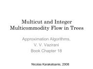
3. By adding a slack variable, an inequality can be represented as a combinationof equality and non-negativity constraints.a T i x ≤ b i ⇔ a T i x + s i = b i ,s i ≥ 0.4. Non-positivity constraints can be expressed as non-negativity constraints.To express x j ≤ 0, replace x j everywhere with −y j and impose the conditiony j ≥ 0.5. x may be unrestricted in sign.If x is unrestricted in sign, i.e. non-positive or non-negative, everywhre replacex j by x + j − x − j , adding the constraints x + j ,x − j ≥ 0.In general, an inequality can be represented using a combination of equality andnon-negativity constraints, and vice versa.Using these rules, min { c T x s.t. Ax ≥ b} can be transformed into min { c T x + − c T x −s.t. Ax + − Ax − − Is = b, x + ,x − ,s≥ 0}. The former LP is said to be in canonicalform, the latter in standard form.Conversely, an LP in standard form may be written in canonical form. min { c T xs.t. Ax = b, x ≥ 0} is equivalent to min { c T x s.t. Ax ≥ b, −Ax ≥−b, Ix ≥ 0}.⎛ ⎞⎛ ⎞This may be rewritten as A ′ x ≥ b ′ ,whereA ′ =⎜⎝A-AI⎟⎠ and b ′ =⎜⎝b-b0⎟⎠.4 ExampleConsider the following linear program:min x 2 subject to⎧⎪⎨⎪⎩x 1 ≥ 23x 1 − x 2 ≥ 0x 1 + x 2 ≥ 6−x 1 + 2x 2 ≥ 0The optimal solution is (4, 2) of cost 2 (see Figure 1). If we were maximizing x 2instead of minimizing under the same feasible region, the resulting linear programwould be unbounded since x 2 can increase arbitrarily. From this picture, the readershould be convinced that, for any objective function for which the linear program isbounded, there exists an optimal solution which is a “corner” of the feasible region.We shall formalize this notion in the next section.LP-3

3x − x > 01 2x2(2,4)−x + 2x > 012(2,1)x > 21x + x > 612x1Figure 1: Graph representing primal in example.An example of an infeasible linear program can be obtained by reversing some ofthe inequalities of the above LP:5 The Geometry of LPLet P = {x : Ax = b, x ≥ 0} ⊆R n .x 1 ≤ 23x 1 − x 2 ≥ 0x 1 + x 2 ≥ 6−x 1 + 2x 2 ≤ 0.Definition 5 x is a vertex of P if ̸ ∃y ≠0s.t. x + y, x − y ∈ P .Theorem 1 Assume min{c T x : x ∈ P } is finite, then ∀x ∈ P, ∃ a vertex x ′c T x ′ ≤ c T x.such thatProof:If x is a vertex, then take x ′ = x.If x is not a vertex, then, by definition, ∃y ≠0s.t. x + y, x − y ∈ P . SinceA(x + y) =b and A(x − y) =b, Ay =0.LP-4

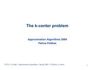
WLOG, assume c T y ≤ 0 (take either y or −y). If c T y =0,choosey such that ∃js.t. y j < 0. Since y ≠0andc T y = c T (−y) = 0, this must be true for either y or −y.Consider x + λy, λ > 0. c T (x + λy) =c T x + λc T y ≤ c T x,sincec T y is assumednon-positive.Case 1 ∃j such that y j < 0As λ increases, component j decreases until x + λy is no longer feasible.Choose λ =min {j:yj

x2(0,1)(0,0) x1Figure 2: A polyhedron with no vertex.Theorem 4 Let P = {x : Ax = b, x ≥ 0}. For x ∈ P ,letA x be a submatrix of Acorresponding to j s.t. x j > 0. Then x is a vertex iff A x has linearly independentcolumns. (i.e. A x has full column rank.)Example A =Proof:⎡⎢⎣2 1 3 07 3 2 10 0 0 5⎤⎥⎦ x =⎡⎢⎣2010⎤⎡⎥⎦ A ⎢x = ⎣2 37 20 0⎤⎥⎦, andx is a vertex.Show ¬i →¬ii.Assume x is not a vertex. Then, by definition, ∃y ≠0s.t. x + y, x − y ∈ P .Let A y be submatrix corresponding to non-zero components of y.As in the proof of Theorem 1,}Ax + Ay = b⇒ Ay =0.Ax − Ay = bTherefore, A y has dependent columns since y ≠0.Moreover,}x + y ≥ 0⇒ yx − y ≥ 0 j = 0 whenever x j =0.Therefore A y is a submatrix of A x . Since A y is a submatrix of A x , A x haslinearly dependent columns.LP-6

Show ¬ii →¬i.Suppose A x has linearly dependent columns. Then ∃y s.t. A x y =0,y ≠0.Extend y to R n by adding 0 components. Then ∃y ∈ R n s.t. Ay =0, y ≠0and y j = 0 wherever x j =0.Consider y ′ = λy for small λ ≥ 0. Claim that x + y ′ ,x− y ′ ∈ P ,byargumentanalogous to that in Case 1 of the proof of Theorem 1, above. Hence, x is nota vertex.✷6 BasesLet x be a vertex of P = {x : Ax = b, x ≥ 0}. Suppose first that |{j : x j > 0}| = m(where A is m × n). In this case we denote B = {j : x j > 0}. AlsoletA B = A x ;weuse this notation not only for A and B, but also for x and for other sets of indices.Then A B is a square matrix whose columns are linearly independent (by Theorem4), so it is non-singular. Therefore we can express x as x j =0ifj ∉ B, and sinceA B x B = b, it follows that x B = A −1B b. The variables corresponding to B will be calledbasic. The others will be referred to as nonbasic. The set of indices corresponding tononbasic variables is denoted by N = {1,... ,n}−B. Thus, we can write the aboveas x B = A −1B b and x N =0.Without loss of generality we will assume that A has full row rank, rank(A) =m.Otherwise either there is a redundant constraint in the system Ax = b (and we canremove it), or the system has no solution at all.If |{j : x j > 0}| 0} indifferent ways). A basis might not lead to any basic feasible solution since A −1B b isnot necessarily nonnegative.LP-7

Example:x 1 + x 2 + x 3 =52x 1 − x 2 +2x 3 =1x 1 ,x 2 ,x 3 ≥ 0We can select as a basis B = {1, 2}. Thus,N = {3} andA B =A −1B =( )1 12 −1)( 132313−13)A −1B b = (23x = (2, 3, 0)Remark. A crude upper bound on the number of vertices of P is ( )nm . This numberis exponential (it is upper bounded by n m ). We can come up with a tighter approximationof ( )n− m 2m , though this is still exponential. Thereasonwhythenumberis2much smaller is that most basic solutions to the system Ax = b (which we counted)are not feasible, that is, they do not satisfy x ≥ 0.7 The Simplex MethodThe Simplex algorithm [Dantzig,1947] [2] solves linear programming problems byfocusing on basic feasible solutions. The basic idea is to start from some vertex v andlook at the adjacent vertices. If an improvement in cost is possible by moving to oneof the adjacent vertices, then we do so. Thus, we will start with a bfs correspondingtoabasisB and, at each iteration, try to improve the cost of the solution by removingone variable from the basis and replacing it by another.We begin the Simplex algorithm by first rewriting our LP in the form:mins.t.c B x B + c N x NA B x B + A N x N = bx B ,x N ≥ 0Here B is the basis corresponding to the bfs we are starting from. Note that, forany solution x, x B = A −1B b − A −1B A N x N and that its total cost, c T x can be specifiedas follows:LP-8

c T x = c B x B + c N x N= c B (A −1B b − A−1 B A Nx N )+c N x N= c B A −1B b +(c N − c B A −1B A N)x NWe denote the reduced cost of the non-basic variables by ˜c N ,˜c N = c N − c B A −1B A N ,i.e. the quantity which is the coefficient of x N above. If there is a j ∈ N such that˜c j < 0, then by increasing x j (up from zero) we will decrease the cost (the value ofthe objective function). Of course x B depends on x N , and we can increase x j only aslong as all the components of x B remain positive.So in a step of the Simplex method, we find a j ∈ N such that ˜c j < 0, and increaseit as much as possible while keeping x B ≥ 0. It is not possible any more to increasex j , when one of the components of x B is zero. What happened is that a non-basicvariable is now positive and we include it in the basis, and one variable which wasbasic is now zero, so we remove it from the basis.If, on the other hand, there is no j ∈ N such that ˜c j < 0, then we stop, andthe current basic feasible solution is an optimal solution. This follows from the newexpression for c T x since x N is nonnegative.Remarks:1. Note that some of the basic variables may be zero to begin with, and in thiscase it is possible that we cannot increase x j at all. In this case we can replacesay j by k in the basis, but without moving from the vertex corresponding tothe basis. In the next step we might replace k by j, and be stuck in a loop.Thus, we need to specify a “pivoting rule” to determine which index shouldenter the basis, and which index should be removed from the basis.2. While many pivoting rules (including those that are used in practice) can leadto infinite loops, there is a pivoting rule which will not (known as the minimalindex rule - choose the minimal j and k possible [Bland, 1977]). This fact wasdiscovered by Bland in 1977. There are other methods of “breaking ties” whicheliminate infinite loops.3. There is no known pivoting rule for which the number of pivots in the worstcase is better than exponential.4. The question of the complexity of the Simplex algorithm and the last remarkleads to the question of what is the length of the shortest path between twovertices of a convex polyhedron, where the path is along edges, and the lengthof the path in measured in terms of the number of vertices visited.LP-9

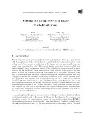
Hirsch Conjecture: For m hyperplanes in d dimensions the length of theshortest path between any two vertices of the arrangement is at most m − d.This is a very open question — there is not even a polynomial bound provenon this length.On the other hand, one should note that even if the Hirsch Conjecture is true,it doesn’t say much about the Simplex Algorithm, because Simplex generatespaths which are monotone with respect to the objective function, whereas theshortest path need not be monotone.Recently, Kalai (and others) has considered a randomized pivoting rule. Theidea is to randomly permute the index columns of A and to apply the Simplexmethod, always choosing the smallest j possible. In this way, it is possible toshow a subexponential bound on the expected number of pivots. This leads toa subexponential bound for the diameter of any convex polytope defined by mhyperplanes in a d dimension space.The question of the existence of a polynomial pivoting scheme is still openthough. We will see later a completely different algorithm which is polynomial,although not strongly polynomial (the existence of a strongly polynomial algorithmfor linear programming is also open). That algorithm will not move fromone vertex of the feasible domain to another like the Simplex, but will confineits interest to points in the interior of the feasible domain.A visualization of the geometry of the Simplex algorithm can be obtained fromconsidering the algorithm in 3 dimensions (see Figure 3). For a problem in the formmin{c T x : Ax ≤ b} the feasible domain is a polyhedron in R 3 , and the algorithmmoves from vertex to vertex in each step (or does not move at all).8 When is a Linear Program Feasible ?We now turn to another question which will lead us to important properties of linearprogramming. Let us begin with some examples.We consider linear programs of the form Ax = b, x ≥ 0. As the objective functionhas no effect on the feasibility of the program, we ignore it.We first restrict our attention to systems of equations (i.e. we neglect the nonnegativityconstraints).Example: Consider the system of equations:x 1 + x 2 + x 3 = 62x 1 + 3x 2 + x 3 = 82x 1 + x 2 + 3x 3 = 0and the linear combinationLP-10

ObjectivefunctionFigure 3: Traversing the vertices of a convex body (here a polyhedron in R 3 ).−4 × x 1 + x 2 + x 3 = 61 × 2x 1 + 3x 2 + x 3 = 81 × 2x 1 + x 2 + 3x 3 = 0The linear combination results in the equation0x 1 +0x 2 +0x 3 = −16which means of course that the system of equations has no feasible solution.In fact, an elementary theorem of linear algebra says that if a system has nosolution, there is always a vector y such as in our example (y =(−4, 1, 1)) whichproves that the system has no solution.Theorem 5 Exactly one of the following is true for the system Ax = b:1. There is x such that Ax = b.2. There is y such that A T y =0but y T b =1.This is not quite enough for our purposes, because a system can be feasible,but still have no non-negative solutions x ≥ 0. Fortunately, the following lemmaestablishes the equivalent results for our system Ax = b, x ≥ 0.Theorem 6 (Farkas’ Lemma) Exactly one of the following is true for the systemAx = b, x ≥ 0:LP-11

1. There is x such that Ax = b, x ≥ 0.2. There is y such that A T y ≥ 0 but b T y

zpbFigure 5: The Projection Theorem.Since p ∈ K, thereisaw ≥ 0 such that Aw = p. According to the ProjectionTheorem, for all z ∈ K, (z − p) T (b − p) ≤ 0Thatis,forallx ≥ 0(Ax − p) T (b − p) ≤ 0We define y = p−b, which implies (Ax−p) T y ≥ 0. Since Aw = p, (Ax−Aw) T y ≥0. (x − w) T (A T y) ≥ 0 for all x ≥ 0 (remember that w wasfixedbychoosingb).⎛ ⎞0Set x = w +0.(w plus a unit vector with a 1 in the i-th row). Note that x⎜ ⎟⎝1. ⎠0is non-negative, because w ≥ 0.This will extract the i-th column of A, so we conclude that the i-th component ofA T y is non-negative (A T y) i ≥ 0, and since this is true for all i, A T y ≥ 0.Now it only remains to show that y T b0. So y T b = p T y −y T y

The intuition behind the precise form for 2. in the previous theorem lies in the proofthat both cannot happen. The contradiction 0 = 0x =(y T A)x = y T (Ax) =y T b

Example:z =min x 1 + 2x 2 + 4x 3x 1 + x 2 + 2x 3 = 52x 1 + x 2 + 3x 3 = 8The first equality gives a lower bound of 5 on the optimum value z, sincex 1 +2x 2 +4x 3 ≥ x 1 + x 2 +2x 3 = 5 because of nonnegativity of the x i . We can get an evenbetter lower bound by taking 3 times the first equality minus the second one. Thisgives x 1 +2x 2 +3x 3 =7≤ x 1 +2x 2 +4x 3 , implying a lower bound of 7 on z. Forx =⎛⎜⎝320⎞⎟⎠, the objective function is precisely 7, implying optimality. The mechanismof generating lower bounds is formalized by the dual linear program:max 5y 1 + 8y 2y 1 + 2y 2 ≤ 1y 1 + y 2 ≤ 22y 1 + 3y 2 ≤ 4y 1 represents the multiplier for the first constraint and y 2 the multiplier for the secondconstraint, ( ) This LP’s objective function also achieves a maximum value of 7 at y =3.−1We now formalize the notion of duality. Let P and D be the following pair of duallinear programs:(P ) z =min{c T x : Ax = b, x ≥ 0}(D) w =max{b T y : A T y ≤ c}.(P ) is called the primal linear program and (D) thedual linear program.In the proof below, we show that the dual of the dual is the primal. In otherwords, if one formulates (D) as a linear program in standard form (i.e. in the sameform as (P )), its dual D(D) can be seen to be equivalent to the original primal (P ).In any statement, we may thus replace the roles of primal and dual without affectingthe statement.Proof:The dual problem D is equivalent to min{−b T y : A T y + Is = c, s ≥ 0}. Changingforms we get min{−b T y + +b T y − : A T y + −A T y − +Is = c, and y + ,y − ,s≥ 0}. Takingthe dual of this we obtain: max{−c T x : A(−x) ≤−b, −A(−x) ≤ b, I(−x) ≤ 0}. Butthis is the same as min{c T x : Ax = b, x ≥ 0} and we are done.✷We have the following results relating w and z.Lemma 9 (Weak Duality) z ≥ w.LP-15

Proof:Suppose x is primal feasible and y is dual feasible. Then, c T x ≥ y T Ax = y T b,thus z =min{c T x : Ax = b, x ≥ 0} ≥max{b T y : A T y ≤ c} = w.✷From the preceding lemma we conclude that the following cases are not possible(these are dual statements):1. P is feasible and unbounded and D feasible.2. P is feasible and D is feasible and unbounded.We should point out however that both the primal and the dual might be infeasible.To prove a stronger version of the weak duality lemma, let’s recall the followingcorollary of Farkas’ Lemma (Theorem 8):Corollary 10 Exactly one of the following is true:1. ∃x ′ : A ′ x ′ ≤ b ′ .2. ∃y ′ ≥ 0:(A ′ ) T y ′ =0and (b ′ ) T y ′ < 0.Theorem 11 (Strong Duality) If P or D is feasible then z = w.Proof:We only need to show that z ≤ w. Assume without loss of generality (by duality)that P is feasible. If P is unbounded, then by Weak Duality, wehavethatz = w =−∞. Suppose P is bounded, and let x ∗ be an optimal solution, i.e. Ax ∗ = b, x ∗ ≥ 0and c T x ∗ = z. We claim that ∃y s.t. A T y ≤ c and b T y ≥ z. If so we are done.Suppose no such y exists. Then, by the preceding corollary, with A ′ =( )( )cxb ′ = , x−z′ = y, y ′ = , ∃x ≥ 0, λ ≥ 0 such thatλ(AT−b T ),andAx = λbc T x

9.1 Rules for Taking Dual ProblemsIf P is a minimization problem then D is a maximization problem. If P is a maximizationproblem then D is a minimization problem. In general, using the rules fortransforming a linear program into standard form, we have that the dual of (P ):z =minc T 1 x 1 + c T 2 x 2 + c T 3 x 3s.t.A 11 x 1 + A 12 x 2 + A 13 x 3 = b 1A 21 x 1 + A 22 x 2 + A 23 x 3 ≥ b 2A 31 x 1 + A 32 x 2 + A 33 x 3 ≤ b 3x 1 ≥ 0 ,x 2 ≤ 0 ,x 3 UIS(where UIS means “unrestricted in sign” to emphasize that no constraint is on thevariable) is (D)w =maxb T 1 y 1 + b T 2 y 2 + b T 3 y 3s.t.A T 11 y 1 + A T 21 y 2 + A T 31 y 3 ≤ c 1A T 12y 1 + A T 22y 2 + A T 32y 3 ≥ c 2A T 13y 1 + A T 23y 2 + A T 33y 3 = c 3y 1 UIS ,y 2 ≥ 0 ,y 3 ≤ 010 Complementary SlacknessLet P and D be(P ) z =min{c T x : Ax = b, x ≥ 0}(D) w =max{b T y : A T y ≤ c},and let x be feasible in P ,andy be fesible in D. Then, by weak duality, we know thatc T x ≥ b T y. We call the difference c T x − b T y the duality gap. Then we have that theduality gap is zero iff x is optimal in P ,andy is optimal in D. That is, the dualitygap can serve as a good measure of how close a feasible x and y are to the optimalsolutions for P and D. The duality gap will be used in the description of the interiorpoint method to monitor the progress towards optimality.It is convenient to write the dual of a linear program as(D) w =max{b T y : A T y + s = c for some s ≥ 0}Then we can write the duality gap as follows:c T x − b T y = c T x − x T A T y= x T (c − A T y)= x T sLP-17

since A T y + s = c.The following theorem allows to check optimality of a primal and/or a dual solution.Theorem 12 (Complementary Slackness)Let x ∗ , (y ∗ ,s ∗ ) be feasible for (P ), (D) respectively. The following are equivalent:1. x ∗ is an optimal solution to (P ) and (y ∗ ,s ∗ ) is an optimal solution to (D).2. (s ∗ ) T x ∗ =0.3. x ∗ js ∗ j =0, ∀ j =1,... ,n.4. If s ∗ j > 0 then x ∗ j =0.Proof:Suppose (1) holds, then, by strong duality, c T x ∗ = b T y ∗ .Sincec = A T y ∗ + s ∗ andAx ∗ = b, wegetthat(y ∗ ) T Ax ∗ +(s ∗ ) T x ∗ =(x ∗ ) T A T y ∗ , and thus, (s ∗ ) T x ∗ = 0 (i.e (2)holds). It follows, since x ∗ j , s∗ j ≥ 0, that x∗ j s∗ j =0,∀ j =1,... ,n (i.e. (3) holds).Hence, if s ∗ j > 0thenx∗ j =0,∀ j =1,... ,n (i.e. (4) holds). The converse also holds,and thus the proof is complete.✷In the example of section 9, the complementary slackness equations correspondingto the primal solution x =(3, 2, 0) T would be:y 1 +2y 2 =1y 1 + y 2 =2Note that this implies that y 1 =3andy 2 = −1. Since this solution satisfies theother constraint of the dual, y is dual feasible, proving that x is an optimum solutionto the primal (and therefore y is an optimum solution to the dual).11 Size of a Linear Program11.1 Size of the InputIf we want to solve a Linear Program in polynomial time, we need to know whatwould that mean, i.e. what would the size of the input be. To this end we introducetwo notions of the size of the input with respect to which the algorithm we presentwill run in polynomial time. The first measure of the input size will be the size ofa LP, but we will introduce a new measure L of a LP that will be easier to workwith. Moreover, we have that L ≤ size(LP ), so that any algorithm running in timepolynomial in L will also run in time polynomial in size(LP).LP-18

Let’s consider the linear program of the form:min c T xs.t.Ax = bx ≥ 0where we are given as inputs the coefficients of A (an m × n matrix), b (an m × 1vector), and c (an n × 1 vector), whith rationial entries.We can further assume, without loss of generality, that the given coefficients areall integers, since any LP with rational coefficients can be easily transformed into anequivalent one with integer coefficients (just multiply everything by l.c.d.). In therest of these notes, we assume that A, b, c have integer coefficients.For any integer n, we define its size as follows:size(n) △ =1+⌈log 2 (|n| +1)⌉where the first 1 stands for the fact that we need one bit to store the sign of n, size(n)represents the number of bits needed to encode n in binary. Analogously, we definethe size of a p × 1 vector d, andofap × l matrix M as follows:size(v) = △ ∑ pi=1 size(v i )size(M) = △ ∑ p ∑ lj=1i=1 size(m ij )We are then ready to talk about the size of a LP.Definition 6 (Size of a linear program)size(LP) △ =size(A)+size(b)+size(c).A more convenient definition of the size of a linear program is given next.Definition 7whereL △ =size(detmax)+size(bmax)+size(cmax)+m + ndetmaxbmaxcmax△= max(| det(A ′ )|)A ′△= max(|b i |)i△= maxj(|c j |)and A ′ is any square submatrix of A.LP-19

Proposition 13 L

11.2 Size of the OutputIn order to even hope to solve a linear program in polynomial time, we better makesure that the solution is representable in size polynomial in L. We know already thatif the LP is feasible, there is at least one vertex which is an optimal solution. Thus,when finding an optimal solution to the LP, it makes sense to restrict our attentionto vertices only. The following theorem makes sure that vertices have a compactrepresentation.Theorem 15 Let x be a vertex of the polyhedron defined by Ax = b, x ≥ 0. Then,( )x T p1 p 2=q q ...p n,qwhere p i (i =1,... ,n), q∈ N,and0 ≤ p i < 2 L1 ≤ q

Theorem 16 LP ∈ NP ∩ co-NPProof:First, we prove that LP ∈ NP.If the linear program is feasible and bounded, the “certificate” for verification ofinstances for which min{c T x : Ax = b, x ≥ 0} ≤λ is a vertex x ′ of {Ax = b, x ≥ 0}s.t. c T x ′ ≤ λ. This vertex x ′ always exists since by assumption the minimum is finite.Given x ′ , it is easy to check in polynomial time whether Ax ′ = b and x ′ ≥ 0. We alsoneed to show that the size of such a certificate is polynomially bounded by the sizeof the input. This was shown in section 11.2.If the linear program is feasible and unbounded, then, by strong duality, the dualis infeasible. Using Farkas’ lemma on the dual, we obtain the existence of ˜x: A˜x =0,˜x ≥ 0andc T ˜x = −1 < 0. Our certificate in this case consists of both a vertex of{Ax = b, x ≥ 0} (to show feasiblity) and a vertex of {Ax =0,x ≥ 0, c T x = −1}(to show unboundedness if feasible). By choosing a vertex x ′ of {Ax =0,x ≥ 0,c T x = −1}, we insure that x ′ has polynomial size (again, see Section 11.2).This proves that LP ∈ NP. (Notice that when the linear program is infeasible,the answer to LP is “no”, but we are not responsible to offer such an answer in orderto show LP ∈ NP).Secondly, we show that LP ∈ co-NP, i.e. LP ∈ NP, where LP is defined as:Input: A, b, c, and a rational number λ,Question: Is min{c T x : Ax = b, x ≥ 0} >λ?If {x : Ax = b, x ≥ 0} is nonempty, we can use strong duality to show that LP isindeed equivalent to:Input: A, b, c, and a rational number λ,Question: Is max{b T y : A T y ≤ c} >λ?which is also in NP, for the same reason as LP is.If the primal is infeasible, by Farkas’ lemma we know the existence of a y s.t.A T y ≥ 0andb T y = −1 < 0. This completes the proof of the theorem.✷13 Solving a Liner Program in Polynomial TimeThe first polynomial-time algorithm for linear programming is the so-called ellipsoidalgorithm which was proposed by Khachian in 1979 [6]. The ellipsoid algorithm was infact first developed for convex programming (of which linear programming is a specialcase) in a series of papers by the russian mathematicians A.Ju. Levin and, D.B. Judinand A.S. Nemirovskii, and is related to work of N.Z. Shor. Though of polynomialrunning time, the algorithm is impractical for linear programming. Nevertheless ithas extensive theoretical applications in combinatorial optimization. For example,the stable set problem on the so-called perfect graphs can be solved in polynomialtime using the ellipsoid algorithm. This is however a non-trivial non-combinatorialalgorithm.LP-22

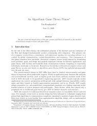
In 1984, Karmarkar presented another polynomial-time algorithm for linear programming.His algorithm avoids the combinatorial complexity (inherent in the simplexalgorithm) of the vertices, edges and faces of the polyhedron by staying wellinside the polyhedron (see Figure 13). His algorithm lead to many other algorithmsfor linear programming based on similar ideas. These algorithms are known as interiorpoint methods.Figure 6: Exploring the interior of a convex body.It still remains an open question whether there exists a strongly polynomial algorithmfor linear programming, i.e. an algorithm whose running time depends on mand n and not on the size of any of the entries of A, b or c.In the rest of these notes, we discuss an interior-point method for linear programmingand show its polynomiality.High-level description of an interior-point algorithm:1. If x (current solution) is close to the boundary, then map the polyhedron ontoanother one s.t. x is well in the interior of the new polyhedron (see Figure 7).2. Make a step in the transformed space.3. Repeat (a) and(b) until we are close enough to an optimal solution.Before we give description of the algorithm we give a theorem, the corollary ofwhich will be a key tool used in determinig when we have reached an optimal solution.LP-23

Theorem 17 Let x 1 ,x 2 be vertices of Ax = b,x ≥ 0.If c T x 1 ≠ c T x 2 then |c T x 1 − c T x 2 | > 2 −2L .Proof:By Theorem 15, ∃ q i , q 2 , such that 1 ≤ q 1 ,q 2 < 2 L ,andq 1 x 1 ,q 2 x 2 ∈ N n . Furthermore,|c T x 1 − c T x 2 | ==∣∣q 1 c T x 1− q 2c T ∣x ∣∣∣∣ 2q 1 q 2q 1 q 2 (c T x 1 − c T x 2 )q 1 q 2∣ ∣∣∣∣≥ 1 since c T x 1 − c T x 2 ≠0,q 1 ,q 2 ≥ 1q 1 q 21>2 L 2 L =2−2L since q 1 ,q 2 < 2 L .Corollary 18 Assume z =min{c T x : Ax = b, x ≥ 0}.} {{ }polyhedron PAssume x is feasible to P , and such that c T x ≤ z +2 −2L .Then, any vertex x ′ such that c T x ′ ≤ c T x is an optimal solution of the LP.Proof:Suppose x ′ is not optimal. Then, ∃x ∗ , an optimal vertex, such that c T x ∗ = z.Since x ′ is not optimal, c T x ′ ≠ c T x ∗ ,andbyTheorem17⇒ c T x ′ − c T x ∗ > 2 −2L⇒ c T x ′ > c T x ∗ +2 −2L= Z +2 −2L≥ c T x by definition of x≥ c T x ′ by definition of x ′⇒ c T x ′ > c T x ′ ,a contradiction.✷What this corollary tells us is that we do not need to be very precise when choosingan optimal vertex. More precisely we only need to compute the objective functionwith error less than 2 −2L . If we find a vertex that is within that margin of error, thenit will be optimal.LP-24✷

xx’PP’Figure 7: A centering mapping. If x is close to the boundary, we map the polyhedronP onto another one P ′ , s.t. the image x ′ of x is closer to the center of P ′ .13.1 Ye’s Interior Point AlgorithmIn the rest of these notes we present Ye’s [9] interior point algorithm for linear programming.Ye’s algorithm (among several others) achieves the best known asymptoticrunning time in the literature, and our presentation incorporates some simplificationsmade by Freund [3].We are going to consider the following linear programming problem:⎧⎪⎨ minimize Z = c T x(P ) subject to Ax = b,⎪⎩x ≥ 0and its dual⎧⎪⎨ maximize W = b T y(D) subject to A T y + s = c,⎪⎩s ≥ 0.The algorithm is primal-dual, meaning that it simultaneously solves both theprimal and dual problems. It keeps track of a primal solution x and a vector of dualslacks s (i.e. ∃ y : A T y = c − s) such that x>0ands>0. The basic idea of thisalgorithm is to stay away from the boundaries of the polyhedron (the hyperplanesx j ≥ 0ands j ≥ 0, j =1, 2,... ,n) while approaching optimality. In other words, wewant to make the duality gapc T x − b T y = x T s>0LP-25

very small but stay away from the boundaries. Two tools will be used to achieve thisgoal in polynomial time.Tool 1: Scaling (see Figure 7)Scaling is a crucial ingredient in interior point methods. The two types of scalingcommonly used are projective scaling (the one used by Karmarkar) and affine scaling(the one we are going to use).Suppose the current iterate is x>0ands>0, where x =(x 1 , x 2 ,... ,x n ) T ,thentheaffinescalingmapsx to x ′ as follows.⎛ ⎞⎛x 1x 2x =..−→ x ′ =⎜ ⎟⎝ . ⎠⎜⎝x nNotice this transformation maps x to e =(1,... ,1) T .We can express the scaling transformation in matrix form as x ′ = X −1 x or x =Xx ′ ,where⎛⎞x 1 0 0 ... 00 x 2 0 ... 0X =. . .⎜⎝ 0 0 ... x n−1 0⎟⎠0 0 ... 0 x n.Using matrix notation we can rewrite the linear program (P) in terms of the transformedvariables as:minimize Z = c T Xx ′subject to AXx ′ = b,x ′ ≥ 0.If we define c = Xc (note that X = X T )andA = AX we can get a linear programin the original form as follows.minimize Z = c T x ′subject to Ax ′ = b,x ′ ≥ 0.We can also write the dual problem (D) as:x 1x 1x 2x 2...x nx n⎞⎟⎠maximize W = b T ysubject to (AX) T y + Xs = c,LP-26Xs ≥ 0.

or, equivalently,maximize W = b T ysubject to A T y + s ′ = c,s ′ ≥ 0where s ′ = Xs, i.e.Onecaneasilyseethat⎛s ′ =⎜⎝⎞s 1 x 1s 2 x 2.⎟. ⎠s n x n.x j s j = x ′ j s′ j ∀j ∈{1,... ,n} (3)and, therefore, the duality gap x T s = ∑ j x j s j remains unchanged under affine scaling.As a consequence, we will see later that one can always work equivalently in thetransformed space.Tool 2: Potential FunctionOur potential function is designed to measure how small the duality gap is andhow far the current iterate is away from the boundaries. In fact we are going to usethe following “logarithmic barrier function”.Definition 9 (Potential Function, G(x, s))n∑G(x, s) = △ q ln(x T s) − ln(x j s j ), for some q,j=1where q is a parameter that must be chosen appropriately.Note that the first term goes to −∞ as the duality gap tends to 0, and the secondterm goes to +∞ as x i → 0ors i → 0forsomei. Two questions arise immediatelyconcerning this potential function.Question 1: How do we choose q?Lemma 19 Let x, s > 0 be vectors in R n×1 .Thenn∑n ln x T s − ln x j s j ≥ n ln n.j=1LP-27

Proof:Given any n positive numbers t 1 ,... ,t n , we know that their geometric mean doesnot exceed their arithmetic mean, i.e.⎛ ⎞1/n⎛n∏⎝ t j⎠ ≤ 1 ⎝j=1nn∑j=1t j⎞⎠Taking the logarithms of both sides we have⎛ ⎞ ⎛ ⎞1n∑n∑⎝ ln t j⎠ ≤ ln ⎝ t j⎠ − ln n.nj=1j=1Rearranging this inequality we get⎛ ⎞ ⎛n∑n∑n ln ⎝ t j⎠ − ⎝j=1j=1ln t j⎞⎠ ≥ n ln n.(In fact the last inequality can be derived directly from the concavity of the logarithmicfunction). The lemma follows if we set t j = x j s j .✷Since our objective is that G →−∞as x T s → 0 (since our primary goal is to getclose to optimality), according to Lemma 19, we should choose some q>n(noticethat ln x T s →−∞as x T s → 0) . In particular, if we choose q = n + 1, the algorithmwill terminate after O(nL) iterations. In fact we are going to set q = n + √ n,whichgives us the smallest number — O( √ nL) — of iterations by this method.Question 2: When can we stop?Suppose that x T s ≤ 2 −2L ,thenc T x − Z ≤ c T x − b T y = x T s ≤ 2 −2L ,whereZ isthe optimum value to the primal problem. From Corollary 18, the following claimfollows immediately.Claim 20 If x T s ≤ 2 −2L , then any vertex x ∗ satisfying c T x ∗ ≤ c T x is optimal.In order to find x ∗ from x, two methods can be used. One is based on purelyalgebraic techniques (but is a bit cumbersome to describe), while the other (thecleanest one in literature) is based upon basis reduction for lattices. We shall notelaborate on this topic, although we’ll get back to this issue when discussing basisreduction in lattices.Lemma 21 Let x, s be feasible primal-dual vectors such that G(x, s) ≤−k √ nL forsome constant k. Thenx T s

Proof:By the definition of G(x, s) and the previous theorem we have:Rearranging we obtain−k √ nL ≥ G(x, s)= (n + √ n∑n)lnx T s − ln x j s jj=1≥ √ n ln x T s + n ln n.ln x T s ≤ −kL − √ n ln n< −kL.Thereforex T s 0, s 0 > 0, and y 0 such that Ax 0 = b, A T y 0 + s 0 = c and G(x 0 ,s 0 )=O( √ nL). (Details are not covered in class but can be found in the appendix. Thegeneral idea is as follows. By augmenting the linear program with additional variables,it is easy to obtain a feasible solution. Moreover, by carefully choosing the augmentedlinear program, it is possible to have feasible primal and dual solutions x and s suchthat all x j ’s and s j ’s are large (say 2 L ). This can be seen to result in a potential ofO( √ nL).)Iteration:while G(x i ,s i ) > −2 √ nL⎧⎪⎨ either a primal step (changing x i }only)do or a dual step (changing s i to get (xonly)i+1 ,s i+1 )⎪⎩i := i +1The iterative step is as follows. Affine scaling maps (x i ,s i )to(e, s ′ ). In thistransformed space, the point is far away from the boundaries. Either a dual orLP-29

a a g1 2g−ddNull space of A{x: Ax = 0}Figure 8: Null space of A and gradient direction g.primal step occurs, giving (˜x, ˜s) and reducing the potential function. The point isthen mapped back to the original space, resulting in (x i+1 ,s i+1 ).Next, we are going to describe precisely how the primal or dual step is made suchthatG(x i+1 ,s i+1 ) − G(x i ,s i ) ≤− 7120 < 0holds for either a primal or dual step, yielding an O( √ nL) total number of iterations.In order to find the new point (˜x, ˜s) given the current iterate (e, s ′ ) (rememberwe are working in the transformed space), we compute the gradient of the potentialfunction. This is the direction along which the value of the potential function changesat the highest rate. Let g denote the gradient. Recall that (e, s ′ ) is the map of thecurrent iterate, we obtaing = ∇ x G(x, s)| (e,s ′ )⎛ ⎞= q 1/x 1x T s s − ⎜ ⎟⎝ . ⎠∣1/x n=∣ (e,s ′ )qe T s ′ s′ − e (4)We would like to maximize the change in G, so we would like to move in thedirection of −g. However, we must insure the new point is still feasible (i.e. A˜x = b).Let d be the projection of g onto the null space {x : Ax =0} of A. Thus, we willmove in the direction of −d.Claim 22 d =(I − A(A A T ) −1 A)g.LP-30

Proof:Since g − d is orthogonal to the null space of A, it must be the combination ofsome row vectors of A. Hence we have{ Ad =0∃w, s.t. A T w = g − d.This implies⎧⎨⎩A T w = g − d(A A T )w = Ag(normal equations).andSolving the normal equations, we getw =(A A T ) −1 Agd = g − A T (A A T ) −1 Ag =(I − A T (A A T ) −1 A)g.✷A potential problem arises if g is nearly perpendicular to the null space of A. Inthis case, ||d|| will be very small, and each primal step will not reduce the potentialgreatly. Instead, we will perform a dual step.In particular, if ||d|| = ||d|| 2 = √ d T d ≥ 0.4, we make a primal step as follows.Claim 23 ˜x >0.˜x = e − 14||d|| d˜s = s ′ .Proof:˜x j =1− 1 d j≥ 3 > 0.✷4 ||d|| 4This claim insures that the new iterate is still an interior point. For the similarreason, we will see that ˜s >0 when we make a dual step.Proposition 24 Whenaprimalstepismade,G(˜x, ˜s) − G(e, s ′ ) ≤− 7120 .If ||d|| < 0.4, we make a dual step. Again, we calculate the gradienth = ∇ s G(x, s)| (e,s ′ )⎛1/s ′ ⎞1q=e T s e − ⎜ ⎟′ ⎝ . ⎠ (5)1/s ′ nLP-31

Notice that h j = g j /s j ,thush and g can be seen to be approximately in the samedirection.Suppose the current dual feasible solution is y ′ ,s ′ such thatA T y ′ + s ′ = c.Again, we restrict the solution to be feasible, soA T y +˜s = c˜s − s ′ = A T (y ′ − y)Thus, in the dual space, we move perpendicular to the null space and in the directionof −(g − d).Thus, we have˜s = s ′ − (g − d)μFor any μ, ∃y A T y +˜s = cSo, we can choose μ = eT s ′and get A T (y ′ + μw)+˜s = c.qTherefore,˜s = s ′ − eT s ′(g − d)q= s ′ − eT s ′ s′(qq e T s − e − d)′= eT s ′(d + e)q˜x = x ′ = e.One can show that ˜s >0 as we did in Claim 23. So such move is legal.Proposition 25 Whenadualstepismade,G(˜x, ˜s) − G(e, s ′ ) ≤− 1 6According to these two propositions, the potential function decreases by a constantamount at each step. So if we start from an initial interior point (x 0 ,s 0 )withG(x 0 ,s 0 )=O( √ nL), then after O( √ nL) iterations we will obtain another interiorpoint (x j ,s j )withG(x j ,s j ) ≤−k √ nL. From Lemma 21, we know that the dualitygap (x j ) T s j satisfies(x j ) T s j ≤ 2 −kL ,and the algorithm terminates by that time. Moreover, each iteration requires O(n 3 )operations. Indeed, in each iteration, the only non-trivial task is the computation ofthe projected gradient d. This can be done by solving the linear system (ĀĀT )w = Āgin O(n 3 ) time using Gaussian elimination. Therefore, the overall time complexity ofthis algorithm is O(n 3.5 L). By using approximate solutions to the linear systems, wecan obtain O(n 2.5 ) time per iteration, and total time O(n 3 L).LP-32

15 Analysis of the Potential FunctionIn this section, we prove the two propositions of the previous section, which concludesthe analysis of Ye’s algorithm.Proof of Proposition 24:G(˜x, ˜s) − G(e, s ′ ) = G(e − 14||d|| d, ˜s) − G(e, s′ )(= q ln e T s ′ − dT s ′ ) (n∑− ln 1 − d )jn∑− ln s ′ j −4||d||j=14||d||j=1−q ln ( e T s ′) n∑ n∑+ ln 1 + ln s ′ jUsing the relation= q ln(j=11 − dT s ′4||d||e T s ′ )−j=1n∑j=1ln(1 − d )j4||d||x 2− x − ≤ ln(1 − x) ≤−x (6)2(1 − a)which holds for |x| ≤a

Lemma 26n∑ln(˜s j ) − n ln( eT ˜sj=1n ) ≥ −215 .Proof:Using the equality ˜s = Δ (e + d) and Equation 6, which holds for |x| ≤a

since n + √ n ≤ 2n.This completes the analysis of Ye’s algorithm.✷16 Bit ComplexityThroughout the presentation of the algorithm, we assumed that all operations canbe performed exactly. This is a fairly unrealistic assumption. For example, noticethat ‖d‖ might be irrational since it involves a square root. However, none of thethresholds we set were crucial. We could for example test whether ‖d‖ ≥0.4 or‖d‖ ≤0.399. To test this, we need to compute only a few bits of ‖d‖. Also, ifwe perform a primal step (i.e. ‖d‖ ≥0.4) and compute the first few bits of ‖d‖ sothat the resulting approximation ‖d‖ ap satisfies (4/5)‖d‖ ≤‖d‖ ap ≤‖d‖ then if we gothrough the analysis of the primal step performed in Proposition 1, we obtain that thereduction in the potential function is at least 19/352 instead of the previous 7/120.Hence, by rounding ‖d‖ we can still maintain a constant decrease in the potentialfunction.Another potential problem is when using Gaussian elimination to compute the projectedgradient. We mentioned that Gaussian elimination requires O(n 3 ) arithmeticoperations but we need to show that, during the computation, the numbers involvedhave polynomial size. For that purpose, consider the use of Gaussian elimination tosolve a system Ax = b where⎛A = A (1) =⎜⎝a (1)11 a (1)12 ... a (1)1na (1)21 a (1)22 ... a (1)2n⎞. .. . .. . ⎟⎠a (1)m1 a (1)m2 ... a (1)mnAssume that a 11 ≠ 0 (otherwise, we can permute rows or columns). In the firstiteration, we substract a (1)i1 /a (1)11 times the first row from row i where i =2,... ,m,resulting in the following matrix:⎛A (2) =⎜⎝a (2)11 a (2)12 ... a (2)1n0 a (2)22 ... a (2)2n⎞. .. .. ..⎟⎠0 a (2)m2 ... a (2)mnIn general, A (i+1) is obtained by subtracting a (i)ji /a (i)iifor j = i +1,... ,m.times row i from row j of A (i)Theorem 27 For all i ≤ j, k, a (i)jk canbewrittenintheformdet(B)/ det(C) whereB and C are some submatrices of A.LP-35

Proof:Let B i denote the i × i submatrix of A (i) consisting of the first i entries of the firsti rows. Let B (i)jk denote the i × i submatrix of A(i) consisting of the first i − 1rowsand row j, and the first i − 1 columns and column k. Since B i and B (i)jk are uppertriangular matrices, their determinants are the products of the entries along the maindiagonal and, as a result, we have:anda (i)ii = det(B i)det(B i−1 )a (i)jk = det(B(i)det(B i−1 ) .Moreover, remember that row operations do not affect the determinants and, hence,the determinants of B (i)jk and B i−1 are also determinants of submatrices of the originalmatrix A.✷Using the fact that the size of the determinant of any submatrix of A is at most thesize of the matrix A, we obtain that all numbers occuring during Gaussian eliminationrequire only O(L) bits.Finally, we need to round the current iterates x, y and s to O(L) bits. Otherwise,these vectors would require a constantly increasing number of bits as we iterate. Byrounding up x and s, we insure that these vectors are still strictly positive. It isfairly easy to check that this rounding does not change the potential function by asignificant amount and so the analysis of the algorithm is still valid. Notice that nowthe primal and dual constraints might be slightly violated but this can be taken careof in the rounding step.jk )ATransformation for the Interior Point AlgorithmIn this appendix, we show how a pair of dual linear programsMin c T x Max b T y(P ) s.t. Ax = b (D) s.t. A T y + s = cx ≥ 0 s ≥ 0can be transformed so that we know a strictly feasible primal solution x 0 and a strictlyfeasible vector of dual slacks s 0 such that G(x 0 ; s 0 )=O( √ nL) whereand q = n + √ n.n∑G(x; s) =q ln(x T s) − ln(x j s j )j=1LP-36

Consider the pair of dual linear programs:andMin c T x + k c x n+1(P ′ ) s.t. Ax + (b − 2 2L Ae)x n+1 = b(2 4L e − c) T x + 2 4L x n+2 = k bx ≥ 0 x n+1 ≥ 0 x n+2 ≥ 0Min b T y + k b y m+1(D ′ ) s.t. A T y + (2 4L e − c)y m+1 + s = c(b − 2 2L Ae) T y + s n+1 = k c2 4L y m+1 + s n+2 = 0s, s n+1 , s n+2 ≥ 0where k b =2 6L (n +1)− 2 2L c T e is chosen in such a way that x ′ =(x, x n+1 ,x n+2 )=(2 2L e, 1, 2 2L ) is a (strict) feasible solution to (P ′ )andk c =2 6L .Noticethat(y ′ ,s ′ )=(y, y m+1 ,s,s n+1 ,s n+2 )=(0, −1, 2 4L e, k c , 2 4L ) is a feasible solution to (D ′ )withs ′ > 0.x ′ and (y ′ ,s ′ ) serve as our initial feasible solutions.We have to show:1. G(x ′ ; s ′ )=O( √ n ′ L)wheren ′ = n +2,2. the pair (P ′ ) − (D ′ )isequivalentto(P ) − (D),3. the input size L ′ for (P ′ ) as defined in the lecture notes does not increase toomuch.The proofs of these statements are simple but heavily use the definition of L andthe fact that vertices have all components bounded by 2 L .We first show 1. Notice first that x ′ j s′ j =26L for all j, implying thatG(x ′ ; s ′ ) = (n ′ + √ n ′ )ln(x ′T s ′ ∑) − ln(x ′ j s′ j )n ′j=1= (n ′ + √ n ′ )ln(2 6L n ′ ) − n ′ ln(2 6L )= √ n ′ ln(2 6L )+(n ′ + √ n ′ )ln(n ′ )= O( √ n ′ L)In order to show that (P ′ ) − (D ′ ) are equivalent to (P ) − (D), we consider anoptimal solution x ∗ to (P ) and an optimal solution (y ∗ ,s ∗ )to(D) (the case where(P )or(D) is infeasible is considered in the problem set). Without loss of generality,we can assume that x ∗ and (y ∗ ,s ∗ ) are vertices of the corresponding polyhedra. Inparticular, this means that x ∗ j, |y ∗ j |,s ∗ j < 2 L .LP-37

Proposition 28 Let x ′ =(x ∗ , 0, (k b −(2 4L e−c) T x ∗ )/2 4L ) and let (y ′ ,s ′ )=(y ∗ , 0,,s ∗ ,k c −(b − 2 2L Ae) T y ∗ , 0). Then1. x ′ is a feasible solution to (P ′ ) with x ′ n+2 > 0,2. (y ′ ,s ′ ) is a feasible solution to (D ′ ) with s ′ n+1 > 0,3. x ′ and (y ′ ,s ′ ) satisfy complementary slackness, i.e. they constitute a pair ofoptimal solutions for (P ′ ) − (D ′ ).Proof:To show that x ′ is a feasible solution to (P ′ )withx ′ n+2 > 0, we only need toshow that k b − (2 4L e − c) T x ∗ > 0 (the reader can easily verify that x ′ satisfy all theequalities defining the feasible region of (P ′ )). This follows from the fact that(2 4L e − c) T x ∗ ≤ n(2 4L +2 L )2 L = n(2 5L +2 2L ) n2 6Ljwhere we have used the definition of L and the fact that vertices have all their entriesbounded by 2 L .To show that (y ′ ,s ′ ) is a feasible solution to (D ′ )withs ′ n+1 > 0, we only need toshow that k c − (b − 2 2L Ae) T y ∗ > 0. This is true since(b − 2 2L Ae) T y ∗ ≤ b T y ∗ − 2 2L e T A T y ∗≤m maxi|b i |2 L +2 2L nm max |a ij |2 Li,j= 2 2L +2 4L < 2 6L = k c .x ′ and (y ′ ,s ′ ) satisfy complementary slackness since• x ∗T s ∗ = 0 by optimality of x ∗ and (y ∗ ,s ∗ )for(P )and(D)• x ′ n+1 s′ n+1 =0and• x ′ n+2 s′ n+2 =0.✷This proposition shows that, from an optimal solution to (P ) − (D), we can easilyconstruct an optimal solution to (P ′ ) − (D ′ ) of the same cost. Since this solutionhas s ′ n+1 > 0, any optimal solution ˆx to (P ′ )musthaveˆx n+1 =0. Moreover,sincex ′ n+2 > 0, any optimal solution (ŷ, ŝ) to(D′ )mustsatisfyŝ n+2 = 0 and, as a result,ŷ m+1 = 0. Hence, from any optimal solution to (P ′ ) − (D ′ ), we can easily deduce anoptimal solution to (P ) − (D). This shows the equivalence between (P ) − (D) and(P ′ ) − (D ′ ).By some tedious but straightforward calculations, it is possible to show that L ′(corresponding to (P ′ )−(D ′ )) is at most 24L. In other words, (P )−(D)and(P ′ )−(D ′ )have equivalent sizes.LP-38

References[1] V. Chvatal. Linear Programming. W.H. Freeman and Company, 1983.[2] G. Dantzig. Maximization of a linear function of variables subject to linear inequalities.In T. Koopmans, editor, Activity Analysis of Production and Allocation,pages 339–347. John Wiley & Sons, Inc., 1951.[3] R. M. Freund. Polynomial-time algorithms for linear programming based onlyon primal scaling and project gradients of a potential function. MathematicalProgramming, 51:203–222, 1991.[4] D. Goldfarb and M. Todd. Linear programming. In Handbook in Operations Researchand Management Science, volume 1, pages 73–170. Elsevier Science PublishersB.V., 1989.[5] C. C. Gonzaga. Path-following methods for linear programming. SIAM Review,34:167–224, 1992.[6] L. Khachian. A polynomial algorithm for linear programming. Doklady Akad.Nauk USSR, 244(5):1093–1096, 1979.[7] K. Murty. Linear Programming. John Wiley & Sons, 1983.[8] A. Schrijver. Theory of Linear and Integer Programming. John Wiley & Sons,1986.[9] Y. Ye. An O(n 3 L) potential reduction algorithm for linear programming. MathematicalProgramming, 50:239–258, 1991.LP-39

LP-40