Example: Viterbi algorithm

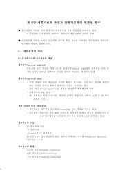
Example: Viterbi algorithmThis handout illustrates a specific example of the Viterbi algorithm with the purpose of unifyingthe concepts introduced in the application report, “Viterbi Decoding Techniques in theTMS320C54x Family”.The convolution coder is often used in digital transmission systems where the signal to noise ratiois very low rendering the received signal error prone. The convolution coder achieves error freetransmission by adding enough redundancy to the source symbols. The choice of the convolutionalcode is application dependent and varies with the frequency characteristics of the transmissionmedium as well as the desired transmission rate.The Viterbi algorithm is a method commonly used for decoding bit streams encoded by convolutioncoders. The details of a particular decoder algorithm depends on the encoder. The Viterbialgorithm is not a single algorithm that can be used to decode coded bit streams of any convolutioncoder.The system chosen to illustrate the encoding and Viterbi decoding process is a 4-state optimal rate1/2 convolutional code. A block diagram of this convolution encoder is show in Figure 1. xn ( ) isthe input and G 0( n) and G 1( n)are the encoded outputs. The rate of the convolution coder isdefined as the number of input bits to output bits. This system has 1 input and 2 outputs therebyresulting in a coding rate of 1/2. The number of states of a convolution coder is determined by itsnumber of delay units. There are 2 delay units in this system and therefore, there are 2 2 = 4states. For a system with k delay units, there are 2 k states.++G (n)0x(n)Dx(n-1)Dx(n-2)+G (n)1FIGURE 1. Block diagram of convolutional encoderThe system block diagram can be expressed with the following equations.G 0 ( n) = xn ( ) + xn ( – 1) + xn ( – 2)G 1 ( n) = xn ( ) + xn ( – 2)The state diagram of this system is depicted in Figure 2. The states are defined as x(n-1),x(n-2)pairs and the state transitions are defined as G 0 ( n) , G 1 ( n)/ xn ( ). The states are indicative of systemmemory. The state transitions gives you the path and the outputs associated with a giveninput. Since a state transition is associated with each possible input, the number of state transitionsdepends on the number of possible inputs. If there are m inputs, then there will be 2 m statetransitions. The total number of state transitions at a point in time is the product of the number of

state transitions and the number of states, .2 m k00/00011/011/1+ 110100/110/01001/001/1x(n-1),x(n-2)10/1G (n),G (n)/x(n)0 1FIGURE 2. State diagram.The state diagram offers a complete description of the system. However, it shows only the instantaneoustransitions. It does not illustrate how the states change in time. To include time in statetransitions, a trellis diagram is used (Figure 3). Each node in the trellis diagram denotes a state ata point in time. The branches connecting the nodes denote the state transitions. Notice that theinputs are not labeled on the state transitions. They are implied since the input, xn ( ), is includedin the destination states, xn ( ),xn ( – 1). Another thing to note is that the state transitions are fixedby the definition of the source, xn ( – 1) , xn ( – 2), and the destination states. The state transitionsare independent of the system equations. This a consequence of including the input, xn ( ), in thestate definition. In certain systems, definition of the states may be more complicated and mayrequire special considerations. Explanation of such systems (such as the radix 4 trellis) is outsidethe scope of this example.Origional TrellisReordered Trellisx(n-1),x(n-2)G0,G1x(n),x(n-1)x(n-1),x(n-2)G0,G1x(n),x(n-1)000110110010000000000011 1111110101 0010011010100101 010110 11111011FIGURE 3. Trellis diagramsThere are two trellis diagrams shown in Figure 3. They differ only in the way the destinationstates are ordered. The purpose for reordering is to obtain higher computational efficiency. Thereordered trellis is partitioned into groups of states and state transitions that are isolated fromother such groups. This allows realizable, specialized hardware to be designed that is dedicated tocompute parameters associated with the particular group. The structure of the groups shown in

Figure 3 is called the “butterfly” due to the physical resemblance. It is also referred to as the radix-2 trellis structure since each group contains 2 source and 2 destination states. The TMS320C54xDSP’s has specialized hardware that is dedicated to compute parameters associated with a butterfly.Note, again, that the structure of the reordered trellis is fixed depending on how the states aredefined. Not all trellis diagrams can be reordered into butterflies. Fortunately, a number of commonlyused convolution coders have this nice property.An important feature of this convolution code is that in each butterfly, there are only two (out offour possible) distinct outputs: 00 and 11; or 01 and 10. Notice that the hamming distance of eachoutput pairs is 2. This feature is available to a very small subset of all possible convolution codes.The usefulness of the this feature will be apparent later on when Viterbi decoding is described.Figure 4 illustrates the entire process of encoding an input pattern to quantizing the received signalto decoding the quantized signal. The sample input pattern used is 1011010100. For the purposeof this example, this input pattern is sufficiently long. In practice, for proper error correction,the input pattern need to be longer than approximately 10 times the number of delay units plus 1,i.e. length of input pattern = 10( k + 1). ( k + 1)is often referred to as the constraint length. Forthis example, k=2 which implies 30 input symbols need to be received before decoding toimprove the bit error rate.The first trellis diagram in Figure 4 illustrates the state transitions associated with each input. Thistrellis diagram is used here to illustrate how the decoder operates. Use Figure 3 to verify the statetransitions and the encoder outputs. The encoder outputs do not have to be generated using thetrellis diagram. They can be generated using the system equations directly.The encoded outputs are transmitted as signed antipodal analog signals (i.e. 0 is transmitted witha positive voltage and 1 is transmitted with a negative voltage). They are received at the decoderand quantized with a 3-bit quantizer. The quantized number is represented in 2’s complement givingit a range of -4 to 3. The process of quantizing a binary analog signal with a multi-bit quantizeris called soft decision. In contrast, hard decision quantizes the binary analog signal using a 1-bit quantizer (i.e. quantized signal is either 0 or 1). Soft decision offers better performance resultssince it provides a better estimate of the noise (i.e. less quantization noise is introduced). In mostcircumstances, the noise is strong enough just to tip the signal over the decision boundary. If harddecision is used, a significant amount of quantization noise will be introduced. The quantized softdecision values are used to calculate the parameters for the Viterbi decoder.Up to this point, no Viterbi decoding has been performed. Viterbi decoding begins after a certainnumber of encoded symbols have been received. This length, again, is usually longer than10( k + 1)and is application dependent. In this example, 20 encoded symbols are received beforebeing decoded. In some applications, Viterbi decoding is operated on a frame of received symbolsand is independent of the neighboring frames. Is is also possible to perform Viterbi decoding on asliding window in which a block of decoded bits at the beginning of the window is error free, andthe windows will have to overlap. With frame by frame decoding, a number of trailing zerosequalling to the number of states is added. This forces the last state of the frame to be zero providinga starting point for traceback. With sliding window decoding, the starting point for tracebackis the state with the optimal accumulated metric. This starting state may be erroneous. However,the traceback path will converge to the correct states before reaching the block of error free bits.

INTRODUCTIONOn December 16, 2003, an amended complaint was filed by nine North Dakotaschool districts requesting that the state’s public school finance system be declaredunconstitutional. The state has denied and continues to deny the core complaint broughtforward by the plaintiffs.On January 10, 2006, the parties in opposition determined that it was desirable forthem to stay the action and provide the North Dakota Legislative Assembly with theopportunity to settle, compromise, and resolve this action on certain terms and conditions.Consequently, the parties executed an “Agreement to Stay Litigation.” The document isattached as Exhibit A.The first condition accepted by both parties was that the Governor issue anExecutive Order creating a North Dakota Commission on Education Improvement. Thedocument, as currently amended, is attached as Exhibit B. The Commission membersinclude the Superintendent of Public Instruction, four school district administrators, andfour legislators. The Commission also includes four non-voting members. Three representthe state’s teachers, school boards, and school administrators, and the remaining individualserves as a special advisor on the school funding formula.The Commission was instructed to prepare a report recommending ways to improvethe current system of delivering and financing elementary and secondary education,1.

where n denotes the time instance and i denotes the path calculated for. The above equation can befurther simplified by observing the expansion:∑∑Going back to Figure 4, the branch metrics can now be calculated using the above local distanceequation. As an example, the branch metrics for time 0 and 1 is calculated here. The receivedquantized soft decision pair is (-3,-4). The branch metric corresponding to( G 0( n) , G 1( n)) = ( 00 , ) is equal to – 3( 1)– 4( 1)= – 7. For ( G 0( n) , G 1( n)) = ( 01 , ), it is– 31 ( ) – 4( – 1)= 1. For ( G 0( n) , G 1( n)) = ( 10 , ), it is – 3( – 1)– 4( 1)= – 1. And for( G 0 ( n) , G 1 ( n)) = ( 11 , ), it is – 3( – 1)– 4( – 1)= 7. Notice that the G j ( n)‘s used in the localdistance calculation are +1 and -1, rather than +3 and -4 respectively. There are three reasons.First, using unities makes computation very simple. The branch metrics can be calculated by addlocaldistance( ni , ) = [ S 2 j( n) – 2S j( n)G j( n) + G 2 j( n)]all jand noting that S 2 j( n)and G 2 j( n)are constants in a given symbol period. These terms canall j∑all jbe ignored since we are concerned with finding the minimum local distance path. The followingmeasure will suffice for determining the local distance: Note that the -2 is taken out which implieslocal distance 1 ( ni , ) = S j ( n)G j ( n)that instead of finding the path with the minimum local distance, we would look for the path withthe maximum local distance 1( ni , ).∑all jOriginating states: 00, 01Originating states: 10, 11G (n)1(3,3)(-4,3)G (n)1G (n)0G (n)0(-4,-4)(3,-4)Decision boundariesFIGURE 6. Signal constellation for Viterbi decoding

ing and subtracting the soft decision values. Second, 3 and -4 can be scaled to approximately 1and -1 respectively. As mentioned in the derivation of local distance 1 , constant scaling can beignored in determining the maxima and the minima. Finally, note that there are only two uniquemetric magnitudes, 1 and 7. Therefore, to compute the branch metric, you only need to do 1 add,1 subtract, and 2 negation.Once the branch metrics are calculated, the state metrics and the best incoming paths for each destinationstates can be determined. The state metrics at time 0 are initialized to 0 except for state00, which takes on the value of 100. This value is arbitrarily chosen and is large enough so that theother initial states cannot contribute to the best path. This basically forces the traceback to convergeon state 00 at time 0.The state metrics are updated in two steps. First, for each of the two incoming paths, the correspondingbranch metric is added to the state metric of the originating state. The two sums arecompared and the larger one is stored as the new state metric and the corresponding path is storedas the best path. Take state 10 at time instance 2 for example (Figure 4). The two paths coming into this state originates from states 00 and 01 (Figure 3). Looking at the second trellis, we see thatstate 00 has a value of 93 and state 01 has a value of 1. The branch metric of the top path (connectingstate 00 at time 1 and state 10 at time 2) is 1. The branch metric of the bottom path (betweenstates 01 and 10) is -1. The top path gives a sum of 93 + 1 = 94 and the bottom path give a sumof 1+ (–1)= 0. As a result, 94 is stored as the state metric for state 10 at time 2 and the top pathis stored as the best path in the transition buffer.The transition buffer stores the best incoming path for each state. For a radix 2 trellis, only 1 bit isneeded to indicate the chosen path. A value of 0 indicates that the top incoming path of the givenstate is chosen as the best path whereas a value of 1 indicates that the bottom path is chosen. Thetransition bits for our example is illustrated in Figure 4 in the third trellis.Traceback begins after completing the metric update of the last symbol in the frame. For frame byframe Viterbi decoding, all that is needed by the traceback algorithm are the state transitions. Thestarting state is state 00. For sliding window decoding, the starting state is the state with the largeststate metric. In our example, the starting state for both types of decoding is 00 since it has thelargest state metric, 158. Looking at the state transition for state 00, we see that the bottom path isoptimal (state transition = 1 implies bottom path). Two things now happen. First, the transition bit,1, is sent to the decoder output. Second, the originating state, state 01, of this optimal path isdetermined. This process is repeated until time 2, which corresponds to the first input bit transmitted.The decoded output is shown in Figure 4 in the last row. Notice that the order with which thedecoded output is generated is reversed, i.e. decoded output = 10101101 whereas the sample inputpattern is 10110101. Additional code need to be added to reverse the ordering of the decoded outputto exactly reconstruct the sample input.