Lattice sums arising from the Poisson equation - David H Bailey

Lattice sums arising from the Poisson equationD H Bailey 1 , J M Borwein 2 , R E Crandall 3 (1947-2012), I J Zucker 41 Lawrence Berkeley National Lab, Berkeley, CA 94720; University of California, Davis,Department of Computer Science, Davis, CA 95616E-mail: david@davidhbailey.comSupported in part by the Director, Office of Computational and Technology Research,Division of Mathematical, Information, and Computational Sciences of the U.S. Departmentof Energy, under contract number DE-AC02-05CH11231.2 Centre for Computer Assisted Research Mathematics and its Applications (CARMA),University of Newcastle, Callaghan, NSW 2308, Australia,E-mail: jonathan.borwein@newcastle.edu.au3 Center for Advanced Computation, Reed College, Portland OR4 Department of Physics, Kings College London,E-mail: jzucker@btinternet.com

Lattice sums arising from the Poisson equation 2Abstract: In recent times, attention has been directed to the problem of solving the Poissonequation, either in engineering scenarios (computational) or in regard to crystal structure(theoretical). Herein we study a class of lattice sums that amount to Poisson solutions, namelythe n-dimensional formsφ n (r 1 , . . . , r n ) = 1 π 2 ∑m 1 ,...,m n odde iπ(m 1r 1 +···+m nr n).m 2 1 + · · · + m 2 nBy virtue of striking connections with Jacobi ϑ-function values, we are able to develop newclosed forms for certain values of the coordinates r k , and extend such analysis to similarlattice sums. A primary result is that for rational x, y, the natural potential φ 2 (x, y) is 1 π log Awhere A is an algebraic number. Various extensions and explicit evaluations are given. Suchwork is made possible by number-theoretical analysis, symbolic computation and experimentalmathematics, including extensive numerical computations using up to 20,000-digit arithmetic.

Lattice sums arising from the Poisson equation 31. About this paperIn this paper, we analyze various generalized lattice sums [7], which have been studied formany years in the mathematical physics community, for example in [7, 13, 14] and a recentfascinating work on cyclotomic polylogarithms and corresponding multiple harmonic sums [1].Recently our own interest has been triggered by some intriguing research in practical imageprocessing techniques [9]. These developments have underscored the need to better understandthe underlying theory behind both lattice sums and the associated Poisson potential functions.To that end, we present a number of results, perhaps the most notable of which is theremarkable fact that, for rational x and y, the most natural two-dimensional Poisson potentialfunction satisfiesφ 2 (x, y) = 1 ∑ cos(mπx) cos(nπy)= 1 log A, (1)π 2m 2 + n 2 πm,n oddwhere A is an algebraic number, or, in other words, the root of an integer polynomial, whosedegree and coefficients depend on x and y.In Section 2, we describe, consistent with [9], the underlying equations along with “natural”Madelung constants and relate them to the classical Madelung constants. In Section 3, weproduce the solution φ n which, especially with n = 2, provide the central objects of our study.In Section 4, we develop rapid methods of evaluating φ n .These fast methods are used in Section 5 to experimentally determine closed-formevaluations for φ 2 (x, y) for some specific x and y, such asπ 2 φ 2 (1/5, 2/5) =∑m,n oddcos(mπ/5) cos(2nπ/5)m 2 + n 2 ? = π 16log 5. (2)We are also able to prove a few of the simpler evaluations (see Theorem 3 and AppendicesI and III). From this and further computational evidence, we conjectured the algebraic resultmentioned above in (1), which is stated and proven as Theorem 10 of Section 6. This resultwas made possible because earlier in Section 6 we relate φ 2 , and its counterpart sum over evenintegers ψ 2 , in terms of general Jacobean theta functions ϑ k (z, q) for k = 1, ..., 4. In Section6.4, we also touch on generalizations to sums of the formφ 2 (x, y, d) := 1 ∑ cos(πmx) cos(πn √ d y), (3)π 2 m 2 + dn 2m,n oddfor rational d > 0.In Section 7, we describe the quite extensive and challenging computational experimentswe have undertaken, and summarize the results in tabular form. In Section 8, we briefly lookat the state of our knowledge in three and four dimensions. Finally, in three Appendices, wepresent some additional details of our proofs via factorization of lattice sums.

Lattice sums arising from the Poisson equation 42. Madelung entitiesIn a recent treatment of ‘natural’ Madelung constants [9] it is pointed out that the Poissonequation for an n-dimensional point-charge source,∇ 2 Φ n (r) = − δ(r), (4)gives rise to an electrostatic potential—we call it the bare-charge potential—of the formΦ n (r) =Γ(n/2 − 1)4π n/2 1r n−2 =:C n, if n ≠ 2, (5)rn−2 Φ 2 (r) = − 12π log r =: C 2 log r, (6)where r := |r|. Since this Poisson solution generally behaves as r 2−n , the previous work [9]defines a “natural” Madelung constant N n as (here, m := |m|):′∑ (−1) 1·mN n := C n , if n ≠ 2, (7)mn−2 m ∈ Z n′∑N 2 := C 2m ∈ Z n (−1) 1·m log m,where in cases such as this log sum one must infer an analytic continuation [9], as the literalsum is quite non convergent. This N n coincides with the classical Madelung constantM n :=′∑(−1) 1·mmm ∈ Z nonly for n = 3 dimensions, in which case N 3 = 14π M 3. But in all other dimensions there is noobvious M, N relation.A method for gleaning information about N n is to contemplate the Poisson equation witha crystal charge source, modeled after NaCl (salt) in the sense of alternating lattice charges:∇ 2 φ n (r) = − ∑m ∈ Z n (−1) 1·m δ(m − r). (9)Accordingly—based on the Poisson equation (4)—solutions φ n can be written in terms of therespective bare-charge functions Φ n , asφ n (r) =∑(−1) 1·m Φ n (r − m). (10)m ∈ Z n2.1. Madelung variantsWe have defined the classical Madelung constants (8) and the “natural Madelung constants(7). Following [9], we define a Madelung potential, now depending on a complex s and spatial(8)

Lattice sums arising from the Poisson equation 5point r ∈ Z n :M n (s, r) := ∑ (−1) 1·p|p − r| , (11)s p ∈ Z nWe can write limit formulae for our Madelung variants, first the classical Madelung constantM n := lim(M n (1, r) − 1 )(12)r → 0 r=′∑(−1) 1·ppp ∈ Z nand then the “natural” Madelung constant, (13)N n := lim (φ(r) − Φ(r))r → 0(14)′∑ (−1) 1·p= C n .p n−2 p ∈ Z n (15)For small even n this last sum is evaluable. For example, from [6, Eqn. (9.2.5)] we have′∑which with s = 1 yieldsp∈Z 4 (−1) 1·pp 2s = (1 − 2 2−s )(1 − 2 1−s )ζ(s)ζ(s − 1), (16)N 4 = − 1 log 2.π2 Similarly [6, Exercise 4b), p. 292] derives′∑p∈Z 8 (−1) 1·pp 2s = − 16(1 − 2 4−s )ζ(s)ζ(s − 3), (17)which with s = 3 determines thatN 8 = − 4 π 4 ζ(3).Generally, via the Mellin transform M s ϑ 2n4 (q), see below, for small n values of N 2n aresimilarly susceptible. For instance with G denoting Catalan’s constantN 6 = − 124π − 2Gπ , 3given in [9]. The more complex value N 2 is presented in (26).

Lattice sums arising from the Poisson equation 62.2. Relation between crystal solutions φ n and Madelung potentialsFrom (5), (10), and (11) we have the general relation for dimension n ≠ 2,φ n (r) = C n M n (n − 2, r). (18)Note that for the case n = 3, the solution φ 3 coincides with the classical Madelung potentialM 3 (1, r) in the senseφ 3 (r) = 14π M 3(1, r),because C 3 = 1/(4π). Likewise, the “natural” and classical Madelung constants are related4π N 3 = M 3 . The whole idea of introducing ‘natural’ Madelung constants N n is that thiscoincidence of radial powers for φ and M potentials holds only in 3 dimensions. For example,in n = 5 dimensions, the summands for φ 5 and M 5 (1, ·) involve radial powers 1/r 3 , as inφ 5 (r) = 18π 2 M 5(3, r).3. The crystal solutions φ nIn [9] it is argued that a solution to (9) isφ n (r) = 1 ∑∏ nk=1 cos(πm kr k ), (19)π 2m 2 m ∈ O nwhere O denotes the odd integers (including negative odds). These φ n do give the potentialwithin the appropriate n-dimensional crystal, in that φ n vanishes on the surface of the cube[−1/2, 1/2] n , as is required via symmetry within an NaCl-type crystal of any dimensions. Torender this representation more explicit and efficient, we could write equivalentlyφ n (r) = 2nπ 2∑m 1 ,...,m n > 0, oddcos(πm 1 r 1 ) · · · cos(πm n r n ).m 2 1 + · · · m 2 nIt is also useful that—due to the symmetry inherent in having odd summation indices—we cancavalierly replace the cosine product in (19) with a simple exponential:φ n (r) = 1 ∑ e iπm·rπ 2 m . (20)2 m ∈ O nThis follows from the simple observation that ∏ exp(πim k r k ) = ∏ (cos(πm k r k ) + i sin(πm k r k )),so when the latter product is expanded out, the appearance of even a single sin term isannihilating, due to the bipolarity of every index m k .

Lattice sums arising from the Poisson equation 7We observe that convergence of these conditionally convergent sums is by no means obviousbut that results such as [7, Thm. 8.3 & Thm. 8.5] ensure thatφ n (r, s) := 1 ∑∏ nk=1 cos(πm kr k ), (21)π 2m 2s m ∈ O nis convergent and analytic with abscissa σ 0 for (n − 1)/4 ≤ σ 0 ≤ (n − 1)/2 where Re(s) = σ.For the central case herein, summing over increasing spheres is analytic in two dimensionsfor σ 0 ≤ 23/73 < 1/2 and in three dimensions for σ 0 ≤ 25/34 < 1, but in general the bestestimate we have is σ 0 ≤ n/2 − 1, so for n ≥ 5 to avoid ambiguity we work with the analyticcontinuation of (21) from the region of absolute convergence with σ > n/2. Indeed, all ourtransform methods are effectively doing just that.4. Fast series for φ nFrom previous work [9] we know a computational seriesφ n (r) = 12π∑ sinh(πR(1/2 − |r 1 |) ∏ n−1k=1 cos(πR kr k+1 ), (22)R cosh(πR/2)R ∈ O n−1suitable for any nonzero vector r ∈ [−1/2, 1/2] n . The previous work also gives an improvementin the case of n = 2 dimensions, namely the following form for which the logarithmic singularityat the origin has been siphoned off:φ 2 (x, y) = 1 cosh(πx) + cos(πy)log4π cosh(πx) − cos(πy) − 2 π∑ cosh(πmx) cos(πmy)m(1 + e πm )m ∈ O +. (23)These series, (22) and (23) are valid, respectively, for r 1 , x ∈ [−1, 1].For clarification, we give here the (n = 3)-dimensional case of the fast series:( √ )φ 3 (x, y, z) = 2 π∑ sinh p2 + q2 2 (1 − 2|x|) cos(πpy) cos(πqz)√ ( √ ) . (24)πp2 + q 2 cosh p2 + q 2p,q > 0, oddThough it may not be manifest in this asymmetrical-looking series, it turns out that for anydimension n the φ n (r 1 , · · · r n ) is invariant under permutations and sign-flips. For example,φ 3 (x, y, z) = φ 3 (−y, z, −x) and so on. It thus behooves the implementor to consider x—whichappears only in the first sum of (24)—to be the largest in magnitude of the three coordinates, foroptimal convergence. A good numerical test case which we mention later is the exact evaluationφ 3 (1/6, 1/6, 1/6) = √ 3, which we have confirmed to 500 digits.4ππ2

Lattice sums arising from the Poisson equation 8With n > 2 it is not clear how best to isolate the (r = 0) singularity in higher dimensions.One approach—possibly not optimal, is to derive [9]′∑ (−1) 1·mN n = C nm n−2m ∈ Z +(n−1)− 1 ∑π1,R(1 + e πR )if n ≠ 2 (25)R ∈ O n−1∑′then employ a fast series for the C n term [9]. In fact, it is often possible to give this m-sumhere a closed form [9], so that a great many N n are now resolved. (More generally speaking,we cannot yet resolve any of the N odd n>1 .)4.1. Closed form for the “natural’ Madelung constant N 2The (n = 2)-dimensional natural Madelung constant has also been resolved on the basis of (23)(see [9]), to take the valueN 2 = 14π log 4 Γ4 (3/4). (26)π 3We remind ourselves that this closed form was achieved by contemplating the limiting processr → 0, and hence Coulomb-singularity removal.We also record the following numerically effective Mellin transform for n > 2N n = − 1 ∫ ∞( ( ))1 − ϑn4π4 e−πxx n/2−2 dx < 0, (27)0where the integral is positive since 0 < ϑ 4 (q) < 1 for 0 ≤ q ≤ 1.From this the large n behavior of N n may be estimated as( )Γ(n/2 − 1) n n(n − 1)N n ≍ − · − + ... , (28)π n/2 2 2 n/2on approximating ϑ 4 (q) = 1 − 2q + O (q 4 ) and 1 − x n = −n(x − 1) + n(n − 1)/2 (x − 1) 2 +O ( (x − 1) 3) and then integrating term-by-term. For instance, from (27) we computeN 100 = −8.6175767047403040779... × 10 37while the asymptotic (28) givesN 100 ≍ −8.6175767047403038... × 10 37 .Indeed, we can make effective estimates, as in:Theorem 1 (Effective bounds on N n ). For integer n > 2 we have−1 +n2 n/2−1 > N n(Γ(n/2−1)π n/2) > −1. (29)n2

Lattice sums arising from the Poisson equation 9Proof. Let q := exp(−πt) and note1 − 2q ≤ ϑ 4 (q) ≤ 1 − 2q + 2q 4 .Now for any x ∈ (0, 1) and positive integer n it is elementary that1 − nx ≤ (1 − x) n ≤ 1 − nx + n(n − 1)x 2 /2.Putting x := ϑ 4 (q) here, knowing x ∈ [1 − 2q, 1 − 2q + 2q 4 ] in the integral representation (27)quickly gives both bounds of the theorem.Remark 2. Another approach to these effective error bounds is to noteN n= C n∑N≥1r n (N)(−1) NN n/2−1 ,where r n (N) counts the number of n-square representations of N. Indeed, the first asymptoticterms in (28) arise immediately from the observationr n (1) = 2n,as every representation of 1 is (±1) 2 + 0 2 + . . . + 0 2 , and similarlyr n (2) = 1 n(n − 1) · 4.2In this regard, the rapid decrease in asymptotic terms for large n makes intuitive sense. Indeed,in high dimensions, a “great deal” of the natural potential is due to charges that reside “nearthe origin.”Also, applying the theta transform [6, Eqn. (2.3.2)] in (27) yields the analytically usefulN n = − 14π{ ∫ 2 1n − 2 −0ϑ n 4( ) ∫ 1( (e−π tt n/2−2 dt + t −n/2 − ϑ )) }n2 e−π tdt , (30)where numerical care is needed near the origin in the second integrand.In the next section we derive certain closed forms and exhibit others determinedexperimentally—most of which we also indicate how to prove.0✸5. Closed forms for the φ 2 potentialProvably we have the following results which were established by factorization of lattice sumsafter being empirically discovered by the methods described in the next few sections.

Lattice sums arising from the Poisson equation 10Theorem 3. We haveProof. Consider for s > 0φ 2 (1/3, 1/3) = 18π log(1 + 2/√ 3), (31)φ 2 (1/4, 1/4) = 14π log(1 + √ 2), (32)φ 2 (1/3, 0) = 18π log(3 + 2√ 3). (33)V 2 (x, y; s) :=∞∑m,n=−∞cos[π(2m + 1)x] cos[π(2n + 1)y][(2m + 1) 2 + (2n + 1) 2 ] s . (34)This V 2 function will be related by normalization, as V 2 (x, y; 1) = π 2 φ 2 (x, y). Treating it assome general lattice sum [6, 7], we derive (with some difficulty; more details are in Appendix I)V 2 (1/3, 1/3; s) = 2 −1−s [ −(1 − 2 −s )(1 − 3 2−2s )L 1 (s)L −4 (s)+3(1 + 2 −s )L −3 (s)L 12 (s) ] . (35)The L’s in (35) are various Dirichlet series, L 1 being the Riemann ζ function. Note that(1 − 3 2−2s ) factors as (1 + 3 1−s )(1 − 3 1−s ) and lim s→1 (1 − 3 1−s )L 1 (s) = log 3, and thatL −4 (1) = π √3π4 , L −3(1) =9 , L 12(1) = √ 1 log(2 + √ 3). (36)3After gathering everything together we have(φ 2 (1/3, 1/3) = 1 π V 2(1/3, 1/3, 1) = 12 8π log 3 + 2 √ )3,3which is (31).More simplyV 2 (1/4, 1/4; s) = 2∞∑m,n=−∞is a familiar lattice sum [6, 7]. So withwe deriveL −8 (1) =π2 √ 2φ 2 (1/4, 1/4) = 14π log(1 + √ 2).which is (32).(−1) m+n[(4m − 1) 2 + (4n − 1) 2 ] s = 21−s L −8 (s)L 8 (s) (37)and L 8 (1) = 1 √2log(1 + √ 2) (38)

Lattice sums arising from the Poisson equation 11Likewisewhich yieldsV 2 (1/3, 0; s) = 2 −1−s [ (1 − 2 −s )(1 − 3 2−2s )L 1 (s)L −4 (s)+3(1 + 2 −s )L −3 (s)L 12 (s) ] (39)φ 2 (0, 1/3) = 116π log (3(2 + √ 3) 2 )= π 8 log(3 + 2√ 3),which is (33).Using the integer relation method PSLQ [5] to hunt for results of the form,exp (πφ 2 (x, y))?= α, (40)for α algebraic we may obtain and further simplify many results such as:Conjecture 4. We have discovered and subsequently provenφ 2 (1/4, 0)φ 2 (1/5, 1/5)φ 2 (1/6, 1/6)φ 2 (1/3, 1/6)φ 2 (1/8, 1/8)φ 2 (1/10, 1/10)?= 14π log α where α + 1/α2?=(18π log 3 + 2 √ 5 + 2?= 14π log γ where γ + 1/γ2?= 14π log τ where τ − 1/τ2(?= 14π log 1 + √ 2 − √ )24√2 − 1?= 14π log µ where µ + 1/µ2= √ 2 + 1√5 + 2 √ )5 ,= √ 3 + 1= (2 √ 3 − 3) 1/4= 2 + √ 5 +√5 + 2 √ 5?where the notation = indicates that we originally only had experimental (extreme-precisionnumerical) evidence of an equality.Looking at (14) and (26), we can take the most valuable (in the sense of (x, y) being closestto the origin (0, 0)) of the above φ 2 evaluations, and attempt an approximationN 2 ≈ φ 2 (1/10, 1/10) + 12π log √ 1/100 + 1/100 = −0.09818 . . . ,which is off of the correct analytic N 2 value −0.0982599931 . . . by about 1 part in 1000.

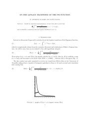
Lattice sums arising from the Poisson equation 12Figure 1. High-precision plot of the Monge surface z = φ 2 (x, y), via fast series (23), showingthe logarithmic origin singularity (plot adapted from [9]). In this plot, x, y range over the 2-cube[−1/2, 1/2] 2 ; from symmetry one only need know the φ 2 surface over an octant 1/2 > x ≥ y > 0,say. We are able to establish closed forms for heights on this surface above certain rationalpairs (x, y). As just one example, φ 2 (1/4, 1/4) = 14π log(1 + √ 2) ≈ 0.0701.Such hunts are made entirely practicable by (23). Note that for general x and y we haveφ 2 (y, x) = φ 2 (x, y) = −φ 2 (x, 1−y), so we can restrict searches to 1/2 > x ≥ y > 0, as illustratedin Figure 1.The following hints at how much underlying algebraic structure there is:Example 5 (Denominator of five). We record thatφ 2 (1/5, 1/5)?= log(α)/π and φ 2 (2/5, 2/5)?= log(β)/πwhere α > β are the positive roots of x 32 − 12 x 24 − 26 x 16 + 52 x 8 + 1. Similarly,φ 2 (1/5, 0/5)?= log(α)/π and φ 2 (2/5, 0/5)?= log(β)/πshare the positive roots of x 32 − 52 x 24 − 26 x 16 + 12 x 8 + 1. Moreover,?φ 2 (1/5, 2/5) = 1 log 5, (41)16πwhich is stunningly simple. Explicitly,∑ cos(mπ/5) cos(2nπ/5)= ? π log 5n 2 + m 2 64 . (42)0

Lattice sums arising from the Poisson equation 13Example 6 (Denominator of six and more). Likewise,φ 2 (1/6, 0)for α the largest root ofSimilarly,?= log(α)/πx 16 − 4 x 14 + 4 x 12 − 4 x 10 − 2 x 8 − 4 x 6 + 4 x 4 − 4 x 2 + 1.φ 2 (1/8, 0)?= log(β)/π and φ 2 (1/10, 0)?= log(γ)/πfor β, γ the largest roots respectively of(√ )(√ )(√ )x 32 + 8 2 + 1 x 28 − 12 x 24 − 8 2 + 1 x 20 − 38 x 16 − 8 2 + 1 x 12(√ )− 12 x 8 + 8 2 + 1 x 4 − 1(the integer polynomial is of degree 64) and(√ ) (x 8 − 5 + 1 x 6 − 5 3/4 + 3 5 1/4 + √ )5 + 1 x 4 −(√5 + 1)x 2 + 1(the integer polynomial is now degree 32). In each case the polynomial is palindromic. Again,the polynomial found for x 1/4 is simpler. For 1/6 it is x 8 − 8x 7 − 20x 6 − 56x 5 − 26x 4 − 56x 3 −20x 2 − 8x + 1.Likewise,φ 2 (1/3, 1/4)for σ the largest root of?= log(σ)/4πx 8 + 4 x 7 − 4 x 6√ 3 − 4 x 5 +(14 − 8 √ )3 x 4 − 4 x 3 − 4 x 2√ 3 + 4 x + 1.We have also discovered that for k = 1, 2, 3 we have?φ 2 (k/7, k/7) = 18π log(α k)where α 1 > α 2 > α 3 are the positive roots of(7 x 6 − 154 + 56 √ ) (7 x 5 − 1603 + 616 √ ) (7 x 4 + 9156 + 3472 √ )7(− 4431 + 1680 √ ) (7 x 2 − 4298 + 1624 √ )7 x − 8 √ 7 − 21.x 3Also,φ 2 (2/7, 1/7)and φ 2 (3/7, 1/7)?= 116π log(β 1), φ 2 (3/7, 2/7)?= 116π log(β 3),?= 116π log(β 2),

Lattice sums arising from the Poisson equation 14where β 1 > β 2 > β 3 are the positive roots ofx 6 − 14 x 5 − 3801 x 4 + 9436 x 3 − 1281 x 2 − 238 x − 7,all of whose roots are real. Finallyφ 2 (1/7, 0)and φ 2 (5/7, 0)?= 18π log(γ 1), φ 2 (3/7, 0)?= 18π log(γ 3),where γ 1 > γ 2 > γ 3 are the positive roots of(x 6 − 98 + 40 √ ) (7 x 5 + 24 √ )7 + 147 x 4 +(+ 14 − 8 √ )7 x − 8 √ 7 + 21.?= 18π log(γ 2)(308 + 48 √ ) (7 x 3 − 16 √ )7 − 119 x 2Similar observations appeared to work for denominators of 3 ≤ n ≤ 15. For instance, thequantity exp (4π φ 2 (1/13, 3/13)) was found to be of degree 36 over Q (√ 3 ) .✸Remark 7 (Algebraicity). In light of our current evidence we conjecture that for x, y rational,?φ 2 (x, y) = log απfor α algebraic. Theorem 10 will prove this conjecture.Remark 8. The proven results of Theorem 3 rely on the special structure of the series (35),(37) and (39). But conjecturally, as we have seen and will see below, much more is true anddoes not apparently rely on the complete factorizations [20] of (34) used above.We might try to work backwards and find the expressions they came from for generals. However, φ 2 (1/4, 0; s) in particular cannot be expressed in terms of Dirichlet series withreal characters. This then is a candidate for the use of complex character Dirichlet series [7].Moreover, (41) suggests another approach might be more fruitful. This is indeed so as Theorem9 and its sequela show. ✸We note that Theorem 10 proves that all values should be algebraic but does not, a priori,establish the precise values we have found. This will be addressed in §6.2.(43)✸6. Madelung and “jellium” crystals and Jacobi ϑ-functionsWe have studiedφ 2 (x, y) := 1 π 2∑a,b ∈ Ocos(πax) cos(πby)a 2 + b 2 , (44)

Lattice sums arising from the Poisson equation 15as a ‘natural” potential for n = 2 dimensions in the Madelung problem. Here E denotes theeven integers. There is another interesting series, namelyψ 2 (x, y) := 1′∑4π 2a,b ∈ Z= 1 π 2 ∑a,b ∈ Ecos(2πax) cos(2πby)a 2 + b 2cos(πax) cos(πby)a 2 + b 2 , (45)where E denotes the even integers.Now it is explained, and pictorialized in [9] that this ψ 2 function is the ‘natural” potentialfor a classical jellium crystal and relates to Wigner sums [7]. This involves a positive charge atevery integer lattice point, in a bath—a jelly–of uniform negative charge density. As such, theψ functions satisfy a Poisson equation but with different source term [9].Note importantly that ψ 2 satisfies Neumann boundary conditions on the faces of the Delordcube—in contrast with the Dirichlet conditions in the Madelung case.Briefly, a fast series for ψ n has been worked out [9] as:ψ n (r) = 1 12 + 1 2 r2 1 − 1 2 |r 1| + 2n−3πvalid on the Delord n-cube, i.e. for r ∈ [−1/2, 1/2] n .∑ cosh(πS(1 − 2|r 1 |) ∏ n−1k=1 cos(2πS kr k+1 ),S sinh(πS)S∈Z +(n−1)(46)6.1. Closed forms for ψ 2 and φ 2Using the series (46) for high-precision numerics, it was discovered (see [9, Appendix]) thatprevious lattice-sum literature has harbored a longtime typographical issue for certain 2-dimensional sums, and that a valid closed form for ψ 2 is actuallyψ 2 (x, y) = x22 + 1 () Γ(1/4)4π log √ − 18π Γ(3/4) 2π log ∣ ( )∣ ϑ1 π(ix + y), e−π ∣ . (47)As for the Madelung scenario, it then became possible to cast φ 2 likewise in closed form,namelyφ 2 (x, y) = 14π log |α(z)| where α(z) := ϑ2 2(z, q)ϑ 2 4(z, q)ϑ 2 1(z, q)ϑ 2 3(z, q)for q := e −π , z := π 2(y + ix). (See [9] and Appendix II for details.)Now we observe that, using classical results [6, §2.6 Exercises 2 and 4] on theta functions(also described in [16]), we may also write(48)

Lattice sums arising from the Poisson equation 16Theorem 9. For z := π (y + ix)2φ 2 (x, y) = 1 ∣ ∣ ∣∣∣∣2π log ϑ 2 (z, q)ϑ 4 (z, q)ϑ 1 (z, q)ϑ 3 (z, q) ∣ = 1 ∣∣∣∣4π log 1 − λ(z) √ ∣∣∣∣2, (49)1 − 1/λ(z) √2andwhereandwith q := e −π .ψ 2 (x, y) = − 14π log ∣ ∣∣2 µ(2z)(√2λ(2z) − 1)∣ ∣∣ , (50)λ(z) := ϑ2 4(z, e −π ∞)ϑ 2 3(z, e −π ) = ∏ (1 − 2 cos(2z)q 2n−1 + q 4n−2 ) 2(1 + 2 cos(2z)q 2n−1 + q 4n−2 ) , (51)2n=1µ(z) := e −πx2 /2 ϑ2 3(z, e −π )ϑ 2 3 (0, e −π ) = qx2 /2We recall the general ϑ-transform giving for all z with Re t > 0∞∏n=1(1 + 2 cos(2z)q 2n−1 + q 4n−2 ) 2(1 + q 2n−1 ) 4 (52)ϑ 3−k (πz, e −tπ ) = √ 1/t e −πz2 /t ϑ 3+k (iπz/t, e −π/t ) (53)for k = −1, 0, 1 (while ϑ 1 (πz, e −tπ ) = √ −1/t e −πz2 /t ϑ 1 (iπz/t, e −π/t )). In particular with t = 1we derive thatϑ 3−k (π(ix + y), e −π ) = e −πz2 ϑ 3+k (π(iy − x), e −π ), (54)which directly relates |µ(π(y + ix))| and |µ(π(x + iy))| in (52). LetThenκ(z) := ϑ2 2(z, e −π )ϑ 2 3(z, e −π ) . (55)κ(ix + y) + λ(ix + y) = √ 2 (56)or 1 − √ 2 κ(ix + y) = √ 2 λ(ix + y) − 1, and (53) then showsλ(ix + y) = κ(−x + iy) = √ 2 − λ(−x + iy). (57)Likewise (49) is unchanged on replacing λ by κ.Hence, it is equivalent to (43) to prove that for all z = π (y + ix) with x, y rational λ(z) in2(51) is algebraic. Note also the natural occurrence of the factor of 4π in the rightmost term of(49).Theorem 10 (Algebraic values of λ and µ). For all z = π (y + ix) with x, y rational the values2of λ(z) and µ(2z) in (51) are algebraic. It follows that φ 2 (x, y) = 1 log α with α algebraic.4πSimilarly ψ 2 (x, y) = 1 log β for β algebraic.4π

Lattice sums arising from the Poisson equation 17Proof. (As suggested by Wadim Zudilin)For λ, fix an integer m > 1. The addition formulas for the ϑ’s as given in [6, §2.6]ϑ 3 (z + w, q)ϑ 3 (z − w, q)ϑ 2 3(0, q) = ϑ 2 3(z, q)ϑ 2 3(w, q) + ϑ 2 1(z, q)ϑ 2 1(w, q) (58)ϑ 4 (z + w, q)ϑ 4 (z − w, q)ϑ 2 4(0, q) = ϑ 2 4(z, q)ϑ 2 4(w, q) − ϑ 2 1(z, q)ϑ 2 1(w, q) (59)ϑ 1 (z + w, q)ϑ 1 (z − w, q)ϑ 2 (0, q)ϑ 3 (0, q) = ϑ 1 (z, q)ϑ 4 (z, q)ϑ 2 (w, q)ϑ 3 (w, q)+ ϑ 1 (w, q)ϑ 4 (w, q)ϑ 2 (z, q)ϑ 3 (z, q) (60)along with (56) allow one to write λ(mz) algebraically in terms of λ(z) in the same way thatWeierstrass ℘(mz) is in terms of of ℘(z). (We give the details below for µ.) We thus have analgebraic equationΩ m (λ(z), λ(mz)) = 0. (61)for all z. Take m to be the denominator of x, y. Then mz is in (π/2) (Z + Zi) and thedouble periodicity of λ—periods of λ are π and πi—allows us to conclude that λ(mz) ∈{0, λ(0), 1/λ(0), ∞}, and these are algebraic numbers. In conjunction with (61) we are done.For µ. For u, v ∈ Z we have [6, §2.6] that ϑ 3 (z + πu + πi) = q −1 e −2iz ϑ 3 (z), henceϑ 3 (z + πu + πiv) = q −v2 e −2viz ϑ 3 (z) = e πv2 −2viz ϑ 3 (z). (62)We now assume that z = π(y+ix) ∈ π(Q+iQ), so that any quotient ϑ j (z)/ϑ k (z) is an algebraicnumber. For any such z we setf(z) = e −πx2 ϑ 3(z)ϑ 3 (0) .Now (58) can be re-written asf(z 1 − z 2 )f(z 1 + z 2 )f(z 1 ) 2 f(z 2 ) 2 = 1 +( ϑ1 (z 1 )ϑ 3 (z 1 )) 2 ( ϑ1 (z 2 )) 2,(63)ϑ 3 (z 2 )the right-hand side being algebraic. Since f(0) = 1, application of (63) with z 1 = z 2 = z impliesthat f(z) is algebraic over K 2 := Q(f(2z)); then inductive use (63) with z 1 = (m − 1)z andz 2 = z shows f(z) is algebraic over K m := Q(f(mz)) for any m.Now choose m such that mz = π(Y + iX) ∈ π(Z + iZ). By (62) for z = 0, u = Y andv = X(= mx),ϑ 3 (mz) = e πX2 ϑ 3 (0) = e π(mx)2 ϑ 3 (0);in other words, f(mz) = 1. But then K m = Q and by the above f(z) is algebraic. Finallyf(2z) 2 = µ(2z).This will also work for any singular value: τ = √ −d and q = exp(2πiτ) and so may applyto sums with n 2 + d m 2 in the denominator, as we see in the next section.

Lattice sums arising from the Poisson equation 186.2. Explicit equations for degree 2, 3, 5We illustrate the complexity of Ω m by first considering m = 2, 3.Example 11 (λ(2z) and λ(3z)). We also have various other consequences of Liouville’s principlesuch as the following which were used in Theorem 9:ϑ 2 3(z, e −π ) = √ 2 ϑ 2 4(z, e −π ) − ϑ 2 1(z, e −π ) (64)ϑ 2 2(z, e −π ) = ϑ 2 4(z, e −π ) − √ 2 ϑ 2 1(z, e −π ). (65)Setting z = w in (58) and (59) on division we haveλ(2z) 1/2 = 2 3/4 ϑ4 4(z, e −π ) − ϑ 4 1(z, e −π )ϑ 4 3(z, e −π ) + ϑ 4 1(z, e −π ) , (66)and so letting τ(z) = ϑ 2 1(z, e −π )/ϑ 2 3(z, e −π ) we obtain Ω 2 in the formτ(z) = √ 2λ(z) − 1 (67)( ) λλ(2z) = 2 3/2 2 (z) − τ 2 2(z), (68)1 + τ 2 (z)where we have used (64). Iteration yields Ω 2 n. We may write (66) asΩ 2 (x, y) = 2 ( x 4 + 1 ) 2y 2 + 8 ( x 7 − x 5 − x 3 + x ) y − x 8 + 12 x 6 − 38 x 4 + 12 x 2 − 1,for x = λ(z), y = λ(2z). The inverse iteration isx = 23/4 + √ y − √ √2 − y4√2 +√2√ y. (70)From this one may recursively compute λ(z/2 n ) from λ(z) and watch the tower of radicalsgrow.Correspondingly, we may use 2z ± z in (58) and (59) to obtain(λ (2 z) λ (z) − τ (2 z) τ (z))2λ(3z) = 2(1 + τ (2 z) τ (z)) 2 , (71)λ (z)where τ(z), τ(2z), λ(2z) are given by (67) and (68). After simplification we obtain(λ 4 (z) − 6 λ 2 (z) + 6 √ ) 22 λ (z) − 3λ (3 z) = λ (z)3 λ 4 (z) − 6 √ . (72)2 λ 3 (z) + 6 λ 2 (z) − 1We can then determine thatΩ 3 (x, y) = ( 81 x 16 − 648 x 14 + 1836 x 12 − 2376 x 10 + 1782 x 8 − 792 x 6 + 204 x 4−24 x 2 + 1 ) y 2 + ( −18 x 17 + 264 x 13 − 768 x 11 + 916 x 9 − 768 x 7+264 x 5 − 18 x ) y + x 18 − 24 x 16 + 204 x 14 − 792 x 12 + 1782 x 10− 2376 x 8 + 1836 x 6 − 648 x 4 + 81 x 2 .(69)

Lattice sums arising from the Poisson equation 19In addition, since we have an algebraic relation α = 1−λ/√ 21−1/λ/ √ this allows us computationally2to prove the evaluation of φ 2 (x/2, y/2) and φ 2 (x/3, y/3) once φ 2 (x, y) is determined as it is forthe cases of Theorem 3.✸We may perform the same work inductively for d = 2n + 1 using (n + 1)z ± nz to obtainΩ 5 and so on. The inductive step isλ((2n + 1) z) = 2 ( ) 2 λ ((n + 1) z) λ (n z) − τ ((n + 1) z) τ (n z). (73)λ (z)1 + τ ((n + 1) z) τ (n z)In Example 17 we give the explicit formula for λ(5z) as a rational function in λ(z).Alternatively, integer relation methods can be used to empirically determine Ω d for reasonablysmall degree d.Example 12 (Empirical computation of Ω d ). Given z and x = λ(z), y = λ(dz), we computex j y k for 0 ≤ j ≤ J, 0 ≤ k ≤ K up to degree J, K and look for a relation to precision D. Thisis a potential candidate for Ω d . If Ω d (λ(w), λ(dw)) ≈ 0 at a precision significantly greater thanD and for various choices of w, we can reliably determine Ω d this way. For d = 2, it is veryeasy to recover (69) in this fashion. For 3 ≤ d ≤ 5 we had a little more difficulty. We show theequation for λ(5z) in (77) and λ(7z) in (94).✸Example 13 (Products). Let Λ(y) := λ((y + i · 0)π/2). Then inspection of infinite-productforms for ϑ ratios yields the following λ-product identity. For any positive odd integer d,( ( ( )2 4 d − 1Λ · Λ · · · Λ =d)d)ϑ 3(0, e −π ) ϑ 4 (0, e −dπ )√d ϑ 4 (0, e −π ) ϑ 3 (0, e −dπ ) = 21/4 k ′ d, (74)2where k ′ = √ 1 − k 2 and k d 2 is the d 2 -singular value—itself an algebraic number that can begiven closed forms [6, 7]. This shows the intricate manner in which natural-potential value setssuch as {φ 2 (0, 2/7), φ 2 (0, 4/7), φ 2 (0, 6/7)} are interrelated. For examplek25 2 = (√ 5 − 2) 2 (3 − 2 · 5 1 4 ) 2.2Correspondingly(2k 49 k 49 ′ 7 1/4 − √ 4 + √ ) 127=.2More subtle variations on this kind of computation are possible.Remark 14 (Incomplete Landen transformation). Moreover, we have access to Landen’stransformation [6, Thm. 2.5] namelyfor all z.ϑ 4 (2z, e −2π )ϑ 4 (0, e −2π ) = ϑ 4(z, e −π ) ϑ 3 (z, e −π )ϑ 4 (0, e −π ) ϑ 3 (0, e −π ) ,✸

Lattice sums arising from the Poisson equation 20Example 15. We conclude this subsection by proving the empirical evaluation of (41), namely?φ 2 (1/5, 2/5) = 14π log 51/4 . (75)Let w = π (1 + 2i) so that10log |α(w)|log |α(2w)|φ 2 (2/5, 1/5) = while − φ 2 (2/5, 1/5) =4π4πsince φ 2 (2/5, 4/5) = −φ 2 (2/5, 1/5). We may—with help from a computer algebra system—solvefor the stronger requirement that α(2w) = −α(w) using Example 11. We obtain√2i − 1α(2w) =5so that |α(2w)| = 5 −1/4 and |α(w)| = 5 1/4 , as required. To convert this into a proof we canmake an a priori estimate of the degree and length of α(w)—using (68), (72) and (73) whileλ(5w) = 1—and then perform a high precision computation to show no other algebraic numbercould approximate the answer well enough. The underlying result we appeal to [6, Exercise 8,p. 356] is given next in Theorem 16.In this particular case, we use P (α) = α 4 + 2 α 2 + 5 with l = 8, d = 4 and need toconfirm that |P (α)| < 5 D/4 L −3 8 −D . A very generous estimate of L < 10 12 and D < 10 3shows it is enough to check |P (α(w)| ≤ 10 −765 . This is very easy to confirm. Relaxing toL < 10 100 , D < 10 4 requires verifying |P (α(w)| ≤ 10 −7584 . This takes only a little longer. ✸Recall that the length of a polynomial is the sum of the absolute value of the coefficients.Theorem 16 (Determining a zero). Suppose P is an integral polynomial of degree D and lengthL. Suppose that α is algebraic of degree d and length l. Then either P (α) = 0 ormax{1, |α|}D|P (α)| ≥ .L d−1 l DExample 17 (λ(5z)). Making explicit the recipe for λ(5z) we eventually arrive at:(λ 4 (z) − 4 √ 2λ 3 (z) + 14λ 2 (z) − 10 √ 2λ (z) + 5 ) 2×λ (5z) = λ (z)(5λ 4 (z) − 10 √ 2λ 3 (z) + 14λ 2 (z) − 4 √ 2λ (z) + 1 ) 2(76)(λ 8 (z) + 4 √ 2λ 7 (z) − 32λ 6 (z) + 36 √ 2λ 5 (z) − 34λ 4 (z) + 4 √ 2λ 3 (z) + 8λ 2 (z) − 4 √ 2λ (z) + 1 ) 2(λ 8 (z) − 4 √ 2λ 7 (z) + 8λ 6 (z) + 4 √ 2λ 5 (z) − 34λ 4 (z) + 36 √ 2λ 3 (z) − 32λ 2 (z) + 4 √ 2λ (z) + 1 ) 2 .This shows how generous our estimates were in Example 15. Equation (76) may be written asλ(5z) = λ(z) Q 5(λ(z))̂Q 5 (λ(z))(77)

Lattice sums arising from the Poisson equation 21for an integer polynomial of degree 64 Here ̂Q 5 reverses the coefficients of Q 5 and so is arenormalized reciprocal polynomial. For n = 3 in (71) this is also the case with Q 3 of degree16. The case of n = 2 is slightly different.The corresponding Ω 5 polynomial for degree 5 is:Ω 5 (x, y) = − 625x 2 + 23000x 4 − 336900x 6 + 2602520x 8 − 12245586x 10 + 40127080x 12− 108682580x 14 + 276123880x 16 − 635900495x 18 + 1237910128x 20− 2092012680x 22 + 3279149040x 24 − 4660484540x 26 + 5424867280x 28− 4748415048x 30 + 2986413520x 32 − 1322491935x 34 + 411477560x 36− 92161140x 38 + 15610488x 40 − 1998610x 42 + 174920x 44 − 11620x 46+ 200x 48 − x 50 + 50xy + 1280x 3 y − 20888x 5 y − 148480x 7 y + 4242660x 9 y− 28815360x 11 y + 95275720x 13 y − 151372544x 15 y − 76498770x 17 y+ 1124451840x 19 y − 3330728240x 21 y + 5935590400x 23 y − 7143431048x 25 y+ 5935590400x 27 y − 3330728240x 29 y + 1124451840x 31 y − 76498770x 33 y− 151372544x 35 y + 95275720x 37 y − 28815360x 39 y + 4242660x 41 y− 148480x 43 y − 20888x 45 y + 1280x 47 y + 50x 49 y − y 2 + 200x 2 y 2 − 11620x 4 y 2+ 174920x 6 y 2 − 1998610x 8 y 2 + 15610488x 10 y 2 − 92161140x 12 y 2+ 411477560x 14 y 2 − 1322491935x 16 y 2 + 2986413520x 18 y 2 − 4748415048x 20 y 2+ 5424867280x 22 y 2 − 4660484540x 24 y 2 + 3279149040x 26 y 2 − 2092012680x 28 y 2− 108682580x 36 y 2 + 40127080x 38 y 2 − 12245586x 40 y 2 + 2602520x 42 y 2+ 1237910128x 30 y 2 − 635900495x 32 y 2 + 276123880x 34 y 2 − 336900x 44 y 2+ 23000x 46 y 2 − 625x 48 y 2 . (78)In similar fashion we can now computationally confirm all of the other exact evaluations inConjecture 4 and Example 6. For example, we know that |α(π(1/3 + i/3))| = |1/α(π/2(2/3 +2i/3))|. This solves to produce −α(π/2(1/3 + i/3)) 2 = 1 + 2/3 √ 3 and establishes (31) ofTheorem 3. Now Example 11 can be used to produce α(π/2(1/6+i/6)) is as given in Conjecture4. This also applies to ψ 2 (1/8, 1/8) of the next subsection and so on.6.3. Evaluation of ψ 2 (x, y)We observe also that the classical lattice evaluation′∑m,n∈ Z(−1) m+nm 2 + n 2= −π log(2),see [6, Eqn. (9.2.4)] shows that ψ 2 (1/2, 1/2) = − log 2 , and similarly ψ 4 π 2(1/2, 0) = ψ 2 (0, 1/2) =− log 2 . 8 π✸

Lattice sums arising from the Poisson equation 22Example 18 (Some empirical evaluations). We obtain experimentally that(2log√ )3−3?3?ψ 2 (1/3, 1/3) =, ψ 2 (1/4, 1/4) = − log 23 · 8π4 · 4 π ,while(log − 709 + √ √ √ )3192 2 5 + 3 28090 − 12562 5andψ 2 (1/5, 1/5)ψ 2 (1/6, 1/6)?=?= log ( 2 + √ 3 ).5 · 8 π6 · 2 πSo we are off to the races again.By techniques like those of Appendix I we can establish a subset of such results:andψ 2 (1/4, 1/4) = − log 24 · 4 π , ψ 2(1/4, 0) = log 4+3√ 224 · 4 π ,ψ 2 (1/6, 1/6, 1) = log(2 + √ 3),2 · 6 πvia explicit lattice sum factorization. But the other cases, perhaps unsurprisingly in light of(50), seem more recondite than for φ 2 . Details are given in Appendix III. ✸,6.4. “Compressed” potentialsYet another solution to the Poisson equation with crystal charge source, for d > 0, isφ 2 (x, y, d) := 1 ∑ cos(πmx) cos(πn √ d y). (79)π 2m 2 + dn 2m,n∈O 2This is the potential inside a crystal compressed by 1/ √ d on the y-axis, in the sense thatthe Delord-cube now becomes the cuboid {x, y} ∈ [−1/2, 1/2] × [−1/(2 √ d), 1/(2 √ d)]. Indeed,φ 2 (x, y, d) vanishes on the faces of this 2-cuboid (rectangle) for d > 0 and integer.Along the same lines as involve the analysis of (22), we can posit a fast seriesφ 2 (x, y, d) = 1π √ d∑sinh(πR √ d (1/2 − |x|) cos(πR √ d y)R cosh(πR √ d/2)R ∈ O +, (80)valid on the Delord cuboid, i.e. x ∈ [−1/2, 1/2], y ∈ [−1/(2 √ d), 1/(2 √ d)].Moreover, the log-accumulation technique of [9, Appendix]) (see also our Appendix II)may be used as with Theorem 9 to obtain:

Lattice sums arising from the Poisson equation 23Theorem 19 (ϑ-representation for compressed potential). For the compressed potential wehaveφ 2 (x, y, d) = 1 ∣ ∣∣∣2 √ d π log ϑ 2 (z, q)ϑ 4 (z, q)ϑ 1 (z, q)ϑ 3 (z, q) ∣ , (81)where q := exp(−π √ d) and z := 1 2 π√ d(y + ix).Note that this theorem is consistent with d = 1, in the sense φ 2 (x, y, 1) = φ 2 (x, y). Inaddition, for integers a, b ≥ 1 we have:( )a 2 φ 2 ax, ay, b2:= 1 ∑ cos(πmx) cos(πny). (82)a 2 π 2 m 2 + n 2m∈aO,n∈bOMoreover, for each positive rational d there is an analogue of Theorem 10 in which 1/ √ 2is replaced by the d-th singular value k d [6, 7]. Thus k 2 = √ 2 − 1, k 3 = ( √ 3 − 1)/ √ 2, andk 4 = ( √ 2 − 1) 2 . Precisely, we setand we have(see [6, Prop. 2.1]), whileλ d (z) := ϑ2 4(z, exp(−π √ d))ϑ 2 3(z, exp(−π √ d))τ d (z) := ϑ2 1(z, exp(−π √ d))ϑ 2 3(z, exp(−π √ d))k ′ d λ d (z) + k d κ d (z) = 1,k d λ d (z) − k ′ d κ d (z) = τ d (z).κ d (z) := ϑ2 2(z, exp(−π √ d))ϑ 2 3(z, exp(−π √ d))Thus,φ 2 (x, y, d) = 1 ∣ ∣∣∣4 √ d π log 1 − k d ′ λ d(z)1 − kd ′ /λ d(z) ∣ , (84)and we may now study λ d exclusively. We specify the details in a separate paper [2]. For nowwe record only the the equation for λ d (2z).Example 20 (λ d (2z)). As for λ(2z), which is the case d = 1, we haveThis becomes(83)τ d (z) = λ d(z) − k d′ (85)k d(λ d (2z) = k ′ −3 λ2d (z) − τd 2(z)) 2d1 + τd 2(z) . (86)( ) 1 + λ2d (z) − 2λ d (z)/k d′ 2, (87)and λ d (0) = k ′ d .λ d (2z) = k ′ d1 + λ 2 d (z) − 2λ d(z) · k ′ d✸

Lattice sums arising from the Poisson equation 24We record: φ 2 (x, 1/4, 4) = 0 for all x and have several sample evaluations:φ 2 (1/3, √ ?2/3, 2) = −1 (8 √ 2 π log 9 − 6 √ )2φ 2 (1/3, √ 3/3, 3)φ 2 (1/3, 1/3, 4)φ 2 (1/4, 1/4, 9)(88)?= −18 √ log 3 (89)3 π) (√ √ ) ) 22 − 3?= 1 ( √3 (16π log 2 + √ 3?= 1(3 + 5 √ 3 − 4 √ ) (√ ) 3 (2 3 − 1 1 + √ ) 22(90)( 148π log 4(√ √ ) ) 2· 3 − 2 . (91)In general we anticipate similarly algebraic evaluations for φ 2 (a/c, √ kb/c, k) for nonnegativeinteger values of a, b, c, k7. Computation techniques and results7.1. Discovery of minimal polynomials for algebraic numbers in φ 2 (x, y) and ψ 2 (x, y)The experimental evaluations of φ 2 (x, y) and ψ 2 (x, y) presented in the previous two sections,along with numerous others summarized in Table 1, 2 and 3 below, were, in most cases, obtainedby the following computational procedure:(i) Given a positive integer d, select a conjectured polynomial degree m and a precision levelP . For φ 2 (x, y), we typically set the numeric precision level P somewhat greater than0.5m 2 digits (see Tables 1 and 2), while for ψ 2 (x, y), we set P somewhat greater than 3m 2(see Table 3).(ii) Given the rationals x = j/d and y = k/d, compute φ 2 (x, y) to P -digit precision usingformula (23), terminating the infinite series when the terms are consistently less than the“epsilon” of the arithmetic being used. The functions cosh and sin can be evaluated usingwell-known well-known schemes based on argument reductions and infinite series [5, pg.218–235]. Alternatively (which is faster), compute φ 2 (x, y) via formula (49). Evaluate thefour theta functions indicated using the very rapidly convergent formulas given in [6, pg.52] or [15]. Similarly, compute ψ 2 (x, y) using formulas (50), (51) and (52).(iii) Generate the (m + 1)-long vector (1, α, α 2 , · · · , α m ), where either α = exp(8πφ 2 (x, y)) orα = exp(8πψ 2 (x, y)) as appropriate. Note: we have found that without the eight here, thedegree of the resulting polynomial would be eight times as high (but the larger polynomialswere in fourth or eighth powers). Given the very rapidly escalating computational cost of

Lattice sums arising from the Poisson equation 25higher degrees, many of the results listed in Tables 1 and 2 would not be feasible withoutthis factor.(iv) Apply the PSLQ algorithm (we actually employed the two-level multipair variant of PSLQ[3]) to find a nontrivial (m + 1)-long integer vector A = (a 0 , a 1 , a 2 , · · · , a m ) such thata 0 + a 1 α + a 2 α 2 + · · · + a m α m = 0, if such a vector exists. PSLQ (or one of its variants)either finds a vector A, which then is the vector of coefficients of an integer polynomialsatisfied by α (certified to the “epsilon” of the numerical precision used), or else exhaustsprecision without finding a relation, in which case the algorithm nonetheless provides alower bound on the Euclidean norm of the coefficients of any possible degree-m integerpolynomial A satisfied by α.(v) If no relation is found, try again with a larger value of m and correspondingly higherprecision. If a relation is found, try with somewhat lower m, until the minimal m is foundthat produces a numerically significant relation vector A. Here “numerically significant”means that the relation holds to at least 100 digits beyond the level of precision requiredto discover it. To obtain greater assurance that the polynomial produced by this processis in fact the minimal polynomial for α, use the polynomial factorization facilities inMathematica or Maple to attempt to factor the resulting polynomial.Our computations required up to 20,000-digit precision, and, for large degrees andcorrespondingly high precision levels, were rather expensive (over 100 processor-hours in somecases). We employed the ARPREC arbitrary precision software [4].Table 1 below shows results for in our results to find the minimal polynomial forexp(8πφ 2 (1/d, 1/d)) for various positive integers d. In this table, runs noted with an asteriskwere obtained by Andrew Mattingly. Table 2 shows similar data for exp(8πφ 2 (1/d, q/d)), wherein each case q ≥ 2 is chosen to be the smallest integer coprime with d. Table 3 shows similardata for exp(8πψ 2 (1/d, 1/d).The number of zeroes z(d) among the minimal polynomial coefficients, the numericprecision level P , the run time in seconds T , and the approximate base-10 logarithm M ofthe absolute value of the central coefficient, are also shown in the tables, together with theratio (log 10 M)/m(d). Note that this ratio tends to be highly consistent within each table, atleast for successful runs. The notation “Failed” means that we were unable to find a polynomialfor the specific case, in which case the entry in the column log 10 M is the base-10 logarithm ofthe norm bound produced by the PSLQ program for that run (shown in bold), and the lastcolumn gives this value divided by m(d).As Jason Kimberley has observed empirically, in Table 1 the degree of the polynomial m(d)appears to be given for odd primes by m(4k +1) = (2k)·(2k) and m(4k +3) = (2k +2)·(2k +1).If we set m(2) = 1/2, for notational convenience, then it seems that for any prime factorization

Lattice sums arising from the Poisson equation 26of an integer greater than 2:( k∏)k∏m p e i ?i = 4 k−1 p 2(e i−1)i m(p i ). (92)i=1i=1This sequence now appears as http://oeis.org/A218147 in the Online Encyclopedia of IntegerSequences.With regards to the run times listed (given to 0.01 second accuracy), it should be recognizedthat like all computer run times, particularly in a multicore or multiprocessor environment, theyare only repeatable to two or three significant digits. They are listed here only to emphasizethe extremely rapid increase in computational cost as the degree m and corresponding precisionlevel P increase.Remark 21. With regards to the results in Tables 1, 2 and 3, we observe the following:(i) We observe that with a few exceptions (as noted in Examples 5 and 6) the minimalpolynomial for exp(8πφ 2 (1/d, q/d)), where q is the smallest integer coprime with d,as given in Table 2, appears to have the same degree as the minimal polynomial forexp(8πφ 2 (1/d, 1/d)), as given in Table 1. We have confirmed this in Table 2 and notedthat the polynomials are typically dense. In Table 2, we mark in italics those which havea lower degree than the corresponding entry in Table 1.(ii) Although the degree of the minimal polynomial for exp(8πψ 2 (1/d, 1/d)) (from Table 3)is, in most cases, the same as the corresponding degree for exp(8πφ 2 (1/d, 1/d)) (fromTable 1), the coefficients of the polynomials in Table 3 are much larger. For example,in the case d = 17, the central coefficient of the degree-64 minimal polynomial forexp(8πψ 2 (1/17, 1/17)) is approximately 2.936 × 10 218 , as compared with approximately1.736 × 10 28 for exp(8πφ 2 (1/17, 1/17)).(iii) We also observe that for each d, exp(8πφ 2 (k/d, k/d)) appears to satisfy the same minimalpolynomial as exp(8πφ 2 (1/d, 1/d)), whenever (k, d) = 1. We have confirmed this in everysuccessful case listed in Table 1, namely for all integers up to 32 except 27, 29 and 31.(iv) Similarly, the constants exp(8πφ 2 (j/d, k/d)) appear to share the same minimal polynomial(or the alternating sign equivalent) for all 0 < j < k ≤ d/2 and k with (j, d) = (k, d) =(j, k) = 1. We have checked this for all successful cases in Table 1.(v) A sample of the extraordinarily large polynomials that we obtained is shown in Table 4.(vi) In all cases we checked the polynomials split once over an appropriate quadratic extensionfield.(vii) In Table 1, note that in each of the three cases for which we failed to find a relation, thebase-10 logarithm of the norm bound divided by m(d) is significantly larger than the valuesfor (log 10 M)/m(q) for the successful cases. This suggests that the minimal polynomials

Lattice sums arising from the Poisson equation 27d m(d) z(d) P T log 10 M log 10 Mm(d)3 2 0 4004 2 0 4005 4 0 400 0.40 1.4150 0.35376 4 0 400 0.39 0.7782 0.19457 12 0 400 0.71 5.0489 0.42078 8 0 400 0.43 3.2989 0.41249 18 0 400 1.81 7.6477 0.424910 8 0 400 0.54 2.6571 0.332111 30 0 1000 28.50 12.9873 0.432912 16 0 400 1.22 6.7880 0.424313 36 0 1000 44.04 15.6385 0.434414 24 0 1000 12.37 9.7245 0.405215 32 0 1000 34.58 12.8370 0.401216 32 0 1000 29.62 13.8452 0.432717 64 0 4000 3387.71 28.2396 0.441218 36 0 2000 274.60 13.8718 0.385319 90 0 6000 19559.37 39.8456 0.442720 32 0 2000 222.87 13.9705 0.436621 96 0 6000 25210.51 42.4696 0.442422 60 0 3000 1748.19 25.8002 0.430023 132 0 12000 212634.54 58.7280 0.444924 64 0 3000 2224.42 28.1624 0.440025 100 0 8000 58723.90 44.0690 0.440726 72 0 4000 4961.57 30.9611 0.430027 ∗ 162 19500 128074.00 72.1946 0.445628 96 0 8000 46795.52 42.5098 0.442829 ∗ 196 19500 145388.00 87.4974 0.446430 64 0 3000 2208.95 27.2294 0.425531 144 12000 Failed 79.4119 0.551532 128 0 10000 163662.83 56.8932 0.4445Table 1. PSLQ runs to recover minimal polynomials satisfied by exp(8πφ 2 (1/d, 1/d)). Herem(d) is the degree, z(d) is the number of zero coefficients, P is the precision level in digits,T is the run time in seconds, and log 10 M is the size in digits of the central coefficient. Incases where we failed to find a minimal polynomial, the next-to-last column gives the base-10logarithm of the norm bound produced by PSLQ (shown in bold), and the last column givesthis value divided by m(d).

Lattice sums arising from the Poisson equation 28d q m(d, q) z(d, q) P T log 10 M log 10 Mm(d, q)3 2 2 1 4004 3 2 0 4005 2 2 1 400 0.056 5 4 0 400 0.48 0.7782 0.19457 2 12 6 400 0.61 3.9748 0.33128 3 4 0 400 0.57 1.4150 0.35379 2 18 0 400 2.15 4.9247 0.273610 3 4 0 400 0.79 0.3010 0.075311 2 30 0 1000 35.46 8.9251 0.297512 5 8 0 1000 14.79 2.7649 0.345613 2 36 0 1000 57.66 11.7334 0.325914 3 24 0 1000 23.15 7.1480 0.297815 2 32 0 1000 44.09 9.9373 0.310516 3 32 0 1000 34.17 10.5043 0.328317 2 64 0 3000 2937.12 20.8611 0.326018 5 36 0 2000 622.89 9.4009 0.261119 2 90 0 4000 11261.72 28.4757 0.316420 3 32 0 2000 706.11 10.7876 0.337121 2 96 0 6000 19324.80 30.4115 0.316822 3 60 0 3000 2634.11 18.2712 0.304523 2 132 0 12000 163121.04 42.3745 0.321024 5 32 0 3000 2298.24 10.1475 0.317125 2 100 0 8000 45993.38 30.6394 0.306426 3 72 0 4000 6650.19 22.5268 0.312927 2 144 12000 Failed 79.4592 0.551828 3 96 0 8000 47313.98 31.1368 0.324329 2 144 12000 Failed 79.5120 0.552230 5 64 0 3000 2641.60 22.6747 0.354331 2 144 12000 Failed 79.5970 0.552832 3 128 0 12000 142227.49 41.4107 0.3235Table 2. PSLQ runs to recover minimal polynomials satisfied by exp(8πφ 2 (1/d, q/d)), whereq is the smallest integer coprime with d. Here m(d, q) is the degree (shown in italics if differentfrom entry in Table 1), z(d, q) is the number of zero coefficients, P is the precision level indigits, T is the run time in seconds, and log 10 M is the size in digits of the central coefficient.In cases where we failed to find a minimal polynomial, the next-to-last column gives the base-10logarithm of the norm bound produced by PSLQ (shown in bold), and the last column givesthis value divided by m(d, q).

Lattice sums arising from the Poisson equation 29d m(d) z(d) P T log 10 M log 10 Mm(d)3 2 0 4004 1 0 4005 4 0 400 0.04 3.7782 0.94466 2 0 400 0.04 2.2878 1.14397 12 0 400 0.14 16.4171 1.36818 5 0 400 0.03 6.1960 1.54909 18 0 1000 12.18 32.3999 1.800010 4 0 400 0.05 8.7028 2.175711 30 0 4000 97.51 66.6944 2.223112 16 0 1000 0.35 20.1865 2.523313 36 0 6000 227.17 94.9054 2.636314 24 0 2000 9.3803 33.3200 2.776715 32 0 6000 184.68 96.8105 3.025316 16 0 1000 9.25 52.2196 3.263717 64 0 20000 40311.96 218.4678 3.413618 18 0 2000 12.75 64.8446 3.602519 90 0 20000 Failed 163.0918 1.812120 17 0 2000 12.1360 64.1039 4.0065Table 3. PSLQ runs to recover minimal polynomials satisfied by exp(8πψ 2 (1/d, 1/d)). Herem(d) is the degree, z(d) is the number of zero coefficients, P is the precision level in digits, Tis the run time in seconds, and log 10 M is the size in digits of the central coefficient. In the onecase where we failed to find a minimal polynomial, the next-to-last column gives the base-10logarithm of the norm bound produced by PSLQ (shown in bold), and the last column givesthis value divided by m(d).for these cases have degrees higher than 144, and that significantly more computation willbe required to recover them. Indeed, formula (92) predicts m(27) = 162, m(29) = 196 andm(31) = 240, so that unwittingly our failed cases confirm (92).A similar conclusion holds for the failed cases in Table 2. However, in Table 3, in the onecase of failure, the last-column bold value is less than the corresponding figure for most ofthe successful cases. But given that the degrees in Table 3 are, in most cases, the sameas corresponding entries in Table 1, it seems likely that exp(8πψ 2 (1/19, 1/19)) does satisfya minimal polynomial of degree 90, as listed in the table, although evidently more than20,000-digit precision will be required to recover the vector of coefficients.

Lattice sums arising from the Poisson equation 30−1 + 21888α + 5893184α 2 + 15077928064α 3 − 3696628330464α 4 − 287791501240448α 5 − 30287462976198976α 6+4426867843186404992α 7 − 554156920878198587888α 8 + 10731545733669133574528α 9+120048731928709050250048α 10 + 4376999211577765512726656α 11 − 279045693458194222125366432α 12+18747586287780118903854334848α 13 − 643310226865188446831485766208α 14+12047117225922787728443496655488α 15 − 117230595100328033884939566091384α 16+667772184328316952814362214365568α 17 − 4130661734713288144037409932696512α 18+72313626239383964765274946226530432α 19 − 1891420571205861612091802761809141088α 20+38770881730553471470590641060872686464α 21 − 577943965397394779947709633563006963008α 22+6279796382074485140847650604801614559872α 23 − 50438907678331243798448849245156136801232α 24+305806320133365055812520453224169520739712α 25 − 1441007171934715336769224848138270812591296α 26+5554617356232728647085822946642640269497472α 27 − 20280024430170705107000630261773759070647328α 28+99541720739995105011861264308551867164583808α 29 − 754081464712315412970559119390477134883548736α 30+6271958646895434365874802435136411922022336128α 31 − 45931349314815625339442690290912948480194150172α 32+280907040806572157908285324812126135484630889344α 33 − 1427273782916972532576299009596755423149111059136α 34+6055180299673737231932804443230077408291723908736α 35 − 21609910939164553316101994301952988793013291135584α 36+65433275736596914909292838375737685959952141180288α 37 − 169928170513492897108417040254326115991438719391296α 38+385709310577705218843549196766620216295554031550592α 39 − 801233230832691550861608914233661767474963249815792α 40+1706210557291030772074402183123327251333271061516160α 41 − 4421210594351357102505784181831242174063263551938496α 42+14444199585866329915643888187597383540233619718619776α 43 − 50968478530199956388487913417905125665738409426112032α 44+169891313454945514927724813351516976839425267825908096α 45 − 506612996672385619931633440499093959534203673546181440α 46+1330573388204326565144545192834096788469932897185696896α 47 − 3069501638444045841407951432645059776135089489403138888α 48+6226636397646752257692349351542872634032398917736673152α 49 − 11133383491631126059761752734485434504397040890449485504α 50+17601823309919260471943648355479182983209248554083752576α 51 − 24723027443995082126054012492323603544226813344022687712α 52+31141043717679289808081270766611355726695735914995681664α 53 − 35982430389670551550204799905599476866868765647852189248α 54+40292583920117898286863491450657424717015372825433076864α 55 − 48512188214363976290470868896252008979896310883132967248α 56+69275112214095149977288310632868535966705567728055958400α 57 − 114516830148561378617778209682642099604147034577152904128α 58+195760470467323759899736578743283333538805684128806803072α 59 − 317349593507106729834513764473487031789280056911012860320α 60+468944248086031450001465269696090117959962662732817675648α 61 − 622467103741378906100611838210632752408312516281305008960α 62+738516443137003178837650661261546833168555909499151978624α 63 − 781916756680856373187881889706233393197646662361906135622α 64+738516443137003178837650661261546833168555909499151978624α 65 − 622467103741378906100611838210632752408312516281305008960α 66+468944248086031450001465269696090117959962662732817675648α 67 − 317349593507106729834513764473487031789280056911012860320α 68+195760470467323759899736578743283333538805684128806803072α 69 − 114516830148561378617778209682642099604147034577152904128α 70+69275112214095149977288310632868535966705567728055958400α 71 − 48512188214363976290470868896252008979896310883132967248α 72+40292583920117898286863491450657424717015372825433076864α 73 − 35982430389670551550204799905599476866868765647852189248α 74+31141043717679289808081270766611355726695735914995681664α 75 − 24723027443995082126054012492323603544226813344022687712α 76+17601823309919260471943648355479182983209248554083752576α 77 − 11133383491631126059761752734485434504397040890449485504α 78+6226636397646752257692349351542872634032398917736673152α 79 − 3069501638444045841407951432645059776135089489403138888α 80+1330573388204326565144545192834096788469932897185696896α 81 − 506612996672385619931633440499093959534203673546181440α 82+169891313454945514927724813351516976839425267825908096α 83 − 50968478530199956388487913417905125665738409426112032α 84+14444199585866329915643888187597383540233619718619776α 85 − 4421210594351357102505784181831242174063263551938496α 86+1706210557291030772074402183123327251333271061516160α 87 − 801233230832691550861608914233661767474963249815792α 88+385709310577705218843549196766620216295554031550592α 89 − 169928170513492897108417040254326115991438719391296α 90+65433275736596914909292838375737685959952141180288α 91 − 21609910939164553316101994301952988793013291135584α 92+6055180299673737231932804443230077408291723908736α 93 − 1427273782916972532576299009596755423149111059136α 94+280907040806572157908285324812126135484630889344α 95 − 45931349314815625339442690290912948480194150172α 96+6271958646895434365874802435136411922022336128α 97 − 754081464712315412970559119390477134883548736α 98+99541720739995105011861264308551867164583808α 99 − 20280024430170705107000630261773759070647328α 100+5554617356232728647085822946642640269497472α 101 − 1441007171934715336769224848138270812591296α 102+305806320133365055812520453224169520739712α 103 − 50438907678331243798448849245156136801232α 104+6279796382074485140847650604801614559872α 105 − 577943965397394779947709633563006963008α 106+38770881730553471470590641060872686464α 107 − 1891420571205861612091802761809141088α 108+72313626239383964765274946226530432α 109 − 4130661734713288144037409932696512α 110+667772184328316952814362214365568α 111 − 117230595100328033884939566091384α 112+12047117225922787728443496655488α 113 − 643310226865188446831485766208α 114+18747586287780118903854334848α 115 − 279045693458194222125366432α 116+4376999211577765512726656α 117 + 120048731928709050250048α 118 + 10731545733669133574528α 119−554156920878198587888α 120 + 4426867843186404992α 121 − 30287462976198976α 122−287791501240448α 123 − 3696628330464α 124 + 15077928064α 125 + 5893184α 126 + 21888α 127 − α 128Table 4. Minimal polynomial discovered by PSLQ for α = exp(8πφ 2 (1/32, 1/32)).

Lattice sums arising from the Poisson equation 317.2. Numerical discovery of Ω m (x, y) polynomialsIn our analysis of the Ω m (x, y) polynomials, we employed the following computational strategy.Freely extrapolating from the cases m = 2 and m = 3, we hypothesized that these polynomialsare all of the formΩ m (x, y) ? = P m (x, y) = p 0 (x) + p 1 (x)y + p 2 (x)y 2 , (93)where p 0 (x) and p 2 (x) have only even powers of x and are of degree 2m 2 , while p 1 (x) has onlyodd powers of x and is of degree 2m 2 + 1. Note that the total number of terms of P m (x, y)is thus 3(m 2 + 1). With this reckoning in mind, we arbitrarily selected some real z, such asz = 1, then numerically computed x = λ(z), y = λ(mz) and all 3(m 2 + 1) terms of P m (x, y)to very high precision. This 3(m 2 + 1)-long vector was then input to a PSLQ program, whichproduced a vector of integers, which then are the coefficients of P (x, y), and, thus, of Ω m (x, y).This procedure successfully recovered plausible Ω m (x, y) polynomials up to m = 7, which runrequired 4000-digit arithmetic and 7.5 processor-hours computer run time. The next case ofinterest, m = 11, would require much higher precision and many times more computer runtime. After computer-algebraic massaging we recoveredwhereλ(7z) ? = λ(z)(Q 7 (λ(z))̂Q 7 (λ(z))) 2(94)Q 7 (x) = x 24 − 196 x 22 + 1764 √ 2x 21 − 16422 x 20 + 48888 √ 2x 19 − 200732 x 18+ 290052 √ 2x 17 − 559993 x 16 + 243936 √ 2x 15 + 544152 x 14 − 1480248 √ 2x 13+ 3758860 x 12 − 3331440 √ 2x 11 + 4457992 x 10 − 2298072 √ 2x 9 + 1821407 x 8− 543648 √ 2x 7 + 231532 x 6 − 29484 √ 2x 5 − 70 x 4 + 1848 √ 2x 3 − 812 x 2+ 84 √ 2x − 7,and ̂Q 7 reverses the coefficients of Q 7 , as was the case with (71) and (77).8. Closed forms for n = 3, 4 dimensionsThe only nontrivial closed form evaluation of φ 3 of which we are aware is that of Forrester andGlasser [10, 6, 7]. Namely4πφ 3 (1/6) = M 3 (1, 1/6) == √ 3.A careful search for closed forms φ 3 (r) seems called for.∑ (−1) 1·m|m − 1/6|m ∈ Z 3

Lattice sums arising from the Poisson equation 32We also have access to a splitting algorithm for very high precision computation of φ nvalues. (See [9, Sec 3.5] and [8] for relevant series forms.) Thence, to 1000 placesφ 4 (1/6, 1/6, 1/6, 1/6) =0.1598295944178901737538686709387968761639933022144751037391120691681838842744\209064806793412115298503409343583548679702288709168670207456499599800486154108\308165030043936153109658545566067935390541166323196740557596875085706590081648\013179231342864216112479518653976132625873221005912039529813868011734049817551\508567833965177341021725140962373469383292594983556975941002041270309026720362\867404154000999515556155877859315248933268525767350366384980561471158844878559\022481927005081171952246111536064311228653311696791690164965431933924469708502\754419428439446777269398123987112367163919553812864963576841446876027640005161\786754254941372509144587265751232911776700205737574810405772940786524434341685\453710838983862891142087879809840401056128726071492273488926720130803026529300\965224446071196799462710004752411247479068658082206364885402729179680334639994\151615502429422728361803516635947997086766657240209621800578398634855864575107\587329752224597845527919791870348445538391351719323110622750092965479047671053\688923350047856706156573591954178209161393651658651971850621985132438367289973\2877520923444250719180858848398553109463938921...Recall that we have closed forms for φ 2 (1/6) and φ 3 (1/6). Should one have intuition asto what shape a closed form for the above φ 4 (1/6) might take, this provides substantial data.8.1. The problem of inversionThe inverse problem is interesting. For example, for n > 1, what points in the cube [−1/2, 1/2] nhave φ n = 1? (Note that every nonnegative real value of φ n must occur on this cube; moreoverthere will be contours of equipotential, so that we expect φ n (r) = c for constant c ∈ [0, ∞) tohave uncountably many solutions r.) Takea := 0.21321087149714956794918011030024508,whence the fast series methods can be used to showφ 3 (a, a, a) = 1.0000000000000000000000000(2) . . .Acknowledgements The authors thank many colleagues, but especially Wadim Zudilin, forfruitful discussions about lattice sums and theta functions.

Lattice sums arising from the Poisson equation 33[1] J. Ablinger, J. Blumlein and C. Schneider, “Harmonic Sums and Polylogarithms Generated by CyclotomicPolynomials,” J. Math. Phys. 52 (2011), 102301.[2] D.H. Bailey and J.M. Borwein, “Compressed lattice sums arising from the Poisson equation.” Submittedto special volume of Boundary Value Problems in honour of Hari Srivastava, December 2012.[3] D.H. Bailey and D.J. Broadhurst, “Parallel integer relation detection: Techniques and applications,”Mathematics of Computation, 70 236 (2000), 1719–1736.[4] D.H. Bailey, Y. Hida, X.S. Li and B. Thompson, “ARPREC: An arbitrary precision computationpackage,” Sept 2002, available at http://crd-legacy.lbl.gov/ dhbailey/dhbpapers/arprec.pdf.The ARPREC software itself is available at http://crd-legacy.lbl.gov/ dhbailey/mpdist.[5] J.M. Borwein and D.H. Bailey, Mathematics by Experiment: Plausible Reasoning in the 21st Century A.K.Peters Ltd, 2004, ISBN: 1-56881-136-5. Second expanded edition, 2008.[6] J.M. Borwein and P. B. Borwein, Pi and the AGM, John Wiley & Sons, New York, 1987.[7] J. Borwein, L. Glasser, R. McPhedran, J. Wan and J. Zucker, Lattice Sums: Then and Now. CambridgeUniversity Press. To appear, 2013.[8] R. Crandall, “Unified algorithms for polylogarithms, L-functions, and zeta variants,” in Algorithmicreflections: Selected works, PSIpress, Portland, 2011. Also downloadable at http://www.psipress.com.[9] R. Crandall, “The Poisson equation and ‘natural’ Madelung constants,” preprint (2012).[10] P.J. Forrester and M.L. Glasser, “Some new lattice sums including an exact result for the electrostaticpotential within the NaCl lattic,” J. Phys. A 15 (1982), 911–914.[11] M.L. Glasser,“The evaluation of lattice sums. III. Phase modulated sums,” J. Math. Phys. 15 188 (1974),188–189.[12] M.L. Glasser and I.J. Zucker,“Lattice Sums,” pp. 67–139 in Perspectives in Theoretical Chemistry:Advances and Perspectives, Vol. 5 (Ed. H. Eyring). New York: Academic Press, 1980.[13] S. Kanemitsu, Y. Tanigawa, H. Tsukada and M. Yoshimoto, “Crystal symmetry viewed as zeta symmetry,”pp. 91–130 in T. Aoki, S. Kanemitsu, M. Nakahara and Y. Ohno, eds., Zeta Functions, Topology andQuantum Physics, Springer, New York, 2005 (reprinted 2010).[14] S. Kanemitsu and H. Tsukada, “Crystal symmetry viewed as zeta symmetry II,” pp. 275–292 in K. Alladi,J.R. Klauder and C.R. Rao, eds., The Legacy of Alladi Ramakrishnan in the Mathematical Sciences,Springer, New York, 2010.[15] E. Weisstein, “Jacobi theta functions,” MathWorld, available athttp://mathworld.wolfram.com/JacobiThetaFunctions.html.[16] E.T. Whittaker and G.N. Watson, A Course of Modern Analysis, 4th edition, Cambridge University Press,1946.[17] I.J. Zucker, “Exact values for some lattice sums in 2, 4, 6 and 8 dimensions,” J. Phys. A. 7 (1974),1568–1575 .[18] I.J. Zucker, “Functional equations for poly-dimensional zeta functions and the evaluation of Madelungconstants,” J. Phys. A., 9 (1976), 499–505.[19] I.J. Zucker, “Some infinite series of exponential and hyperbolic functions,” SIAM J. Math., 15, 2 (1984) ,406–413.[20] I.J. Zucker, “A systematic way of converting infinite series into infinite products,” J. Phys. A., 20 (1987),L13-L17.[21] I.J. Zucker, “Further relations amongst infinite series and products: II. The evaluation of three-dimensionallattice sums,” J. Phys. A., 23 (1990), 117–132.[22] I.J. Zucker and R.C. McPhedran. “Dirichlet L-series with real and complex characters and their applicationto solving double sums,” Proc.Roy.Soc.Lond. A 464 (2008), 1405–1422.

Lattice sums arising from the Poisson equation 34Appendix A.We return toV 2 (x, y; s) =∞∑m,n=−∞cos[π(2m + 1)x] cos[π(2n + 1)y][(2m + 1) 2 + (2n + 1) 2 ] s ,reminding ourselves of the normalization φ 2 (x, y) = 1 Vπ 2 2 (x, y; 1). First we decouple the doublesum into a product of two single sums using the Mellin transform as defined bysoV 2 (x, y; s) = M s(Γ(s)M s [f(t)] :=∞∑m=−∞∫ ∞0t s−1 f(t)dtq (2m+1)2 cos[π(2m + 1)x]∞∑n=−∞q (2n+1)2 cos[π(2n + 1)y]where q = e −t . Note that in terms of classical theta functions [6, Ch. 2] we can write∞∑q (2m+1)2 cos[π(2m + 1)x] = ϑ 2 (q 4 , x).m=−∞Appendix A.1. Specific values of x and yWe can find the q−series in (A.1) for various values of x, y.For x = 0 we have∞∑m=−∞q (2m+1)2 cos[π(2m + 1)x] = 2 ( q + q 9 + q 25 + q 49 + q 81 + q 121 + q 169 . . . ) = ϑ 2 (q 4 ).For x = 1/4 we haveSo∞∑m=−∞)(A.1)q (2m+1)2 cos[π(2m + 1)x] = 2 √2(q − q 9 − q 25 + q 49 + q 81 − q 121 − q 169 . . . ) = 1 √2ϑ 5 (q 4 ).V 2 (1/4, 1/4; s) = M s12 ϑ2 5(q 4 ) = M s ϑ 2 (q 8 )ϑ 4 (q 8 ) = 2 −3s M s ϑ 2 ϑ 4 = 2 1−s L −8 (s)L 8 (s),see [17, Table 1].

Lattice sums arising from the Poisson equation 35For x = 1/3 we have∞∑m=−∞Thusq (2m+1)2 cos[π(2m + 1)x = q − 2q 9 + q 25 + q 49 − 2q 81 + q 121 + . . . = 1 2Now [17] provideswhileV 2 (1/3, 1/3; s) = M s 2 −2 [ ϑ 2 (q 4 ) − 3ϑ 2 (q 36] 2= Ms 2 −2−2s [ ϑ 2 − 3ϑ 2 (q 9] 2[ϑ2 (q 4 ) − 3ϑ 2 (q 36 ) ] .= M s 2 −2−2s [ ϑ 2 2 − 6ϑ 2 ϑ 2 (q 9 ) + 9ϑ 2 2(q 9 ) ] (A.2)M s ϑ 2 2 = 2 2s+1 (1 − 2 −s )L 1 (s)L −4 (s)M s 9 ϑ 2 2(q 9 ) = 2 2s+1 3 2−2s (1 − 2 −s )L 1 (s)L −4 (s).All that is needed now to resolve (A.2) is M s ϑ 2 ϑ 2 (q 9 ).Appendix A.2. More theta manipulationsTwo known results are required. These areM s [ϑ 3 ϑ 3 (q 9 ) − 1] =(1 + 3 1−2s )L 1 (s)L −4 (s) + L −3 (s)L 12 (s), (A.3)M s [ϑ 3 ϑ 3 (q 36 ) + ϑ 3 (q 4 )ϑ 3 (q 9 ) − 2] = (1 − 2 −s + 2 1−2s )(1 + 3 1−2s )L 1 (s)L −4 (s)+ (1 + 2 −s + 2 1−2s )L −3 (s)L 12 (s), (A.4)where (A.3) may be found in [17], while (A.4) was communicated by Mark Watkins of Bristol,see [22, 7]. From (A.3) it is simple to deduce thatNowM s [ϑ 4 ϑ 4 (q 9 ) − 1] = −(1 − 2 1−s )(1 + 3 1−2s )L 1 (s)L −4 (s) − (1 + 2 1−s )L −3 (s)L 12 (s).ϑ 2 (q 4 )ϑ 2 (q 36 ) = 1 4 [ϑ 3 − ϑ 4 ][ϑ 3 (q 9 ) − ϑ 4 (q 9 )] = 1 4 [ϑ 3ϑ 3 (q 9 ) + ϑ 4 ϑ 4 (q 9 ) − ϑ 3 ϑ 4 (q 9 ) − θ 4 θ 3 (q 9 )]Thus, we haveϑ 3 ϑ 3 (q 36 ) + ϑ 3 (q 4 )ϑ 3 (q 9 ) = 1 2{ϑ3[ϑ3 (q 9 ) + ϑ 4 (q 9 ) ] + [ϑ 3 + ϑ 4 ] ϑ 3 (q 9 ) }= 1 2 [2ϑ 3ϑ 3 (q 9 ) + ϑ 3 ϑ 4 (q 9 ) + ϑ 4 ϑ 3 (q 9 )]. (A.5)2ϑ 2 (q 4 )ϑ 2 (q 36 ) + ϑ 3 ϑ 3 (q 36 ) + ϑ 3 (q 4 )ϑ 3 (q 9 ) = 3 2 ϑ 3ϑ 3 (q 9 ) + 1 2 ϑ 4ϑ 4 (q 9 ).

Lattice sums arising from the Poisson equation 36Taking Mellin transforms of both sides of this equation gives us2 1−2s M s ϑ 2 ϑ 2 (q 9 ) = − (1 − 2 −s + 2 1−2s )(1 + 3 1−2s )L 1 (s)L −4 (s) (A.6)− (1 + 2 −s + 2 1−2s )L −3 (s)L 12 (s)+ 3 [(1 + 3 1−2s )L 1 (s)L −4 (s) + L −3 (s)L 12 (s) ]2+ 1 [−(1 − 2 1−s )(1 + 3 1−2s )L 1 (s)L −4 (s) − (1 + 2 1−s )L −3 (s)L 12 (s) ] ,2and eventuallyFinally one arrives atM s ϑ 2 ϑ 2 (q 9 ) = 2 s [ (1 − 2 −s )(1 + 3 1−2s )L 1 (s)L −4 (s) − (1 + 2 −s )L −3 (s)L 12 (s) ] .(A.7)V 2 (1/3, 1/3; s) = 2 −1−s [ −(1 − 2 −s )(1 − 3 2−2s )L 1 (s)L −4 (s) + 3(1 + 2 −s )L −3 (s)L 12 (s) ] ,which is (35).Recall that (1 − 3 2−2s ) factors as (1 + 3 1−s )(1 − 3 1−s ), that lim s→1 (1 − 3 1−s )L 1 (s) = log 3,and thatL −4 (1) = π √3π4 , L −3(1) =9 , L 12(1) = √ 1 log(2 + √ 3).3Gathering everything together we also haveas asserted in (31). Similarlywhich finally givesV 2 (1/3, 1/3; 1) = π 8 log (3 + 2 √ )3,3V 2 (0, 1/3; s) = M s 2 −1 ϑ 2 (q 4 ) [ ϑ 2 (q 4 ) − 3ϑ 2 (q 36 ) ] = M s 2 −1−2s [ ϑ 2 2 − 3ϑ 2 ϑ 2 (q 9]V 2 (0, 1/3; s) = 2 −1−s [ (1 − 2 −s )(1 − 3 2−2s )L 1 (s)L −4 (s) + 3(1 + 2 −s )L −3 (s)L 12 (s) ] .It is also possible to obtain (A.3) and (A.7) from [6, §4.7].Remark 22. The V 2 lattice sum can be given a fast seriesV 2 (x, y; s) :=∑ cos(πmx) cos(πny)(A.8)(m 2 + n 2 ) sm,n ∈ O= 23/2−s π sΓ(s)∑( ) s−1/2 |u + x|(−1) u K 1/2−s (πn|u + x|) cos(πny),nn ∈ O +u ∈ Zwhere K ν is a standard modified Bessel function. For s = 1 this series collapses somewhatfurther into π 2 times our series (23) for Poisson potential φ 2 .

Lattice sums arising from the Poisson equation 37Appendix B.As explained in reference [9], there has been a typographical issue propagated since 1974[11, 12, 7] concerning the forms (46), (47). When the literature entries are corrected, weobtain the present formula (47) as a Poisson solution for the jellium scenario.This successful development for ψ 2 can be echoed to develop a ϑ-representation for ourMadelung solution φ 2 (x, y), as follows. The (n = 2)-dimensional instance of (22) isφ 2 (x, y) =1 ∑ sinh ( πp ( 1− |x|)) cos(πpy)2.πp cosh(πp/2)p ∈ O +We cast this into a double series by expanding the sinh/cosh exponentials, then to employ theodd-sum formula∑ u dd= 1 2 log 1 + u1 − u .d∈O +On defining z = π(y + ix)/2, q := e −π , one has after some tedium, and setting z ∗ = x + iy, thatφ 2 (x, y) := 1 ( )1 + e2iz4π log 1 + e2iz∗·1 − e2iz 1 − e 2iz∗+ 1 ∑( 1 + 2 cos(2z) q(−1) u u + q 2ulog4π1 − 2 cos(2z) q u + q · 1 + 2 )cos(2z∗ ) q u + q 2u.2u 1 − 2 cos(2z ∗ ) q u + q 2uu≥1Happily, the u-sum can be written as the log of an infinite product, and then the classicalproduct formulae for Jacobi ϑ-functions may be used, giving in straightforward fashion our(48).It is interesting that experimental mathematics has been used here not to develop a formula,but to “debug” one. Fast series were found not to agree with older ϑ representations; moreover,the same extreme-precision numerics fully verify our solutions φ 2 (x, y) and ψ 2 (x, y), in therespective forms (48) and (47).Appendix C.We turn to evaluation of ψ 2 without the 1/4π 2 factor, i.e.,W 2 (x, y, s) :=′∑m,n∈Zcos(2πmx) cos(2πny)(m 2 + n 2 ) s .As before decouple the double sum into a product of two single sums using the Mellintransform defined byΓ(s)M s [f(t)] =∫ ∞0t s−1 f(t)dt

Lattice sums arising from the Poisson equation 38soW 2 (x, y, s) = M s[∞∑m=−∞q m2 cos(2πmx)∞∑n=−∞q n2 cos(2πny)where q = e −t , and the case where m = n = 0 has to be excluded. Then∞∑∞∑W 2 (x, y, s) = M s[4 q m2 cos(2πmx) q n2 cos(2πny)+ 2m=1m=1n=1∞∑∞∑]q m2 cos(2πmx) + 2 q n2 cos(2πny) .Again we can identify the q-series for a few individual cases of x and y.n=1]′(C.1)For x = 0 we have∞∑m=1q m2 = q + q 4 + q 9 + q 16 + q 25 + q 36 + q 49 . . . = (θ 3 − 1).2For x = 1/2 we have∞∑q m2 cos(πm) = −q + q 4 − q 9 + q 16 − q 25 + q 36 − q 49 . . . = (θ 4 − 1).2m=1For x = 1/4 we have∞∑q m2 cos(πm/2) = −q 4 + q 16 − q 36 + q 64 − q 100 + q 144 . . . = [θ 4(q 4 ) − 1].2m=1Using (C.1) we findW 2 (0, 0, s) = M s (θ 2 3 − 1) = 4ζ(s)L −4 (s) (C.2)W 2 (1/2, 1/2, s) = M s (θ4 2 − 1) = −4(1 − 2 1−s )ζ(s)L −4 (s) = −π log 2, for s = 1. (C.3)W 2 (0, 1/2, s) = M s (θ 3 θ 4 − 1) = −4.2 −s (1 − 2 1−s )ζ(s)L −4 (s) = − π log 2 , for s = 1.2(C.4)These of course are well-known.But we can now add[W 2 (1/4, 1/4, s) = M s θ24 (q 4 ) − 1 ] = −4.2 −2s (1 − 2 1−s )ζ(s)L −4 (s) = − π log 2 , for s = 1.[ 4W 2 (0, 1/4, s) = M s θ3 θ 4 (q 4 ) − 1 ] { [= M s [ θ3 (q 4 ) + θ 2 (q 4 ) ] θ 4 (q 4 ) − 1 }[= M s θ 2 (q 4 )θ 4 (q 4 ) + M s θ3 (q 4 )θ 4 (q 4 ) − 1 ]= 2L −8 (s)L 8 (s) − 4.2 −3s (1 − 2 1−s )ζ(s)L −4 (s). (C.5)

Lattice sums arising from the Poisson equation 39When s = 1Similarlyand we haveW 2 (0, 1/4, 1) = π 4 log (4 + 3√ 2).2W 2 (1/2, 1/4, s) = M s[θ4 θ 4 (q 4 ) − 1 ] = M s{[[θ3 (q 4 ) − θ 2 (q 4 ) ] θ 4 (q 4 ) − 1 }= M s[θ3 (q 4 )θ 4 (q 4 ) − 1 ] − M s θ 2 (q 4 )θ 4 (q 4 )= − 4.2 −3s (1 − 2 1−s )ζ(s)L −4 (s) − 2L −8 (s)L 8 (s). (C.6)W 2 (1/2, 1/4, 1) = − π 4 log(4 + 3√ 2).It is possible to express the q-series found when x = 1/3 in terms of theta functions. Forx = 1/3∞∑q m2 cos(2πm/3) = − 1 2 (q + q4 − 2q 9 + q 16 + q 25 − 2q 36 + q 49 + q 64 − 2q 81 . . .m=1= 1 2but going further has in this case proven intractable.For x = 1/6 we have[3θ 2 (q 36 ) − (θ ]3 − 1), (C.7)2∞∑q m2 cos(πm/3) = − 1 2 (q − q4 − 2q 9 − q 16 + q 25 + 2q 36 + q 49 − q 64 − 2q 81 . . .m=1= 1 2{ (1 − θ4 )2− 3[1 − θ }4(q 9 )]. (C.8)2It is then found that1 {W 2 (1/6, 1/6, s) = M s θ24 4 − 1 − 6 [ θ 4 θ 4 (q 9 ) − 1 ] + 9 [ θ4(q 2 9 ) − 1 ]} (C.9)= 1 [(1 − 2 1−s )(1 − 3 2−2s )ζ(s)L −4 (s) + 3(1 + 2 1−s )L −3 (s)L 12 (s) ] .2(C.10)When s=1W 2 (1/6, 1/6, 1) = π log(2 + √ 3)3