MAE442 Automotive Engineering Ground Vehicle Dynamics ...

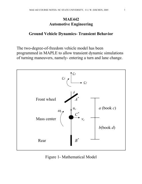
MAE 442 COURSE NOTES- NC STATE UNIVERSITY, © J. W. EISCHEN, 2005 2Bundorf Paper (see handout):1965 Ford Galaxie 2drData:M C =150 slugs=4830 lbI C =4000 slug-ft 2a=5 ftb=5 ftC αf =6250 lb/rad per tireC αr =6250 lb/rad per tire (N.S.) 12,500 lb/rad (U.S.)u c =65 MPH=95.33 ft/sec1.) Entering a turn maneuverHere the steer angle is input as a step function in time,δ=0.71 deg= 0.01239rad.

MAE 442 COURSE NOTES- NC STATE UNIVERSITY, © J. W. EISCHEN, 2005 6omegac(t),D(omegac)(t)=(-aa*Caf*(beta(t)+aa*omegac(t)/uc-str)+bb*Car*(beta(t)-bb*omegac(t)/uc))/(Ic);> init:=beta(0)=0,omegac(0)=0;> with(plots):>sol:=dsolve({sys,init},{beta(t),omegac(t)},type=numeric);> sol[2](10);Plots of Yaw Velocity and Lateral Acceleration: (plot labels can be edited)>odeplot(sol,[t,(180/3.14159)*omegac(t)],0..10,labels=[`t (sec)`,`w_c (deg/sec)`],title=`Yaw Velocity (baselinenuetralsteercar)`,font=[times,roman,16],titlefont=[times,roman,18]);

MAE 442 COURSE NOTES- NC STATE UNIVERSITY, © J. W. EISCHEN, 2005 8Next, let’s look at an understeer setup that will result in a steadystate yaw rate that is consistent a dramatically larger thanexpected turning radius. Understeer is the result of increasingthe rear tire cornering stiffness (this actually accounts for rollinducedundersteer present in most vehicles).uc= 95.33 ft/sec ⎫⎬ωc= 0.032 rad/sec⎭understeer car, results from simulationuc95.33R= = = 3009 ft (>807 ft)ω 0.032c

MAE 442 COURSE NOTES- NC STATE UNIVERSITY, © J. W. EISCHEN, 2005 9MAE 442 Automotive Engineering- Vehicle Dynamics- J. W. Eischen, March2005Two-Degree of Free Vehicle Model (bicycle model)Prediction of Lateral Velocity/Acceleration and Yaw Rate Due to Step Steer Input(entering curve maneuver)(δ=0.71 deg for t>0)Input vehicle mass and yaw moment of inertia> Mc:=150;Ic:=4000;Input distances from CG to front and rear axles, respectively> aa:=5; bb:=5;Insert front and rear tire cornering stiffness values (total)> Caf:=2*6250;Car:=2*12500;Insert forward velocity> uc:=65*5280/3600;Insert steering angle input> str:=0.71*3.14159/180;Equations of Motion and Initial Conditions:> sys:=D(beta)(t)=(-Caf*(beta(t)+aa*omegac(t)/uc-str)-Car*(beta(t)-bb*omegac(t)/uc))/(Mc*uc)-omegac(t),D(omegac)(t)=(-aa*Caf*(beta(t)+aa*omegac(t)/uc-str)+bb*Car*(beta(t)-bb*omegac(t)/uc))/(Ic);

MAE 442 COURSE NOTES- NC STATE UNIVERSITY, © J. W. EISCHEN, 2005 10> init:=beta(0)=0,omegac(0)=0;> with(plots):>sol:=dsolve({sys,init},{beta(t),omegac(t)},type=numeric);> sol[2](10);Plots of Yaw Velocity and Lateral Acceleration: (plot labels can be edited)>odeplot(sol,[t,(180/3.14159)*omegac(t)],0..10,labels=[`t (sec)`,`w_c (deg/sec)`],title=`Yaw Velocity (baselineundersteercar)`,font=[times,roman,16],titlefont=[times,roman,18]);

MAE 442 COURSE NOTES- NC STATE UNIVERSITY, © J. W. EISCHEN, 2005 11‣ odeplot(sol,[t,uc*((-Caf*(beta(t)+aa*omegac(t)/uc-str)-Car*(beta(t)-bb*omegac(t)/uc))/(Mc*uc)-omegac(t)+omegac(t))],0..10,labels=[`t(sec)`,`a_lat (ft/sec^2)`],title=`Lateralacceleration (baseline understeercar)`,font=[times,roman,16],titlefont=[times,roman,18])‣ ;

MAE 442 COURSE NOTES- NC STATE UNIVERSITY, © J. W. EISCHEN, 2005 121.) Lane change maneuverHere the steer angle is input as sinusoidal function of time,πtδ ( t) = 0.71sin( ) deg. for 0 ≤t≤8sec4= 0 for t ≥8 sec

MAE 442 COURSE NOTES- NC STATE UNIVERSITY, © J. W. EISCHEN, 2005 13δ(t)0.71 deg.4 sec 8 sect-0.71 deg.Figure 4- Ramp/Deramp Steer InputThe vehicle traverses from a straight line path to another straightline path. The yaw velocity and lateral acceleration are zero atthe end of the maneuver.

MAE 442 COURSE NOTES- NC STATE UNIVERSITY, © J. W. EISCHEN, 2005 14`u cu cFigure 5- Vehicle Path, Lane Change ManeuverNow, let’s look at the MAPLE simulation results for neutralsteer setup.MAE 442 Automotive Engineering- Vehicle Dynamics- J. W. Eischen, March2006Two-Degree of Free Vehicle Model (bicycle model)Prediction of Lateral Velocity/Acceleration and Yaw Rate Due to Ramp SteerInput (lane change maneuver)(δ=0.71*sin(Pi*t/4) deg. for 0

MAE 442 COURSE NOTES- NC STATE UNIVERSITY, © J. W. EISCHEN, 2005 15Input distances from CG to front and rear axles, respectively> aa:=5; bb:=5;Insert front and rear tire cornering stiffness values (total)> Caf:=2*6250;Car:=2*6250;Insert forward velocity> uc:=65*5280/3600;> readlib(Heaviside);> with(plots):Insert steering angle input> str:=0.71*(3.14159/180)*sin(3.14159*t/4)*Heaviside(t-0.00001)-0.71*(3.14159/180)*sin(3.14159*t/4)*Heaviside(t-8);Equations of Motion and Initial Conditions:> sys:=D(beta)(t)=(-Caf*(beta(t)+aa*omegac(t)/uc-str)-Car*(beta(t)-bb*omegac(t)/uc))/(Mc*uc)-omegac(t),D(omegac)(t)=(-aa*Caf*(beta(t)+aa*omegac(t)/ucstr)+bb*Car*(beta(t)-bb*omegac(t)/uc))/(Ic);> init:=beta(0)=0,omegac(0)=0;

MAE 442 COURSE NOTES- NC STATE UNIVERSITY, © J. W. EISCHEN, 2005 16>>sol:=dsolve({sys,init},{beta(t),omegac(t)},type=numeric);> sol[2](20);Plots of Yaw Velocity and Lateral Acceleration: (plot labels can be edited)>odeplot(sol,[t,(180/3.14159)*omegac(t)],0..20,labels=[`t (sec)`,`w_c (deg/sec)`],title=`Yaw Velocity (baselinenuetralsteercar)`,font=[times,roman,16],titlefont=[times,roman,18]);

MAE 442 COURSE NOTES- NC STATE UNIVERSITY, © J. W. EISCHEN, 2005 17> odeplot(sol,[t,uc*((-Caf*(beta(t)+aa*omegac(t)/uc-str)-Car*(beta(t)-bb*omegac(t)/uc))/(Mc*uc)-omegac(t)+omegac(t))],0..20,labels=[`t (sec)`,`a_lat(ft/sec^2)`],title=`Lateral acceleration (baselinenuetralsteercar)`,font=[times,roman,16],titlefont=[times,roman,18]);Up to now we haven’t looked at the effects of an oversteersetup. In this case the front tire cornering stiffness is higher thanthe rear and the car assumes a turning radius that is tighter thanthat predicted by the steer angle (Ackerman steering). Thefollowing plots show results for step steer input with C αf =7600deg/rad and C αr =6250 deg/rad are predicted by MAPLE. Note

MAE 442 COURSE NOTES- NC STATE UNIVERSITY, © J. W. EISCHEN, 2005 18the extremely high steady state yaw rate of approximately 16deg/sec. You can calculate the corresponding turning radius.This can lead to instability (spin-out). If the front tire corneringstiffness is increased sufficiently, the response is anexponentially increasing yaw rate.

MAE 442 COURSE NOTES- NC STATE UNIVERSITY, © J. W. EISCHEN, 2005 19Videos:Really Simple:http://youtube.com/watch?v=N9eEBnJRxtcFormula 1:http://www.youtube.com/watch?v=gn3kaLpeon8Humor: (understeer dog)http://www.autoblog.com/2006/12/01/video-audi-a4-quattro-vsthe-dog/Understeer: (dead link now)

MAE 442 COURSE NOTES- NC STATE UNIVERSITY, © J. W. EISCHEN, 2005 20http://www.esceducation.org/about_esc/how_esc_works/understeer.shtmlOversteer: (dead link now)http://www.esceducation.org/about_esc/how_esc_works/oversteer.shtmlLinks:http://www.bbc.co.uk/dna/h2g2/A1075547http://www.timskelton.com/lightning/race_prep/suspension/corrections.htm

MAE 442 COURSE NOTES- NC STATE UNIVERSITY, © J. W. EISCHEN, 2005 21MAPLE Instructions:1.) The MAPLE worksheets and all results have been producedusing MAPLE Version 10.0 (not classic or comma or mintversion).2.) You can download (by right-clicking and saving) the stepsteer (MAE442StepSteer.mw) and/or ramp steer(MAE442RampSteer.mw) programs off handouts section on theclass website.http://www.mae.ncsu.edu/courses/mae442/gould/index.html3.) If you choose to run MAPLE locally, just start theapplication and open either of the .mw worksheets. You can editany of the data entered in red. You can adjust any of the vehicleor plot parameters. After you edit parameters you must executethe worksheet by clicking on the !!! button or selecting Edit-Execute-Worksheet. This will execute the worksheet andproduce new plots that correspond to your input.4.) If you choose to run MAPLE 1-.0 remotely, typeadd maplexmaple &to the command prompt. This will start the application and thenproceed as above.