Packed Bed flooding.pdf - Youngstown State University's Personal ...
Packed Bed flooding.pdf - Youngstown State University's Personal ...
Packed Bed flooding.pdf - Youngstown State University's Personal ...

You also want an ePaper? Increase the reach of your titles
YUMPU automatically turns print PDFs into web optimized ePapers that Google loves.
14-90 EQUIPMENT FOR DISTILLATION, GAS ABSORPTION, PHASE DISPERSION, AND PHASE SEPARATION<br />
Equation (14-182) says that the backcalculated NG is 2:<br />
NG =−ln(1 − 0.86) = 2<br />
For diffusing gases of similar molecular weight, the properties that control<br />
heat transfer follow the same rules as those that control mass transfer. As a<br />
result, the NH3 scrubbing and gas cooling processes achieve similar approaches<br />
to equilibrium.<br />
For an entry temperature of 120°C and an adiabatic saturation temperature<br />
of 70°C, the expected outlet temperature would be<br />
70 + (1 − 0.86)(120 − 70) = 77°C<br />
This looks like a powerful concept, but its value is limited due to uncertainty<br />
in estimating hGa. Both h G and a are difficult to estimate due to<br />
dependence on power dissipation as discussed below. The primary<br />
value of the N G concept is in estimating an expected change from baseline<br />
data as in the comparison of Example 19 with Example 20.<br />
Example 20: A Contactor That Is Twice as Long, No Bypassing<br />
If we double the length of the pipeline contactor, double the effective<br />
contact area, and double the number of transfer units to 4, what do we expect<br />
for performance?<br />
For NG = 4,<br />
E = 1 − e−4 = 0.982<br />
The NH3 in the exit gas would be expected to drop to<br />
(1 − 0.982)(1000) = 18 ppm<br />
and the expected outlet temperature would be<br />
70 + (1 − 0.982)(120 − 70) = 70.9°C<br />
If we double the length again, we increase the number of transfer units to 8 and<br />
achieve an approach of<br />
E = 1 − e −8 = 0.9997<br />
The outlet temperature would be<br />
70 + (1 − 0.9997)(120 − 70) = 70.015°C<br />
Similarly the NH3 in the exit gas would be<br />
(1 − 0.9997)(1000) = 0.3 ppm<br />
Note that this approximates the exit condition of Example 17.<br />
Transfer Coefficient—Impact of Droplet Size The transfer<br />
coefficients increase as the size of droplets decreases. This is so<br />
because the transfer process is easier if it only has to move mass or<br />
heat a shorter distance (i.e., as the bubble or droplet gets smaller).<br />
In the limiting case of quiescent small bubbles or droplets, the<br />
transfer coefficients vary inversely with average bubble or droplet<br />
diameter. For example, in heat transfer from a droplet interface to a<br />
gas, the minimum value is<br />
hG,min = heat transfer coefficient from interface to gas = 2kG/D<br />
(14-183)<br />
where kG = gas thermal conductivity and<br />
D = droplet diameter.<br />
IMPORTANCE OF TURBULENCE<br />
The designer usually has control over the size of a droplet. As discussed<br />
below, several of the correlations show that droplet diameter<br />
varies with turbulent energy dissipation. For example, Eqs. (14-190)<br />
and (14-201) suggest that in droplet systems<br />
D ∝ {1/(gas velocity)] 1.2<br />
and hence from Eq. (14-178)<br />
a ∝ 1/D ∝ (gas velocity) 1.2 (14-184)<br />
However, just looking at the impact of velocity on droplet size underestimates<br />
the velocity impact because turbulence gives higher transfer<br />
than Eq. (14-183) predicts. Transfer coefficients increase as the mixing<br />
adjacent to the surface increases. This mixing depends on the<br />
energy dissipated into the phases. To a first approximation this transfer<br />
from droplets increases with local power dissipation raised to the<br />
0.2 power.<br />
h G,turbulent ∝ (power dissipated) 0.2<br />
and since power dissipation per unit volume increases with (velocity) 3 ,<br />
h G,turbulent ∝ (velocity) 0.6 (14-185)<br />
The combined effect on interfacial area and on the transfer coefficient<br />
is that the effective transfer increases greatly with gas velocity. From<br />
Eqs. (14-178) and (14-185)<br />
h Ga turbulent ∝ (velocity) 1.8 (14-186)<br />
For quenching operations, this means that even though residence<br />
time is cut as gas velocity goes up, the effective approach to equilibrium<br />
increases. Since the volume for a given length of pipe falls with<br />
(velocity) −1 , the expected number of transfer units NG in a given length<br />
of pipe increases with (velocity) 0.8 .<br />
See Example 21.<br />
NG,turbulent ∝ (hGaturbulent)(volume) ∝ (velocity) 0.8 (14-187)<br />
EXAMPLES OF CONTACTORS<br />
High-Velocity Pipeline Contactors High-velocity cocurrent<br />
flow can give more power input than any other approach. This is<br />
critical when extremely high rates of reaction quenching are<br />
needed.<br />
Example 21: Doubling the Velocity in a Horizontal Pipeline<br />
Contactor—Impact on Effective Heat Transfer Velocity in pipeline<br />
quench systems often exceeds 62 m/s (200 ft/s). Note that this is far above the<br />
<strong>flooding</strong> velocity in distillation packing, distillation trays, or gas-sparged reactors.<br />
There are few data available to validate performance even though liquid<br />
injection into high-velocity gas streams has been historically used in quenching<br />
reactor effluent systems. However, the designer knows the directional impact of<br />
parameters as given by Eq. (14-187).<br />
For example, if a 10-ft length of pipe gives a 90 percent approach to equilibrium<br />
in a quench operation, Eq. (14-182) says that the backcalculated NG is<br />
2.303:<br />
NG −ln(1 − 0.9) =2.303<br />
Equation (14-187) says if we double velocity but retain the same length, we<br />
would expect an increase of NG to 4.0.<br />
NG = 2.303(2) 0.8 = 4<br />
and<br />
E = 1 − e−4 = 0.982<br />
Restated, the approach to equilibrium rises from 90 percent to greater than 98<br />
percent even though the contact time is cut in half.<br />
Vertical Reverse Jet Contactor A surprisingly effective<br />
modification of the liquid injection quench concept is to inject the<br />
liquid countercurrent upward into a gas flowing downward, with<br />
the gas velocity at some multiple of the <strong>flooding</strong> velocity defined<br />
by Eq. (14-203). The reverse jet contactor can be envisioned as an<br />
upside-down distillation tray. For large gas volumes, multiple<br />
injection nozzles are used. One advantage of this configuration is<br />
that it minimizes the chance of liquid or gas bypassing. Another<br />
advantage is that it operates in the froth region which generates<br />
greater area per unit volume than the higher-velocity cocurrent<br />
pipeline quench.<br />
The concept was first outlined in U.S. Patent 3,803,805 (1974) and<br />
was amplified in U.S. Patent 6,339,169 (2002). The 1974 patent presents<br />
data which clarify that the key power input is from the gas stream.<br />
A more recent article discusses use of the reverse jet in refinery offgas<br />
scrubbing for removal of both SO 2 and small particles [Hydrocarbon