Application of Magnetic Resonance Soundings and Other ... - IWRA

APPLICATION OF MAGNETIC RESONANCE SOUNDINGS FORHYDROSTRATIGRAPHIC CHARACTERIZATION OF AN ALLUVIALAQUIFER FOR GROUND-WATER MODEL INPUTSachin D. Shah and Wade H. KressU.S. Geological SurveyTexas Water Science Center8027 Exchange DriveAustin, Texas, USA 78754email: sdshah@usgs.gov and wkress@usgs.govAnatoly LegchenkoInstitut de Recherche pour le Développement (IRD-LTHE)LTHE, BP53, 38041Grenoble Cedex 9, Franceemail: anatoli.legtchenko@hmg.inpg.frABSTRACTAn integrated surface geophysical pilot study at the Texas A&M University Brazos River HydrologicField Research Site (BRHFRS), College Station, Texas, was done to determine the effectiveness of methods fordefining the hydrostratigraphic framework and hydrogeologic properties for a ground-water availability model.Time-domain electromagnetic (TDEM) soundings and direct-current (2D–DC) resistivity imaging were used todefine the lateral and vertical extent of the Brazos River alluvium aquifer, the Ships clay within the aquifer, andthe Yegua Formation underlying the aquifer at the BRHFRS. Magnetic resonance soundings (MRS) were used toderive estimates of hydrogeologic properties including percentage water content, transmissivity, and hydraulicconductivity. Stratigraphically, the principal finding of this study was the relation between electrical resistivityand the depth and thickness of the subsurface geologic units at the site. Not only could thicknesses and extents ofthese units be defined to a greater level than previously interpreted, but lateral variations in resistivity within thealluvium aquifer also could be detected. MRS data have added supporting data to the 2D–DC resistivity andTDEM data allowing for improved understanding of the hydrostratigraphic framework. Hydrostratigraphically,individual hydraulic conductivity values derived from MRS were in close agreement with previously conductedaquifer tests. Average hydraulic conductivity values from the aquifer test are about 61 to 80 m/d, whereas, theMRS-derived hydraulic conductivity values are about 27 to 97 m/d. Results from the geophysics studydemonstrated the usefulness of combined TDEM, 2D–DC resistivity, and MRS methods to reduce the need foradditional boreholes and to create more accurate ground-water availability models using the acquired data.INTRODUCTIONThe Brazos River alluvium aquifer is used primarily as a source of supply for drinking water andagriculture in Texas and is defined by the Texas Water Development Board (TWDB) as a minor aquifer(Ashworth and Hopkins, 1995). A projected doubling of the Texas population by 2050, as well as the constantthreat of drought, necessitates the development of effective water-management plans and requires accuratecharacterization of both the geology and hydrostratigraphy of the aquifer. A ground-water availability model(GAM) for the Brazos River alluvium aquifer needs valid hydraulic conductivity, transmissivity, storagecoefficients, and other properties to simulate changes in water levels in the aquifer due to pumping and droughtconditions. The GAM includes information on hydrostratigraphic characteristics such as hydraulic conductivity,specific capacity, and transmissivity (Shah and Houston, 2007); however, numerous data gaps exist throughoutthe extent of the aquifer and require collection of additional information on the aquifer.In July 2006, the U.S. Geological Survey (USGS), in cooperation with the TWDB, did an integratedgeophysical pilot study at the Texas A&M University Brazos River Hydrologic Field Research Site (BRHFRS)

near College Station, Tex. (fig. 1), using two surface geophysical methods—time-domain electromagnetic(TDEM) soundings and two-dimensional direct-current (2D–DC) resistivity imaging to estimate the thickness,extent, and lateral variation in the resistivity of the hydrostratigraphic units—the alluvium of the Brazos Riveralluvium aquifer, the Ships clay within the aquifer, and the Yegua Formation underlying the aquifer at theBRHFRS. A third method, magnetic resonance sounding (MRS), was used to estimate the hydraulic properties,specifically percentage water content, transmissivity, and hydraulic conductivity at the BRHFRS. These datawere integrated to identify the relations between the distribution of resistivity and hydraulic properties in theBrazos River alluvium aquifer and to identify hydrostratigraphic boundaries of the Ships clay, the alluvium of theBrazos River alluvium aquifer, and Yegua Formation.This paper describes the results from the MRS and other surface geophysical methods and characterizesthe hydrostratigraphy of the Brazos River alluvium aquifer. The MRS part of the pilot study was done to comparepreviously collected hydraulic conductivity data from aquifer tests in the study area with MRS-derived hydraulicconductivity data. The paper also documents an integrated surface geophysical approach in which thehydrostratigraphy of the Brazos River alluvium aquifer at the BRHFRS was interpreted from surface geophysicalmethods.HYDROGEOLOGIC SETTINGThe BRHFRS encompasses 8.5 square hectometers of the Brazos River floodplain about 15 kilometers(km) southwest of College Station and 200 meters (m) west of the Brazos River (fig. 1). The BRHFRS wasinitially established in 1993 at the Texas A&M University Research Farm to study ground-water flow andagricultural chemical transport in the Brazos River alluvium aquifer (Munster and others, 1996). Nests of wells atthe BRHFRS were installed to monitor water quality and to assess horizontal and vertical ground-water gradientsin the Brazos River alluvium aquifer.From oldest to youngest, the geologic units at the BRHFRS are the Tertiary-age Yegua Formation (fig. 2),a shale that functions as the basal confining unit of the alluvium aquifer at an average depth of about 21 m belowland surface. The Yegua Formation is overlain by the Quaternary-age Brazos River alluvium, which is dividedinto two hydrostratigraphic units—an alluvium aquifer and an upper leaky confining unit (fig. 2). The BrazosRiver alluvium aquifer is characterized by a fining-upward sequence of coarse sand and gravel at the base to finesand at the transition zone between the aquifer and the upper leaky confining unit. The upper leaky confining unit(locally named the Ships clay) varies in thickness from about 5 m in the western part of the site to 9 m near theBrazos River (Wrobleski, 1996). The transition from the Ships clay to the Brazos River alluvium aquifer isabrupt with only a 0.3- to 0.6-m transition zone consisting of a sandy clay layer (Munster and others, 1996). Thewater table in the aquifer generally is immediately below the clay at a depth of about 9 m during the summer.Nine well nests were drilled at the site to monitor ground-water flow (Munster and others, 1996). Ahydrostratigraphic section was constructed on the basis of the driller’s logs during the installation of themonitoring wells at the BRHFRS (Munster and others, 1996). Four monitoring wells constitute each well nest;the naming convention for the wells is shown in Figure 3. The well nest identifier (MWA1, 2, or 3; MWB1, 2, or3 or MWC1, 2, or 3) precedes a well number (1 through 4) for the shallowest to deepest wells. A series of aquifertests were done at the BRHFRS in 1996 to obtain hydraulic properties of the aquifer (Wrobleski, 1996). Theaverage for each well is based on multiple aquifer tests for each interval. All hydraulic conductivity data from the1996 aquifer tests were compared to the MRS-derived hydraulic conductivity data.

Figure 1: Location of the Texas A&M University Brazos River Hydrologic Field Research Site, College Station,Texas.Table 1: Summary of average hydraulic conductivity of shallow, intermediate, and deep wells for each well nestat the Brazos River Hydrologic Field Research Site, College Station, Texas.WellnestWellidentifier(shallow)AveragehydraulicconductivityWell identifier(intermediate)AveragehydraulicconductivityWellidentifier(deep)AveragehydraulicconductivityA1 MWA1-2 -- MWA1-3 -- MWA1-4 -- --A2 MWA2-2 63 MWA2-3 57 MWA2-4 55 58A3 MWA3-2 -- MWA3-3 -- MWA3-4 68 68B1 MWB1-2 66 MWB1-3 67 MWB1-4 63 65B2 MWB2-2 64 MWB2-3 65 MWB2-4 62 64B3 MWB3-2 66 MWB3-3 69 MWB3-4 -- 68C1 MWC1-2 82 MWC1-3 80 MWC1-4 79 80C2 MWC2-2 77 MWC2-3 -- MWC2-4 93 85C3 MWC3-2 73 MWC3-3 75 MWC3-4 75 74Averagehydraulicconductivityforeach wellnest

Figure 2: Conceptual hydrostratigraphic section A-A’ across the Brazos River Hydrologic Field Research Site,College Station, Texas (modified from Wrobleski, 1996).GEOPHYSICAL METHODSTDEM and 2D–DC resistivity were used to characterize the electrical stratigraphy of the BRHFRS.These methods were used to measure the thickness, extent, and lateral variation in the resistivity of thesubsurface, which could then be used to define the correlation between electrical stratigraphic units andhydrostratigraphic units. MRS was used to estimate the hydraulic properties, specifically percentage watercontent, transmissivity, and hydraulic conductivity at the BRHFRS. These data were integrated to identify therelations between the distribution of resistivity and hydraulic properties in the Brazos River alluvium aquifer andto identify hydrostratigraphic boundaries. The survey was designed so that multiple methods could be used toachieve a more comprehensive analysis of the subsurface at BRHFRS.Time-Domain Electromagnetic SoundingsFourteen TDEM sounding sites were selected to provide a uniform distribution of data to define theframework of the electrical stratigraphy across the BRHFRS (fig. 1). The Geonics Protem-47 and -57 systemsused nine 20-square-meter (m 2 ) and five 40-m 2 transmitter loops to collect the TDEM soundings (Geonics Ltd.,2005).For each sounding, the voltage data were averaged and evaluated statistically. The raw field data (voltagedata) first were checked for uncertainty by computing the standard deviation of the voltage data from each dutycycle. The raw voltage data were then averaged over each duty cycle for each gate for each frequency usingTEM2IX1D (Interpex Ltd., 2006). The data were then imported into the inverse modeling software IX1D version

3 (Interpex Ltd., 2006). Voltages with standard deviation greater than 5 percent were deleted before modeling,which eliminated data from late-time gates that yielded the highest signal-to-noise ratios. Data that deviatedseverely from the curve were deleted before inverse modeling. A smooth model consisting of 25 layers with aminimum depth of 1 m, a maximum depth of 60 to 75 m, and a starting resistivity of 10 ohm-meters (ohm-m)were used to approximate the measured resistivity points in the starting model. A simple layered-earth model wasconstructed by comparing inflections observed in the smooth model results to the number of hydrostratigraphicunits observed in the driller’s log data from the BRHFRS monitoring wells.Final root-mean square (RMS) errors from smooth model and layered-earth model inversion resultsranged from 1.15 to 6.31 percent and from 1.09 to 6.27 percent, respectively. Any sounding with an RMS errorgreater than 5 percent was given less weight than the others because of the uncertainty in the data. Inversionresults depicted a distinct electrical contrast between the Ships clay (clay), the alluvium of the Brazos Riveralluvium aquifer (sand and gravel), and the Yegua Formation (shale).Two-Dimensional Direct-Current ResistivityThe 2D–DC resistivity survey was done using the IRIS Instruments Syscal Pro system (Iris Instruments,2006) that incorporates 96 electrodes spaced 5 m apart. A 480-m 2D–DC resistivity profile was collected tomeasure the subsurface distribution of electrical properties using the dipole-dipole array. The raw field data(current and voltage data) first were checked for uncertainty by evaluating the standard deviation of the computedapparent resistivity data using Prosys II version 2.10.02 (Iris Instruments, 2006). Apparent resistivity data withstandard deviation less than 0 were removed, resulting in the removal of 92 data points related to low signal-tonoisevalues. After filtering, 10 additional data points (three on data level 1 and seven on data level 9.1) wereremoved because of a lack of data per data level (Loke, 2000). The data were then filtered by applying a movingaverage to all depth levels with a span of 10 m. The final apparent resistivity dataset was imported into the 2Dinverse modeling software RES2DINV version 3.55 (Loke, 2004). Apparent resistivity data were inverted usingthe blocky inverse modeling technique by selecting the robust constraint option in RES2DINV. After inversionthe RMS error between the measured and calculated apparent resistivity data was 2.2 percent. Generally RMSerrors less than 5-10 percent can be expected.Magnetic Resonance SoundingsBecause this was a pilot study, the MRS modeling and interpretations are preliminary. Numis PLUSmagnetic resonance equipment (Iris Instruments, 2006) was used to collect five soundings along a single profileacross the study area (fig. 1). The square-eight antenna was used to improve the signal-to-noise ratio thusminimizing the effects of nearby power lines that run parallel to the profile where four of the soundings werecollected (Legchenko and others, 2004). Because of a lack of space and increased signal-to-noise values,sounding MRS5 used a 50-m 2 square antenna to alleviate some of the high-noise measurements. The Larmorfrequency was calculated by the system on the basis of the Earth’s magnetic field in the study area and was set to2,076.9 hertz (Hz) throughout the BRHFRS. The duration of current of the pulse was set to 40 milliseconds (ms).The recording time of the receiver was set to 240 ms to ensure that the voltage decay would be recorded until thevoltage decreased below the background noise level of the area. Using these parameters, high-quality MRS datawere acquired owing to a favorable signal-to-noise ratio indicated by the low mean noise relative to the signalamplitude (fig. 3).

Figure 3: Magnetic resonance sounding (MRS) inversion results: (A) phase relative to pulse moment, (B) depthrelative to water content, (C) depth relative to hydraulic conductivity, and (D) pulse moment relative to signalamplitude with signal-to-noise indication.Prior to MRS data inversion, a matrix for each sounding site was created. The matrix was constrained bythe following model parameters: antenna type, magnetic field inclination of the study area, maximum depth ofthe matrix, resistivity of layered-earth models obtained from the TDEM data, and the calculated maximum pulsemoment (table 2). The magnetic field inclination, used in the relaxation time calculation, was calculated using thegeospatial coordinates of each sounding and was about 60 degrees for the entire study area. The maximum depthof the matrix was set at 75 m as limited by the size of the antenna loop used.

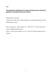
Table 2: Matrix parameters used in magnetic resonance sounding inversion, Brazos River Hydrologic FieldResearch Site, College Station, Texas.Sounding(fig. 1)AntennatypeMRS5 Square 50MRS7MRS8MRS11MRS12SquareeightSquareeightSquareeightSquareeightAntennasidelength(meters)50505050ResistivitylayerDepth tobottom oflayer(metersbelow landsurface)Resistivity(ohmmeters)1 2.80 4.502 16.70 35.303 29.50 10.104 75.00 4.201 4.30 4.102 18.10 29.403 38.10 9.604 75.00 3.001 2.70 3.202 17.60 37.603 38.20 7.504 75.00 3.001 2.80 26.702 10.10 5.103 22.70 24.304 44.50 6.905 75.00 2.701 3.30 4.802 16.40 31.803 31.60 9.004 75.00 4.20Calculatedpulse momentmaximum(amperemilliseconds)10,682.807,323.207,296.007,000.007,000.00Samovar, a program developed by Iris Instruments (2006), was used for the MRS data inversion process.Standard default parameters first were used to derive hydraulic conductivity values. However, exclusively usingthese default parameters during inversion resulted in hydraulic conductivity values that were substantially greater(5 to 10 times) than those computed from aquifer tests. Consequently, an alternate inversion method described byLegchenko and others (2004) was used.The constraints necessary for inversion include processing time, regularization parameters E (observedrelaxation time) and T1* (longitudinal relaxation time), and the coefficient of permeability (Cp). Defaultparameters maintained by the Samovar program for inversion include the processing time (198.4 ms), whichcorresponds to the Numis PLUS measurement-time window (Iris Instruments, 2006) and bandpass filter (10 Hz), Theinversion program provides the best solution for T1* on the basis of the total response of the magnetic resonancesignal.If necessary after inversion, T1* can be optimized to make the inversion solution for each sounding moredefinitive in terms of changes with depth in hydraulic conductivity, transmissivity, or signal-to-noise ratio(Legchenko and others, 2004). Using the default Cp value of 7.00 x 10 -9 assigned by the Samovar program, T1*is calibrated by running a series of inversions with different values of T1* (13 in this application) in the range of 1to 1,000. Using transmissivity as an example, the resulting transmissivity values and fitting error for eachinversion were then normalized (divided by the respective maximum). The normalized values were summed foreach inversion and graphed relative to T1* (fig. 4).

Figure 4: Calibration graph used to obtain the optimum relaxation time (T1*) for inversion of magneticresonance sounding data using the default coefficient of permeability (Cp) value of 7.00 x 10 -9 ,Brazos RiverHydrologic Field Research Site, College Station, Texas.The graph (and a similar one for each sounding) shows a curve with a flat segment corresponding to essentiallyequivalent solutions. The optimal solution is chosen to be the center of the flat segment and defined as aregularized solution that yields a value of T1* with a reasonable fitting error. The maximum, minimum, andoptimum transmissivity values for each MRS sounding are listed in table 3. The saturated thickness is thendetermined for each sounding and divided by the optimum transmissivity to yield an MRS-derived hydraulicconductivity (table 3).Table 3: Minimum, maximum, and optimal transmissivity, saturated thickness, and magnetic resonance sounding(MRS)-derived hydraulic conductivity values obtained from default coefficient of permeability (Cp) value (7.00x10 -9 ), Brazos River Hydrologic Field Research Site, College Station, Texas.Sounding(fig. 1)Minimumtransmissivity(meterssquared perday)Maximumtransmissivity(meterssquared perday)Optimumtransmissivity(meterssquared perday)Saturatedthickness(meters)MRS5 147 181 164 15 11MRS7 225 294 242 14 17MRS8 302 510 415 16 26MRS11 104 156 121 17 7MRS12 294 389 328 15 22MRS-derivedhydraulicconductivity(meters perday)

To more accurately represent the hydraulic conductivity of the soundings collected in the Brazos Riveralluvium aquifer in the study area, a Cp value that is more representative of the study area was manuallycalibrated. Data from two soundings and four monitoring well nests were used to calibrate Cp and then tocalculate hydraulic conductivity. Well nests MWB3 and MWB2 (fig. 1) correspond to MRS sounding 7 data andwell nests MWC3 and MWC2 correspond to MRS sounding 12 data. Only MRS soundings 7 and 12 were usedto calibrate Cp because of their proximity to monitoring well nests in the study area with previously obtainedhydraulic conductivity values that can be compared directly with MRS-derived hydraulic conductivity values.First, the hydraulic conductivity values obtained from the 1996 aquifer tests (Wrobleski, 1996) for well nestsMWB3 and MWB2 were combined and averaged, and then those for well nests MWC3 and MWC2 werecombined and averaged to obtain two hydraulic conductivity values (table 4).Table 4: Sounding, corresponding monitoring well nest, average hydraulic conductivity from 1996 aquifer tests,and average monitoring well nest hydraulic conductivity used to calibrate coefficient of permeability (Cp), BrazosRiver Hydrologic Field Research Site, College Station, Texas.SoundingWell nestAveragehydraulicconductivityfrom 1996aquifer test(meters per day)Well nestAveragehydraulicconductivityfrom 1996aquifer tests(meters per day)MRS7 MWB3 68 MWB2 64 66MRS12 MWC2 85 MWC3 74 80Averagemonitoringwell nesthydraulicconductivity(meters perday)Two correction factors (table 5) are then computed by dividing the average monitoring well hydraulicconductivity corresponding to MRS soundings 7 and 12 (table 4) by the MRS-derived hydraulic conductivityobtained by using the default Cp value (table 3) for both soundings. The average of these correction factors thenis multiplied by the default Cp value (7.00 x 10 -9 ) to obtain a corrected Cp value of 2.61 x10 -8 (table 5). Thecorrected Cp value is then used in the inversion.After the inversion process, a series of calculated data outputs—raw decay curves, water content,hydraulic conductivity, and signal amplitude—were generated (fig. 3). The results from MRS inverse modeling(fig. 4) can assist in estimating the percentage water content and hydraulic conductivity of the hydrostratigraphicunits. Specifically, the output data for each sounding generated from the MRS inversion include phase relative topulse moment (fig. 3A); depth relative to water content (fig. 3B); depth relative to hydraulic conductivity (fig.3C); and raw voltage decays for each signal amplitude observed in the field and best-fit line to each decay (shownin red) (fig. 3D). A final hydraulic conductivity value for each sounding based on the MRS results was derivedand compared with the previously calculated values from the 1996 aquifer tests (table 6).Table 5: Corrected coefficient of permeability (Cp) value computed using magnetic resonance sounding (MRS)-derived hydraulic conductivity from default Cp value (7.00 x 10 -9 ), average monitoring well nest hydraulicconductivity, and correction factor, Brazos River Hydrologic Field Research Site, College Station, Texas. [ a Wellnests MWB3 and MWB2; b Well nests MWC2 and MWC3]SoundingMRS-derivedhydraulicconductivity(m/d)Averagemonitoringwell nesthydraulicconductivity(m/d)CorrectionfactorAveragecorrectionfactorCorrected CpMRS7 17 66 a 3.82 3.73 2.61 x10 -8MRS12 22 80 b 3.63

Table 6: Minimum, maximum, and optimum transmissivity and magnetic resonance sounding (MRS)-derivedhydraulic conductivity values obtained from the corrected coefficient of permeability (Cp) value (2.61 x10 -8 )compared with average hydraulic conductivity values from closest monitoring well nest calculated from 1996aquifer tests, Brazos River Hydrologic Field Research Site, College Station, Texas. [ a Average for well nestsMWC2 and MWC3; about 110 meters from MRS5; b Average for well nests MWB3 and MWB2; about 20 metersfrom MRS7; c Average for well nests MWB2, MWB3, MWC2, and MWC3; about 60 meters from MRS8; dAverage for well nests MWA2 and MWA3; about 120 meters from MRS11; e Average for well nests MWC2 andMWC3; about 30 meters from MRS12]SoundingMinimumtransmissivity(m 2 /d)Maximumtransmissivity(m 2 /d)Optimumtransmissivity(m 2 /d)Saturatedthickness(m)MRS-derivedhydraulicconductivity(m/d)MRS5 548 677 612 15 40 80 aMRS7 838 1,096 902 14 64 66 bMRS8 1,128 1,901 1,547 16 97 73 cMRS11 387 580 451 17 27 61 dMRS12 1,096 1,450 1,225 15 82 80 eCONCLUSIONSAveragehydraulicconductivityfrom closestmonitoring wellnests(m/d)Prior knowledge of the general hydrostratigraphy of the alluvium of the Brazos River alluvium aquifer,the Ships clay, and Yegua Formation is required for comparison with the acquired geophysical data. Anintegrated interpretation can be made from the TDEM, 2D–DC resistivity, and MRS inversion results. Creatingthe electrical stratigraphy of the geology from TDEM and 2D–DC resistivity data and the hydrostratigraphy usingMRS data enhances the understanding of the hydrostratigraphy of the Brazos River alluvium aquifer. And MRSderivedhydraulic conductivity values can be input to ground-water availability models.Electrical Stratigraphy and Hydrostratigraphic FrameworkStratigraphically, the principal finding of this study is the relation between electrical resistivity and thedepth and thickness of the subsurface hydrostratigraphic units at BRHFRS. Not only could thicknesses andextents of these units be defined to a greater level than previously interpreted, but lateral variations in resistivitywithin the Brazos River alluvium aquifer also could be detected. The MRS soundings have added supporting datato the 2D–DC and TDEM resistivity profiles allowing for improved understanding of the hydrostratigraphicframework and the related depositional environments.The TDEM shows a three-layer model in which there is a conductor-resistor-conductor pattern. Thiscorrelates with the hydrostratigraphic units within the study area: Ships clay (conductor), alluvium of the BrazosRiver alluvium aquifer (resistor), and Yegua Formation (conductor). Sharp electrical boundaries that range from4 to 6 m and 20 to 22 m below land surface, based on the TDEM data, define the more resistive alluvium of theaquifer. The thickest part of the more resistive alluvium of the aquifer is in the middle of the study area betweenTDEM soundings BRA110 and BRA90 where the thickness is about 17 m (fig. 5C). This is interpreted to be anancestral channel deposit of the Brazos River that has not been identified previously. This interpretation is basedon correlating lithology to resistivity and comparisons of lithology to the 2D–DC and MRS soundings. The higherresistivities indicate coarse sediments (sand and gravel) shown in the driller’s logs of figures 5B and 6B.The 2D–DC resistivity profile provides a good resolution for determining lateral variation of resistivity.According to the 2D–DC resistivity profile, variations in the Brazos River alluvium aquifer range from 10 to morethan 175 ohm-m (fig. 5D). These variations are possibly caused by lateral changes in grain size and help definethe geometry of the subsurface hydrostratigraphic units (Kress and others, 2006). Resistivity increases from eastto west along the profile (fig. 5D) away from the Brazos River toward the interpreted ancestral Brazos Riverchannel. Typically, an increase in resistivity signifies an increase in grain size in the alluvium aquifer, andtherefore a more productive aquifer (more water). The highest resistivities, from about 100 to 175 ohm-m, occur

over a distance of 200 m. This zone of high resistivity (shown in blue in figure 5D) occurs between TDEMsoundings BRA110 and BRA90 and is the thickest section of coarse sediment in the ancestral channel. The zonesof lowest resistivity (or high conductivity) occur at the top of the 2D–DC resistivity profile from land surface toabout 7 m below land surface and at the base of the profile. These upper and lower zones of low resistivitycorrelate with the Ships clay and Yegua Formation, respectively. By combining TDEM and 2D–DC resistivitydata, information on the aquifer geometry and lateral variations in resistivity were obtained. These data helpedbuild the hydrostratigraphic framework into which the MRS data were integrated. Using this joint interpretationof the resistivity and MRS also helped improved the accuracy of the derived hydraulic conductivity values.HydrostratigraphyMRS data can help delineate the subsurface hydrostratigraphy and identify the geometric boundaries ofthe hydrostratigraphic units by indicating changes in the free water content, transmissivity, saturated thickness,and hydraulic conductivity (Lubczynski and Roy, 2004). Typically, this is only possible if there is a high signalto-noiseratio (fig. 3D). If the signal-to-noise ratio is too low, it might not be possible to distinguishhydrostratigraphic boundaries at depth (Lubczynski and Roy, 2004). The aquifer geometry in this applicationencompasses the lateral extent of porous and permeable materials. On the basis of the gridded MRS-derivedwater content and hydraulic conductivity data, most of the soundings show that the most productive parts of theBrazos River alluvium aquifer occur from about 15 to 20 m below land surface (fig. 6) in the western part of thestudy area and become slightly more productive in the eastern part of the area (toward the Brazos River). Theprofile indicates that the hydraulic conductivity in this productive zone is between 90 and 250 meters per day(m/d) (fig. 6D). Zones of high water content and high hydraulic conductivity occur mostly between and adjacentto MRS soundings 12 and 7 with the highest percentage water content occurring around MRS sounding 7.The higher values of water content and hydraulic conductivity are consistent with the geology based onthe TDEM and 2D–DC resistivity data in which the thickest part of the Brazos River alluvium aquifer is in themiddle of the study area. The 2D–DC resistivity data (fig. 5) show a gradual change in resistivity toward the westwhere the high resistivities indicate an increase in grain size and, therefore, a higher percentage water content andpore space. As the water content and hydraulic conductivity increase farther below land surface, coarser materialsuch as sand and gravel (Brazos River alluvium aquifer) increases.The TDEM layered models (fig. 5) and the MRS gridded water content profile (fig. 6) verify the aquifergeometry. The abrupt changes in resistivity shown in the TDEM soundings correlate with the depth and thicknessof the areas of high and low percentages of water content, particularly in the alluvium of the Brazos Riveralluvium aquifer. At most of the MRS soundings, the static water level (measured on the same day that the MRSsoundings were made) is about 10 m below land surface and therefore very little to no water (shown in yellow infigure 6C) was detected above that depth by the MRS. The minimal water detection above this depth correlateswith the compact, clay-rich material (Ships clay) above the water table. At the base of both profiles (figs. 6C and5D), percentage water content and hydraulic conductivity decrease where the Yegua Formation occurs. Verylittle or no pore space exists in that unit to hold or transmit water.Individual hydraulic conductivity values derived from MRS were consistent with those from the 1996aquifer tests. Average hydraulic conductivity values from the aquifer tests for the closest monitoring-well nestsare about 61 to 80 m/d (Wrobleski, 1996), whereas, the MRS-derived hydraulic conductivity values are about 27to 97 m/d (table 6). The highest hydraulic conductivity values indicated by the gridded hydraulic conductivityprofile are between MRS soundings 12 and 7 (fig. 6D). The alluvium aquifer is very heterogeneous in the areasof MRS soundings 5 and 11 based on MRS-derived hydraulic conductivity values that differ greatly from thesurrounding hydraulic conductivity values. MRS soundings 5 and 11 also show the greatest discrepancy betweenthe MRS-derived hydraulic conductivity and the average hydraulic conductivity computed from the 1996 aquifertests (table 6), but these soundings are farthest from the well nests. Interpreting both the gridded profiles andindividual hydraulic conductivity values derived from MRS can help generate a conceptualization of thehydrostratigraphy and constrain ground-water models for better accuracy. Collecting supporting data might benecessary to further define the hydrostratigraphy of the Brazos River alluvium aquifer at BRHFRS.

Figure 5: (A) Location of selected wells and time-domain electromagnetic (TDEM) soundings, (B) drillers’ logswith static water level, (C) TDEM layered-earth model sounding results, and (D) robust inversion profile of twodimensionaldirect-current dipole-dipole resistivity array, Brazos River Hydrologic Field Research Site, CollegeStation, Texas.

Figure 6: (A) Location of selected wells and magnetic resonance soundings (MRS), (B) drillers’ logs with staticwater-level and locations of hydraulic conductivity measurements, (C) gridded percentage water content profile,and (D) gridded hydraulic conductivity profile based on MRS results, Brazos River Hydrologic Field ResearchSite, College Station, Texas.

Hydrostratigraphic Unit ParameterizationAquifer and confining-unit properties for ground-water modeling usually are obtained from aquifer testsor calculated from known variables. However, MRS also can be used to obtain hydrostratigraphic data for inputinto ground-water models. Because of the large volume of material MRS is able to measure, properties such astransmissivity, water content, and hydraulic conductivity can be estimated over a larger area and depth, whereasaquifer tests yield data from a discreet point in the aquifer. The MRS soundings allow for many more data pointsto supplement aquifer-test sites, thus providing more comprehensive coverage of aquifer properties. In thisBrazos River alluvium aquifer study, MRS helps define the hydrostratigraphic units and vertical aquiferboundaries essential for input into ground-water models (Plata and Rubio, 2006).On the basis of historical literature, Brazos River Basin regional hydraulic conductivity ranges from about2 m/d north of the study area to about 130 m/d south of the study area (Shah and Houston, 2007). The MRS datacollected at the site are well within this range and confirm that the MRS method is capable of obtaininghydrostratigraphic unit properties at the BRHFRS. On the basis of data collected at the site, MRS could be usedin areas in the Brazos River alluvium aquifer where data are lacking and can be used in conjunction with groundwateravailability modeling. In comparison to small-scale hydrologic property measurements and expensiveaquifer tests, MRS has been shown to be an effective method to investigate large volumes of the subsurface(based on the size of the loop). For ground-water models, MRS can provide a comprehensive distribution ofproperties for model cells (Roy and Lubczynski, 2003).DisclaimerAny use of trade, product, or firm names in this paper is for descriptive purposes only and does not implyendorsement by the U.S. Government.REFERENCESAshworth, J.B., and Hopkins, Janie, 1995, Aquifers of Texas: Texas Water Development Board Report 345, 69 p.Geonics Ltd., 2005: TEM-57 transmitter: accessed August 1, 2005, at http://www.geonics.com/html/tem57-mk2.htmlInterpex Ltd., 2006: IX1D v 3 inversion software: accessed June 1, 2006, at http://www.interpex.comIris Instruments, 2006, Principles of geophysical methods for groundwater investigations: accessed August 30,2006, at http://www.iris-instruments.comKress, W.H., Ball, L.B., Teeple, A.P., and Turco, M.J., 2006, Two-dimensional direct-current resistivity surveyto supplement borehole data in ground-water models of the former Blaine Naval Ammunition Depot, Hastings,Nebraska, September 2006: U.S. Geological Survey Data Series 172, 37 p.Legchenko, A., Baltassat, J.M, Bobachev, A., Martin, C., Robain, H., and Vouillamoz, J.M., 2004, Magneticresonance sounding applied to aquifer characterization: Ground Water, v. 42, no. 3, p. 363–373.Loke, M.H., 2000, Electrical imaging surveys for environmental and engineering studies—A practical guide to 2-D and 3-D surveys: 62 p.Loke, M.H., 2004, RES2DINV version 3.55—Rapid 2D resistivity and IP inversion using the least-squaresmethod—Geoelectrical imaging 2–D and 3–D: Geotomo Software, 125 p., accessed July 12, 2007, athttp://www.geoelectrical.comLubczynski, M., and Roy, J., 2004, Magnetic resonance sounding—new method for ground water assessment:Ground Water, v. 42, no. 2, p. 291–303.

Munster, C.L., Mathewson, C.C., and Wrobleski, C.L., 1996, The Texas A&M University Brazos River hydrologicfield site: Environmental and Engineering Geoscience, v. II, no. 4, p. 517–530.Plata, J.L., and Rubio, F.M., 2006, The use of MRS in the determination of hydraulic transmissivity—The case ofalluvial aquifers: accessed June 15, 2007, athttp://www.igme.es/MRS2006/tech_program.htmRoy, J., and Lubczynski, M., 2003, The magnetic resonance sounding technique and its use for groundwaterinvestigations: Hydrogeology Journal, v. 11, no. 4, p. 455–465.Shah, S.D., and Houston, N.A., 2007, Geologic and hydrogeologic information for a geodatabase for the BrazosRiver alluvium aquifer, Bosque County to Fort Bend County, Texas: U.S. Geological Survey Open File Report2007–1031, 10 p.Wrobleski, C.L., 1996, An aquifer characterization at the Texas A&M University Brazos River hydrologic fieldsite, Burleson County, Texas: College Station, Tex., Texas A&M University, Masters thesis, 126 p.