Vegetation correlates of gibbon density in the peat ... - Vincent Nijman
Vegetation correlates of gibbon density in the peat ... - Vincent Nijman
Vegetation correlates of gibbon density in the peat ... - Vincent Nijman

Create successful ePaper yourself
Turn your PDF publications into a flip-book with our unique Google optimized e-Paper software.
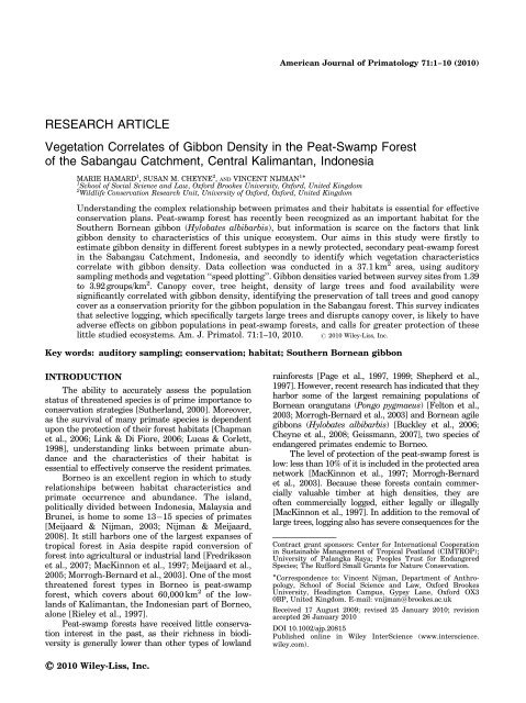
<strong>Vegetation</strong> Correlates <strong>of</strong> Gibbon Density / 3Second, because <strong>the</strong> territorial behavior <strong>of</strong> <strong>gibbon</strong>sallows efficient mapp<strong>in</strong>g <strong>of</strong> triangulated po<strong>in</strong>ts[Su<strong>the</strong>rland, 2000]. The animals’ loud calls, audiblefrom a considerable distance, allow <strong>the</strong>ir detectionfrom greater distances than by us<strong>in</strong>g sight<strong>in</strong>gs[Davies, 2002]. F<strong>in</strong>ally, fixed-po<strong>in</strong>t counts allowquick, time-efficient surveys, with more reliableresults than a l<strong>in</strong>e transect survey conducted with<strong>in</strong><strong>the</strong> same time frame [<strong>Nijman</strong> & Menken, 2005]. Thismethod has proved efficient <strong>in</strong> several primatesurveys [e.g. Brockelman & Srikosamatara, 1993;Estrada et al., 2002, 2004; Gursky, 1998; <strong>Nijman</strong>,2004] and has been used <strong>in</strong> two previous surveys at<strong>the</strong> study site [Buckley et al., 2006; Cheyne et al.,2008], allow<strong>in</strong>g <strong>the</strong> comparison <strong>of</strong> <strong>the</strong>ir results tothose yielded by <strong>the</strong> present survey.Data collection took place between 7 May and 27July 2008 at n<strong>in</strong>e sets <strong>of</strong> listen<strong>in</strong>g posts. Additionaldata were obta<strong>in</strong>ed from previous studies for two <strong>of</strong><strong>the</strong> sites with<strong>in</strong> <strong>the</strong> ma<strong>in</strong> grid system [Cheyne et al.,2008], and collected <strong>in</strong> <strong>the</strong> summer <strong>of</strong> 2007 for <strong>the</strong>two rema<strong>in</strong><strong>in</strong>g survey sites.The compass bear<strong>in</strong>gs and estimated distances <strong>of</strong><strong>gibbon</strong> calls were recorded from three listen<strong>in</strong>g postssituated <strong>in</strong> a triangle formation, with a distance <strong>of</strong> 300to 600 m between <strong>the</strong>m, for four consecutive days ateach survey site. Data collection took place between04:30 hr and 08:00 hr each morn<strong>in</strong>g exclud<strong>in</strong>g ra<strong>in</strong>ymorn<strong>in</strong>gs and morn<strong>in</strong>gs for which ra<strong>in</strong> had stopped lessthan two hours before <strong>the</strong> planned start <strong>of</strong> datacollection, as ra<strong>in</strong> has been found to <strong>in</strong>fluencenegatively <strong>the</strong> <strong>gibbon</strong>s’ s<strong>in</strong>g<strong>in</strong>g behavior [Brockelman& Ali, 1987; Brockelman & Srikosamatara, 1993].Because <strong>of</strong> this, <strong>the</strong> survey period was reduced tothree days at three <strong>of</strong> <strong>the</strong> survey sites, and two daysat one survey site. However, correction factors<strong>in</strong>cluded <strong>in</strong> <strong>the</strong> formula to estimate <strong>density</strong> ensured<strong>the</strong> data were comparable between all survey sites[Brockelman & Ali, 1987; Brockelman & Srikosamatara,1993]. Only groups for which at least one great call,<strong>in</strong>dicat<strong>in</strong>g a family group, was heard dur<strong>in</strong>g <strong>the</strong>survey time were <strong>in</strong>cluded <strong>in</strong> <strong>the</strong> analysis, <strong>in</strong> order toavoid count<strong>in</strong>g solitary animals [Brockelman & Ali,1987]. After plott<strong>in</strong>g all recorded s<strong>in</strong>g<strong>in</strong>g bouts on amap us<strong>in</strong>g Micros<strong>of</strong>t Excel, <strong>the</strong> number <strong>of</strong> groupswith<strong>in</strong> each surveyed location could be determ<strong>in</strong>edby triangulation or quadrangulation and <strong>in</strong>put <strong>in</strong>to<strong>the</strong> <strong>density</strong> formula.The <strong>density</strong> estimates (D) were obta<strong>in</strong>ed with<strong>the</strong> follow<strong>in</strong>g formula, developed by Brockelman andAli [1987]: D 5 n/[p(m) E], where n is <strong>the</strong> number<strong>of</strong> groups heard <strong>in</strong> an area as determ<strong>in</strong>ed by <strong>the</strong>mapp<strong>in</strong>g, p(m) is <strong>the</strong> estimated proportion <strong>of</strong> groupsexpected to s<strong>in</strong>g dur<strong>in</strong>g a sample period <strong>of</strong> m days,and E is <strong>the</strong> effective listen<strong>in</strong>g area. The correctionfactor p(m) was determ<strong>in</strong>ed at each site with <strong>the</strong>formula p(m) 5 1 [1 p(1)] m , with p(1) be<strong>in</strong>g <strong>the</strong>s<strong>in</strong>g<strong>in</strong>g probability for any given day, and m be<strong>in</strong>g<strong>the</strong> number <strong>of</strong> survey days. The effective listen<strong>in</strong>garea was calculated for each site us<strong>in</strong>g a fixed radius<strong>of</strong> 1 km around each listen<strong>in</strong>g post, and was def<strong>in</strong>edby <strong>the</strong> area <strong>in</strong> which at least two <strong>of</strong> <strong>the</strong> listen<strong>in</strong>gposts could hear <strong>gibbon</strong>s s<strong>in</strong>g<strong>in</strong>g. Areas which werenot covered <strong>in</strong> forest (outside <strong>the</strong> forest edges and <strong>in</strong>burnt areas) were deducted from <strong>the</strong> effectivelisten<strong>in</strong>g area us<strong>in</strong>g satellite images and GPS maps.The total survey effort covered 37.1 km 2 across <strong>the</strong>three ma<strong>in</strong> forest types, dur<strong>in</strong>g 49 survey days.Measurements <strong>of</strong> <strong>Vegetation</strong> CharacteristicsHabitat characteristics were measured <strong>in</strong> plots<strong>of</strong> 10 m 10 m situated along transects around <strong>the</strong>listen<strong>in</strong>g posts, <strong>in</strong> <strong>the</strong> same time frame as <strong>the</strong>auditory sampl<strong>in</strong>g. Previous studies <strong>in</strong>vestigat<strong>in</strong>grelationships between forest structure and primatedensities have used small plots [e.g. Blackham, 2005;Rendigs et al., 2003]. Ten plots per site wereanalyzed, with <strong>the</strong> exception <strong>of</strong> five sites with<strong>in</strong> <strong>the</strong>grid system, for which six plots per site wereanalyzed because <strong>of</strong> time constra<strong>in</strong>ts. In each plot<strong>the</strong> follow<strong>in</strong>g data were recorded: 1, canopy cover at20 m, at each corner and <strong>in</strong> <strong>the</strong> middle <strong>of</strong> <strong>the</strong> plot,us<strong>in</strong>g visual estimation by <strong>the</strong> same observerthroughout <strong>the</strong> survey; 2, diameter at breast height(DBH) <strong>of</strong> all trees exceed<strong>in</strong>g 10 cm DBH; 3, height <strong>of</strong>all trees exceed<strong>in</strong>g 10cm DBH, plac<strong>in</strong>g each tree <strong>in</strong>toclasses from 0–5 m to 35 m1 by visual estimation bytra<strong>in</strong>ed researchers; 4, local name <strong>of</strong> <strong>the</strong> species <strong>of</strong> allmeasured trees; 5, total number <strong>of</strong> trees <strong>in</strong> <strong>the</strong> plot.Additional data were obta<strong>in</strong>ed for two <strong>of</strong> <strong>the</strong> sites[Koran & Jelutong, see Fig. 2] for which 100 m 5mplots were used by ano<strong>the</strong>r team <strong>of</strong> researchers<strong>in</strong> 2007 and only DBH and tree species wererecorded. DBH was <strong>the</strong>n converted <strong>in</strong>to crosssectionalarea us<strong>in</strong>g <strong>the</strong> formula cross-sectionalarea 5 (DBH/2) 2 p and used as an <strong>in</strong>dicator <strong>of</strong> treebiomass.PCA1: vegetation characteristics210-1-2MSFtransition LIFforest typeFig. 2. <strong>Vegetation</strong> characteristics, as summarized by <strong>the</strong> pr<strong>in</strong>cipalcomponent PCA1, between forest types.TIFAm. J. Primatol.
4 / Hamard et al.All <strong>the</strong> collected data were <strong>the</strong>n summarized<strong>in</strong>to n<strong>in</strong>e variables for each plot: 1, mean canopycover; 2, median tree height; 3, mean DBH; 4,<strong>density</strong> <strong>of</strong> all trees Z10 cm DBH; 5, <strong>density</strong> <strong>of</strong> largetrees (Z20 cm DBH); 6, total cross-sectional area <strong>of</strong>all trees Z10 cm DBH; 7, total cross-sectional area <strong>of</strong>large trees (Z20 cm DBH); 8, total cross-sectionalarea <strong>of</strong> known <strong>gibbon</strong> food trees; 9, total crosssectionalarea <strong>of</strong> trees belong<strong>in</strong>g to <strong>the</strong> 20 specieseaten most frequently by <strong>gibbon</strong>s <strong>in</strong> <strong>the</strong> area. Gibbonfood trees were def<strong>in</strong>ed as tree species whose edibleparts (leaves, flowers, fruits, seeds) are known to beeaten by <strong>gibbon</strong>s <strong>in</strong> <strong>the</strong> area [Cheyne, 2008a,b;Cheyne & Sh<strong>in</strong>ta, 2006]. Tree species were identifiedby Hendri Setia Sabangau, a local field assistant wi<strong>the</strong>xtensive knowledge <strong>of</strong> forestry <strong>in</strong> <strong>the</strong> area.All vegetation characteristics were <strong>the</strong>n averagedfor each study site, except median tree heightwhich was directly calculated for all measured treeswith<strong>in</strong> a study site. Measures <strong>of</strong> species diversitywere <strong>the</strong>n added to <strong>the</strong> analysis: species richness,def<strong>in</strong>ed by <strong>the</strong> number <strong>of</strong> tree species identified <strong>in</strong>each study site; Shannon We<strong>in</strong>er’s diversity <strong>in</strong>dexand Simpson’s diversity <strong>in</strong>dex, calculated as described<strong>in</strong> Ganzhorn [2003] and Douglas [2006].Both Shannon-We<strong>in</strong>er and Simpson’s <strong>in</strong>dexes werecalculated, as both are biased towards ei<strong>the</strong>r dom<strong>in</strong>antspecies (Simpson’s <strong>in</strong>dex) or rare species(Shannon We<strong>in</strong>er <strong>in</strong>dex) [Stil<strong>in</strong>g, 2002].Statistics<strong>Vegetation</strong> characteristics between sites werecompared us<strong>in</strong>g Kruskal Wallis nonparametric test.Pair-wise comparisons <strong>of</strong> means for each <strong>of</strong> <strong>the</strong>variables were carried out between forest types us<strong>in</strong>gMann Whitney U test. After test<strong>in</strong>g for <strong>the</strong> normality<strong>of</strong> each variable us<strong>in</strong>g Kolmogorov Smirnov test,potential correlation between <strong>gibbon</strong> <strong>density</strong> andeach <strong>of</strong> <strong>the</strong> variables obta<strong>in</strong>ed from vegetationcharacteristics was <strong>in</strong>vestigated us<strong>in</strong>g Pearson’scorrelation test. A factor analysis was performed toobta<strong>in</strong> a s<strong>in</strong>gle component reta<strong>in</strong><strong>in</strong>g most <strong>of</strong> <strong>the</strong>variation conta<strong>in</strong>ed <strong>in</strong> <strong>the</strong> vegetation data set.F<strong>in</strong>ally, a l<strong>in</strong>ear regression analysis was used to test<strong>the</strong> relationship between this s<strong>in</strong>gle component and<strong>gibbon</strong> <strong>density</strong>. All tests were carried out us<strong>in</strong>g SPSSv.16, with a significance level <strong>of</strong> Po0.05. Thestandard error, which is used to assess <strong>the</strong> accuracy<strong>of</strong> calculated means <strong>in</strong> <strong>the</strong> population [Fowler et al.,1998], was used to measure variability <strong>in</strong> <strong>the</strong>analysis, ra<strong>the</strong>r than standard deviation.RESULTSCall<strong>in</strong>g Probabilities and Calculations<strong>of</strong> Gibbon DensityBased on <strong>the</strong> number <strong>of</strong> groups call<strong>in</strong>g on eachsampl<strong>in</strong>g day and <strong>the</strong> total number <strong>of</strong> groups heardfor each site, <strong>the</strong> probability for a group to be call<strong>in</strong>gon any given day p(1) was calculated. The cumulativeprobability <strong>of</strong> hear<strong>in</strong>g all <strong>gibbon</strong> groups dur<strong>in</strong>g asample period <strong>of</strong> m days, p(m), was deducted fromp(1) as described <strong>in</strong> <strong>the</strong> methods section. Table Isummarizes <strong>the</strong> parameters <strong>of</strong> call<strong>in</strong>g probabilitiesand effective listen<strong>in</strong>g areas for all survey sites, aswell as result<strong>in</strong>g <strong>gibbon</strong> <strong>density</strong> estimates.The <strong>density</strong> estimates <strong>in</strong> Table I are provided <strong>in</strong>groups per square kilometer, as no determ<strong>in</strong>ation <strong>of</strong><strong>the</strong> average group size <strong>in</strong> <strong>the</strong> area was attempteddur<strong>in</strong>g this survey. However, previous research <strong>in</strong><strong>the</strong> ma<strong>in</strong> study area has established an averagegroup size <strong>of</strong> 4.05 for <strong>gibbon</strong>s <strong>in</strong> <strong>the</strong> MSF [Cheyneet al., 2008]. Us<strong>in</strong>g this group size, <strong>the</strong> <strong>density</strong>estimate yielded by this study for <strong>the</strong> MSF is10.7070.19 <strong>in</strong>dividuals/km 2 .TABLE I. Parameters Calculated for <strong>the</strong> Estimation <strong>of</strong> Gibbon Density at Each Site, and Result<strong>in</strong>g DensityEstimatesSite name andsite numberGroups heard(N) p (1) m (days) p (m) E (km 2 )Estimated <strong>gibbon</strong><strong>density</strong> (groups/km 2 )MSF 1 5 0.67 5 1.00 1.97 2.53MSF 2 8 0.53 4 0.95 3.12 2.69MSF 3 8 0.59 4 0.97 2.78 2.96MSF 4 7 0.67 5 1.00 2.85 2.81MSF 5 7 0.64 4 0.98 2.86 2.49MSF 6 6 0.50 4 0.94 3.00 2.41MSF 7 7 0.50 4 0.94 2.86 2.61Transition 1 7 0.64 4 0.98 3.10 2.30Transition 2 5 0.55 4 0.96 3.06 1.71LIF 1 3 0.33 3 0.70 3.08 1.39LIF 2 4 0.50 2 0.75 3.13 1.70TIF 1 8 0.54 3 0.90 2.26 3.92TIF 2 8 0.54 3 0.90 3.04 2.91Reduced effective listen<strong>in</strong>g areas (E) were due to forest edges or areas <strong>of</strong> forest destroyed by wildfires. MSF: mixed-swamp forest, LIF: low <strong>in</strong>terior forest,TIF: tall <strong>in</strong>terior forest. Reduced sampl<strong>in</strong>g periods (m) were due to adverse wea<strong>the</strong>r conditions.Am. J. Primatol.
<strong>Vegetation</strong> Correlates <strong>of</strong> Gibbon Density / 5<strong>Vegetation</strong> Characteristics and Determ<strong>in</strong>ation<strong>of</strong> Forest TypesThree ma<strong>in</strong> forest types can be identified <strong>in</strong> <strong>the</strong>Sabangau <strong>peat</strong>-swamp forest: a low <strong>in</strong>terior forest(LIF) with short, small trees, a very scarce canopycover at 20 m and few large trees (Z20 cm DBH); atall <strong>in</strong>terior forest (TIF) with high, large trees, highcanopy cover and high <strong>gibbon</strong> food availability; and amixed-swamp forest (MSF), situated closest to <strong>the</strong>river, with a more heterogeneous vegetation. Twosurvey sites, situated between MSF and LIF, werelabeled transition forest. Only sites for whichvegetation <strong>in</strong>formation was obta<strong>in</strong>ed from10 10 m plots are <strong>in</strong>cluded <strong>in</strong> <strong>the</strong> calculation <strong>of</strong>species richness and diversity <strong>in</strong>dicators. A total <strong>of</strong>61 species or groups <strong>of</strong> species <strong>of</strong> trees wereidentified dur<strong>in</strong>g this study, represent<strong>in</strong>g 33 families.Overall, <strong>the</strong> vegetation <strong>in</strong> sites situated <strong>in</strong> <strong>the</strong>MSF exhibits high species richness (average s 5 27.4)and conta<strong>in</strong>s evenly distributed, relatively rarespecies (average J 5 0.92), which results <strong>in</strong> highShannon We<strong>in</strong>er <strong>in</strong>dexes (average H 5 3.04) andlow Simpson’s <strong>in</strong>dexes (average C 5 0.05). Sites <strong>in</strong>LIF exhibit poor species richness (average s 5 21)and low species diversity (average H 5 2.63; averageC 5 0.08). F<strong>in</strong>ally, TIF vegetation is species-rich(average s 5 26) but unevenly distributed (averageJ 5 0.78), with notably Palaquium leiocarpum (hangkang)trees dom<strong>in</strong>at<strong>in</strong>g <strong>in</strong> both sites and represent<strong>in</strong>g29 and 43% <strong>of</strong> <strong>the</strong> trees <strong>in</strong> sites TIF1 and TIF2,respectively. This results <strong>in</strong> a high average Simpson’s<strong>in</strong>dex (C 5 0.15) and a low Shannon We<strong>in</strong>er<strong>in</strong>dex (H 5 2.65) for TIF.All vegetation variables, averaged for each foresttype, are presented <strong>in</strong> Table II.Significant differences were found betweenforest types for all variables. Pair-wise analysisrevealed that MSF and transition forest had similarfloristic characteristics except for canopy cover,which was significantly higher <strong>in</strong> MSF (U 5 173.5,P 5 0.004). MSF also had significantly higher canopycover (U 5 72, P 5 0.01) and median tree height(U 5 189, P 5 0.01) than LIF and conta<strong>in</strong>s more <strong>of</strong><strong>the</strong> top 20 <strong>gibbon</strong> food trees (U 5 231, P 5 0.004).Canopy cover (U 5 126, P 5 0), median tree height(U 5 181.5, P 5 0.007), <strong>density</strong> <strong>of</strong> large trees(U 5 187, P 5 0), total biomass <strong>of</strong> trees (U 5 197,P 5 0.001) and large trees (U 5 189.5, P 5 0.001)were all significantly higher <strong>in</strong> TIF than <strong>in</strong> MSF, aswas total biomass <strong>of</strong> <strong>gibbon</strong> food trees (U 5 174,P 5 0.01). The biomass <strong>of</strong> <strong>the</strong> top 20 <strong>gibbon</strong> foodtrees did however not differ between TIF and MSF.Relationship between <strong>Vegetation</strong>Characteristics and Gibbon DensityAverage <strong>gibbon</strong> densities were calculated for eachforest type identified previously. The lowest <strong>gibbon</strong><strong>density</strong> was found <strong>in</strong> <strong>the</strong> LIF (1.54 groups/km 2 ),followed by <strong>the</strong> transition forest (2.00 groups/km 2 ).The average <strong>gibbon</strong> <strong>density</strong> <strong>in</strong> MSF was2.6470.07 groups/km 2 . The TIF had <strong>the</strong> highest<strong>gibbon</strong> <strong>density</strong> with 3.42 groups/km 2 . The valuesobta<strong>in</strong>ed for transition forest, LIF and TIF are<strong>in</strong>dicative values only, are <strong>the</strong> sample size is toosmall to be able to calculate a standard error.All vegetation variables had a normal distribution,as did <strong>gibbon</strong> <strong>density</strong> (Z 5 0.6, P 5 0.864 for<strong>gibbon</strong> <strong>density</strong>). Gibbon <strong>density</strong> was found to becorrelated to all <strong>the</strong> measured vegetation variables,except <strong>the</strong> <strong>density</strong> <strong>of</strong> all trees and <strong>the</strong> biomass <strong>of</strong> <strong>the</strong>top 20 <strong>gibbon</strong> food trees (Table III).Factor analysis on all vegetation variablesidentified one component, called PCA1, composed <strong>of</strong><strong>the</strong> n<strong>in</strong>e vegetation characteristics and reta<strong>in</strong><strong>in</strong>g77% <strong>of</strong> <strong>the</strong> variation <strong>in</strong> <strong>the</strong> data set. Two sites <strong>in</strong> <strong>the</strong>MSF (MSF 6 and MSF 7) were excluded from <strong>the</strong>PCA analysis because data on canopy cover and treeheight were miss<strong>in</strong>g at those sites. PCA1 allowedeasy discrim<strong>in</strong>ation between forest types (Fig. 2).The distribution <strong>of</strong> PCA1 was found to benormal (Z 5 0.577, P 5 0.893) and <strong>the</strong>re was a strongrelationship between PCA1 and <strong>gibbon</strong> <strong>density</strong>(R 2 5 0.579, P 5 0.007) (Fig. 3).TABLE II. Average <strong>Vegetation</strong> Characteristics (7SE) for <strong>the</strong> Forest Types <strong>of</strong> <strong>the</strong> Sebangau Peat-Swamp ForestForest typesMSF (n 5 42)Transition(n 5 20) LIF (n 5 20) TIF (n 5 20)Kruskal–Wallis w 2and PMean canopy cover at 20 m (%) 40.973.8 20.873.9 10.071.6 61.873.4 w 2 5 49.0; P 5 0.001Median tree height (m) 11–15 11–15 11–15 16–20 w 2 5 22.5; P 5 0.001Mean DBH (cm) 16.370.5 15.570.7 16.070.7 19.470.9 w 2 5 14.0; P 5 0.003Density large trees (trees/ha) 231.2724.9 220.0749.5 150.0728.0 385.0741.8 w 2 5 18.2; P 5 0.001CSA all trees (cm 2 ) 2,5467190 3,3327569 2,0947254 4,1987419 w 2 5 17.4; P 5 0.001CSA large trees (cm 2 ) 1,4437178 1,8527545 1,0677218 3,1047442 w 2 5 16.4; P 5 0.001CSA food trees (cm 2 ) 2,0187167 2,4697404 1,7127251 3,4557357 w 2 5 16.9; P 5 0.001CSA top20 food trees (cm 2 ) 1,0127107 1,1137200 572793 1,0377210 w 2 5 8.1; P 5 0.04CSA 5 cross sectional area. MSF 5 mixed swamp forest; LIF 5 low <strong>in</strong>terior forest; TIF 5 tall <strong>in</strong>terior forest.Am. J. Primatol.
<strong>Vegetation</strong> Correlates <strong>of</strong> Gibbon Density / 7TABLE IV. Comparison between Bornean Agile Gibbon H. albibarbis Density Estimates <strong>in</strong> Lowland and HillForest (Below 750 m above Sea Level)Density per km 2Area Forest type(s) Groups Individuals ReferenceGunung Palung Peat-swamp, Lowland, Hill 3.6 14.9 Mitani [1990]Peat-swamp 2.3 7.3 Marshall [2009]Lowland sandstone 3.4 10.3 Marshall [2009]Lowland granite 2.6 6.2 Marshall [2009]Upland granite 1.4 4.2 Marshall [2009]Tanjung Put<strong>in</strong>g Peat-swamp, lowland [2.1] a 8.7 Ma<strong>the</strong>r [1992b]Sebangau Peat-swamp (Mixed Swamp Forest) 2.2 7.5 b Buckley et al. [2006]2.6 10.7 a Cheyne et al. [2008]2.6 [10.7] a This studyPeat-swamp (Tall Interior Forest) 3.1 [12.8] a Cheyne et al. [2008]3.4 [13.9] a This studyPeat-swamp (Low Interior Forest) 1.5 [3.5] c This studyBarito Ulu Lowland [3.0] a 12 Ma<strong>the</strong>r [1992b][2.6] a 10.5 Ma<strong>the</strong>r [1992b][4.4] a 18 Ma<strong>the</strong>r [1992b][2.0] a 8.2 McConkey [2002]Estimates from Barito Ulu <strong>in</strong> italics refer to naturally occurr<strong>in</strong>g hybrids between H. albibarbis and H. muelleri. Estimates between brackets are derivedfrom <strong>the</strong> adjacent estimate us<strong>in</strong>g mean group sizes.a 4.1 <strong>in</strong>dividuals: Mitani [1990] Cheyne et al. [2008].b 3.4 <strong>in</strong>dividuals: Buckley et al. [2006].c 2.3 <strong>in</strong>dividuals: SM Cheyne [unpublished data].s<strong>in</strong>g<strong>in</strong>g can be stimulated by o<strong>the</strong>r duets fromneighbor<strong>in</strong>g groups [Brockelman & Srikosamatara,1993; Geissmann & <strong>Nijman</strong>, 2006; Mitani, 1987;<strong>Nijman</strong>, 2004]. In this study, no correlation wasfound between s<strong>in</strong>g<strong>in</strong>g probability (p(1), see Table I)and <strong>gibbon</strong> <strong>density</strong>. Gibbons s<strong>in</strong>g preferentially fromlarge, high trees [Ma<strong>the</strong>r, 1992a] and call<strong>in</strong>g probabilityhas been found to have decreased afterselective logg<strong>in</strong>g, which specifically targets thoselarge trees [Johns, 1985]. No significant correlationwas found between call<strong>in</strong>g probability and ei<strong>the</strong>r<strong>density</strong> <strong>of</strong> large trees or all vegetation characteristicsas summarized by PCA1.F<strong>in</strong>ally, as this study’s aim was to comparedensities between survey sites shar<strong>in</strong>g <strong>the</strong> samemethodology and surveyed <strong>in</strong> <strong>the</strong> same period <strong>of</strong>time, ra<strong>the</strong>r than to obta<strong>in</strong> exact <strong>density</strong> estimates,any bias associated with <strong>the</strong> method that could haveaffected <strong>the</strong> calculation <strong>of</strong> <strong>gibbon</strong> <strong>density</strong> did notaffect <strong>the</strong> subsequent comparative analysis.Habitat Characteristics and <strong>Vegetation</strong>Correlates <strong>of</strong> Gibbon DensityThe use <strong>of</strong> a large number <strong>of</strong> small plots forhabitat measurements proved efficient <strong>in</strong> this studyand allowed <strong>the</strong> detection <strong>of</strong> f<strong>in</strong>e-scale differences <strong>in</strong>vegetation characteristics. This is a time-efficientmethod that can easily be associated with auditorysampl<strong>in</strong>g, as a small number <strong>of</strong> plots can bemeasured each day after <strong>the</strong> collection <strong>of</strong> <strong>the</strong> s<strong>in</strong>g<strong>in</strong>gdata, mak<strong>in</strong>g vegetation sampl<strong>in</strong>g less fastidious andlabor-<strong>in</strong>tensive than larger plots.Gibbon <strong>density</strong> was found to be highly correlatedto vegetation parameters, <strong>in</strong> particular canopycover and tree height. As <strong>gibbon</strong>s preferentially usehigh canopy layers [Brockelman & Ali, 1987; Johns,1986; <strong>Nijman</strong>, 2001; O’Brien et al., 2004], this resultis not surpris<strong>in</strong>g, although <strong>gibbon</strong>s have proved to berelatively adaptable to disturbances <strong>of</strong> canopy coverfollow<strong>in</strong>g logg<strong>in</strong>g by shift<strong>in</strong>g <strong>the</strong>ir use <strong>of</strong> canopylayers to <strong>the</strong> lower canopy [Johns, 1985; Johns, 1986;<strong>Nijman</strong>, 2001]. Canopy cover and tree height havebeen found to <strong>in</strong>fluence <strong>the</strong> <strong>density</strong> <strong>of</strong> o<strong>the</strong>r arborealprimates [Tana River red colobus Piliocolobusrufomitratus and crested mangabey Cercocebusgaleritus: Medley, 1993; orangutans Pongo pygmaeus:Felton et al., 2003], as gaps <strong>in</strong> canopy impair<strong>the</strong>ir travell<strong>in</strong>g. O<strong>the</strong>r variables that were found tobe correlated with <strong>gibbon</strong> <strong>density</strong> <strong>in</strong> this study were<strong>the</strong> <strong>density</strong> <strong>of</strong> large trees and <strong>the</strong> availability <strong>of</strong> foodtrees. Marshall [2009] found that <strong>gibbon</strong> <strong>density</strong> wasnegatively correlated with terra<strong>in</strong> elevation atGunung Palung (West Kalimantan); <strong>the</strong> <strong>density</strong> <strong>of</strong><strong>gibbon</strong>s was highest <strong>in</strong> lowland forest which conta<strong>in</strong>edlarger trees than montane forest. Similarly,food availability for <strong>gibbon</strong>s was reduced <strong>in</strong> montaneforest where very few <strong>gibbon</strong>s were found [Marshall,2009]. Felton et al. [2003] reported a similarcorrelation between orangutan <strong>density</strong> and <strong>density</strong><strong>of</strong> large trees <strong>in</strong> a <strong>peat</strong>-swamp forest <strong>in</strong> WestKalimantan. Similar results were reported for greaterdwarf lemurs [Lehman et al., 2006] and primateAm. J. Primatol.
8 / Hamard et al.species along <strong>the</strong> Tana River [Wieczkowski, 2004].All <strong>the</strong> authors proposed that this relationship wasdue to greater availability <strong>of</strong> food where more largetrees were present, which is <strong>in</strong> conformity withresults l<strong>in</strong>k<strong>in</strong>g food abundance to primate densities[e.g. Ma<strong>the</strong>r, 1992a,b; Wieczowski, 2004]. Although<strong>the</strong> correlation between cross-sectional area <strong>of</strong> foodtrees and <strong>gibbon</strong> <strong>density</strong> was weak <strong>in</strong> this study,primarily due to large variations between plots, it issupported by <strong>the</strong> results <strong>of</strong> o<strong>the</strong>r studies on <strong>gibbon</strong>s[Marshall, 2004; Marshall & Leighton, 2006; Marshall,2009; Ma<strong>the</strong>r, 1992a], which found that <strong>gibbon</strong><strong>density</strong> was strongly <strong>in</strong>fluenced by <strong>the</strong> availability <strong>of</strong><strong>the</strong>ir preferred food trees. However, no correlationwas found between <strong>the</strong> availability <strong>of</strong> <strong>the</strong> Sabangau<strong>gibbon</strong>’s top 20 food trees and <strong>gibbon</strong> <strong>density</strong>. Thiscould be due to <strong>the</strong> fact that <strong>the</strong> list <strong>of</strong> preferred fooditems was compiled based on data from <strong>the</strong> MSFonly, and may thus not be applicable to o<strong>the</strong>r foresttypes. Alternatively, this could be due to <strong>the</strong> <strong>gibbon</strong>s’extensive range <strong>of</strong> food trees <strong>in</strong> <strong>the</strong> study area. Theirdiet <strong>in</strong>cludes at least 65 species <strong>of</strong> trees, <strong>of</strong> whichrelative importance varies seasonally [Cheyne &S<strong>in</strong>ta, 2006; Cheyne, 2008a,b], <strong>in</strong> which case a list<strong>of</strong> 20 preferred food species should be adaptedaccord<strong>in</strong>g to <strong>the</strong> months dur<strong>in</strong>g which <strong>the</strong> surveywas conducted <strong>in</strong> order to account for <strong>the</strong> animals’dietary flexibility. Gibbon <strong>density</strong> has also beenl<strong>in</strong>ked with <strong>the</strong> availability <strong>of</strong> figs, which areimportant fallback foods <strong>in</strong> many forest types[Marshall, 2004]. The correlation between <strong>the</strong> availability<strong>of</strong> figs and <strong>gibbon</strong> <strong>density</strong> was not evaluated<strong>in</strong> <strong>the</strong> present study, as phenology and feed<strong>in</strong>gecology data <strong>in</strong>dicate that fig availability andconsumption by <strong>gibbon</strong>s rema<strong>in</strong> roughly constantthroughout <strong>the</strong> year <strong>in</strong> <strong>the</strong> Sabangau <strong>peat</strong>-swampforest [Cheyne, 2008a,b]. This contrasts to o<strong>the</strong>r fieldsites with mast<strong>in</strong>g forest types, where figs areimportant food items for <strong>gibbon</strong>s <strong>in</strong> times <strong>of</strong> lowpreferred fruit availability (i.e. ripe fleshy fruit)[Marshall, 2004, 2009].Implications for ConservationThe <strong>in</strong>fluence <strong>of</strong> logg<strong>in</strong>g on <strong>gibbon</strong> populationshas been <strong>the</strong> focus <strong>of</strong> several studies [e.g. Johns,1986; Meijaard et al., 2005; Wilson & Wilson, 1975],as it constitutes a major threat to <strong>gibbon</strong>s. Selectivelogg<strong>in</strong>g, which targets large, commercially valuabletrees, has been shown to reduce canopy cover andcont<strong>in</strong>uity, as well as to restrict <strong>the</strong> availability <strong>of</strong>food for <strong>the</strong> <strong>gibbon</strong>s [Johns, 1988; Meijaard et al.,2005]. The damage on forest trees also exceeds <strong>the</strong>sole trees that are felled, as it was found thatselective removal <strong>of</strong> 3.3% <strong>of</strong> trees resulted <strong>in</strong> <strong>the</strong>destruction <strong>of</strong> over 50% <strong>of</strong> surround<strong>in</strong>g trees [Johns,1988]. Because <strong>of</strong> <strong>the</strong>ir dietary flexibility, <strong>gibbon</strong>smay be relatively resilient to logg<strong>in</strong>g: Meijaard et al.[2005] listed five studies hav<strong>in</strong>g found <strong>gibbon</strong>densities equal or higher after selective logg<strong>in</strong>g. Sixstudies cited <strong>in</strong> <strong>the</strong> same review found decreased<strong>gibbon</strong> densities after logg<strong>in</strong>g. S<strong>in</strong>ce <strong>gibbon</strong> <strong>density</strong>was highly correlated to canopy cover and treeheight, <strong>the</strong> results <strong>of</strong> this study seem to <strong>in</strong>dicatethat <strong>gibbon</strong>s <strong>in</strong> <strong>the</strong> Sabangau may have beennegatively affected by logg<strong>in</strong>g, although <strong>the</strong> populationsurvived 30 years <strong>of</strong> timber extraction <strong>in</strong> <strong>the</strong>area. Moreover, logg<strong>in</strong>g activities <strong>in</strong> <strong>the</strong> Sabangaucatchment have resulted <strong>in</strong> disruptions <strong>in</strong> <strong>the</strong>ecosystem’s hydrology, as water is dra<strong>in</strong>ed from <strong>the</strong><strong>peat</strong> by logg<strong>in</strong>g canals [Morrogh-Bernard et al.,2003]. As a result <strong>the</strong> region is prone to recurrentwildfires, which have been found <strong>in</strong> o<strong>the</strong>r tropicalsites to drastically <strong>in</strong>crease tree mortality, decreasefruit availability [Barlow & Peres, 2006; Fredrikssonet al., 2007; K<strong>in</strong>naird & O’Brien, 1998; O’Brien et al.,2003] and to affect negatively <strong>the</strong> <strong>density</strong> <strong>of</strong> largevertebrates, <strong>in</strong>clud<strong>in</strong>g siamangs, ano<strong>the</strong>r Hylobatidprimate, which are particularly vulnerable because<strong>of</strong> <strong>the</strong>ir territorial nature [O’Brien et al., 2003].This study was also designed to be used as are<strong>peat</strong> survey to monitor <strong>the</strong> <strong>gibbon</strong> population <strong>in</strong><strong>the</strong> Sabangau catchment over time. The populationseems to have rema<strong>in</strong>ed stable s<strong>in</strong>ce <strong>the</strong> start <strong>of</strong> <strong>the</strong>study period <strong>in</strong> 2004 [Buckley et al., 2006; Cheyneet al., 2008]; however, with slow-reproduc<strong>in</strong>g primatespecies such as <strong>gibbon</strong>s, population trendsrequire longer monitor<strong>in</strong>g periods to be detected, andwe hope <strong>the</strong> present survey will be followed by o<strong>the</strong>rsat this study site to detect such population trends.ACKNOWLEDGMENTSWe thank <strong>the</strong> Indonesian Institute <strong>of</strong> Science forpermission to conduct research <strong>in</strong> Sabangau forest <strong>in</strong>collaboration with <strong>the</strong> University <strong>of</strong> Palangkarayaand <strong>the</strong> Centre for International Management <strong>of</strong>Tropical Peatlands (CIMTROP) for <strong>the</strong>ir sponsorship.The research-protocols followed <strong>the</strong> AnimalBehavior Society’s Guidel<strong>in</strong>es for <strong>the</strong> Treatment <strong>of</strong>Animals <strong>in</strong> Behavioural Research and Teach<strong>in</strong>g, andwere approved by Oxford Brookes University. Fund<strong>in</strong>gwas k<strong>in</strong>dly provided by <strong>the</strong> People’s Trust <strong>of</strong>Endangered Species and <strong>the</strong> Rufford Small GrantsFoundation. This research was carried out as part <strong>of</strong><strong>the</strong> Orangutan Tropical Peatland Conservationproject and we extend our gratitude to <strong>the</strong> staff,researchers and volunteers <strong>of</strong> <strong>the</strong> OuTrop project forprovid<strong>in</strong>g advice, logistical support and assistance <strong>in</strong>data collection and analysis. Special thanks toHendri Setia Sabangau for his efficiency and hishelp dur<strong>in</strong>g <strong>the</strong> completion <strong>of</strong> this project.REFERENCESBarlow J, Peres CA. 2006. Effects <strong>of</strong> s<strong>in</strong>gle and recurrentwildfire on fruit production and large vertebrate abundance<strong>in</strong> a central Amazonian forest. Biodiversity and Conservation15:985–1012.Am. J. Primatol.
<strong>Vegetation</strong> Correlates <strong>of</strong> Gibbon Density / 9Bartlett TQ. 2007. The Hylobatidae: small apes <strong>of</strong> Asia. In:Campbell CJ, Fuentes A, K.C. M, Panger M, Bearder SK,editors. Primates <strong>in</strong> perspective. Oxford: Oxford UniversityPress. p 274–289.Blackham G. 2005. Pilot survey <strong>of</strong> nocturnal primates, Tarsiusbancanus borneanus (western tarsier) and Nycticebuscoucang menagensis (slow loris) <strong>in</strong> <strong>peat</strong> swamp forest,Central Kalimantan, Indonesia [Dissertation]. Oxford, UK:Oxford Brookes University. 59p. Available from: OxfordBrookes University.Brockelman WY, Ali R. 1987. Methods <strong>of</strong> survey<strong>in</strong>g andsampl<strong>in</strong>g forest primate populations. In: Marsh CW,Mittermeier RA, editors. Primate conservation <strong>in</strong> <strong>the</strong>tropical ra<strong>in</strong> forest. New York: Liss. p 23–62.Brockelman WY, Srikosamatara S. 1993. Estimat<strong>in</strong>g <strong>density</strong> <strong>of</strong><strong>gibbon</strong> groups by use <strong>of</strong> <strong>the</strong> loud songs. American Journal <strong>of</strong>Primatology 29:93–108.Buckley C, Nekaris KAI, Husson SJ. 2006. Survey <strong>of</strong> Hylobatesagilis albibarbis <strong>in</strong> a logged <strong>peat</strong>-swamp forest: Sabangaucatchment, Central Kalimantan. Primates 47:327–335.Chapman CA, Lawes MJ, Eeley HAC. 2006. What hope for Africanprimate diversity? African Journal <strong>of</strong> Ecology 44:116–133.Cheyne SM. 2007. Gibbon song: effects <strong>of</strong> climate, location andhuman disturbance on <strong>the</strong> s<strong>in</strong>g<strong>in</strong>g apes. American Journal<strong>of</strong> Primatology 7:1–7.Cheyne SM. 2008a. Gibbon feed<strong>in</strong>g ecology and dietcharacteristics. Folia Primatologica 79:320.Cheyne SM. 2008b. Feed<strong>in</strong>g ecology, food choice and dietcharacteristics <strong>of</strong> <strong>gibbon</strong>s <strong>in</strong> a disturbed <strong>peat</strong>-swamp forest,Indonesia. In: Lee PC, Honess P, Buchanan-Smith H,MacLarnon A, Sellers WI, editors. XXII Congress <strong>of</strong> <strong>the</strong>International Primatological Society Ed<strong>in</strong>burgh, UK, 3–8August 2008. Top Copy, Bristol. p 342.Cheyne SM. 2010. Behavioural ecology and socio-biology <strong>of</strong><strong>gibbon</strong>s (Hylobates albibarbis) <strong>in</strong> a degraded <strong>peat</strong>-swampforest. In: Supriatna J, Gursky SL, editors. Indonesianprimates. New York: Spr<strong>in</strong>ger. p 121–156.Cheyne SM, Sh<strong>in</strong>ta E. 2006. Important tree species for <strong>gibbon</strong>s<strong>in</strong> <strong>the</strong> Sabangau <strong>peat</strong> swamp forest. Report to <strong>the</strong>Indonesian Department <strong>of</strong> Forestry (PHKA), Jakarta andPalangka Raya. Palangka Raya, CIMTROP: 7.Cheyne SM, Thompson CJH, Phillips AC, Hill RMC, Lim<strong>in</strong> SH.2008. Density and population estimate <strong>of</strong> <strong>gibbon</strong>s (Hylobatesalbibarbis) <strong>in</strong> <strong>the</strong> Sabangau catchment, Central Kalimantan,Indonesia. Primates 49:50–56.Chivers DJ. 2001. The sw<strong>in</strong>g<strong>in</strong>g s<strong>in</strong>g<strong>in</strong>g apes: fight<strong>in</strong>g for foodand family <strong>in</strong> Far-East forests. Chicago. Brookfield Zoo.p 1–28.Cowlishaw G. 1992. Song function <strong>in</strong> <strong>gibbon</strong>s. Behaviour121:131–153.Davies G. 2002. Primates. In: Davies G, editor. African forestbiodiversity. Oxford: Earthwatch Press. p 99–116.Douglas PH. 2006. Microhabitat variables <strong>in</strong>fluenc<strong>in</strong>gabundance and distribution <strong>of</strong> primates (Trachypi<strong>the</strong>cusvetulus vetulus and Macaca s<strong>in</strong>ica aurifrons) <strong>in</strong> afragmented ra<strong>in</strong>forest network <strong>in</strong> southwestern Sri Lanka.[Dissertation]. Oxford Brookes University, Oxford, UK.112p.Estrada A, Castellanos L, Garcia Y, Franco B, Munoz D,Ibarra A, Rivera A, Fuentes E, Jimenez C. 2002. Survey<strong>of</strong> <strong>the</strong> black howler monkey, Alouatta Pigra, population at<strong>the</strong> Mayan Site <strong>of</strong> Palenque, Chiapas, Mexico. Primates43:51–58.Estrada A, Luecke L, Van Belle S, Barrueta E, Meda MR. 2004.Survey <strong>of</strong> black howler (Alouatta pigra) and spider (Atelesge<strong>of</strong>froyi) monkeys <strong>in</strong> <strong>the</strong> Mayan sites <strong>of</strong> Calakmul andYaxchilan, Mexico and Tikal, Guatemala. Primates 45:33–39.Felton AM, Engstrom LM, Felton A, Knott CD. 2003. Orangutanpopulation <strong>density</strong>, forest structure and fruit availability<strong>in</strong> hand-logged and unlogged <strong>peat</strong> swamp forests <strong>in</strong>West Kalimantan, Indonesia. Biology and Conservation114:91–101.Fowler J, Cohen L, Jarvis P. 1998. Practical statistics for fieldbiology. New York: Wiley. 324p.Fredriksson GM, Danielsen JE, Swenson JE. 2007. Impacts <strong>of</strong>El Niño related drought and forest fires on sun bear fruitresources <strong>in</strong> lowland dipterocarp forest <strong>of</strong> East Borneo.Biodiversity and Conservation 16:1823–1838.Ganzhorn JU. 2003. Habitat description and phenology. In:Setchell JM, Curtis DJ, editors. Field and laboratorymethods <strong>in</strong> primatology. Cambridge: Cambridge UniversityPress. p 40–56.Geissmann T. 2007. Status reassessment <strong>of</strong> <strong>the</strong> <strong>gibbon</strong>s:results <strong>of</strong> <strong>the</strong> Asian Primate Red List workshop 2006.Gibbon Journal 3:5–15.Geissmann T, <strong>Nijman</strong> V. 2006. Call<strong>in</strong>g <strong>of</strong> wild silvery <strong>gibbon</strong>s(Hylobates moloch) <strong>in</strong> Java (Indonesia): behavior, phylogenyand conservation. American Journal <strong>of</strong> Primatology68:1–19.Gitt<strong>in</strong>s SP. 1983. Use <strong>of</strong> <strong>the</strong> forest canopy by <strong>the</strong> agile <strong>gibbon</strong>.Folia Primatologica 40:134–144.Gursky S. 1998. Conservation status <strong>of</strong> <strong>the</strong> spectral tarsierTarsius spectrum: population <strong>density</strong> and home range size.Folia Primatologica 69:191–203.Johns AD. 1985. Differential detectability <strong>of</strong> primates betweenprimary and selectively logged habitats and implications forpopulation surveys. American Journal <strong>of</strong> Primatology8:31–36.Johns AD. 1986. Effects <strong>of</strong> selective logg<strong>in</strong>g on <strong>the</strong> behaviouralecology <strong>of</strong> West Malaysian primates. Ecology67:684–694.Johns AD. 1988. Effects <strong>of</strong> ‘‘selective’’ timber extractionon ra<strong>in</strong> forest structure and composition and someconsequences for frugivores and folivores. Biotropica 20:31–37.K<strong>in</strong>naird MF, O’Brien T. 1998. Ecological effects <strong>of</strong> wildfire onlowland ra<strong>in</strong>forest <strong>in</strong> Sumatra. Conservation Biology12:954–956.Lehman SM, Rajaonson A, Day S. 2006. Edge effects on <strong>the</strong><strong>density</strong> <strong>of</strong> Cheirogaleus major. International Journal <strong>of</strong>Primatology 27:1569–1588.Leighton DR. 1987. Gibbons: territoriality and monogamy. In:Smuts BB, editor. Primate societies. Chicago: University <strong>of</strong>Chicago Press. p 135–145.L<strong>in</strong>k A, Di Fiore A. 2006. Seed dispersal by spider monkeysand its importance <strong>in</strong> <strong>the</strong> ma<strong>in</strong>tenance <strong>of</strong> Neotropicalra<strong>in</strong>-forest diversity. Journal <strong>of</strong> Tropical Ecology 22:235–246.Lucas PW, Corlett RT. 1998. Seed dispersal by long-tailedmacaques. American Journal <strong>of</strong> Primatology 45:29–44.MacK<strong>in</strong>non JR, MacK<strong>in</strong>non KS. 1980. Niche differentiation <strong>in</strong>a primate community. In: Chivers DJ, editor. Malayanforest primates. Ten years’ study <strong>in</strong> tropical ra<strong>in</strong>forest. NewYork: Plenum Press. p 167–190.MacK<strong>in</strong>non K, Hatta IG, Halim H, Mangalik A. 1997. Theecology <strong>of</strong> Kalimantan. Oxford: Oxford University Press.Marshall AJ. 2004. Population ecology <strong>of</strong> <strong>gibbon</strong>s and leafmonkeys across a gradient <strong>of</strong> Bornean forest types. Ph.D.Thesis, Harvard University, Cambridge, MA.Marshall AJ. 2009. Are montane forests demographic s<strong>in</strong>ksfor Bornean white-bearded <strong>gibbon</strong>s Hylobates albibarbis?Biotropica 41:247–257.Marshall AJ, Leighton M. 2006. How does food availabilitylimit <strong>the</strong> population <strong>density</strong> <strong>of</strong> white-bearded <strong>gibbon</strong>s? In:Hohmann G, Robb<strong>in</strong>s MM, Boesch C, editors. Feed<strong>in</strong>gecology <strong>in</strong> apes and o<strong>the</strong>r primates: ecological, physical andbehavioural aspects. Cambridge: Cambridge UniversityPress. p 313–335.Ma<strong>the</strong>r R. 1992a. A field study <strong>of</strong> hybrid <strong>gibbon</strong>s <strong>in</strong> CentralKalimantan, Indonesia [Dissertation]. University <strong>of</strong>Cambridge, Cambridge, UK, 221p.Am. J. Primatol.
10 / Hamard et al.Ma<strong>the</strong>r R. 1992b. Distribution and abundance <strong>of</strong> primates <strong>in</strong>Nor<strong>the</strong>rn Kalimantan Tengah: comparisons with o<strong>the</strong>rparts <strong>of</strong> Borneo, and pen<strong>in</strong>sular Malaysia. In: Ismail G,Mohamed M, Omar S, editors. Forest biology and conservation.Kota K<strong>in</strong>abalu: Sabah Foundation. p 175–189.Medley KE. 1993. Primate conservation along <strong>the</strong> Tana river,Kenya: an exam<strong>in</strong>ation <strong>of</strong> <strong>the</strong> forest habitat. Conservationand Biology 7:109–121.Meijaard E, <strong>Nijman</strong> V. 2003. Primate hotspots on Borneo:predictive value for general biodiversity and <strong>the</strong> effects <strong>of</strong>taxonomy. Conservation Biology 17:725–732.Meijaard E, Sheil D, Nasi R, Augeri D, Rosanbaum B, Iskandar D,Setyawati T, Lammert<strong>in</strong>k M, Rachmatika I, Wong A,Soehartono T, Stanley S, O’Brien T. 2005. Life after logg<strong>in</strong>g:reconcil<strong>in</strong>g wildlife forestry and production forestry <strong>in</strong>Indonesian Borneo. Bogor, Indonesia: CIFOR. 370p.Mitani JC. 1987. Territoriality and monogamy among agile<strong>gibbon</strong>s (Hylobates Agilis). Behavioral Ecology and Sociobiology20:265–269.Mitani JC. 1990. Demography <strong>of</strong> agile <strong>gibbon</strong>s (Hylobatesagilis). International Journal <strong>of</strong> Primatology 11:409–422.Morrogh-Bernard H, Husson S, Page SE, Rieley JO. 2003.Population status <strong>of</strong> <strong>the</strong> Bornean orangutan (Pongopygmaeus) <strong>in</strong> <strong>the</strong> Sabangau Peat Swamp Forest, CentralKalimantan, Indonesia. Biology and Conservation 110:141–152.<strong>Nijman</strong> V. 2001. Effect <strong>of</strong> behavioural changes due tohabitat disturbance on <strong>density</strong> estimation <strong>of</strong> ra<strong>in</strong>forest vertebrates, as illustrated by <strong>gibbon</strong>s (Primates:Hylobatidae). In: Hillegers PJM, de Longh HH, editors.The balance between biodiversity conservation and susta<strong>in</strong>ableuse <strong>of</strong> tropical ra<strong>in</strong> forests. Wagen<strong>in</strong>gen: TropenbosInternational. p 217–225.<strong>Nijman</strong> V. 2004. Conservation <strong>of</strong> <strong>the</strong> Javan <strong>gibbon</strong> Hylobatesmoloch: population estimates, local ext<strong>in</strong>ctions, and conservationpriorities. The Raffles Bullet<strong>in</strong> <strong>of</strong> Zoology 52:271–280.<strong>Nijman</strong> V, Meijaard E. 2008. Zoogeography <strong>of</strong> primates <strong>in</strong><strong>in</strong>sular Sou<strong>the</strong>ast Asia: species-area relationships and <strong>the</strong>effects <strong>of</strong> taxonomy. Contributions to Zoology 77:117–126.<strong>Nijman</strong> V, Menken SBJ. 2005. Assessment <strong>of</strong> census techniquesfor estimat<strong>in</strong>g <strong>density</strong> and biomass <strong>of</strong> <strong>gibbon</strong>s(Primates: Hylobatidae). The Raffles Bullet<strong>in</strong> <strong>of</strong> Zoology53:169–179.O’Brien TG, K<strong>in</strong>naird MF, Nurcahyo A, Prasetyan<strong>in</strong>grum M,Iqbal M. 2003. Fire, demography and persistence <strong>of</strong>siamangs (Symphalangus syndactylus: Hylobatidae) <strong>in</strong> aSumatran ra<strong>in</strong>forest. Animal Cons 6:115–121.O’Brien TG, K<strong>in</strong>naird MF, Nurcahyo A, Iqbal M, Rusmanto M.2004. Abundance and distribution <strong>of</strong> sympatric <strong>gibbon</strong>s <strong>in</strong> athreatened Sumatran ra<strong>in</strong> forest. International Journal <strong>of</strong>Primatology 25:267–284.Page SE, Rieley JO, Doody K, Hodgson S, Husson S,Jenk<strong>in</strong>s P, Morrogh-Bernard H, Otway S, Wilshaw S.1997. Biodiversity <strong>of</strong> tropical <strong>peat</strong> swamp forest: a casestudy <strong>of</strong> animal diversity <strong>in</strong> <strong>the</strong> Sungai Sabangau catchment<strong>of</strong> Central Kalimantan, Indonesia. In: Rieley JO, Page SE,editors. Tropical <strong>peat</strong>lands. Cardigan: Samara Publish<strong>in</strong>gLimited. p 231–242.Page SE, Rieley JO, Shotyk W, Weiss D. 1999. Interdependence<strong>of</strong> <strong>peat</strong> and vegetation <strong>in</strong> a tropical <strong>peat</strong> swamp forest.Philosophical Transactions <strong>of</strong> <strong>the</strong> Royal Society <strong>of</strong> London B354:1885–1897.Raemaekers JJ, Raemaekers PM, Haim<strong>of</strong>f E. 1984. Loud calls<strong>of</strong> <strong>the</strong> <strong>gibbon</strong> (Hylobates lar): repertoire, organisation andcontext. Behaviour 91:146–189.Rendigs A, Radespiel U, Wrogemann D, Zimmermann E. 2003.Relationship between microhabitat structure and distribution<strong>of</strong> mouse lemurs (Microcebus spp.) <strong>in</strong> NorthwesternMadagascar. International Journal <strong>of</strong> Primatology 24:47–62.Rieley JO, Page SE, Lim<strong>in</strong> SH, W<strong>in</strong>arti S. 1997. The <strong>peat</strong>landresource <strong>of</strong> Indonesia and <strong>the</strong> Kalimantan <strong>peat</strong> swampforest research project. In: Rieley JO, Page SE, editors.Tropical <strong>peat</strong>lands. Cardigan: Samara Publish<strong>in</strong>g Limited.p 37–44.Shepherd PA, Rieley JO, Page SE. 1997. The relationshipbetween forest structure and <strong>peat</strong> characteristics <strong>in</strong><strong>the</strong> upper catchment <strong>of</strong> <strong>the</strong> Sungai Sabangau, CentralKalimantan. In: Rieley JO, Page SE, editors. Biodiversityand susta<strong>in</strong>ability <strong>of</strong> tropical <strong>peat</strong>lands. Cardigan: SamaraPublish<strong>in</strong>g. p 191–210.Stil<strong>in</strong>g P. 2002. Ecology: <strong>the</strong>ories and applications. UpperSaddle River, NJ: Prentice Hall.Su<strong>the</strong>rland WJ. 2000. Monitor<strong>in</strong>g mammals. In: Su<strong>the</strong>rland WJ.The conservation handbook: research, management andpolicy. Oxford: Blackwell Science. p 57–59.Whitten AJ. 1982. The ecology <strong>of</strong> s<strong>in</strong>g<strong>in</strong>g <strong>in</strong> Kloss <strong>gibbon</strong>s(Hylobates klossii) on Siberut island, Indonesia. InternationalJournal <strong>of</strong> Primatology 3:33–51.Wieczkowski J. 2004. Ecological <strong>correlates</strong> <strong>of</strong> abundance <strong>in</strong> <strong>the</strong>Tana mangabey (Cercocebus galeritus). American Journal <strong>of</strong>Primatology 63:125–138.Wilson CC, Wilson WL. 1975. The <strong>in</strong>fluence <strong>of</strong> selective logg<strong>in</strong>gon primates and some o<strong>the</strong>r animals <strong>in</strong> East Kalimantan.Folia Primatologica 23:227–245.Am. J. Primatol.