The Matrix Padé Approximation in Systems of Differential ... - WSEAS

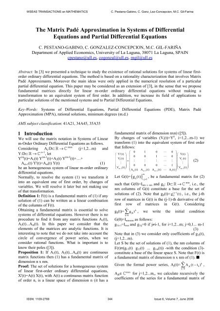
WSEAS TRANSACTIONS on MATHEMATICSC. Pestano-Gabino, C. Gonz_Lez-Concepcion, M.C. Gil-FarinaThe Matrix Padé Approximation in Systems of DifferentialEquations and Partial Differential EquationsC. PESTANO-GABINO, C. GONZΑLEZ-CONCEPCION, M.C. GIL-FARIÑADepartment of Applied Economics, University of La Laguna, 38071 La Laguna, SPAINcpestano@ull.es, cogonzal@ull.es, mgil@ull.esAbstract: In [3] we presented a technique to study the existence of rational solutions for systems of linear firstorderordinary differential equations. The method is based on a rationality characterization that involves MatrixPadé Approximants. Moreover the main ideas were only applied in the numerical resolution of a particularpartial differential equation. This paper may be considered as an extension of [3], in the sense that we proposefundamental matrices directly for linear m-order ordinary differential equations without making atransformation to an equivalent system of first order. In addition, we increase its field of applications toparticular solutions of the mentioned systems and to Partial Differential Equations.Key-Words: Systems of Differential Equations, Partial Differential Equations (PDE), Matrix PadéApproximation (MPA), rational solutions, minimum degrees (m.d.)AMS subject classification: 41A21, 34A45, 35A351 IntroductionWe will use the matrix notation in Systems of Linearm-Order Ordinary Differential Equations as follows.Considering A j :D⊂ R → C mxn (j=1,2...m) andY:D⊂ R → C n+1 , letY (m (t)=A 1 (t) Y (m-1 (t)+A 2 (t) Y (m-2 (t)+…+A m-1 (t) Y'(t)+A m (t) Y(t) (1)be an homogeneous system of linear m-order ordinarydifferential equations.Normally, to resolve the system (1) we transform itinto an equivalent one of first order, by changes ofvariables. We will resolve it later but not making useof that transformation.Definition 1: F(t) is a fundamental matrix of (1) if anysolution of (1) can be written as a linear combinationof the columns of F(t).Obtaining a fundamental matrix is essential to solvesystems of differential equations. However there is noprocedure to find it from any matrix functions A 1 (t),A 2 (t)...A m (t). In this paper we consider that theelements of the matrices are analytic functions. It isinteresting to note that we do not take into account thecircle of convergence of power series, when weconsider rational functions. What is important is toknow their poles ([3]).Proposition 1: If A 1 (t), A 2 (t)...A m (t) are continuousmatrix functions then (1) has a fundamental matrix ofdimension n x nm.Proof: The set of solutions for a homogeneous systemof linear first-order ordinary differential equations,X'(t)=A(t) X(t), with A(t) a continuous matrix functionof order n, is a linear space of dimension n (it has afundamental matrix of dimension nxn) ([5]).By changes of variables (V i (t)=Y (i , i=1,2...m-1) wetransform (1) into the equivalent system of first orderthat follows:⎛ 0 I 0 ⋯ 0 ⎞⎛ Y '(t) ⎞ ⎜⎟⎛ Y(t) ⎞⎜ 0 0 I 0' ⎟V1(t)⎜⋯ ⎟⎜ ⎟⎜ ⎟ V1(t)= ⎜ ⋮ ⋮ ⋮ ⋯ ⋮ ⎟⎜ ⎟⎜ ⋮ ⎟ ⎜⎟⎜ ⋮ ⎟⎜ ⎜ 0 0 0 I ⎟V (t) ⎟ ⋯ ⎜ V (t) ⎟⎝ ⎠ ⎝ ⎠'m−1 ⎜m−1Am(t) Am−1(t) Am−2(t) A1(t)⎟⎝⋯ ⎠g ) mij(t)i, j= 1Let G(t)= ((2), be a fundamental matrix for (2)such that G(0)=I nm x nm and g ij : D⊂ R → C nxn , i.e., thenm columns of G(t) constitute a base for the set ofsolutions of (2). Note that g ji (t)= ( j −g11i(t) , i.e., the j-throw of matrices in G(t) is the (j-1)-th derivative of thefirst row of matrices in G(t). Considering∞kg ij (t)= ∑ gijkt, we write the initial conditionk=0G(0)=I nmxnm as follows:g 1ii-1 =I nxn and g 1ij =0 if j≠i-1, for i=1,2...m; j=0,1... m-1(3)Note that in (3) we consider only coefficients of g 1j (t),(j=1,2...m).Let S be the set of solutions of (1), the nm columns ofF(t)≡(g 11 (t) g 12 (t) ... g 1m (t)) -with the condition (3)-constitute a base of the linear space S. Note that F(t) isa fundamental matrix of dimension n x nm of (1). ■kGiven the formal power series, A j (t)= ∑ Ajk(t − t0) ,∞k=0A jk ∈ C mxn for j=1,2...m,, we calculate recursively thecoefficients of the series for a fundamental matrix ofISSN: 1109-2769 344 Issue 6, Volume 7, June 2008

WSEAS TRANSACTIONS on MATHEMATICSC. Pestano-Gabino, C. Gonz_Lez-Concepcion, M.C. Gil-Farina∞k(1), F(t)= ∑ Fk(t − t0) , F k ∈ Cnxmn , as follows (withoutk=0considering the equivalent system of first-order).SubstitutingF (h (t)=∞∑k=0k(k + h)(k + h − 1)...(k + 1)F (t − t ) , h=1, 2...m,k+h 0in F (m (t)=A 1 (t)F (m-1 (t)+A 2 (t)F (m-2 (t)+ +A m-1 (t)F'(t)+A m (t)F(t). Later on, we will explain moreexplicitly the recurrence relation for the specificexamples we are going to study.2 Matrix Padé Approximants andRational FunctionsOnce the formal power series for a fundamental matrix(or for a particular solution) is obtained, it is ofpractical interest to get the theoretic functionassociated to the series. It is evident that this aim isunattainable in general and it may only be obtain incertain problems.In this section we will consider Matrix PadéApproximation (MPA) results to determine it there is arational solution and, if so, obtain minimum degrees -in certain sense- of the polynomials involved.We denote as F any formal power series, with matrixcoefficients as follows:∞kmxnF(t) = fk t fk∈ tk=0∑ C ∈C (4)Suppose that there exist matrix polynomials:Q (z) =hhi∑bizi=0hiN h(z) = ∑n iz n ii=0Pg(z) =Dg(z) =g∑i=0g∑i=0ia izidizq ∈Cip ∈Ci∈Cdi∈Cmxnmxnnxnmxmpara i = 0,1,..,hpara i = 0,1,..,hpara i = 0,1,..,gpara i = 0,1,..,gwhere p 0 =I nxn , d 0 =I mxm , F(t)-Q h (t)P -1 g (t)=O(t h+g+1 ) andF(t)-D -1 g (t)N h (t)=O(t h+g+1 ), Q h P -1 g is therefore said to bea right Matrix Padé Approximant (right MPA) which isdenoted R [h/g] F ; similarly, D -1 g N h is said to be a leftMatrix Padé Approximant (left MPA), which is denotedL [h/g] F . We shall use { L [h/g] F } ({ R [h/g] F }) to denote theset of all possible approximants L [h/g] F ( R [h/g] F ).As a consequence of the definition we can say that:* R [h/g] F exists, i.e., { R [h/g] F }≠∅, if and only if, thefollowing system has a solution:f h-g+k p g +f h-g+k+1 p g-1 +...+f h+k-1 p 1 =-f h+k , k=1,2...g RS(h,g)* L [h/g] F exists, i.e., { L [h/g] F }≠∅, if and only if thefollowing system can be solved:d g f h-g+k +d g-1 f h-g+k+1 +...+d 1 f h+k-1 =-f h+k k=1,2...g LS(h,g)In both cases it is assumed that f i =0, i0, letjM1( i, j) = ( f i− j+ h+ k− 1) h , k=1,LLM4 (i, j) = (f ) ,j,s+ r−isr i− j+ h+ k− 1 h,k=1M5 (i, j) = (f ) ,Rj+ 1,s+ r−isr i− j+ h+ k− 1 h,k=1M4 (i, j) = (f )s+ r−i,jsr i− j+ h+ k− 1 h,k=1M5 (i, j) = (f )R s+ r− i,j+1sr i− j+ h+ k− 1 h,k=1By convention, if j=0 the rank of these matrices is zerofor any i∈N.Definition 4: For any nonnegative integers i, j, letT1(i,j)=rank(M1(i,j)). We will display these quantities inan infinite two-dimensional table, Table 1, where i and jserve to enumerate the columns and the rowsrespectively.Definition 5: We define the staired block R1 to be thefollowing subset of N 2 :R1={(i,j)∈ N 2 /rank(M1(g,h))=rank(M1(g+k,h+k)) forany k∈N, g≥i and h≥j}..ISSN: 1109-2769 345 Issue 6, Volume 7, June 2008

WSEAS TRANSACTIONS on MATHEMATICSC. Pestano-Gabino, C. Gonz_Lez-Concepcion, M.C. Gil-FarinaAlthough this set seems rather abstract, the meaning of"staired" becomes clear observing Tables 1 in examplesbelow.To begin with, we can propose a method, using Table 1,to determine whether or not a matrix series stems from arational function. This can be set out as follows.2.1.1.1 RationalityF is rational if and only if in the bottom right part ofTable 1 we can mark at least one NW-SE diagonal ofinfinite size where all its boxes have the same value. It isimportant to state that, there are several such diagonals,with their union coinciding with R1. Note that, withinR1, boxes of different diagonals can have differentvalues. Furthermore, it is assured that if (a,b)∈R1 thenthe formal power series of F and [a/b] F is the same.However, (a,b) are not necessarily left or right m.d.In practice, the Table 1 that we can construct is "finite".However, in some applications where a rule for theformation of the coefficients of the series F is known,certain relations between the matrices that define theelements of Table 1 can help validate the properties toan infinite size. Otherwise, we can only say the availablecoefficients of F coincide with the coefficients of arational function of certain degrees.2.1.1.2 MinimalityThe boxes (i,j) such that T1(i,j)∈R1, T1(i-1,j)∉R1 andT1(i,j-1)∉R1 are called corners of R1. In particularsituations we can say that a corner of R1 correspondswith a pair of left or right m.d., for instance:Property 1: If (i,j)∈R1, (i-1,j)∉R1 and T1(i,j)=jn then(i-u,j-v) is not a pair of right m.d. for any u, v such that1≤u≤i and 0≤v≤j.Property 2: If (i,j)∈R1, (i-u,j)∉R1, (i,j-v)∉R1, for anyu, v such that 1≤u≤i and 1≤v≤j, and they are not pairs ofleft (right) m.d., then (i,j) is a pair of left (right) m.d.2.1.2 Table 2: MinimalityIf F is rational, there are (and we can find) certaindegrees r and s associated to two pairs of matrixpolynomials which represent the function in rationalform in two ways, that is to say, with the invertedpolynomial of degree r, multiplied to the right or left.However, it may be that r and s are neither left nor rightm.d. for representing F since there are cases in which,for instance, the function is identical to an approximantL [i/j] F but the approximant R [i/j] F does not exist, orviceversa; in this case, rank(M1(i,j))≠rank(M1(i+1,j+1))and thus Table 1 would not provide informationconcerning the left or right approximant. For this reason,we present Table 2 -one for the left and one for the rightapproximant-, whose structure reflects the possiblecombinations of m.d. (left and right, respectively) forrepresenting F.Firstly we present the following definitions.Definition 6: Given (s,r)∈R1, for integer i, j, such that0≤i≤s and 0≤j≤r, let L T2 sr (i,j)=0, if rank( L M4 sr (i,j))=rank( L M5 sr (i,j)), or otherwise L T2 sr (i,j)=1. We willdisplay these quantities in a finite two-dimensional table,Table 2 for left approximant, which has s+1 columnsand r+1 rows.Definition 7: We denote as a staired block L R2 sr , with(s,r)∈R1, the following subset of N 2 :L R2 sr ={(i,j)∈ N 2 /0≤i≤s, 0≤j≤r andrank( L M4 sr (i,j))=rank( L M5 sr (i,j))}.To define Table 2 for right approximant we mustconsider R M4 sr (i,j) and R M5 sr (i,j) instead of L M4 sr (i,j) andL M5 sr (i,j), respectively. We only expound the theory forthe left case taking into account that for the right case itis similar.Property 3: F is a rational function identical to L [q/p] Fwhere q and p are left m.d., q≤s and p≤r, if and only if,L T2 sr (q,p)=0, L T2 sr (q-1,p)=1 and L T2 sr (q,p-1)=1, that is,(q,p) is a corner of L R2 sr .The system corresponding to the denominator of theelement of { L [q/p] F } that coincides with F is:d p f q-p+i +d p-1 f q-p+i+1 +...+d 1 f q+i-1 =-f q+i i=1,2...s+r-qwhose associated matrix is L M4 sr (q,p).Then we will consider the results of MPA to studypossible rational solutions of differential equationssystems and of partial differential equations.3 Rational Solutions for Systems ofOrdinary Differential EquationsIn order to obtain a clear understanding, it is importantto read the following remarks relating to possiblerational solutions of the system (1).- Even if A 1 (t), A 2 (t)...A m (t) are not rational there mayexist rational solutions. For instance, the systemtt⎛ e − e + 2 ⎞⎜⎟Y'(t)= ⎜ 2t + 4 2t + 4 ⎟ Y(t)sint − sin t + 2⎜⎟⎝ 2t + 4 2t + 4 ⎠⎛has a rational solution, Y(t)= 2t + 4 ⎞⎜ ⎟⎝ 2t + 4.⎠- The fact that there exists rational solution does notimply the fundamental matrix is rational. Note thatgenerally the linear combination of no rationalfunctions could be a rational function, for instance, ifx(t)= cos t−and y(t)= 2cos t + 8 the linear3t − 23t − 216combination 4x(t)+2y(t) is the rational function3t − 2.- The system (1) may have a fundamental matrix withISSN: 1109-2769 346 Issue 6, Volume 7, June 2008

WSEAS TRANSACTIONS on MATHEMATICSC. Pestano-Gabino, C. Gonz_Lez-Concepcion, M.C. Gil-Farinasome rational elements and others which are not. Nextwe proceed to illustrate different cases.Our aim in this section is to detect rationalfundamental matrices (which are rectangular when theorder of the system is greater than 1). In other case, ifthis is not possible, then to detect particular rationalcolumns or particular rational solutions. If F(t) isrational then any solution of (1) is rational complyingwith the aims. However, when F(t) is not rational andis in analytical form it would be interesting to know ifthere exist any initial conditions, such that theassociated particular solution to be rational. It is noteasy to find the answer to this question in generalcases.We start with an example where the fundamentalmatrix is not rational but the system does have rationalsolutions.Example 1. Let Y''(t)=C(t) Y(t) be a differential2⎛ 1 t + 2 ⎞⎜ 2 3 ⎟(2 t) (2 t)system where C(t)= ⎜ − − ⎟ . Considering⎜24t − 8 6t ⎟⎜2 3 2 2(t + 2) (t + 2)⎟⎝⎠C(t)=∞∑i=0C tii, we obtain recursively the coefficients ofthe series for a fundamental matrix F(t)=follows:∞ ∞ ∞i i i+ +i+2=i ii= 0 i= 0 i=0∞∑i=0F tii∑(i 2)(i 1)F t ( ∑C t )( ∑ F t )(5)⎛Then, taking into account (3), F 0 = 0 0 1 0 ⎞⎜ ⎟⎝0 0 0 1and⎠⎛F 1 = 1 0 0 0 ⎞⎜ ⎟ , and considering (5) we calculate the⎝0 1 0 0⎠ other coefficients using the following expression:F i+2 =( ∑ i CjF i−j) /(i + 2)(i + 1) , i≥0 (6)j=0Fig. 1: Table 1 for F(t)0 1 2 3 4 50 0 0 0 0 0 01 2 2 2 2 2 22 4 4 4 4 4 43 6 6 6 6 6 64 8 8 8 8 8 85 10 10 10 10 10 10Note that F(t) is not rational of orders (p,q) such that0≤p

WSEAS TRANSACTIONS on MATHEMATICSC. Pestano-Gabino, C. Gonz_Lez-Concepcion, M.C. Gil-Farinaw j (x)= 2 sen πjx. In this case, the equation (10) inmatrix form is:V'(t)=A(t) V(t) (11)where V(t) = (v 1 (t) v 2 (t) ... v n (t)) t and A(t) is an nxnmatrix which elements are:3 'a ij (t)= w2 j, wi.2(4 + t )Considering the initial conditions, we have:n∑ vj(0)w j(x)= sin 2πx. Due to the fact thatj=1{w 1 ,w 2 ...w n } is an ortonormal system, then:v j (0)= sin 2π x, wj(j=1...n) (12)The expression (12) provides initial conditions forsystem (11).To illustrate the procedure, suppose that n=2 in (8).Obviously, with greater n we obtain betterapproximation.1 ⎛0 −1⎞If n=2, then A(t)=2 ⎜ ⎟t 1 0. Considering1+⎝ ⎠4A(t)=∞∑j= 0jA jtj⎛ ⎛ 1 ⎞⎜ 0 ⎜ ⎟ ( −1)4A 2j =⎜ ⎝ ⎠⎜ j⎛ −1⎞⎜⎜⎟ 0⎝⎝4 ⎠, we have that A 2j+1 =0,j+1A fundamental matrix F(t)=such that F 0 =I, verifies thatk1F k+1 = ∑ AjFk − jk≥0k + 1j=0⎞⎟⎟⎟for j=0,1,2...⎟⎠Fig. 7: Table 1 for F(t)0 1 2 3 4 50 0 0 0 0 0 01 2 2 2 2 2 22 4 4 2 2 2 23 6 6 4 2 2 24 8 8 6 4 2 25 10 10 8 6 4 2∞j∑ Fjtof the system (11)j=0It indicates that F(t)=[1/1] F . Solving the systemLS(1,1), and calculating the numerator, F(t) can berepresented as follows:⎡⎛1 0⎞ ⎛ 0 1/ 2⎞ ⎤ ⎡⎛1 0⎞ ⎛ 0 −1/ 2⎞⎤F(t) = ⎢⎜ ⎟ + ⎜ ⎟ t⎥ ⎢⎜ ⎟ + ⎜ ⎟ t⎥⎣⎝0 1⎠ ⎝ −1/ 2 0 ⎠ ⎦ ⎣⎝0 1⎠ ⎝1/ 2 0 ⎠ ⎦2⎛ t ⎞1 t1⎜ − − ⎟or equivalently F(t)= ⎜ 4 ⎟ .2 2t ⎜ t ⎟1+ t 1−4⎜⎟⎝ 4 ⎠Given initial conditions, we calculate the particular−1solution V(t)=F(t)K, where K∈ R 2 . Note that V(0)=K.⎛ 0 ⎞Taking into account (12), K=⎜1/ 2 ⎟. Therefore,⎝ ⎠⎛ −t⎞1V(t)= ⎜ 2 ⎟2 t andt 1−2(1 + ) ⎜ ⎟⎝ 4 ⎠42t−t sin π x + (1 − )sin 2πxu(x,t)=4 .2t1+4In the case that we are interested only in a particularsolution that verifies certain initial conditions, it is notnecessary to calculate a fundamental matrix. To know∞⎛ 0 ⎞jV(t), we suppose that V(t)= ∑ Vjt, with V 0 =⎜j=01/ 2 ⎟.⎝ ⎠k1Then se V k+1 = ∑ AjVk − j, k≥0.k + 1j=0Fig. 8: Table 1 for V(t)0 1 2 3 4 50 0 0 0 0 0 01 1 1 1 1 1 12 2 2 2 2 2 23 3 3 3 2 2 24 4 4 4 3 2 25 5 5 5 4 3 2This table indicates that V can be represented as leftand right approximants of the set {[2/2] V }.Considering right approximant, Table 2 is notnecessary because in Table 1 we can see taht (2,2) is apair of right m.d. (taking into account Properties 1 and2 and T1(2,2)=2). We solve the system RS(2,2) to⎛ −t / 2 ⎞⎜ ⎟ 1obtain the known solution V(t)= 2⎜ 1 t ⎟ .2⎜ − ⎟t⎝ 2 4 2 ⎠(1 + )4Out of curiosity we have calculated the Table 2 for leftapproximant in fig. 9.Fig. 9: Table 2 for left approximant0 1 20 1 1 11 1 0 02 0 0 0It indicates that (0,2) and (1,1) are two pairs of leftm.d.Let us consider the following example. In this case weneed to solve a system of first order ordinarydifferential equations, V''(t)=A(t) V(t) where A(t) is adiagonal matrix, then each equation can be solveindividually. Therefore, instead of MPA we will usescalar Padé approximation.ISSN: 1109-2769 349 Issue 6, Volume 7, June 2008

WSEAS TRANSACTIONS on MATHEMATICSC. Pestano-Gabino, C. Gonz_Lez-Concepcion, M.C. Gil-FarinaExample 4Let it be the following elliptic equation:2u tt = − u2 2 xx , t>0, t≠1, 0≤x≤1π (1 − t)u(0,t)=u(1,t)=0; u(x,0)=u t (x,0)=sinπxWe propose a solution of the form u(x,t)= 2 vj(t)w j(x)considering the same ortonormal system of Example 3.Substituting in the partial differential equation anddividing by 2 ), we obtain:'' 22v1(t)sin π x+ v2 2 1(t)( −π sin π x) +π (1−t)'' 22v2(t)sin2π x + v2 2 2(t)( −4π sin2π x) = 0π (1 −t)'' 2'' 8Then, v1(t)= v2 1(t), v2(t) = v2 2(t)(1 − t)(1 − t)We have two independent equations. Note that A(t) isa diagonal matrix.The initial conditions can be deduced by:u(x,0)=v 1 (0)w 1 (x)+v 2 (0)w 2 (x)=sin πx, therefore,v 2 (0)=0 and v 1 (0)= 1 2 ,∑j=1u t (x,0)= v ' (0)w (x) + v ' (0)w (x) = sin π x , therefore,''2 11 1 2 2v (0) = 0 and v (0) =Considering the first equation122v (t) =(1 − t)v (t)''1 2 1andits conditions v 1 (0)= 1 2 and ' 1v1(0)= , we denote2the general solution as s(t)=∞i∑ siti=0. Taking into account∞2jthat = 2 (j 1)t2 ∑ + -in the circle of convergence(1 − t) j=0of the series-. Substituting in the differential equationwe obtain:∞ ∞ ∞i i i∑ + +i+2= ∑ + ∑ ii= 0 i= 0 i=0(i 2)(i 1)s t 2( (i 1)t )( s t )Therefore, to calculate the coefficients of the series s(t)we use the following recurrence relation:is i+2 = 2( ∑ (j+ 1)si−j) /((i + 2)(i + 1)) i≥0.j=0Fig. 10: Table 1 for v 1 (t)0 1 2 3 4 50 0 0 0 0 0 01 1 1 1 1 1 12 2 1 1 1 1 13 3 2 1 1 1 14 4 3 2 1 1 15 5 4 3 2 1 1It shows that v 1 (t)=[0/1] s . Solving Padé equations for[0/1] s , v 1 (t)= 1/ 2 . In a similar way, solving1−t'' 8v2(t) = v2 2(t) , v 2 (0)= v ' 2(0) = 0 , we obtain(1 − t)v 2 (t)=0. Therefore, the solution of the partialdifferential equation is: u(x,t)= 1 sin πx.1−t4.2 Method of Finite Differences and MPAWe give the theory for the following hyperbolic partialdifferential equation (generalized wave equation):u tt =α 2 (x,t) u xx 0≤x≤1, t>0u(0,t)=f 1 (t), u(1,t)=f 2 (t); u(x,0)=g 1 (x), u t (x,0)=g 2 (x)In this method we choose n∈N, calculate h=1/n andconsider the points (x i ,t) where x i =ih for i=0,1,2...n.Note that we do not discretise variable t.Substituting these points, for i=1...n-1, we obtainu tt (x i ,t) = α 2 (x i ,t) u xx (x i ,t). If we replace second partialderivative u xx with second differences we obtain:u tt (x i ,t)=α 2 u(xi+ 1, t) − 2u(xi, t) + u(xi−1, t)(x i ,t) u2xx (x i ,t),hfor i=1...n-1Denoting2⎛ α (x1, t)f1(t)⎞⎜2 ⎟⎛ u(x1, t) ⎞ ⎜ h ⎟⎜ ⎟ ⎜ 0 ⎟u(x2, t)Y(t)= ⎜ ⎟ ⎜⎟, b(t)=⎜ ⋮ ⎟ ⎜⋮⎟and⎜ ⎟ ⎜ 0 ⎟⎝ u(xn−1, t) ⎠ ⎜⎟2α (xn−1, t)f2(t)⎜2 ⎟⎝ h ⎠2 2⎛−2 α (x,t)1α (x,t)10 ⋯ 0 ⎞⎜ 2 2 2⎟(x2,t) 2 (x2,t) (x2,t) 01⎜ α − α α ⋯⎟2 2A(t)= ⎜20 α (x3,t) −2 α(x 3,t) ⋯ 0 ⎟,h ⎜⎟⎜ ⋯ ⋯ ⋯ ⋯ ⋯ ⎟⎜2 20 0 α (xn−1 ,t) −2 α (xn−1,t) ⎟⎝⋯⎠we obtain the system of linear second-order ordinarydifferential equations:Y''(t)=A(t) Y(t)+b(t) (13)Note that the solution vector Y(t) is of dimension n-1.The initial conditions for this system are:⎛ g1(x 1)⎞ ⎛ g2(x1)⎞⎜ ⎟ ⎜ ⎟g1(x 2)Y(0)= ⎜ ⎟ , Y'(0)= ⎜g2(x2)⎟⎜ ⋮ ⎟ ⎜ ⋮ ⎟⎜ ⎟ ⎜ ⎟⎝g 1(x n−1)⎠ ⎝g 2(xn−1)⎠Let us suppose Y(t)=∞∞∑i=0iY (t − t ) , A(t)=i 0∞∑i=0iA (t − t )i 0iand b(t)= ∑ bi(t − t0) where the coefficients of thesei=0series have suitable dimensions. Substituting in (13),the expression to calculate the coefficients of aISSN: 1109-2769 350 Issue 6, Volume 7, June 2008

WSEAS TRANSACTIONS on MATHEMATICSC. Pestano-Gabino, C. Gonz_Lez-Concepcion, M.C. Gil-Farinaparticular solution, given the initial conditions Y 0 andiY 1 , is Yi+ 2= ( ∑ AjYi − j+ bi) /((i + 2)(i + 1)) i≥0.j=0It is interesting to comment that, from computationalpoint of view, if n is large h is very small and Y iincreases considerably when i increases. To avoiderrors, we consider the formal power series∞* i∑ Yit ,i=0* 2iwith Yi= h Yi. Note that Y(t) is rational if and only ifY * (t) is rational.Let us study some particular examples.Example 52xu tt = u2t(1 − t)xx0≤x≤1, t>0, t≠0, t≠1u(0,t)=0 u(1,t)= t1− t; u(x,0.5)=x2 u t (x,0.5)=4x 2Considering, for instance, n=10 and t 0 =0.5 (theequation has not sense in t=0) the initial conditionsare:22⎛ x ⎞⎛1x ⎞1⎜ 2 ⎟⎜ 2 ⎟x2Y(0.5)= ⎜ ⎟ , Y'(0.5)=4 ⎜ x2⎟⎜ ⋮ ⎟⎜ ⋮ ⎟⎜2x ⎟⎜2⎝ 9 ⎠x ⎟⎝ 9 ⎠⎛ −2x x 0 ⋯ 02 21 1⎜ 2 2 22 2 2a⎜ −i 2 2i= ⎜23−3x 2x x ⋯ 0A 0 x 2x ⋯ 0h ⎜⎜ ⋯ ⋯ ⋯ ⋯ ⋯⎜⎝ 0 0 ⋯ x −2xwhere a 2i =2 2i+3 (i+1), a 2i+1 =2 2i+4 (i+1)⎛ 0 ⎞b i = i +⎜ ⎟2 2 (i + 2)(i + 1) ⎜⋮ ⎟ , i≥0.2h ⎜ 0 ⎟⎜ 2 ⎟⎝ x9⎠2 29 9⎞⎟⎟⎟⎟⎟⎟⎠Fig. 11: Table 1 for Y(t) is:0 1 2 3 4 50 0 0 0 0 0 01 1 1 1 1 1 12 2 2 1 1 1 13 3 3 2 1 1 14 4 4 3 2 1 15 5 5 4 3 2 1It indicates that Y(t)=[1/1] Y . Solving the systemRS(1,1), we obtain⎛ 0.01+ 0.02(t − 0.5) ⎞⎜⎟Y(t)= R 0.04 0.08(t 0.5) 1[1/1] Y = ⎜+ −⎟⎜ ⋮ ⎟1− 2(t − 0.5)⎜⎟⎝ 0.81+ 1.62(t − 0.5) ⎠⎛ 0.01t ⎞⎜ ⎟0.04t 1which can be simplified as Y(t)= ⎜ ⎟⎜ ⋮ ⎟1−t⎜ ⎟⎝ 0.81t ⎠xNote that u(x,t)= 2 tis the solution and that Y(t)1−tcoincides with u(x,t) discretised in x.Example 6Let us see now an example where left approximant ismore suitable (left m.d. are smaller than right m.d.).2xu tt = u2 xxt>0, 0≤x≤1(1 + t)u(0,t)=1, u(1,t)= 12 + t; u(x,0)= 11+ x, u xt(x,0)= −2(1 + x)Considering different values of n (n=5, n=10, n=50) inthis example Table 1 is highly sensitive to thethreshold that we choose to decide whether andelement is to be considered zero or not (Due to thelimitations of finite arithmetic, certain theoretically zeroelements will not be exactly zeros, which is why wehave chosen a threshold so that any number with anabsolute value of below it will be considered as beingzero). However Table 2 for left approximant, in mostcases, shows that (0,1) is a pair of left m.d.1Note that u(x,t)= is the solution and that1+ x(t + 1)Table 2 indicates that Y(t)∈{ L [0/1] Y }. For instance, ifn=5:Y(t) =⎛⎛1 0 0 0⎞ ⎛0.2 /1.2 0 0 0 ⎞ ⎞ ⎛1/1.2⎞⎜⎜ ⎟ ⎜ ⎟ ⎟ ⎜ ⎟⎜⎜ 0 1 0 0⎟0 0.4/1.4 0 0 1/1.4+ ⎜ ⎟ t⎟ ⎜ ⎟⎜⎜0 0 1 0⎟ ⎜ 0 0 0.6/1.6 0 ⎟ ⎟ ⎜1/1.6⎟⎜⎜ ⎟ ⎜ ⎟ ⎜ ⎟0 0 0 1 0 0 0 0.8/1.8 ⎟⎝⎝ ⎠ ⎝ ⎠ ⎠ ⎝1/1.8⎠i.e.; Y(t)=⎛ 1 ⎞⎜1 0.2(t 1)⎟⎜+ +⎟⎜ 1 ⎟⎜⎟⎜1+ 0.4(t + 1) ⎟⎜ 1 ⎟⎜⎟⎜1+ 0.6(t + 1) ⎟⎜ 1 ⎟⎜1+ 0.8(t + 1) ⎟⎝⎠is u(x,t) discretised in x.5 ConclusionsIn this paper we have extended results and practice of[3]. Our aim has been to highlight methods of lookingfor rational fundamental matrices for systems of linearm-order differential equation and particular rationalsolutions for these systems and for partial differentialequations.−1ISSN: 1109-2769 351 Issue 6, Volume 7, June 2008

WSEAS TRANSACTIONS on MATHEMATICSC. Pestano-Gabino, C. Gonz_Lez-Concepcion, M.C. Gil-FarinaThe balanced use of numerical methods, together withapproximation theory is a very interesting alternativeto improve the calculation of these solutions (or,alternatively, approximated solutions).In this paper we combine Galerkin and FiniteDifference methods with MPA.Other applications were considered in [7] inconnection with time series analysis and economicmodels.References[1] Burden, R.L. and Faires, J.D. Análisis Numérico.Grupo Editorial Iberoamιrica. México, 1996.[2] A. Draux, On the Non-Normal Padé Table in aNon-Conmutative Algebra, Journal of Computationaland Applied Mathematics 21, 1998, pp. 271-288.[3] González-Concepción, C. and Pestano-Gabino, C.(1999), Approximated solutions in rational form forsystems of differential equations, NumericalAlgorithms 21, 185-203.[4] Kincaid, D. and Cheney, W. Análisis Numérico.Addison-Wesley Iberoamericana. Argentina, 1994.[5] Marcellαn, F., Casasϊs, L. and Zarzo, A. EcuacionesDiferenciales. Problemas lineales y aplicaciones.McGraw-Hill. Madrid, 1990.[6] Pestano C. and González C. Matrix PadéApproximation of Rational Functions, NumericalAlgorithms, 15 (1997), 1-26.[7] Pestano-Gabino, C. and González-Concepción, C.,Rationality, minimality and uniqueness ofrepresentation of matrix formal power series, Journalof Computational an Applied Mathematics, 94 (1998),23-38.ISSN: 1109-2769 352 Issue 6, Volume 7, June 2008