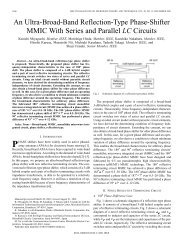
N. Mandolesi et al.: The <strong>Planck</strong>-LFI programmeThe latter are also known as generalized least squares (GLS)methods and are accurate and flexible. Their drawback is that,at the size of the <strong>Planck</strong> data set, they require a significantamount of massively powered computational resources(Poutanen et al. 2006; Ashdown et al. 2007, 2009) andarethusinfeasible to use within a Monte Carlo context. To overcomethe limitations of GLS algorithms, the LFI community has developedso-called “hybrid” algorithms (Keihänen et al. 2005;Kurki-Suonio et al. 2009; Keihänen et al. 2010). These algorithmsrely on a tunable parameter connected to the 1/ f kneefrequency, a measure of the amount of low frequency correlatednoise in the time-ordered data: the higher the knee frequency,the shorter the “baseline” length needed to be chosen toproperly suppress the 1/ f contribution. From this point of view,the GLS solution can be thought of as the limiting case whenthe baseline length approaches the sampling interval. Providedthat the knee frequency is not too high, hybrid algorithms canachieve GLS accuracy at a fraction of the computational demand.Furthermore, they can be tuned to the desired precisionwhen speed is an issue (e.g., for timeline-to-map Monte Carloproduction). The baseline map-making algorithms for LFI is ahybrid code dubbed MADAM.Map-making algorithms can, in general, compute the correlation(inverse covariance) matrix of the map estimate that theyproduce (Keskitalo et al. 2010). At high resolution this computation,though feasible, is impractical, because the size of thematrix makes its handling and inversion prohibitively difficult.At low resolution, the covariance matrix will be produced instead:this is of extreme importance for the accurate characterizationof the low multipoles of the CMB (Keskitalo et al. 2010;Gruppuso et al. 2009).Akeytierof<strong>Planck</strong> data analysis is the separation of astrophysicalfrom cosmological components. A variety of methodshave been developed to this end (e.g., Leach et al. 2008).Point source extraction is achieved by exploiting non-<strong>Planck</strong> catalogues,as well as filtering <strong>Planck</strong> maps with optimal functions(wavelets) capable of recognizing beam-like patterns. In additionto linearly combining the maps or fitting for known templates,diffuse emissions are separated by using the statistical distributionsof the different components, assuming independence betweenthem, or by means of a suitable parametrization and fittingof foreground unknowns on the basis of spatial correlationsin the data or, in alternative, multi-frequency single resolutionelements only.The extraction of statistical information from the CMBusually proceeds by means of correlation functions. Since theCMB field is Gaussian to a large extent (e.g. Smith et al. 2009),most of the information is encoded in the two-point functionor equivalently in its reciprocal representation in spherical harmonicsspace. Assuming rotational invariance, the latter quantityis well described by the set of C l (see e.g., Gorski 1994).For an ideal experiment, the estimated power spectrum could bedirectly compared to a Boltzmann code prediction to constrainthe cosmological parameters. However, in the case of incompletesky coverage (which induces couplings among multipoles)and the presence of noise (which, in general, is not rotationallyinvariant because of the coupling between correlated noise andscanning strategy), a more thorough analysis is necessary. Thelikelihood function for a Gaussian CMB sky can be easily writtenand provides a sound mechanism for constraining modelsand data. The direct evaluation of this function, however, posesintractable computational issues. Fortunately, only the lowestmultipoles require exact treatment. This can be achieved eitherby direct evaluation in the pixel domain or sampling theposterior distribution of the CMB using sampling methods suchas the Gibbs approach (Jewell et al. 2004; Wandelt et al. 2004).At high multipoles, where the likelihood function cannot be evaluatedexactly, a wide range of effective, computationally affordableapproximations exist (see e.g., Hamimeche & Lewis 2008;and Rocha et al., in prep., and references therein). The low andhigh l approaches to power spectrum estimation will be joinedinto a hybrid procedure, pioneered by Efstathiou (2004).The data analysis of LFI will require daunting computationalresources. In view of the size and complexity of its data set, accuratecharacterization of the scientific results and error propagationwill be achieved by means of a massive use of Monte Carlosimulations. A number of worldwide distributed supercomputercentres will support the DPC in this activity. A partial list includesNERSC-LBNL in the USA, CINECA in Italy, CSC inFinland, and MARE NOSTRUM in Spain. The European centreswill benefit from the Distributed European Infrastructure forSupercomputer Application 7 .3. Instrument3.1. OpticsDuring the design phase of LFI, great effort was dedicated to theoptical design of the focal plane unit(FPU).Asalreadymentionedin the introduction, the actual design of the <strong>Planck</strong> telescopeis derived from COBRAS and specially has been tunedby subsequent studies of the LFI team (Villa et al. 1998) andThales-Alenia Space. These studies demonstrated the importanceof increasing the telescope diameter (Mandolesi et al.2000), optimizing the optical design, and also showed how complexit would be to match the real focal surface to the horn phasecentres (Valenziano et al. 1998). The optical design of LFI isthe result of a long iteration process in which the optimizationof the position and orientation of each feed horn involves atrade-off between angular resolution and sidelobe rejection levels(Sandri et al. 2004; Burigana et al. 2004; Sandri et al. 2010).Tight limits were also imposed by means of mechanical constraints.The 70 GHz system has been improved in terms of thesingle horn design and its relative location in the focal surface.As a result, the angular resolution has been maximized.The feed horn development programme started in the earlystages of the mission with prototype demonstrators (Bersanelliet al. 1998), followed by the elegant bread board (Villa et al.2002) andfinallybythequalification(D’Arcangelo et al. 2005)and flight models (Villa et al. 2009). The horn design has a corrugatedshape with a dual profile (Gentili et al. 2000). This choicewas justified by the complexity of the optical interfaces (couplingwith the telescope and focal plane horn accommodation)and the need to respect the interfaces with HFI.Each of the corrugated horns feeds an orthomode transducer(OMT) that splits the incoming signalintotwo orthogonal polarisedcomponents (D’Arcangelo et al. 2009a). The polarisationcapabilities of the LFI are guaranteed by the use of OMTsplaced immediately after the corrugated horns. While the incomingpolarisation state is preserved inside the horn, the OMT dividesit into two linear orthogonal polarisations, allowing LFIto measure the linear polarisation component of the incomingsky signal. The typical value of OMT cross-polarisation isabout −30 dB, setting the spurious polarisation of the LFI opticalinterfaces at a level of 0.001.7 http://www.deisa.euPage 9 of 24
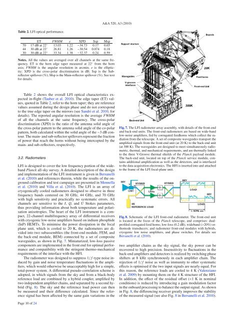
A&A 520, A3 (2010)Table 2. LFI optical performance.ET FWHM e XPD Ssp Msp70 17 dB at 22 ◦ 13.03 1.22 −34.73 0.17 0.6544 30 dB at 22 ◦ 26.81 1.26 −30.54 0.074 0.1830 30 dB at 22 ◦ 33.34 1.38 −32.37 0.24 0.59Notes. All the values are averaged over all channels at the same frequency.ET is the horn edge taper measured at 22 ◦ from the hornaxis; FWHM is the angular resolution in arcmin; e is the ellipticity;XPD is the cross-polar discrimination in dB; Ssp is the Subreflectorspillover (%); Msp is the Main-reflector spillover (%). See textfor details.Table 2 shows the overall LFI optical characteristics expectedin-flight (Tauber et al. 2010). The edge taper (ET) values,quoted in Table 2,refertothehorntaper;theyarereferencevalues assumed during the design phase and do not correspondto the true edge taper on the mirrors (see Sandri et al. 2010, fordetails). The reported angular resolution is the average FWHMof all the channels at the same frequency. The cross-polardiscrimination (XPD) is the ratio of the antenna solid angle ofthe cross-polar pattern to the antenna solid angle of the co-polarpattern, both calculated within the solid angle of the −3dBcontour.The main- and sub-reflector spillovers represent the fractionof power that reach the horns without being intercepted by themain- and sub-reflectors, respectively.3.2. RadiometersLFI is designed to cover the low frequency portion of the wideband<strong>Planck</strong> all-sky survey. A detailed description of the designand implementation of the LFI instrument is given in Bersanelliet al. (2010) andreferencestherein,whiletheresultsoftheongroundcalibration and test campaign are presented in Mennellaet al. (2010) andVilla et al. (2010). The LFI is an array ofcryogenically cooled radiometers designed to observe in threefrequency bands centered on 30 GHz, 44 GHz, and 70 GHzwith high sensitivity and practically no systematic errors. Allchannels are sensitive to the I, Q, andU Stokes parameters,thus providing information about both temperature and polarisationanisotropies. The heart of the LFI instrument is a compact,22-channel multifrequency array of differential receiverswith cryogenic low-noise amplifiers based on indium phosphide(InP) HEMTs. To minimise the power dissipation in the focalplane unit, which is cooled to 20 K, the radiometers are dividedinto two subassemblies (the front-end module, FEM, andthe back-end module, BEM) connected by a set of compositewaveguides, as shown in Fig. 7. Miniaturized,low-losspassivecomponents are implemented in the front end for optimal performanceand compatibility with the stringent thermo-mechanicalrequirements of the interface with the HFI.The radiometer was designed to suppress 1/ f -type noise inducedby gain and noise temperature fluctuations in the amplifiers,which would otherwise be unacceptably high for a simple,total-power system. A differential pseudo-correlation scheme isadopted, in which signals from the sky and from a black-bodyreference load are combined by a hybrid coupler, amplified bytwo independent amplifier chains, and separated by a second hybrid(Fig. 8). The sky and the reference load power can thenbe measured and their difference calculated. Since the referencesignal has been affected by the same gain variations in theFig. 7. The LFI radiometer array assembly, with details of the front-endand back-end units. The front-end radiometers are based on wide-bandlow-noise amplifiers, fed by corrugated feedhorns which collect the radiationfrom the telescope. A set of composite waveguides transport theamplified signals from the front-end unit (at 20 K) to the back-end unit(at 300 K). The waveguides are designed to meet simultaneously radiometric,thermal, and mechanical requirements, and are thermally linkedto the three V-Groove thermal shields of the <strong>Planck</strong> payload module.The back-end unit, located on top of the <strong>Planck</strong> service module, containsadditional amplification as well as the detectors, and is interfacedto the data acquisition electronics. The HFI is inserted into and attachedto the frame of the LFI focal-plane unit.Fig. 8. Schematic of the LFI front-end radiometer. The front-end unitis located at the focus of the <strong>Planck</strong> telescope, and comprises: dualprofiledcorrugated feed horns; low-loss (0.2dB),wideband(>20%) orthomodetransducers; and radiometer front-end modules with hybrids,cryogenic low noise amplifiers, and phase switches. For details seeBersanelli et al. (2010).two amplifier chains as the sky signal, the sky power can berecovered to high precision. Insensitivity to fluctuations in theback-end amplifiers and detectors is realized by switching phaseshifters at 8 kHz synchronously in each amplifier chain. Therejection of 1/ f noise as well as immunity to other systematiceffects is optimised if the two input signals are nearly equal. Forthis reason, the reference loads are cooled to 4 K (Valenzianoet al. 2009) bymountingthemonthe4KstructureoftheHFI.In addition, the effect of the residual offset (
- Page 1 and 2:
A&A 520, E1 (2010)DOI: 10.1051/0004
- Page 3 and 4: ABSTRACTThe European Space Agency
- Page 5 and 6: A&A 520, A1 (2010)Fig. 2. An artist
- Page 7 and 8: A&A 520, A1 (2010)Fig. 4. Planck fo
- Page 9 and 10: A&A 520, A1 (2010)Fig. 6. The Planc
- Page 11 and 12: A&A 520, A1 (2010)Table 4. Summary
- Page 13 and 14: A&A 520, A1 (2010)three frequency c
- Page 15 and 16: A&A 520, A1 (2010)Fig. 12. The left
- Page 17 and 18: A&A 520, A1 (2010)Fig. 14. Left pan
- Page 19 and 20: A&A 520, A1 (2010)flux limit of the
- Page 21 and 22: A&A 520, A1 (2010)- University of C
- Page 23 and 24: A&A 520, A1 (2010)57 Instituto de A
- Page 25 and 26: A&A 520, A2 (2010)Fig. 1. (Left) Th
- Page 27 and 28: A&A 520, A2 (2010)Fig. 3. (Top)Twos
- Page 29 and 30: A&A 520, A2 (2010)Table 2. Predicte
- Page 31 and 32: Table 3. Predicted in-flight main b
- Page 33 and 34: A&A 520, A2 (2010)materials. Theref
- Page 35 and 36: A&A 520, A2 (2010)Fig. 11. Comparis
- Page 37 and 38: A&A 520, A2 (2010)Table 5. Inputs u
- Page 39 and 40: A&A 520, A2 (2010)Fig. 16. Three cu
- Page 41 and 42: A&A 520, A2 (2010)Table 7. Optical
- Page 43 and 44: A&A 520, A2 (2010)Fig. A.1. Dimensi
- Page 45 and 46: A&A 520, A2 (2010)5 Università deg
- Page 47 and 48: A&A 520, A3 (2010)Horizon 2000 medi
- Page 49 and 50: A&A 520, A3 (2010)Fig. 1. CMB tempe
- Page 51 and 52: A&A 520, A3 (2010)Ω ch 2τn s0.130
- Page 53: A&A 520, A3 (2010)Fig. 6. Integral
- Page 57 and 58: 3.3.1. SpecificationsThe main requi
- Page 59 and 60: A&A 520, A3 (2010)Fig. 11. Schemati
- Page 61 and 62: A&A 520, A3 (2010)features of the r
- Page 63 and 64: A&A 520, A3 (2010)Fig. 13. Level 2
- Page 65 and 66: A&A 520, A3 (2010)Fig. 15. Level 3
- Page 67 and 68: A&A 520, A3 (2010)GUI = graphical u
- Page 69 and 70: A&A 520, A3 (2010)23 Centre of Math
- Page 71 and 72: A&A 520, A4 (2010)In addition, all
- Page 73 and 74: A&A 520, A4 (2010)Table 2. Sensitiv
- Page 75 and 76: A&A 520, A4 (2010)Fig. 2. Schematic
- Page 77 and 78: A&A 520, A4 (2010)Fig. 6. LFI recei
- Page 79 and 80: A&A 520, A4 (2010)Fig. 9. Schematic
- Page 81 and 82: A&A 520, A4 (2010)Table 4. Specific
- Page 83 and 84: A&A 520, A4 (2010)Fig. 15. DAE bias
- Page 85 and 86: A&A 520, A4 (2010)Fig. 19. Picture
- Page 87 and 88: A&A 520, A4 (2010)Table 10. Main ch
- Page 89 and 90: Table 13. Principal requirements an
- Page 91 and 92: A&A 520, A5 (2010)DOI: 10.1051/0004
- Page 93 and 94: A. Mennella et al.: LFI calibration
- Page 95 and 96: A. Mennella et al.: LFI calibration
- Page 97 and 98: A. Mennella et al.: LFI calibration
- Page 99 and 100: A. Mennella et al.: LFI calibration
- Page 101 and 102: A. Mennella et al.: LFI calibration
- Page 103 and 104: A. Mennella et al.: LFI calibration
- Page 105 and 106:
D.1. Step 1-extrapolate uncalibrate
- Page 107 and 108:
A&A 520, A6 (2010)DOI: 10.1051/0004
- Page 109 and 110:
F. Villa et al.: Calibration of LFI
- Page 111 and 112:
F. Villa et al.: Calibration of LFI
- Page 113 and 114:
F. Villa et al.: Calibration of LFI
- Page 115 and 116:
F. Villa et al.: Calibration of LFI
- Page 117 and 118:
F. Villa et al.: Calibration of LFI
- Page 119 and 120:
F. Villa et al.: Calibration of LFI
- Page 121 and 122:
A&A 520, A7 (2010)DOI: 10.1051/0004
- Page 123 and 124:
M. Sandri et al.: Planck pre-launch
- Page 126 and 127:
A&A 520, A7 (2010)Fig. 8. Footprint
- Page 128 and 129:
-30-40-30-6-3-20A&A 520, A7 (2010)0
- Page 130 and 131:
A&A 520, A7 (2010)Table 4. Galactic
- Page 132 and 133:
A&A 520, A7 (2010)Fig. A.1. Polariz
- Page 134 and 135:
A&A 520, A8 (2010)inflation, giving
- Page 136 and 137:
A&A 520, A8 (2010)estimated from th
- Page 138 and 139:
A&A 520, A8 (2010)ways the most str
- Page 140 and 141:
unmodelled long-timescale thermally
- Page 142 and 143:
A&A 520, A8 (2010)Fig. 5. Polarisat
- Page 144 and 145:
A&A 520, A8 (2010)Table 3. Band-ave
- Page 146 and 147:
A&A 520, A8 (2010)where S stands fo
- Page 148 and 149:
A&A 520, A8 (2010)Fig. 11. Simulate
- Page 150 and 151:
stored in the LFI instrument model,
- Page 152 and 153:
A&A 520, A8 (2010)Table 5. Statisti
- Page 154 and 155:
A&A 520, A8 (2010)comparable in siz
- Page 156 and 157:
A&A 520, A8 (2010)Table B.1. Main b
- Page 158 and 159:
A&A 520, A8 (2010)Bond, J. R., Jaff
- Page 160 and 161:
A&A 520, A9 (2010)- (v) an optical
- Page 162 and 163:
A&A 520, A9 (2010)Fig. 2. The Russi
- Page 164 and 165:
A&A 520, A9 (2010)Table 3. Estimate
- Page 166 and 167:
A&A 520, A9 (2010)Fig. 7. Picture o
- Page 168 and 169:
A&A 520, A9 (2010)Fig. 9. Cosmic ra
- Page 170 and 171:
A&A 520, A9 (2010)Fig. 13. Principl
- Page 172 and 173:
A&A 520, A9 (2010)Fig. 16. Noise sp
- Page 174 and 175:
A&A 520, A9 (2010)Table 6. Basic ch
- Page 176 and 177:
A&A 520, A9 (2010)with warm preampl
- Page 178 and 179:
A&A 520, A9 (2010)20 Laboratoire de
- Page 180 and 181:
A&A 520, A10 (2010)Table 1. HFI des
- Page 182 and 183:
A&A 520, A10 (2010)based on the the
- Page 184 and 185:
A&A 520, A10 (2010)Fig. 6. The Satu
- Page 186 and 187:
A&A 520, A10 (2010)5. Calibration a
- Page 188 and 189:
A&A 520, A10 (2010)Fig. 16. Couplin
- Page 190 and 191:
A&A 520, A10 (2010)217-5a channel:
- Page 192 and 193:
A&A 520, A10 (2010)10 -310 -495-The
- Page 194 and 195:
A&A 520, A11 (2010)DOI: 10.1051/000
- Page 196 and 197:
P. A. R. Ade et al.: Planck pre-lau
- Page 198 and 199:
P. A. R. Ade et al.: Planck pre-lau
- Page 200 and 201:
P. A. R. Ade et al.: Planck pre-lau
- Page 202 and 203:
A&A 520, A12 (2010)Table 1. Summary
- Page 204 and 205:
arrangement was also constrained by
- Page 206 and 207:
A&A 520, A12 (2010)frequency cut-of
- Page 208 and 209:
A&A 520, A12 (2010)Fig. 9. Gaussian
- Page 210 and 211:
A&A 520, A12 (2010)the horn-to-horn
- Page 212 and 213:
A&A 520, A12 (2010)Fig. 15. Composi
- Page 214 and 215:
A&A 520, A12 (2010)Fig. 19. Broad-b
- Page 216 and 217:
A&A 520, A13 (2010)DOI: 10.1051/000
- Page 218 and 219:
C. Rosset et al.: Planck-HFI: polar
- Page 220 and 221:
C. Rosset et al.: Planck-HFI: polar
- Page 222 and 223:
of frequencies and shown to have po
- Page 224 and 225:
C. Rosset et al.: Planck-HFI: polar
- Page 226 and 227:
C. Rosset et al.: Planck-HFI: polar