N. Mandolesi et al.: The <strong>Planck</strong>-LFI programmeFig. 3. CMB E polarisation modes (black long dashes) compatible withWMAP data and CMB B polarisation modes (black solid lines) for differenttensor-to-scalar ratios of primordial perturbations (r ≡ T/S =1, 0.3, 0.1, at increasing thickness) are compared to WMAP (Ka band,9yearsofobservations)andLFI(30GHz,4surveys)sensitivitytothepower spectrum, assuming the noise expectation has been subtracted.The plots include cosmic and sampling variance plus instrumental noise(green dots for B modes, green long dashes for E modes, labeled withcv+sv+n; black thick dots, noise only) assuming a multipole binning of30% (see caption of Fig. 1 for the meaning of binning and of the numberof sky surveys). Note that the cosmic and sampling (74% sky coverage;as in WMAP polarization analysis, we exclude the sky regions mostlyaffected by Galactic emission) variance implies a dependence of theoverall sensitivity at low multipoles on r (again the green lines refer tor = 1, 0.3, 0.1, from top to bottom), which is relevant to the parameterestimation; instrumental noise only determines the capability of detectingthe B mode. The B mode induced by lensing (blue dots) is alsoshown for comparison.to model more accurately the polarised synchrotron emission,which needs to be removed to greater than the few percent levelto detect primordial B modes for r < ∼ 0.1 (Efstathiou & Gratton2009).2.1.2. Cosmological parametersGiven the improvement relative to WMAP C l achievable withthe higher sensitivity and resolution of <strong>Planck</strong> (as discussed inthe previous section for LFI), correspondingly superior determinationof cosmological parameters is expected. Of course, thebetter sensitivity and angular resolution of HFI channels comparedto WMAP and LFI ones will highly contribute to the improvementin cosmological parameters measured using <strong>Planck</strong>.We present here the comparison between determinations of asuitable set of cosmological parameters using data from WMAP,<strong>Planck</strong>,and<strong>Planck</strong>-LFI alone.In Fig. 5 we compare the forecasts for 1σ and 2σ contoursfor 4 cosmological parameters of the WMAP5 bestfitΛCDM cosmological model: the baryon density; the colddark matter (CDM) density; reionization, parametrized by theThomson optical depth τ; andtheslopeoftheinitialpowerspectrum. These results show the expectation for the <strong>Planck</strong>LFI 70 GHz channel alone after 14 months of observations (redlines), the <strong>Planck</strong> combined 70 GHz, 100 GHz, and 143 GHzchannels for the same integration time (blue lines), and theWMAP five year observations (black lines). We assumed thatthe 70 GHz channels and the 100 GHz and 143 GHz arethe representative channels for LFI and HFI (we note that forFig. 4. As in Fig. 3 but for the sensitivity of WMAP in V band and LFIat 70 GHz, and including also the comparison with Galactic and extragalacticpolarised foregrounds. Galactic synchrotron (purple dashes)and dust (purple dot-dashes) polarised emissions produce the overallGalactic foreground (purple three dot-dashes). WMAP 3-yr power-lawfits for uncorrelated dust and synchrotron have been used. For comparison,WMAP 3-yr results derived directly from the foreground mapsusing the HEALPix package (Górski et al. 2005) areshownoverasuitablemultipole range: power-law fits provide (generous) upper limits tothe power at low multipoles. Residual contamination levels by Galacticforegrounds (purple three dot-dashes) are shown for 10%, 5%, and 3%of the map level, at increasing thickness. The residual contribution ofunsubtracted extragalactic sources, C res,PSl,andthecorrespondinguncertainty,δC res,PSl,arealsoplottedasthickandthingreendashes.Thesearecomputed assuming a relative uncertainty δΠ/Π =δS lim /S lim = 10%in the knowledge of their degree of polarisation and the determinationof the source detection threshold. We assumed the same sky coverageas in Fig. 3. Clearly,foregroundcontaminationislowerat70GHzthanat 30 GHz, but, since CMB maps will be produced from a componentseparation layer (see Sects. 2.3 and 6.3) we considered the same skyregion.HFI we have used angular resolution and sensitivities as givenin Table 1.3 of the <strong>Planck</strong> scientific programme prepared byThe <strong>Planck</strong> Collaboration 2006), for cosmological purposes, respectively,and we assumed a coverage of ∼70% of the sky.Figure 5 shows that HFI 100 GHz and 143 GHz channels arecrucial for obtaining the most accurate cosmological parameterdetermination.While we have not explicitly considered the other channelsof LFI (30 GHz and 44 GHz) and HFI (at frequencies ≥217 GHz)we note that they are essential for achieving the accurate separationof the CMB from astrophysical emissions, particularly forpolarisation.The improvement in cosmological parameter precision forLFI (2 surveys) compared to WMAP5 (Dunkley et al. 2009;Komatsu et al. 2009) isclearfromFig.5. Thisismaximizedfor the dark matter abundance Ω c because of the performance ofthe LFI 70 GHz channel with respect to WMAP5. From Fig. 5 itis clear that the expected improvement for <strong>Planck</strong> in cosmologicalparameter determination compared to that of WMAP5 canopen a new phase in our understanding of cosmology.2.1.3. Primordial non-GaussianitySimple cosmological models assume Gaussian statistics for theanisotropies. However, important information may come frommild deviations from Gaussianity (see e.g., Bartolo et al. 2004,Page 5 of 24
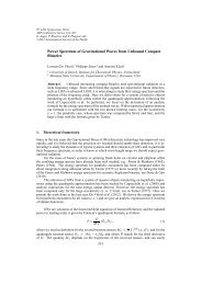
A&A 520, A3 (2010)Ω ch 2τn s0.130.120.110.10.090.150.10.0510.980.960.940.920.022 0.0240.022 0.0240.022 0.0240.150.10.0510.980.960.940.920.022Ω bh 2 0.0240.1 0.120.1 0.120.1 0.12Ω ch 210.980.960.940.05 0.1 0.150.920.05 0.1 0.15τ0.92 0.96 1n sFig. 5. Forecasts of 1σ and 2σ contours for the cosmological parametersof the WMAP5 best-fit ΛCDM cosmological model with reionization,as expected from <strong>Planck</strong> (blue lines) and from LFI alone (red lines)after 14 months of observations. The black contours are those obtainedfrom WMAP five year observations. See the text for more details.for a review). <strong>Planck</strong> total intensity and polarisation data will eitherprovide the first true measurement of non-Gaussianity (NG)in the primordial curvature perturbations, or tighten the existingconstraints (based on WMAP data, see footnote 3) by almost anorder of magnitude.Probing primordial NG is another activity that requires foregroundcleaned maps. Hence, the full frequency maps of bothinstruments must be used for this purpose.It is very important that the primordial NG is model dependent.Asaconsequenceoftheassumedflatnessoftheinflatonpotential, any intrinsic NG generated during standard singlefieldslow-roll inflation is generally small, hence adiabatic perturbationsoriginated by quantum fluctuations of the inflatonfield during standard inflation are nearly Gaussian distributed.Despite the simplicity of the inflationary paradigm, however, themechanism by which perturbations are generated has not yetbeen fully established and various alternatives to the standardscenario have been considered. Non-standard scenarios for thegeneration of primordial perturbations in single-field or multifieldinflation indeed permit higher NG levels. Alternative scenariosfor the generation of the cosmological perturbations, suchas the so-called curvaton, the inhomogeneous reheating, andDBI scenarios (Alishahiha et al. 2004), are characterized by atypically high NG level. For this reason, detecting or even justconstraining primordial NG signals in the CMB is one of themost promising ways to shed light on the physics of the earlyUniverse.The standard way to parameterize primordial non-Gaussianity involves the parameter f NL , which is typicallysmall. A positive detection of f NL ∼ 10 would imply that allstandard single-field slow-roll models of inflation are ruledout. In contrast, an improvement to the limits on the amplitudeof f NL will allow one to strongly reduce the class of nonstandardinflationary models allowed by the data, thus providingunique insight into the fluctuation generation mechanism. Atthe same time, <strong>Planck</strong> temperature and polarisation data willallow different predictions of the shape of non-Gaussianitiesto be tested beyond the simple f NL parameterization. Forsimple, quadratic non-Gaussianity of constant f NL ,theangularbispectrum is dominated by “squeezed” triangle configurationswith l 1 ≪ l 2 ,l 3 .This“local”NGistypicalofmodelsthatproduce the perturbations immediately after inflation (such asfor the curvaton or the inhomogeneous reheating scenarios).So-called DBI inflation models, based on non-canonical kineticterms for the inflaton,leadtonon-localformsofNG,whicharedominated by equilateral triangle configurations. It has beenpointed out (Holman & Tolley 2008) that excited initial states ofthe inflaton may lead to a third shape, called “flattened” triangleconfiguration.The strongest available CMB limits on f NL for local NGcomes from WMAP5. In particular, Smith et al. (2009)obtained−4 < f NL < 80 at 95% confidence level (C.L.) using the optimalestimator of local NG. <strong>Planck</strong> total intensity and polarisationdata will allow the window on | f NL | to be reduced below ∼10.Babich & Zaldarriaga (2004) andYadav et al. (2007) demonstratedthat a sensitivity to local non-Gaussianity ∆ f NL ≈ 4(at 1σ) is achievable with <strong>Planck</strong>. Wenotethataccuratemeasurementof E-type polarisation will play a significant role inthis constraint. Note also that the limits that <strong>Planck</strong> can achievein this case are very close to those of an “ideal” experiment.Equilateral-shape NG is less strongly constrained at present,with −125 < f NL < 435 at 95% C.L. (Senatore et al. 2010).In this case, <strong>Planck</strong> will also have a strong impact on this constraint.Various authors (Bartolo & Riotto 2009)haveestimatedthat <strong>Planck</strong> data will allow us to reduce the bound on | f NL | toaround 70.Measuring the primordial non-Gaussianity in CMB data tothese levels of precision requires accurate handling of possiblecontaminants, such as those introduced by instrumental noiseand systematics, by the use of masks and imperfect foregroundand point source removal.2.1.4. Large-scale anomaliesObservations of CMB anisotropies contributed significantly tothe development of the standard cosmological model, alsoknown as the ΛCDM concordance model. This involves a set ofbasic quantities for which CMB observations and other cosmologicaland astrophysical data-sets agree: spatial curvature closeto zero; ≃70% of the cosmic density in the form of dark energy;≃20% in CDM; 4−5% in baryonic matter; and a nearly scaleinvariantadiabatic, Gaussian primordial perturbations. Althoughthe CMB anisotropy pattern obtained by WMAP is largely consistentwith the concordance ΛCDM model, there are some interestingand curious deviations from it, in particular on the largestangular scales. Probing these deviations has required carefulanalysis procedures and so far are at only modest levels of significance.The anomalies can be listed as follows:– Lack of power on large scales. The angular correlation functionis found to be uncorrelated (i.e., consistent with zero)for angles larger than 60 ◦ .InCopi et al. (2007, 2009), it wasshown that this event happens in only 0.03% of realizationsof the concordance model. This is related to the surprisinglylow amplitude of the quadrupole term of the angularpower spectrum already found by COBE (Smoot et al.1992; Hinshaw et al. 1996), and now confirmed by WMAP(Dunkley et al. 2009; Komatsu et al. 2009).Page 6 of 24
- Page 1 and 2: A&A 520, E1 (2010)DOI: 10.1051/0004
- Page 3 and 4: ABSTRACTThe European Space Agency
- Page 5 and 6: A&A 520, A1 (2010)Fig. 2. An artist
- Page 7 and 8: A&A 520, A1 (2010)Fig. 4. Planck fo
- Page 9 and 10: A&A 520, A1 (2010)Fig. 6. The Planc
- Page 11 and 12: A&A 520, A1 (2010)Table 4. Summary
- Page 13 and 14: A&A 520, A1 (2010)three frequency c
- Page 15 and 16: A&A 520, A1 (2010)Fig. 12. The left
- Page 17 and 18: A&A 520, A1 (2010)Fig. 14. Left pan
- Page 19 and 20: A&A 520, A1 (2010)flux limit of the
- Page 21 and 22: A&A 520, A1 (2010)- University of C
- Page 23 and 24: A&A 520, A1 (2010)57 Instituto de A
- Page 25 and 26: A&A 520, A2 (2010)Fig. 1. (Left) Th
- Page 27 and 28: A&A 520, A2 (2010)Fig. 3. (Top)Twos
- Page 29 and 30: A&A 520, A2 (2010)Table 2. Predicte
- Page 31 and 32: Table 3. Predicted in-flight main b
- Page 33 and 34: A&A 520, A2 (2010)materials. Theref
- Page 35 and 36: A&A 520, A2 (2010)Fig. 11. Comparis
- Page 37 and 38: A&A 520, A2 (2010)Table 5. Inputs u
- Page 39 and 40: A&A 520, A2 (2010)Fig. 16. Three cu
- Page 41 and 42: A&A 520, A2 (2010)Table 7. Optical
- Page 43 and 44: A&A 520, A2 (2010)Fig. A.1. Dimensi
- Page 45 and 46: A&A 520, A2 (2010)5 Università deg
- Page 47 and 48: A&A 520, A3 (2010)Horizon 2000 medi
- Page 49: A&A 520, A3 (2010)Fig. 1. CMB tempe
- Page 53 and 54: A&A 520, A3 (2010)Fig. 6. Integral
- Page 55 and 56: A&A 520, A3 (2010)Table 2. LFI opti
- Page 57 and 58: 3.3.1. SpecificationsThe main requi
- Page 59 and 60: A&A 520, A3 (2010)Fig. 11. Schemati
- Page 61 and 62: A&A 520, A3 (2010)features of the r
- Page 63 and 64: A&A 520, A3 (2010)Fig. 13. Level 2
- Page 65 and 66: A&A 520, A3 (2010)Fig. 15. Level 3
- Page 67 and 68: A&A 520, A3 (2010)GUI = graphical u
- Page 69 and 70: A&A 520, A3 (2010)23 Centre of Math
- Page 71 and 72: A&A 520, A4 (2010)In addition, all
- Page 73 and 74: A&A 520, A4 (2010)Table 2. Sensitiv
- Page 75 and 76: A&A 520, A4 (2010)Fig. 2. Schematic
- Page 77 and 78: A&A 520, A4 (2010)Fig. 6. LFI recei
- Page 79 and 80: A&A 520, A4 (2010)Fig. 9. Schematic
- Page 81 and 82: A&A 520, A4 (2010)Table 4. Specific
- Page 83 and 84: A&A 520, A4 (2010)Fig. 15. DAE bias
- Page 85 and 86: A&A 520, A4 (2010)Fig. 19. Picture
- Page 87 and 88: A&A 520, A4 (2010)Table 10. Main ch
- Page 89 and 90: Table 13. Principal requirements an
- Page 91 and 92: A&A 520, A5 (2010)DOI: 10.1051/0004
- Page 93 and 94: A. Mennella et al.: LFI calibration
- Page 95 and 96: A. Mennella et al.: LFI calibration
- Page 97 and 98: A. Mennella et al.: LFI calibration
- Page 99 and 100: A. Mennella et al.: LFI calibration
- Page 101 and 102:
A. Mennella et al.: LFI calibration
- Page 103 and 104:
A. Mennella et al.: LFI calibration
- Page 105 and 106:
D.1. Step 1-extrapolate uncalibrate
- Page 107 and 108:
A&A 520, A6 (2010)DOI: 10.1051/0004
- Page 109 and 110:
F. Villa et al.: Calibration of LFI
- Page 111 and 112:
F. Villa et al.: Calibration of LFI
- Page 113 and 114:
F. Villa et al.: Calibration of LFI
- Page 115 and 116:
F. Villa et al.: Calibration of LFI
- Page 117 and 118:
F. Villa et al.: Calibration of LFI
- Page 119 and 120:
F. Villa et al.: Calibration of LFI
- Page 121 and 122:
A&A 520, A7 (2010)DOI: 10.1051/0004
- Page 123 and 124:
M. Sandri et al.: Planck pre-launch
- Page 126 and 127:
A&A 520, A7 (2010)Fig. 8. Footprint
- Page 128 and 129:
-30-40-30-6-3-20A&A 520, A7 (2010)0
- Page 130 and 131:
A&A 520, A7 (2010)Table 4. Galactic
- Page 132 and 133:
A&A 520, A7 (2010)Fig. A.1. Polariz
- Page 134 and 135:
A&A 520, A8 (2010)inflation, giving
- Page 136 and 137:
A&A 520, A8 (2010)estimated from th
- Page 138 and 139:
A&A 520, A8 (2010)ways the most str
- Page 140 and 141:
unmodelled long-timescale thermally
- Page 142 and 143:
A&A 520, A8 (2010)Fig. 5. Polarisat
- Page 144 and 145:
A&A 520, A8 (2010)Table 3. Band-ave
- Page 146 and 147:
A&A 520, A8 (2010)where S stands fo
- Page 148 and 149:
A&A 520, A8 (2010)Fig. 11. Simulate
- Page 150 and 151:
stored in the LFI instrument model,
- Page 152 and 153:
A&A 520, A8 (2010)Table 5. Statisti
- Page 154 and 155:
A&A 520, A8 (2010)comparable in siz
- Page 156 and 157:
A&A 520, A8 (2010)Table B.1. Main b
- Page 158 and 159:
A&A 520, A8 (2010)Bond, J. R., Jaff
- Page 160 and 161:
A&A 520, A9 (2010)- (v) an optical
- Page 162 and 163:
A&A 520, A9 (2010)Fig. 2. The Russi
- Page 164 and 165:
A&A 520, A9 (2010)Table 3. Estimate
- Page 166 and 167:
A&A 520, A9 (2010)Fig. 7. Picture o
- Page 168 and 169:
A&A 520, A9 (2010)Fig. 9. Cosmic ra
- Page 170 and 171:
A&A 520, A9 (2010)Fig. 13. Principl
- Page 172 and 173:
A&A 520, A9 (2010)Fig. 16. Noise sp
- Page 174 and 175:
A&A 520, A9 (2010)Table 6. Basic ch
- Page 176 and 177:
A&A 520, A9 (2010)with warm preampl
- Page 178 and 179:
A&A 520, A9 (2010)20 Laboratoire de
- Page 180 and 181:
A&A 520, A10 (2010)Table 1. HFI des
- Page 182 and 183:
A&A 520, A10 (2010)based on the the
- Page 184 and 185:
A&A 520, A10 (2010)Fig. 6. The Satu
- Page 186 and 187:
A&A 520, A10 (2010)5. Calibration a
- Page 188 and 189:
A&A 520, A10 (2010)Fig. 16. Couplin
- Page 190 and 191:
A&A 520, A10 (2010)217-5a channel:
- Page 192 and 193:
A&A 520, A10 (2010)10 -310 -495-The
- Page 194 and 195:
A&A 520, A11 (2010)DOI: 10.1051/000
- Page 196 and 197:
P. A. R. Ade et al.: Planck pre-lau
- Page 198 and 199:
P. A. R. Ade et al.: Planck pre-lau
- Page 200 and 201:
P. A. R. Ade et al.: Planck pre-lau
- Page 202 and 203:
A&A 520, A12 (2010)Table 1. Summary
- Page 204 and 205:
arrangement was also constrained by
- Page 206 and 207:
A&A 520, A12 (2010)frequency cut-of
- Page 208 and 209:
A&A 520, A12 (2010)Fig. 9. Gaussian
- Page 210 and 211:
A&A 520, A12 (2010)the horn-to-horn
- Page 212 and 213:
A&A 520, A12 (2010)Fig. 15. Composi
- Page 214 and 215:
A&A 520, A12 (2010)Fig. 19. Broad-b
- Page 216 and 217:
A&A 520, A13 (2010)DOI: 10.1051/000
- Page 218 and 219:
C. Rosset et al.: Planck-HFI: polar
- Page 220 and 221:
C. Rosset et al.: Planck-HFI: polar
- Page 222 and 223:
of frequencies and shown to have po
- Page 224 and 225:
C. Rosset et al.: Planck-HFI: polar
- Page 226 and 227:
C. Rosset et al.: Planck-HFI: polar