Planck Pre-Launch Status Papers - APC - Université Paris Diderot ...

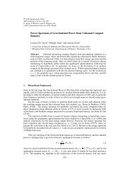
C. Rosset et al.: Planck-HFI: polarization calibration7.2. Orientation ground measurements7.2.1. The calibration setupThe orientation calibration was performed within a 1-m diametercryostat cooled to 2 K, to be close to flight conditions (for a moredetailed description of the calibration setup and photographs, seePajot et al. 2010). The detectors were cooled to their nominaloperating temperature, 100 mK. For polarization measurements,the source (Cold Source 2 or CS2) was a blackbody at 20 Kwhose radiation was diluted within a 50 cm diameter sphere inorder to illuminate, after a reflection from mirror, the full focalplane at once. The source was modulated by a diapason at a fixedfrequency of 10 Hz. The radiation was linearly polarized by analuminum grid deposited on a 138 mm diameter mylar film. Thealuminum strips of the polarizer were 5 µm wide,5µm thickand spaced 5 µm apart.TheMylarfilmitselfwas10µm thick,with a transmission coefficient greater than 0.9; the polarizationefficiency of the polarizer was measured to be better than 99.9%,so it can be assumed equal to unity at HFI frequencies. The polarizercould rotate freely around its axis using a stepper motor.There are exactly 32 000 steps in one rotation, so the precisionin relative angle is better than 1 ′ .7.2.2. Reference for angle measurementThe reference position was defined by a pin fixed to the polarizer,which was detected by electric contact with a copper stripwith a precision of ±5motorsteps,i.e.±0. ◦ 06. We measured theangle of this reference position with respect to the focal planeusing the light of a laser diffracted by the strips of the polarizer;the diffraction pattern is formed by points aligned orthogonallyto the strips (i.e. parallel to the transmitted polarization).Two different methods were used to determine polarizationangles with respect to the focal plane. In the first method, wemeasured the orientation with respect to the platform and usedthe mechanical position of the instrument with respect to theplatform to get the absolute angle. In the second method, wemeasured the angle directly with respect to the instrument. Inboth cases, we measured the same angle and checked it wasconstant across the polarizer. Both methods gave similar errorestimates on the reference position angle, which can safely beassumed to be lower than 0. ◦ 3:∣∣∆θ absolute∣ ∣ < 0. ◦ 3. (41)7.2.3. Data analysisFor this measurement, the polarizer was rotated by 5 ◦ steps andsignal was inegrated for 20 s at each position. Eight full rotationsof the polarizer were performed.At each polarizer position, the signal from the source is sinusoidalwith a frequency of 10 Hz. It is demodulated fitting asine curve over a few periods, yielding around 60 independentmeasurements for each stationary period of 20 s. The averageand standard deviation of these 60 measurements give the signaland its error for each 20 s period, for a fixed position of the polarizer.The statistical error was found to be typically below 1%of the signal.We then fit the signal as a function of the polarizer angleto estimate the polarization efficiency and the orientationof the detectors. However, despite the good quality of the polarizer,we found cross-polarization leakage of around 30%,much higher than that found in Sect. 7.1, withtheCardiff measurements:it was probably due to standing waves between theFig. 9. Signal of PSB 100-1b with respect to the angle in the horn apertureplane; each color represents one rotation of the polarizer (8 turns);the signal is fitted using a standard sine curve. The difference exhibits asystematic effect that can be explained by standing waves between thepolarizer and the focal plane (see text).polarizer and the focal plane and made the detector polarizationefficiency unmeasurable with this setup. The angle that maximizesthe signal gives the orientation of the polarizer; however,the PSB angle must be given in the horn aperture plane, whichis slightly out of parallel with the polarizer plane. We have performedray-tracing simulations to estimate and correct for thisgeometrical effect. The corrections lie between −0. ◦ 5to0. ◦ 5, andthe precision (set by the precision on the position of the polarizer)is better than 0. ◦ 15.Figure 9 shows the curve obtained for a PSB at 100 GHzand the difference with the fitted model. The residuals showa90 ◦ -periodic sine curve, which is present in some detectors.Some detectors also have glitches, reproduced at the same positionat each rotation of the polarizer. These glitches mostlyaffect the highest two frequency channels (545 and 857 GHz),i.e., only SWBs. As cos 2θ and cos 4θ are orthogonal functionsover 2π, thefittedvaluesfortheangleandthepolarizationefficiencyare unchanged when adding such a term in the fittingmodel. However, we cannot exclude that they may be contaminatedby a systematic effect like some other modes (mainly inmode cos 4θ). For example, if the incoming radiation is the sumof two partially linearly polarized radiations, one with orientationθ (rotating with the polarizer) and one with fixed orientationθ 0 ,thesignalmeasuredbythedetectorreads:s(θ) ∝ 1 + ρ cos 2(θ − θ det )+ ρ ′ cos 2(θ − θ 0 )[1− cos 2(θ − θ det )] (42)where θ det is the polarization orientation of the detector. In thismodel, the angle measured through the phase of the mode cos 2θwill not be the detector polarization angle.More generally, we can expand the signal as a Fourier seriess(θ) = ∑ +Nn=−N c n e inθ and fit its coefficients c n (which fulfill thecondition c ⋆ −n = c n,ass is a real quantity). The coefficient c 2 ,giving the dependence in cos 2θ, containstheinformationonpolarization efficiency and angle through its modulus and argument,and is independent of the other modes. To estimate theerror on the polarization angle without relying on a particularmodel, we assume that the mode c 2 is the sum of two contributions,c 2 = c pol2+ c syst2(true polarization signal and inducedPage 9 of 12