Planck Pre-Launch Status Papers - APC - Université Paris Diderot ...

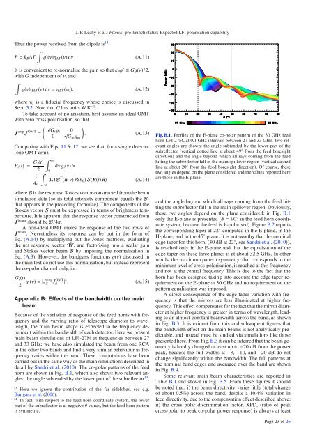
J. P. Leahy et al.: Planck pre-launch status: Expected LFI polarisation capabilityThus the power received from the dipole is 13∫P = k B ∆T g ′ (ν)η ∆T (ν)dν(A.11)It is convenient to re-normalise the gain so that k B g ′ ≡ Gg(ν)/2,with G independent of ν, and∫g(ν)η ∆T (ν)dν = η ∆T (ν 0 ),(A.12)where ν 0 is a fiducial frequency whose choice is discussed inSect. 5.2.NotethatG has units W K −1 .To take account of polarisation, first assume an ideal OMTwith zero cross polarisation, so that( √ )J amp J OMT Gs g= s√0. (A.13)0 Gm g mComparing with Eqs. 11 & 12,weseethat,forasingledetector(one OMT arm),P i (t) = G i(t)2∫14π∫ ∞4π0dνg i (ν) ×dΩ B T ( ˆn,ν) R(θ 0 ) S(R(t) ˆn)(A.14)where B is the response Stokes vector constructed from the beamsimulation data (so its total-intensity component equals the B Ithat appears in the preceding formulae). The components of theStokes vector S must be expressed in terms of brightness temperature.It is apparent that the response vector constructed fromJ beam should be B/4π.Anon-idealOMTmixestheresponseofthetworowsofJ beam . Nevertheless its response can be put in the form ofEq. (A.14) bymultiplyingouttheJonesmatrices,evaluatingthe net response vector W, andfactorisingintoascalargainand Stokes vector beam B by imposing the normalisation inEq. (A.3). However, the bandpass functions g(ν) discussedinthe main text do not use this normalisation, but instead representthe co-polar channel only, i.e.G i (t)2 g i(ν) = |J ampiiJii OMT | 2 . (A.15)Appendix B: Effects of the bandwidth on the mainbeamBecause of the variation of response of the feed horns with frequencyand the varying ratio of telescope diameter to wavelength,the main beam shape is expected to be frequency dependentwithin the bandwidth of each detector. Here we presentmain beam simulations of LFI-27M at frequencies between 27and 33 GHz; we have also simulated the beam from one RCAin the other two bands and find a very similar behaviour as frequencyvaries within the band. These computations have beencarried out in the same way as the main simulations described indetail by Sandri et al. (2010). The co-polar patterns of the feedhorn are shown in Fig. B.1, whichalsoshowstworelevantangles:the angle subtended by the lower part of the subreflector 14 ,13 Here we ignore the contribution of the far sidelobes, see e.g.Burigana et al. (2006).14 In fact, with respect to the feed horn coordinate system, the lowerpart of the subreflector is at negative θ values, but the feed horn patternis symmetric.Fig. B.1. Profiles of the E-plane co-polar pattern of the 30 GHz feedhorn LFI-27M, at 0.1 GHz intervals between 27 and 33 GHz. Two relevantangles are shown: the angle subtended by the lower part of thesubreflector (vertical dotted line at about 49 ◦ from the feed boresightdirection) and the angle beyond which all rays coming from the feedhitting the subreflector fall in the main spillover region (vertical dashedline at about 20 ◦ from the feed boresight direction). Of course, thesetwo angles depend on the plane considered and the values reported hereare those in the E-plane.and the angle beyond which all rays coming from the feed hittingthe subreflector fall in the main spillover region. Obviously,these two angles depend on the plane considered: in Fig. B.1only the E-plane is presented (φ = 90 ◦ in the feed horn coordinatesystem, because the feed is Y-polarised). Figure B.2 reportsthe corresponding taper at 22 ◦ computed in the E-plane, in theH-plane, and in the 45 ◦ plane. It is noteworthy that the nominaledge taper for this horn, (30 dB at 22 ◦ ,seeSandri et al. (2010)),is reached only in the E-plane and that the equalisation of theedge taper on these three planes is at about 32.5 GHz. In otherwords, the maximum pattern symmetry, that corresponds to theminimum level of cross-polarisation, is reached at this frequencyand not at the central frequency. This is due to the fact that thehorn has been designed taking into account the edge taper requirementon the E-plane at 30 GHz and no requirement on thepattern equalisation was imposed.Adirectconsequenceoftheedgetapervariationwithfrequencyis that the mirrors are less illuminated at higher frequency.This effect compensates for the fact that the mirror diameterat higher frequency is greater in terms of wavelength, leadingto an almost-constant beamwidth across the band, as shownin Fig. B.3. Itisevidentfromthisandsubsequentfiguresthatthe bandwidth effect on the main beams is not analytically predictable,and instead must be studied via simulations like thosepresented here. From Fig. B.3 it can be inferred that the beam geometryis hardly changed at least up to −20 dB from the powerpeak, because the full widths at −3, −10, and −20 dB do notchange significantly within the bandwidth. The full patterns atthe nominal band edges and averaged over the band are shownin Fig. B.4.Some relevant main beam characteristics are reported inTable B.1 and shown in Fig. B.5. Fromthesefiguresitshouldbe noted that: i) the beam directivity varies little (total changeof about 0.5%) across the band, despite a 10.4% variation infeed directivity, due to the compensation effect described above;ii) the cross polar discrimination factor, XPD, (ratio of peakcross-polar to peak co-polar power response) is always at leastPage 23 of 26