Planck Pre-Launch Status Papers - APC - Université Paris Diderot ...

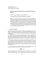
J. P. Leahy et al.: Planck pre-launch status: Expected LFI polarisation capabilityminima are D = 0.21 and 1.07 mK, compared to a median valueof D ≈ D 0 sin 45 ◦ = 2.4mK.Thus,althoughtypicallythedipoleallows calibration to < ∼ 1% in an hour (Sect. 5.1), during the lowestdipole period the calibration precision will be ten times worsethan the median.In addition to the CMB dipole, a strong signal is availableat each crossing of the Galactic plane. Unfortunately this has adifferent spectral shape from the CMB and therefore a different“colour correction” (see Sect. 5.2). Further, we do not haveaccurate prior knowledge of the Galactic brightness at LFI frequencies.Therefore the brightest parts of the Galactic plane willbe masked and the remainder modelled and subtracted when derivinggain factors. Similarly, as noted by Cappellini et al., theCMB fluctuations themselves can be a significant source of error,especially during low-dipole periods, if no correction for themis made. Fortunately, calibration errors are a second-order effect,so the CMB fluctuations and high-latitude foregrounds canbe mapped with sufficient accuracy to correct for their effect oncalibration even before final gain values have been derived.7.5.2. Analysis of simulationsTo assess the impact of random errors in the gain calibration onthe polarisation maps, we re-analysed the “Trieste” simulationsmade by Ashdown et al. (2009). These were simulated observationsby the Planck 30-GHz system, with a fairly realistic scanstrategy in a 1-year survey. In the simulation, the spin axis wasfixed for 1-h “pointing periods” (actual pointing periods will beshorter on average and have variable lengths). At the two periodsof dipole minima, the dipole amplitudes were 0.49 and 0.81 mK,so this is not as asymmetric as the likely flight pattern. The annualdipole was not included but would have made very little differencefor the assumed scan strategy. The model sky comprisedmany components, including polarised Galactic foregrounds, butrealism was not a high priority; in particular, the Galactic planeis much too highly polarised in the light of WMAP results.Simulated timelines for foregrounds, CMB, dipole, and noisewere prepared separately, facilitating our analysis. We re-scaledthe noise to values consistent with those reported by Meinholdet al. (2009), and the calibration procedure was simulated byfitting the dipole+destriped noise to find a gain factor for eachpointing period. We refer to this as case B (case A will follow).This does not include the iterative procedure needed to correctfor CMB fluctuations and foregrounds. Our error estimates areoptimistic, since they do not account for masking of the strongforeground features, in particular the Galactic plane; in generalthis will affect only a small fraction of each scan circle but it happensto have its largest impact when the dipole signal is weakest,as we see below. Figure 15 shows an example run of estimatedgain differences: the increased scatter in March and Septemberis obvious.We also simulated the impact of ignoring the CMB fluctuationsby fitting the CMB + dipole + noise to a dipole (case A).As expected the residual errors were much larger (σ γ = 1.2%vs. 0.3% per hour over the full year), but also as expected, theyare highly correlated between the main and side arms, since theCMB fluctuations are predominantly unpolarised; in fact plotssuch as Fig. 15 for the two cases are virtually indistinguishable.This is the term that controls polconversion (Eq. (9)), and evidentlyit is highly insensitive to errors in modelling the nondipoleemission.The data for each polarisation of each detector were multipliedby the appropriate gain factor to simulate random calibrationerrors, and the Ĩ and ˜Q H signal streams were used to(γs − γm)/20.0150.010.0050−0.005−0.01−0.015RMS = 0.001915RMS = 0.0003741000 2000 3000 4000 5000 6000 7000 8000Time [hour]Fig. 15. Gain error difference (γ s − γ m )/2 betweensideandmainarmradiometers of the LFI-27 horn. The plot is for a 1 year survey. Redline: gains were obtained by fitting the dipole signal to each 1-h pointingperiod. Black line: 6-day binning of the 1-h gains. The RMS values givethe standard deviation of 1-h and 6-day gain error differences.create maps of (I, Q, U), using the MADAM destriping mapmaker(Keihänen et al. 2005; Keihänen et al. 2010), as in theoriginal analysis by Ashdown et al. (2009). We also producedand mapped a second set of timelines where the calibration factorshad been averaged for 6 days by simple binning. SinceMADAM is a linear process it is meaningful to analyse signal-onlymaps to isolate the errors due to miscalibration. Figure 16 showsthe difference between the signal-only maps with and withoutthe residual gain errors, for Stokes I and Q.As expected for a multiplicative effect, the largest residualsare along the Galactic plane. At high Galactic latitudes thesystematic variation of gain precision is not apparent, becausethe residuals are proportional to γI, whereI is the local skysignal and is dominated by the dipole. Since γ, thefractionalcalibration error, is inversely proportional to the dipole signalon the scan circle, the rms value of γI does not vary systematicallywith ecliptic longitude; instead a strong ecliptic latitudeeffect is seen due to the increasing density of scan crossings inthe deep regions near the poles, mirroring the pattern for whitenoise. At low Galactic latitude the situation is different becausethe strong Galactic signal is not used for the calibration. The relativelylarge gain errors during the two low-dipole periods giverise to large residuals along the corresponding scan circles, nearecliptic longitudes 90 ◦ from the dipole direction, which cross theplane at Galactic longitudes of 170 ◦ and 350 ◦ ,andalsocrossthebright Orion complex near the anticentre. These scans cross theplane at a relatively small angle, so masking the plane will affecta significant fraction of the scan length, further degradingthe calibration; this awkward geometry is fixed by the relativeorientation of the dipole and the Galaxy.The amplitudes of the residuals for I and Q are rather similar,since the Q residuals are mainly due to polconversion from Iand not to distortion of the true Q signal. The magnitude of theon-sky residuals is significantly smaller than the naive estimateof |γI|, becauseeachpixelcontainscontributions from severalindependent pointing periods and detectors.While ideally we would have run a Monte-Carlo seriesto characterise these errors, a single realisation gives aPage 19 of 26