Planck Pre-Launch Status Papers - APC - Université Paris Diderot ...

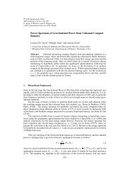
unmodelled long-timescale thermally-driven gain changes willof course be calibrated along with the stochastic 1/ f component.At present there are no test data runs longer than a few hoursfor the LFI radiometers in which they operated at nominal conditions,so the outer cutoff for LFI will be established during theon-orbit calibration phase.Astronomical gain calibration is based on the CMB dipole,which appears as a fluctuation at the satellite spin frequency inthe time-ordered data, with Rayleigh-Jeans amplitude η ∆T (ν 0 )D;this varies through the year due to geometric effects, as discussedin Sect. 7.5. Iferrorsaredominatedbynoise,the1-σ error in γisσ(γ) =σ T√2τη∆T (ν 0 )D√1 +(fspinf knee) α(23)for an integration time τ and a 1-second white noise level of σ T .The last term allows for the effect of 1/ f noise (Meinhold et al.2009). For reference, taking the median value, D = 2.4 mK,and noise parameters from Meinhold et al. (2009), we get σ γ =0.56%, 0.41%, and 0.24% at 70, 44, and 30 GHz, respectivelyfor a 1-h integration. The impact of residual gain errors on themaps is discussed in Sect. 7.5.A&A 520, A8 (2010)5.2. Bandpass differencesOur formalism for describing the effect of finite bandwidthson differencing polarimetry was briefly described by Leahy &Foley (2006); a more detailed presentation is in preparation. Themost basic effect is to render ambiguous the operating frequencyquoted for a detector: it is helpful to distinguish the nominal frequencyused to label the band (30, 44 and 70 GHz for the LFI),the fiducial frequency for each band, ν 0 ,chosentominimisethephotometric errors to be described in this section, and the effectivefrequency for each detector, ν eff ,atwhichsucherrorsarezero for a reference spectrum.In an idealised model of gain calibration, a perfect measurementof the power due to the dipole, P dipole ,givesagainestimateof˜G =2P dipoleη ∆T (ν 0 )D = G ∫ ∞g(ν) η0 ∆T (ν)dν= G. (24)η ∆T (ν 0 )The corrected total intensity in Rayleigh-Jeans units for an unpolarisedsource with spectrum I(ν) willthenbeĨ = 2P˜G ∫ ∞= g(ν)I(ν)dν ≡ [ 1 + f (β, ν 0 ) ] I(ν 0 ). (25)0In general β must stand for a vector of parameters controlling thesource spectral shape, but in practice a single spectral index oftensuffices over the 20–30% frequency range of a Planck bandpass.The f factor is a contribution to the band-integrated gainerror γ; itisequivalenttoacolourterminopticalphotometry.For a given source spectrum and bandpass there is an effectivefrequency for which f will be zero (Fig. 4); by construction it isalso automatically zero when the source spectrum is η ∆T ,independentlyof ν 0 .Forthisreasonweconsiderf to be an error thataffects foreground emission only and writeĨ = η ∆T (ν 0 )∆T CMB + [1 + f (β, ν 0 )]I F (ν 0 ), (26)where I F is the foreground brightness. Then β refers to the foregroundemission only; we emphasise that it varies from pixel topixel and band to band.Fig. 4. Plots of effective frequency ν eff against spectral index β, definedby f (β, ν eff ) = 0, for a pure power-law sky spectrum, for each LFI detector.Solid lines are side-arm and dashed main-arm. The glitch nearβ CMB ≈ 0occursbecausespectratrackingtheCMBhavemultiplevaluesof ν eff ,sincebyconstructionthecolourterm f (β CMB ,ν)isnearlyzero for all frequencies.We apply this formalism to the current best estimates of theLFI bandpasses, namely the QUCS models from Zonca et al.(2009). To minimise the error in the total intensity maps, wedefine ν 0 for each LFI band to be the mean of the individualdetector ν eff values, when observing the dominant foregroundPage 8 of 26