Planck Pre-Launch Status Papers - APC - Université Paris Diderot ...

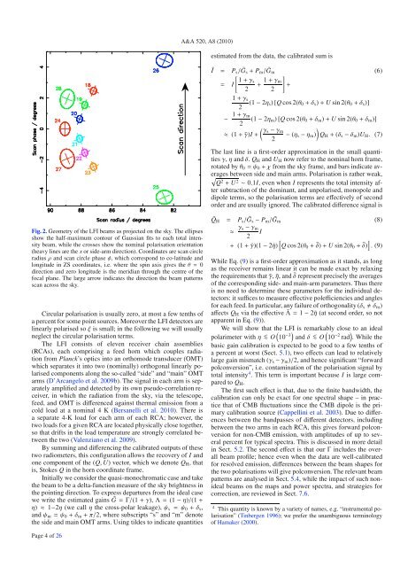
A&A 520, A8 (2010)estimated from the data, the calibrated sum isĨ = P s / ˜G s + P m / ˜G m (6)[ 1 + γs= I + 1 + γ ]m+2 21 + γ s(1 − 2η s )[Q cos 2(θ 0 + δ s ) + U sin 2(θ 0 + δ s )]2− 1 + γ m(1 − 2η m )[Q cos 2(θ 0 + δ m ) + U sin 2(θ 0 + δ m )]2( γs − γ)m≈ (1 + ¯γ)I + − (η s − η m ) Q H + (δ s − δ m )U H . (7)2The last line is a first-order approximation in the small quantitiesγ, η and δ. Q H and U H now refer to the nominal horn frame,rotated by θ 0 = ψ 0 + χ from the sky frame, and bars indicate averagesbetween side and main arms. Polarisation is rather weak,√Q2 + U 2 ∼ 0.1I, evenwhenI represents the total intensity aftersubtraction of the dominant, and unpolarised, monopole anddipole terms, so the polarisation terms are effectively of secondorder and are usually ignored. The calibrated difference signal isFig. 2. Geometry of the LFI beams as projected on the sky. The ellipsesshow the half-maximum contour of Gaussian fits to each total intensitybeam, while the crosses show the nominal polarisation orientation(heavy lines are the x or side-arm direction). Coordinates are scan circleradius ρ and scan circle phase φ, whichcorrespondtoco-latitudeandlongitude in ZS coordinates, i.e. where the spin axis gives the θ = 0direction and zero longitude is the meridian through the centre of thefocal plane. The large arrow indicates the direction the beam patternsscan across the sky.Circular polarisation is usually zero, at most a few tenths ofapercentforsomepointsources.MoreovertheLFIdetectorsarelinearly polarised so ξ is small; in the following we will usuallyneglect the circular polarisation terms.The LFI consists of eleven receiver chain assemblies(RCAs), each comprising a feed horn which couples radiationfrom Planck’s optics into an orthomode transducer (OMT)which separates it into two (nominally) orthogonal linearly polarisedcomponents along the so-called “side” and “main” OMTarms (D’Arcangelo et al. 2009b). The signal in each arm is separatelyamplified and detected by its own pseudo-correlation receiver,in which the radiation from the sky, via the telescope,feed, and OMT is differenced against thermal emission from acold load at a nominal 4 K (Bersanelli et al. 2010). There isaseparate4-KloadforeacharmofeachRCA;however,thetwo loads for a given RCA are located physically close together,so that drifts in the load temperature are strongly correlated betweenthe two (Valenziano et al. 2009).By summing and differencing the calibrated outputs of thesetwo radiometers, this configuration allows the recovery of I andone component of the (Q, U) vector,whichwedenoteQ H ,thatis, Stokes Q in the horn coordinate frame.Initially we consider the quasi-monochromatic case and takethe beam to be a delta-function measure of the sky brightness inthe pointing direction. To expressdeparturesfromtheidealcasewe write the estimated gains ˜G =Γ/(1 + γ), Λ=(1 − η)/(1 +η) ≈ 1−2η (we call η the cross-polar leakage), ψ s = ψ 0 + δ s ,and ψ m = ψ 0 + δ m + π/2, where subscripts “s” and “m” denotethe side and main OMT arms. Using tildes to indicate quantities˜Q H = P s / ˜G s − P m / ˜G m (8)≈ γ s − γ mI2+ (1 + ¯γ)(1 − 2¯η) [ Q cos 2(θ 0 + ¯δ) + U sin 2(θ 0 + ¯δ) ] . (9)While Eq. (9) isafirst-orderapproximationasitstands,aslongas the receiver remains linear it can be made exact by relaxingthe requirements that ¯γ, ¯η,and¯δ represent precisely the averagesof the corresponding side- and main-arm parameters. Thus thereis no need to determine these parameters for the individual detectors:it suffices to measure effective polefficiencies and anglesfor each feed. In particular, any failure of orthogonality (δ s δ m )affects Q H via the effective ¯Λ =1 − 2¯η (at second order, so notapparent in Eq. (9)).We will show that the LFI is remarkably close to an idealpolarimeter with η < ∼ O ( 10 −3) and δ < ∼ O ( 10 −2 rad ) .Whilethebasic gain calibration is expected to be good to a few tenths ofapercentatworst(Sect.5.1), two effects can lead to relativelylarge gain mismatch (γ s − γ m )/2, and hence significant “forwardpolconversion”, i.e. contamination of the polarisation signal bytotal intensity 4 .ThistermisimportantbecauseI is large comparedto Q H .The first such effect is that, due to the finite bandwidth, thecalibration can only be exact for one spectral shape – in practicethat of CMB fluctuations since the CMB dipole is the primarycalibration source (Cappellini et al. 2003). Due to differencesbetween the bandpasses of different detectors, includingbetween the two arms in each RCA, this gives forward polconversionfor non-CMB emission, with amplitudes of up to severalpercent for typical spectra. This is discussed in more detailin Sect. 5.2. Thesecondeffect is that our Γ includes the overallbeam profile; hence even when the data are well-calibratedfor resolved emission, differences between the beam shapes forthe two polarisations will give polconversion. The relevant beampatterns are analysed in Sect. 5.4,whiletheimpactofsuchnonidealbeams on the maps and power spectra, and strategies forcorrection, are reviewed in Sect. 7.6.4 This quantity is known by a variety of names, e.g. “instrumental polarisation”(Tinbergen 1996); we prefer the unambiguous terminologyof Hamaker (2000).Page 4 of 26