A&A 520, A8 (2010)inflation, giving us a unique window on physics at ∼10 16 GeVenergies.The strategic role of LFI polarimetry within the <strong>Planck</strong> missionis: (i) to constrain the steep-spectrum polarised foregrounds,dominated by Galactic synchrotron emission; and (ii) to mapthe sky close to the minimum of foreground contamination at70 GHz, albeit with less sensitivity to the CMB than availablefrom <strong>Planck</strong>’s High Frequency Instrument (HFI, Lamarre et al.2010). This will provide an independent check on the HFI resultswith different systematic uncertainties, and a much lower levelof contamination by polarised thermally-emitting dust.Mandolesi et al. (2010) demonstratethatCMBpolarisationcan be detected in the power spectrum with a signal-to-noise ofup to 100:1. Since the power spectrum is proportional to the skysignal squared, this sets the following overall requirements onpolarisation calibration:– global multiplicative artefacts ≪0.5%;– errors in the instrumental polarisation angles ≪0.05 rad =3 ◦ ;– artefacts uncorrelated with the CMB polarisation ≪10% ofpolarised intensity.The constraint on angles arises as follows: a global angle errorof δ rotates each E, B harmonic component vector (alm E , aB lm )byan angle of 2δ. HencefortheCMBwhereE-modes stronglydominate, ClEE = 〈|alm E |2 〉 is reduced by cos 2 2δ, i.e.anerrorof4δ 2 ,tolowestorder.Randomangleerrorswillhaveasmallerimpact, so this is a safe upper limit.We will demonstrate that the first two requirements are easilymet by the LFI. The worst instrumental artefacts are expected tobe due to various forms of leakage into the polarisation of thestrong total intensity signal from our Galaxy, but over much ofthe sky this will not be a serious contaminant.Stronger requirements on calibration precision are placed bythe desire to produce accurate maps of foreground polarisation,especially along the Galactic plane, since we know from WMAPthat this is the dominant signal at LFI frequencies and resolution.While we do not expect to recover maps which are noise-limitedat all pixels, we show that measurement of polarisation to 1% oftotal intensity or better appears achievable, although some potentialhurdles remain to be overcome.In this paper we present a system-level overview of the LFIas a polarimeter. Section 2 reviews the standard notation ofStokes parameters and discusses the several coordinate systemsused to express them in this paper. Section 3 describes the overallarchitecture of the system, while Sect. 4 connects this to theJones and Mueller matrix formalisms, to allow us to build upthe system-level performance from component-level measurementsand models. The LFI is most generally characterised byapolarisationresponseStokesvector(whichdependsonbothfrequency and sky position) for each detector. In principle thisformalism provides a complete description of all multiplicativeinstrumental effects, and hence of all multiplicative systematicerrors, which can be defined as differences between the true responseand the (relatively) idealised response assumed in thedata reduction.Analyses of polarisation systematics frequently specialisethis general approach to capitalise on simplifying features of theinstrument: for instance, Mueller matrices may be independentof direction, in which case a perturbation analysis may be appliedto isolate the dominant departures from the ideal identitymatrix: for example see O’Dea et al. (2007)forthecaseofarotatingwave-plate. Similarly, Hu et al. (2003) giveafirst-orderperturbation analysis of the impact on polarisation of departuresof the beamshape from an ideal circular Gaussian. Partly because<strong>Planck</strong> is not primarily a polarimetric mission, we cannot makemuch use of such simplifications, although the dominant beamdependentpolarisation residuals do indeed correspond to someof the patterns discussed by Hu et al.Section 5, therefore,presentsquantitativedetailsofthesystemparameters that affect the polarisation response vectors, asknown prior to launch. Since LFI detectors are highly linearover the range of sky signal strengths expected on-orbit, theonly other class of systematic errors are additive effects suchas 1/ f noise; in fact the suppression of such terms is the drivingfactor in the design of both the LFI instrument and its dataanalysis pipeline. Such terms are addressed in Sects. 6 and 7:Section 6 discusses additive terms due to residual instrumentaltemperature fluctuations, based on the cryogenic tests for LFIand <strong>Planck</strong>,whileSect.7 addresses the impact of 1/ f noise.The effective polarisation response varies from sky pixel tosky pixel under the control of the scanning strategy, so the onlyway to assess the impact of residual instrumental effects on angularpower spectra is through simulations of a complete skysurvey. This is also done in Sect. 7, whichalsoallowsustodiscussthe possibility of checking the polarisation calibration usingastronomical sources. Section 8 summarises our results.2. Stokes parameters and coordinatesIt is convenient to express the polarisation state of electromagneticradiation either via Stokes parameters {I, Q, U, V} or, morenaturally, via the linearly polarised intensity p and orientationangle Θ. Weusetheterm“orientation”ratherthandirectionforΘ to signify that a rotation of 180 ◦ has no physical significance,which is to say that linear polarisation is a spin-2 quantity inthe sense of Zaldarriaga & Seljak (1997). The Stokes parameterscan be defined in terms of the complex amplitudes E x , E yof the wave in the ˆx and ŷ directions (ẑ being the propagationdirection) via:I = 〈 |E x | 2 + |E y | 2〉 (1)Q = 〈 |E x | 2 −|E y | 2〉 = p cos 2Θ (2)U = 2 〈 R(E ∗ xE y ) 〉 = p sin 2Θ (3)V = 2 〈 I(E ∗ xE y ) 〉 (4)(e.g. Kraus 1966). Stokes I is the total intensity, irrespective ofpolarisation; Q and U represent linear, and V circular, polarisation.Stokes parameters (and p)mayrepresenteitherfluxdensityor intensity (brightness). In CMB analysis I is often referred toas “temperature” while Q and U are termed “polarisation”, butthis is misleading inasmuch as in this context all Stokes parametersare measured in temperature units (cf. Berkhuijsen 1975).In the following we often use the Stokes vector S =(I, Q, U, V) T (we use calligraphic script for Stokes vectors andthe matrices that act on them to distinguish them from real-spacevectors). For I and V this is just a notational convenience as theytransform as scalars under real-space rotation; but the projectionof S into the (Q, U) planehasavectornature,inthatitscomponentsdepends on the chosen coordinate system: an angle 2Θin (Q, U) correspondstoanorientationofΘ on the sky. To definethe zero-point of Θ,weneedtorelatethelocalx and y usedabove, defined only for one line of sight, to a global coordinatePage 2 of 26
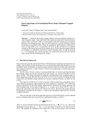
J. P. Leahy et al.: <strong>Planck</strong> pre-launch status: Expected LFI polarisation capabilitysystem. The astronomical convention 2 takes ˆx as due north (thelocal meridian) and ŷ along the local parallel towards the east,consistent with propagation (ẑ) towardstheobserver.Itisalsonecessary to specify which coordinate system is intended, viz.equatorial, ecliptic or galactic, and for the first two the referenceequinox (e.g. J2000 or date of observation). Many analyses ofCMB polarisation adopt the opposite handedness, resulting in achange of sign of U and Θ.Inthispaperweusetheastronomicalconvention throughout.To describe the instrumental polarisation properties, we alsoneed coordinate systems fixed with respect to the instrument.<strong>Planck</strong> is conventionally described by a Cartesian “spacecraft”frame in which the telescope is mirror-symmetric across theX SC Z SC plane, with the ray from the centre of the focal planeoriented at 85 ◦ from ˆX SC towards Ẑ SC .Inflight,thetelescopespins at f spin ≈ 1rpm,withitsspinvectornominallyparallelto ˆX SC and kept close to the anti-Sun direction. Hence the detectorbeams scan the sky along nearly-great circles, which aremost conveniently described as parallels in a coordinate frametaking the spin axis as its pole; we refer to this as the ZS frame(mnemonic that Ẑ ZS = ˆX SC is the spin axis). We specify thepolarisation orientation of the detectors, ψ,relativetothemeridiansof the ZS frame, and define the rotation of this orientationrelative to the celestial meridian in the pointing direction as χ(Fig. 1).Finally, the radiation pattern (“beam”) of each feed horn, afterfolding through the telescope optics, is defined using a variant3 of Ludwig’s 3rd definition of coordinates (Ludwig 1973)rather than polar coordinates, with the origin taken as the peakof the beam and orientated so that the co-polar axis is parallelto the projected polarisation of the “side-arm” radiometer (seeSect. 3.1)atthebeampeak(Sandri et al. 2010). Fortunately, thesky regions covered by the main beam patterns are small enoughthat we may use the flat-sky approximation when integrating thepolarisation response over the main beam.3. LFI polarimeter architecture3.1. Differencing polarimeter conceptThe output signal power produced by a linear, narrow-band detectorobserving a polarised source can be written in terms of thesource Stokes parameters as:P = Γ (I +Λ(Q cos 2θ + U sin 2θ) + ξV) (5)2(e.g. Kraus 1966). Here Γ is a gain factor, Λ is the linear polarisationefficiency (“polefficiency”), θ = ψ + χ is the detectorpolarisation orientation in the coordinates used to define (Q, U),and ξ represents the response to circular polarisation. The factorof 1/2 isincludedforlaterconvenience.Notethatθ givesthe orientation of the detector, while Θ in Eqs. (2) and(3) isforthe incoming radiation; evidently the response is ∝ cos 2(Θ − θ).Equation (5) appliestobothcoherentandincoherentdetectors(such as bolometers). We also have Λ 2 + ξ 2 ≤ 1, with equality2 As resolved by the IAU (Heeschen & Howard 1974). They specifythat Stokes parameters should be defined with respect to equatorial coordinates,which is too limiting in the current context, but we prefer toavoid the confusion caused by reversing the sense of position angle. Seealso Hamaker & Bregman (1996).3 We use the convention of the GRASP software (Pontoppidan 2005)that the co-polar component is parallel to ˆx in the vicinity of the mainbeam, whereas Ludwig (1973) haditparalleltoŷ.Fig. 1. Geometry of spin axis (red arrow directed away from the Sun)and scan line illustrated on a view of the celestial sphere. The northecliptic pole is marked NEP and the vernal point, i.e. the origin of (λ, β),is marked ♈. InblackareshowntheEcliptic,theprimeeclipticmeridian,and the parallel and meridian of the pixel with ecliptic longitudeand latitude (λ, β). In red are shown features fixed in ZS coordinates:the scan circle, with an arrow indicating the direction the detectors scanover the sky, the scan circle radius ρ, andthepolarisationorientation(double-headed arrow rotated by ψ relative to the ZS meridian). The positionangle offset χ between ecliptic and ZS coordinates for the markedpixel is also shown. Note that χ and ψ are measured anticlockwise asseen from inside the celestial sphere.Table 1. Geometric parameters for the LFI focal plane.Horn Band ρ a φ b ψ cLead Trail Side MainLFI-18 LFI-23 70 GHz 87. ◦ 20 2. ◦ 46 −22. ◦ 03 67. ◦ 67LFI-19 LFI-22 70 GHz 87. ◦ 77 1. ◦ 55 −22. ◦ 30 67. ◦ 70LFI-20 LFI-21 70 GHz 88. ◦ 10 0. ◦ 63 −22. ◦ 36 67. ◦ 74LFI-24 44 GHz 89. ◦ 05 0. ◦ 00 0. ◦ 00 90. ◦ 00LFI-26 LFI-25 44 GHz 82. ◦ 59 4. ◦ 43 −112. ◦ 52 −23. ◦ 32LFI-28 LFI-27 30 GHz 88. ◦ 90 1. ◦ 93 −22. ◦ 20 67. ◦ 50Notes. (a) Scan circle radius (ZS co-latitude); (b) phase along scan circle(ZS longitude); (c) polarisation orientation relative to ZS meridians (SeeFig. 1), using the astronomical sign convention (positive from north toeast). Note that the ψ MB listed by Sandri et al. (2010) useadifferentgeometrical definition. We only quote parameters for the leading hornin each matched pair: the values of φ and ψ for the trailing horn are thenegatives of those quoted.holding for a lossless coherent detector. Any detector comprisespart of an optical system (e.g. telescope) and the detector parametersΓ, Λ, θ and ξ will be functions of frequency ν and sourcedirection ˆn via the beam. In addition, they are functions of frequencybut not direction due to internal components such as filterswithin the detector. In Sect. 4.1, weshowhowEq.(5) canbe computed from the Jones matrices of individual componentsin the receiver chain.Page 3 of 26
- Page 1 and 2:
A&A 520, E1 (2010)DOI: 10.1051/0004
- Page 3 and 4:
ABSTRACTThe European Space Agency
- Page 5 and 6:
A&A 520, A1 (2010)Fig. 2. An artist
- Page 7 and 8:
A&A 520, A1 (2010)Fig. 4. Planck fo
- Page 9 and 10:
A&A 520, A1 (2010)Fig. 6. The Planc
- Page 11 and 12:
A&A 520, A1 (2010)Table 4. Summary
- Page 13 and 14:
A&A 520, A1 (2010)three frequency c
- Page 15 and 16:
A&A 520, A1 (2010)Fig. 12. The left
- Page 17 and 18:
A&A 520, A1 (2010)Fig. 14. Left pan
- Page 19 and 20:
A&A 520, A1 (2010)flux limit of the
- Page 21 and 22:
A&A 520, A1 (2010)- University of C
- Page 23 and 24:
A&A 520, A1 (2010)57 Instituto de A
- Page 25 and 26:
A&A 520, A2 (2010)Fig. 1. (Left) Th
- Page 27 and 28:
A&A 520, A2 (2010)Fig. 3. (Top)Twos
- Page 29 and 30:
A&A 520, A2 (2010)Table 2. Predicte
- Page 31 and 32:
Table 3. Predicted in-flight main b
- Page 33 and 34:
A&A 520, A2 (2010)materials. Theref
- Page 35 and 36:
A&A 520, A2 (2010)Fig. 11. Comparis
- Page 37 and 38:
A&A 520, A2 (2010)Table 5. Inputs u
- Page 39 and 40:
A&A 520, A2 (2010)Fig. 16. Three cu
- Page 41 and 42:
A&A 520, A2 (2010)Table 7. Optical
- Page 43 and 44:
A&A 520, A2 (2010)Fig. A.1. Dimensi
- Page 45 and 46:
A&A 520, A2 (2010)5 Università deg
- Page 47 and 48:
A&A 520, A3 (2010)Horizon 2000 medi
- Page 49 and 50:
A&A 520, A3 (2010)Fig. 1. CMB tempe
- Page 51 and 52:
A&A 520, A3 (2010)Ω ch 2τn s0.130
- Page 53 and 54:
A&A 520, A3 (2010)Fig. 6. Integral
- Page 55 and 56:
A&A 520, A3 (2010)Table 2. LFI opti
- Page 57 and 58:
3.3.1. SpecificationsThe main requi
- Page 59 and 60:
A&A 520, A3 (2010)Fig. 11. Schemati
- Page 61 and 62:
A&A 520, A3 (2010)features of the r
- Page 63 and 64:
A&A 520, A3 (2010)Fig. 13. Level 2
- Page 65 and 66:
A&A 520, A3 (2010)Fig. 15. Level 3
- Page 67 and 68:
A&A 520, A3 (2010)GUI = graphical u
- Page 69 and 70:
A&A 520, A3 (2010)23 Centre of Math
- Page 71 and 72:
A&A 520, A4 (2010)In addition, all
- Page 73 and 74:
A&A 520, A4 (2010)Table 2. Sensitiv
- Page 75 and 76:
A&A 520, A4 (2010)Fig. 2. Schematic
- Page 77 and 78:
A&A 520, A4 (2010)Fig. 6. LFI recei
- Page 79 and 80:
A&A 520, A4 (2010)Fig. 9. Schematic
- Page 81 and 82:
A&A 520, A4 (2010)Table 4. Specific
- Page 83 and 84: A&A 520, A4 (2010)Fig. 15. DAE bias
- Page 85 and 86: A&A 520, A4 (2010)Fig. 19. Picture
- Page 87 and 88: A&A 520, A4 (2010)Table 10. Main ch
- Page 89 and 90: Table 13. Principal requirements an
- Page 91 and 92: A&A 520, A5 (2010)DOI: 10.1051/0004
- Page 93 and 94: A. Mennella et al.: LFI calibration
- Page 95 and 96: A. Mennella et al.: LFI calibration
- Page 97 and 98: A. Mennella et al.: LFI calibration
- Page 99 and 100: A. Mennella et al.: LFI calibration
- Page 101 and 102: A. Mennella et al.: LFI calibration
- Page 103 and 104: A. Mennella et al.: LFI calibration
- Page 105 and 106: D.1. Step 1-extrapolate uncalibrate
- Page 107 and 108: A&A 520, A6 (2010)DOI: 10.1051/0004
- Page 109 and 110: F. Villa et al.: Calibration of LFI
- Page 111 and 112: F. Villa et al.: Calibration of LFI
- Page 113 and 114: F. Villa et al.: Calibration of LFI
- Page 115 and 116: F. Villa et al.: Calibration of LFI
- Page 117 and 118: F. Villa et al.: Calibration of LFI
- Page 119 and 120: F. Villa et al.: Calibration of LFI
- Page 121 and 122: A&A 520, A7 (2010)DOI: 10.1051/0004
- Page 123 and 124: M. Sandri et al.: Planck pre-launch
- Page 126 and 127: A&A 520, A7 (2010)Fig. 8. Footprint
- Page 128 and 129: -30-40-30-6-3-20A&A 520, A7 (2010)0
- Page 130 and 131: A&A 520, A7 (2010)Table 4. Galactic
- Page 132 and 133: A&A 520, A7 (2010)Fig. A.1. Polariz
- Page 136 and 137: A&A 520, A8 (2010)estimated from th
- Page 138 and 139: A&A 520, A8 (2010)ways the most str
- Page 140 and 141: unmodelled long-timescale thermally
- Page 142 and 143: A&A 520, A8 (2010)Fig. 5. Polarisat
- Page 144 and 145: A&A 520, A8 (2010)Table 3. Band-ave
- Page 146 and 147: A&A 520, A8 (2010)where S stands fo
- Page 148 and 149: A&A 520, A8 (2010)Fig. 11. Simulate
- Page 150 and 151: stored in the LFI instrument model,
- Page 152 and 153: A&A 520, A8 (2010)Table 5. Statisti
- Page 154 and 155: A&A 520, A8 (2010)comparable in siz
- Page 156 and 157: A&A 520, A8 (2010)Table B.1. Main b
- Page 158 and 159: A&A 520, A8 (2010)Bond, J. R., Jaff
- Page 160 and 161: A&A 520, A9 (2010)- (v) an optical
- Page 162 and 163: A&A 520, A9 (2010)Fig. 2. The Russi
- Page 164 and 165: A&A 520, A9 (2010)Table 3. Estimate
- Page 166 and 167: A&A 520, A9 (2010)Fig. 7. Picture o
- Page 168 and 169: A&A 520, A9 (2010)Fig. 9. Cosmic ra
- Page 170 and 171: A&A 520, A9 (2010)Fig. 13. Principl
- Page 172 and 173: A&A 520, A9 (2010)Fig. 16. Noise sp
- Page 174 and 175: A&A 520, A9 (2010)Table 6. Basic ch
- Page 176 and 177: A&A 520, A9 (2010)with warm preampl
- Page 178 and 179: A&A 520, A9 (2010)20 Laboratoire de
- Page 180 and 181: A&A 520, A10 (2010)Table 1. HFI des
- Page 182 and 183: A&A 520, A10 (2010)based on the the
- Page 184 and 185:
A&A 520, A10 (2010)Fig. 6. The Satu
- Page 186 and 187:
A&A 520, A10 (2010)5. Calibration a
- Page 188 and 189:
A&A 520, A10 (2010)Fig. 16. Couplin
- Page 190 and 191:
A&A 520, A10 (2010)217-5a channel:
- Page 192 and 193:
A&A 520, A10 (2010)10 -310 -495-The
- Page 194 and 195:
A&A 520, A11 (2010)DOI: 10.1051/000
- Page 196 and 197:
P. A. R. Ade et al.: Planck pre-lau
- Page 198 and 199:
P. A. R. Ade et al.: Planck pre-lau
- Page 200 and 201:
P. A. R. Ade et al.: Planck pre-lau
- Page 202 and 203:
A&A 520, A12 (2010)Table 1. Summary
- Page 204 and 205:
arrangement was also constrained by
- Page 206 and 207:
A&A 520, A12 (2010)frequency cut-of
- Page 208 and 209:
A&A 520, A12 (2010)Fig. 9. Gaussian
- Page 210 and 211:
A&A 520, A12 (2010)the horn-to-horn
- Page 212 and 213:
A&A 520, A12 (2010)Fig. 15. Composi
- Page 214 and 215:
A&A 520, A12 (2010)Fig. 19. Broad-b
- Page 216 and 217:
A&A 520, A13 (2010)DOI: 10.1051/000
- Page 218 and 219:
C. Rosset et al.: Planck-HFI: polar
- Page 220 and 221:
C. Rosset et al.: Planck-HFI: polar
- Page 222 and 223:
of frequencies and shown to have po
- Page 224 and 225:
C. Rosset et al.: Planck-HFI: polar
- Page 226 and 227:
C. Rosset et al.: Planck-HFI: polar