Planck Pre-Launch Status Papers - APC - Université Paris Diderot ...

A&A 520, E1 (2010)DOI: 10.1051/0004-6361/201015611c○ ESO 2010Pre-launch status of the Planck missionAstronomy&AstrophysicsSpecial featureEditorialPre-launch status of the Planck missionThis A&A issue features 13 articles describingthepre-flightstatus of the European Space Agency Planck mission, launchedtogether with the Herschel satellite on 14 May 2009. The Planck mission is designed to image the anisotropies of the cosmicbackground radiation field over the whole sky, with unprecedented sensitivity and angular resolution, as well as a wide frequencyrange. As a byproduct of that main goal, it will simultaneously address a wide range of galactic and extragalactic science. Themission involves more than four hundred scientists, who are currently working on data processing, calibration, and data analysis.The satellite is scheduled to continuously acquire high-quality science data until the end of 2011. An early release of the compactsource catalogue will be delivered in January 2011, together with a small set of science papers related to foreground astrophysicalsources. The first major cosmology results will be delivered in December 2012.In this special feature, the telescope’s optical system and the design, ground calibration, and performance of the Planck lowandhigh-frequency instruments are described in detail.C. Bertout and T. ForveilleAstronomy & Astrophysics EditorsArticle published by EDP Sciences Page 1 of 1

A&A 520, A1 (2010)DOI: 10.1051/0004-6361/200912983c○ ESO 2010Pre-launch status of the Planck missionAstronomy&AstrophysicsSpecial featurePlanck pre-launch status: The Planck missionJ. A. Tauber 36 ,N.Mandolesi 45 ,J.-L.Puget 52 ,T.Banos 82 ,M.Bersanelli 32 ,F.R.Bouchet 51 ,R.C.Butler 45 ,J.Charra 52 ,G.Crone 37 ,J. Dodsworth 38 ,G.Efstathiou 90 ,R.Gispert 52 ,G.Guyot 52 ,A.Gregorio 93 ,J.J.Juillet 82 ,J.-M.Lamarre 66 ,R.J.Laureijs 36 ,C.R.Lawrence 61 ,H. U. Nørgaard-Nielsen 35 ,T.Passvogel 37 ,J.M.Reix 82 ,D.Texier 39 ,L.Vibert 52 ,A.Zacchei 46 ,P.A.R.Ade 6 ,N.Aghanim 52 ,B.Aja 18 ,E.Alippi 84 ,L. Aloy 37 ,P.Armand 82 ,M.Arnaud 7 ,A.Arondel 52 ,A.Arreola-Villanueva 61 ,E.Artal 18 ,E.Artina 84 ,A.Arts 37 ,M.Ashdown 89 ,J.Aumont 9 ,M. Azzaro 40 ,A.Bacchetta 83 ,C.Baccigalupi 5 ,M.Baker 37 ,M.Balasini 84 ,A.Balbi 33 ,A.J.Banday 67,12 ,G.Barbier 64 ,R.B.Barreiro 58 ,M. Bartelmann 67,95 ,P.Battaglia 84 ,E.Battaner 91 ,K.Benabed 51 ,J.-L.Beney 63 ,R.Beneyton 51 ,K.Bennett 36 ,A.Benoit 64 ,J.-P.Bernard 12 ,P. Bhandari 61 ,R.Bhatia 61 ,M.Biggi 74 ,R.Biggins 38 ,G.Billig 38 ,Y.Blanc 14 ,H.Blavot 52 ,J.J.Bock 61 ,A.Bonaldi 49 ,R.Bond 13 ,J.Bonis 63 ,J. Borders 61 ,J.Borrill 88 ,L.Boschini 84 ,F.Boulanger 52 ,J.Bouvier 64 ,M.Bouzit 52 ,R.Bowman 61 ,E.Bréelle 4 ,T.Bradshaw 77 ,M.Braghin 37 ,M. Bremer 36 ,D.Brienza 34 ,D.Broszkiewicz 4 ,C.Burigana 45 ,M.Burkhalter 73 ,P.Cabella 33 ,T.Cafferty 61 ,M.Cairola 83 ,S.Caminade 52 ,P. Camus 53 ,C.M.Cantalupo 65 ,B.Cappellini 32 ,J.-F.Cardoso 4 ,R.Carr 39 ,A.Catalano 4 ,L.Cayón 23 ,M.Cesa 83 ,M.Chaigneau 52 ,A.Challinor 90 ,A. Chamballu 43 ,J.P.Chambelland 82 ,M.Charra 52 ,L.-Y.Chiang 55 ,G.Chlewicki 83 ,P.R. Christensen 71 ,S.Church 24 ,E.Ciancietta 83 ,M. Cibrario 83 ,R.Cizeron 63 ,D.Clements 43 ,B.Collaudin 82 ,J.-M.Colley 4,51 ,S.Colombi 51 ,A.Colombo 37 ,F.Colombo 84 ,O.Corre 82 ,F. Couchot 63 ,B.Cougrand 52 ,A.Coulais 66 ,P.Couzin 82 ,B.Crane 52 ,B.Crill 61 ,M.Crook 77 ,D.Crumb 61 ,F. Cuttaia 45 ,U.Dörl 67 ,P.daSilva 51 ,R. Daddato 37 ,C.Damasio 37 ,L.Danese 5 ,G.d’Aquino 37 ,O.D’Arcangelo 60 ,K.Dassas 52 ,R.D.Davies 62 ,W.Davies 73 ,R.J.Davis 62 ,P. De Bernardis 34 ,D.deChambure 37 ,G.deGasperis 33 ,M.L.DelaFuente 18 ,P.DePaco 81 ,A.DeRosa 45 ,G.DeTroia 33 ,G.DeZotti 49 ,M. Dehamme 63 ,J.Delabrouille 4 ,J.-M.Delouis 51 ,F.-X.Désert 64 ,G.diGirolamo 38 ,C.Dickinson 62 ,E.Doelling 38 ,K.Dolag 67 ,I.Domken 11 ,M. Douspis 52 ,D.Doyle 37 ,S.Du 63 ,D.Dubruel 82 ,C.Dufour 4 ,C.Dumesnil 52 ,X.Dupac 39 ,P.Duret 52 ,C.Eder 63 ,A.Elfving 37 ,T.A.Enßlin 67 ,P. Eng 52 ,K.English 61 ,H.K.Eriksen 10,56 ,P.Estaria 37 ,M.C.Falvella 2 ,F.Ferrari 84 ,F.Finelli 45 ,A.Fishman 61 ,S.Fogliani 46 ,S.Foley 38 ,A. Fonseca 61 ,G.Forma 82 ,O.Forni 12 ,P.Fosalba 87 ,J.-J.Fourmond 52 ,M.Frailis 46 ,C.Franceschet 32 ,E.Franceschi 45 ,S.François 52 ,M. Frerking 61 ,M.F.Gómez-Reñasco 57 ,K.M.Górski 61 ,T.C.Gaier 61 ,S.Galeotta 48 ,K.Ganga 4 ,J.GarcíaLázaro 39 ,A.Garnica 61 ,M.Gaspard 63 ,E. Gavila 82 ,M.Giard 12 ,G.Giardino 36 ,G.Gienger 38 ,Y.Giraud-Heraud 4 ,J.-M.Glorian 12 ,M.Griffin 6 ,A.Gruppuso 45 ,L.Guglielmi 4 ,D. Guichon 82 ,B.Guillaume 37 ,P.Guillouet 4 ,J.Haissinski 63 ,F.K.Hansen 10,56 ,J.Hardy 61 ,D.Harrison 90 ,A.Hazell 76 ,M.Hechler 38 ,V. Heckenauer 52 ,D.Heinzer 38 ,R.Hell 67 ,S.Henrot-Versillé 63 ,C.Hernández-Monteagudo 67 ,D.Herranz 58 ,J.M.Herreros 57 ,V.Hervier 52 ,A. Heske 37 ,A.Heurtel 63 ,S.R.Hildebrandt 57 ,R.Hills 89 ,E.Hivon 51 ,M.Hobson 89 ,D.Hollert 61 ,W.Holmes 61 ,A.Hornstrup 35 ,W.Hovest 67 ,R. J. Hoyland 57 ,G.Huey 61 ,K.M.Huffenberger 92 ,N.Hughes 94 ,U.Israelsson 61 ,B.Jackson 37 ,A.Jaffe 43 ,T.R.Jaffe 62 ,T.Jagemann 39 ,N. C. Jessen 35 ,J.Jewell 61 ,W.Jones 22 ,M.Juvela 72 ,J.Kaplan 4 ,P.Karlman 61 ,F.Keck 38 ,E.Keihänen 21 ,M.King 61 ,T.S.Kisner 65 ,P.Kletzkine 37 ,R. Kneissl 67 ,J.Knoche 67 ,L.Knox 26 ,T.Koch 61 ,M.Krassenburg 37 ,H.Kurki-Suonio 21,42 ,A.Lähteenmäki 68 ,G.Lagache 52 ,E.Lagorio 64 ,P. Lami 52 ,J.Lande 12 ,A.Lange 61 ,F.Langlet 52 ,R.Lapini 74 ,M.Lapolla 84 ,A.Lasenby 89 ,M.LeJeune 4 ,J.P.Leahy 62 ,M.Lefebvre 52 ,F. Legrand 51 ,G.LeMeur 63 ,R.Leonardi 27 ,B.Leriche 52 ,C.Leroy 52 ,P.Leutenegger 84 ,S.M.Levin 61 ,P.B.Lilje 10,56 ,C.Lindensmith 61 ,M. Linden-Vørnle 86 ,A.Loc 61 ,Y.Longval 52 ,P.M.Lubin 27 ,T.Luchik 61 ,I.Luthold 37 ,J.F.Macias-Perez 96 ,T.Maciaszek 14 ,C.MacTavish 43 ,S. Madden 37 ,B.Maffei 62 ,C.Magneville 8 ,D.Maino 32 ,A.Mambretti 84 ,B.Mansoux 63 ,D.Marchioro 84 ,M.Maris 46 ,F.Marliani 37 ,J.-C. Marrucho 63 ,J.Martí-Canales 37 ,E.Martínez-González 58 ,A.Martín-Polegre 37 ,P.Martin 82 ,C.Marty 12 ,W.Marty 12 ,S.Masi 34 ,M. Massardi 49 ,S.Matarrese 31 ,F.Matthai 67 ,P.Mazzotta 33 ,A.McDonald 38 ,P.McGrath 61 ,A.Mediavilla 18 ,P.R.Meinhold 27 ,J.-B.Mélin 8 ,F. Melot 96 ,L.Mendes 39 ,A.Mennella 32 ,C.Mervier 52 ,L.Meslier 52 ,M.Miccolis 84 ,M.-A.Miville-Deschenes 52 ,A.Moneti 51 ,D.Montet 82 ,L. Montier 12 ,J.Mora 61 ,G.Morgante 45 ,G.Morigi 45 ,G.Morinaud 52 ,N.Morisset 59 ,D.Mortlock 90 ,S.Mottet 51 ,J.Mulder 61 ,D.Munshi 90 ,A. Murphy 70 ,P.Murphy 61 ,P.Musi 83 ,J.Narbonne 12 ,P. Naselsky 71 ,A.Nash 61 ,F.Nati 34 ,P.Natoli 33 ,B.Netterfield 13 ,J.Newell 61 ,M.Nexon 12 ,C. Nicolas 52 ,P.H.Nielsen 85 ,N.Ninane 11 ,F.Noviello 52 ,D.Novikov 43 ,I.Novikov 71 ,I.J.O’Dwyer 61 ,P.Oldeman 37 ,P.Olivier 37 ,L.Ouchet 82 ,C. A. Oxborrow 35 ,L.Pérez-Cuevas 37 ,L.Pagan 84 ,C.Paine 61 ,F.Pajot 52 ,R.Paladini 80 ,F.Pancher 64 ,J.Panh 14 ,G.Parks 61 ,P.Parnaudeau 51 ,B. Partridge 41 ,B.Parvin 61 ,J.P.Pascual 18 ,F.Pasian 46 ,D.P.Pearson 61 ,T.Pearson 61 ,M.Pecora 84 ,O.Perdereau 63 ,L.Perotto 96 ,F.Perrotta 5 ,F. Piacentini 34 ,M.Piat 4 ,E.Pierpaoli 20 ,O.Piersanti 37 ,E.Plaige 63 ,S.Plaszczynski 63 ,P.Platania 60 ,E.Pointecouteau 12 ,G.Polenta 1 ,N. Ponthieu 52 ,L.Popa 54 ,G.Poulleau 52 ,T.Poutanen 21,42,68 ,G.Prézeau 61 ,L.Pradell 16 ,M.Prina 61 ,S.Prunet 51 ,J.P.Rachen 67 ,D.Rambaud 12 ,F. Rame 83 ,I.Rasmussen 37 ,J.Rautakoski 37 ,W.T.Reach 50 ,R.Rebolo 57 ,M.Reinecke 67 ,J.Reiter 61 ,C.Renault 96 ,S.Ricciardi 79 ,P.Rideau 82 ,T. Riller 67 ,I.Ristorcelli 12 ,J.B.Riti 82 ,G.Rocha 61 ,Y.Roche 82 ,R.Pons 12 ,R.Rohlfs 59 ,D.Romero 61 ,S.Roose 11 ,C.Rosset 63 ,S.Rouberol 51 ,M. Rowan-Robinson 43 ,J.A.Rubiño-Martín 57 ,P.Rusconi 84 ,B.Rusholme 50 ,M.Salama 61 ,E.Salerno 15 ,M.Sandri 45 ,D.Santos 96 ,J.L.Sanz 58 ,L. Sauter 51 ,F.Sauvage 82 ,G.Savini 75 ,M.Schmelzel 61 ,A.Schnorhk 37 ,W.Schwarz 61 ,D.Scott 19 ,M.D.Seiffert 61 ,P.Shellard 89 ,C.Shih 61 ,M. Sias 83 ,J.I.Silk 29 ,R.Silvestri 84 ,R. Sippel 3 ,G.F.Smoot 25 ,J.-L.Starck 8 ,P.Stassi 96 ,J.Sternberg 36 ,F.Stivoli 79 ,V.Stolyarov 90 ,R.Stompor 4 ,L. Stringhetti 45 ,D.Strommen 61 ,T.Stute 3 ,R.Sudiwala 6 ,R.Sugimura 61 ,R.Sunyaev 67 ,J.-F.Sygnet 51 ,M.Türler 59 ,E.Taddei 84 ,J.Tallon 61 ,C. Tamiatto 52 ,M.Taurigna 63 ,D.Taylor 39 ,L.Terenzi 45 ,S.Thuerey 37 ,J.Tillis 61 ,G.Tofani 44 ,L.Toffolatti 17 ,E.Tommasi 2 ,M.Tomasi 32 ,E. Tonazzini 15 ,J.-P.Torre 52 ,S.Tosti 52 ,F.Touze 63 ,M.Tristram 63 ,J.Tuovinen 69 ,M.Tuttlebee 38 ,G.Umana 47 ,L.Valenziano 45 ,D.Vallée 4 ,M. van der Vlis 37 ,F.VanLeeuwen 90 ,J.-C.Vanel 4 ,B.Van-Tent 51 ,J.Varis 69 ,E.Vassallo 38 ,C.Vescovi 64 ,F.Vezzu 64 ,D.Vibert 51 ,P.Vielva 58 ,J. Vierra 61 ,F.Villa 45 ,N.Vittorio 33 ,C.Vuerli 46 ,L.A.Wade 61 ,A.R.Walker 19 ,B.D.Wandelt 28 ,C.Watson 38 ,D.Werner 38 ,M.White 30 ,S. D. M. White 67 ,A.Wilkinson 62 ,P.Wilson 61 ,A.Woodcraft 6 ,B.Yoffo 4 ,M.Yun 61 ,V.Yurchenko 70 ,D.Yvon 8 ,B.Zhang 61 ,O.Zimmermann 64 ,A. Zonca 48 ,andD.Zorita 78(Affiliations can be found after the references)Received 24 July 2009 / Accepted 12 November 2009Page 1 of 22

ABSTRACTThe European Space Agency’s Planck satellite, launched on 14 May 2009, is the third-generation space experiment in the field of cosmic microwavebackground (CMB) research. It will image the anisotropies of the CMB over the whole sky, with unprecedented sensitivity ( ∆T ∼ 2 ×T10 −6 )andangularresolution(∼5 arcmin).Planck will provide a major source of information relevant to many fundamental cosmological problemsand will test current theories of the early evolution of the Universe and the origin of structure. It will also address a wide range of areas ofastrophysical research related to the Milky Way as well as external galaxies and clustersofgalaxies.TheabilityofPlanck to measure polarizationacross a wide frequency range (30−350 GHz), with high precision and accuracy, and over the whole sky, will provide unique insight, not onlyinto specific cosmological questions, but also into the properties of the interstellar medium. This paper is part of a series which describes thetechnical capabilities of the Planck scientific payload. It is based on the knowledge gathered during the on-ground calibration campaigns of themajor subsystems, principally its telescope and its two scientific instruments, and of tests at fully integrated satellite level. It represents the bestestimate before launch of the technical performance that the satellite and its payload will achieve in flight. In this paper, we summarise the mainelements of the payload performance, which is described in detail in the accompanying papers. In addition, we describe the satellite performanceelements which are most relevant for science, and provide an overview of the plans for scientific operations and data analysis.Key words. cosmic microwave background – space vehicles: instruments – instrumentation: detectors – instrumentation: polarimeters –submillimeter: general – radio continuum: general1. IntroductionThe Planck mission 1 was conceived in 1992, in the wake of therelease of the results from the COsmic Background Explorer(COBE) satellite (Boggess et al. 1992), notably the measurementby the FIRAS instrument of the shape of the spectrum of thecosmic microwave background (CMB), and the detection by theDMR instrument of the spatial anisotropies of the temperatureof the CMB. The latter result in particular led to an explosionin the number of ground-based and suborbital experiments dedicatedto mapping of the anisotropies, and to proposals for spaceexperiments both in Europe and the USA.The development of Planck began with two proposalspresented to the European Space Agency (ESA) in Mayof 1993, for the COsmic Background Radiation AnisotropySatellite (COBRAS, Mandolesi et al. 1993) andtheSAtellitefor Measurement of Background Anisotropies (SAMBA, Pugetet al. 1993). Each of these proposed a payload formed by anoffset Gregorian telescope focussing light from the sky ontoan array of detectors (based on high electron mobility transistor[HEMT] low noise amplifiers for COBRAS and very lowtemperature bolometers for SAMBA) fed by corrugated horns.The two proposals were used by an ESA-led team to designapayloadwhereasingleCOBRAS-liketelescopefedtwoinstruments,a COBRAS-like Low Frequency Instrument (LFI),and a SAMBA-like High Frequency Instrument (HFI) sharingacommonfocalplane.Aperiodofstudyofthisconceptculminatedin the selection by ESA in 1996 of the COBRAS/SAMBAsatellite (described in the so-called “Redbook”, Bersanelli et al.1996) intoitsprogrammeofscientificsatellites.Atthetimeofselection the launch of COBRAS/SAMBA was expected to be in2003. Shortly after the mission was approved, it was renamed inhonor of the German scientist Max Planck (1858–1947), winnerof the Nobel Prize for Physics in 1918.Shortly after its selection, the development of Planck wasjoined with that of ESA’s Herschel Space Telescope, based onanumberofpotentialcommonalities,themostimportantofwhich was that both missions targeted orbits around the secondLagrangian point of the Sun-Earth system and could thereforeshare a single heavy launcher. In practice the joint development1 Planck (http://www.esa.int/Planck) is a project of theEuropean Space Agency – ESA – with instruments provided by two scientificConsortia funded by ESA member states (in particular the leadcountries: France and Italy) with contributions from NASA (USA), andtelescope reflectors provided in a collaboration between ESA and a scientificConsortium led and funded by Denmark.has meant that a single ESA engineering team has led the developmentof both satellites by a singleindustrialprimecontractor,leading to the use of many identical hardware and software subsystemsin both satellites, and a synergistic sharing of engineeringskills and manpower. The industrial prime contractor, ThalesAlenia Space France, was competitively selected in early 2001.Thales Alenia Space France was supported by two major subcontractors:Thales Alenia Space Italy for the service module ofboth Planck and Herschel, andEADSAstriumGmbHfortheHerschel payload module, and by many other industrial subcontractorsfrom all ESA member states. The development of thesatellite has been regularly reported over the years, see e.g. Reixet al. (2007).In early 1999, ESA selected two consortia of scientific institutesto provide the two Planck instruments which were partof the payload described in the Redbook: the LFI was developedby a consortium led by N. Mandolesi of the Istituto diAstrofisica Spaziale e Fisica Cosmica (CNR) in Bologna (Italy);and the HFI by a consortium led by J.-L. Puget of the Institutd’Astrophysique Spatiale (CNRS) in Orsay (France). More than40 European institutes, and some from the USA, have collaboratedon the development and testing of these instruments, andwill continue to carry out their operation, as well as the ensuingdata analysis and initial scientific exploitation (see alsoAppendix A).In early 2000, ESA and the Danish National Space Institute(DNSI) signed a Letter of Agreement for the provision of thetwo reflectors that are used in the Planck telescope. DNSI led aconsortium of Danish institutes, which together with ESA subcontractedthe development of the Planck reflectors to EADSAstrium GmbH (Friedrichshafen, D), who have manufacturedthe reflectors using state-of-the-art carbon fibre technology.The long development history of the Planck satellite (seeFig. 1)culminatedwithitssuccessfullaunchon14May2009.This paper is not meant to describe in detail Planck’s scientificobjectives or capabilities. A detailed and still quite upto-datedescription of the Planck mission and, more specifically,of its scientific objectives was produced in 2005, the“Planck Bluebook” (Planck Collaboration 2005). This paper ismeant to provide an update to the technical description of thepayload in the Planck Bluebook, summarisingthebestknowledgeavailable at the time of launch of the major scientificallyrelevant performance elements of the satellite and its payload,based on all the ground testing activities and extrapolation toflight conditions. It is part of a set of papers which details thepayload performance and which will be referred to whenever

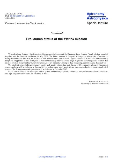
J. A. Tauber et al.: Planck pre-launch status: The Planck mission2. Satellite descriptionFigures 2 and 3 show the major elements and characteristics ofthe Planck satellite. Planck was designed, built and tested aroundtwo major modules:1. a payload module (see Fig. 5) containinganoff-axis telescopewith a projected diameter of 1.5 m, focussing radiationfrom the sky onto a focal plane shared by detectors of the LFIand HFI, operating at 20 K and 0.1 K respectively; a telescopebaffle thatsimultaneouslyprovidesstray-lightshieldingand radiative cooling; and three conical “V-groove” bafflesthat provide thermal and radiative insulation between thewarm service module and the cold telescope and instruments.2. a service module (see Fig. 6) containingallthewarmelectronicsservicing instruments and satellite; and the solarpanel providing electrical power. It also contains the cryocoolers,the main on-board computer, the telecommand receiversand telemetry transmitters, and the attitude controlsystem with its sensors and actuators.The most relevant technical characteristics of the Planck spacecraftare detailed in Table 1.Fig. 1. The fully assembled Planck satellite a few days before integrationinto the Ariane 5 rocket. Herschel is visible by reflection on theprimary reflector. Photo by A. Arts.possible for detailed descriptions. In addition to a summary ofthe material presented in the accompanying papers, this one alsoincludes a description of the scientifically relevant elements ofthe satellite performance, of its planned operations, and a briefoverview of the “science ground segment”. The main accompanyingpapers, most of which are part of this special issue ofAstronomy & Astrophysics,include:– Tauber et al. (2010), describing the optical performance ofthe combined payload, i.e. telescope plus instruments;– Mandolesi et al. (2010), describing programmatic aspects ofthe LFI and its development;– Bersanelli et al. (2010), describing in detail the design of theLFI;– Mennella et al. (2010), describing the test and calibrationprogramme of the LFI at instrument and system levels priorto launch;– Villa et al. (2010), describing the test and calibration of theLFI radiometer chains;– Sandri et al. (2010), describing the design and test of the LFIoptics;– Leahy et al. (2010), describing the polarisation aspects of theLFI, and its expected performance in orbit;– Lamarre et al. (2010), describing in detail the on-ground design,manufacture, test and performance of the HFI;– Pajot et al. (2010), describing the test and calibration programmeof the HFI prior to launch;– Ade et al. (2010), describing the design, test and performanceof the cryogenic elements of the HFI focal plane;– Holmes et al. (2008), describing the design, manufacture andtest of the HFI bolometers;– Maffei et al. (2010), describing the design and test of the HFIoptics;– Rosset et al. (2010), describing the polarisation aspects ofthe HFI.2.1. PointingPlanck spins at 1 rpm around the axis of symmetry of the solarpanel 2 .Inflight,thesolarpanelcanbepointedwithinaconeof 10 ◦ around the direction to the Sun; everything else is alwaysin its shadow. The attitude control system relies principally on:– Redundant star trackers as main sensors, and solar cells forrough guidance and anomaly detection. The star trackerscontain CCDs which are read out in synchrony with thespeed of the field-of-view across the sky to keep star imagescompact.– Redundant sets of hydrazine 20 N thrusters for large manoeuversand 1 N thrusters for fine manoeuvers.An on-board computer dedicated to this task reads out the startrackers at a frequency of 4 Hz, and determines in real time theabsolute pointing of the satellite based on a catalogue of brightstars. Manoeuvers are carried out as a sequence of 3 or 4 thrustsspaced in time by integer spin periods, whose duration is calculatedon-board, with the objective to achieve the requested attitudewith minimal excitation of nutation. There is no further activedamping of nutation during periods of inertial pointing, i.e.between manoeuvers. The duration of a small manoeuver typicalof routine operations (2 arcmin) is ∼5 min.Largermanoeuversare achieved by a combination of thrusts using both 1 Nand 20 N thrusters, and their duration can be considerable (up toseveral hours for manoeuver amplitudes of several degrees). Theattitudes measured on-board are further filtered on the ground toreconstruct with high accuracy the spacecraft attitude (or ratherthe star tracker reference frame). The star trackers and the instrumentalfield-of-view were aligned on the ground independentlyto the spacecraft reference frame; the resulting alignmentaccuracy between the star trackers and the instruments was of2 In reality, Planck spins about its principal axis of inertia, whichdoes not coincide exactly with the geometrical axis; this difference willevolve slowly during the mission due to fuel expenditure. After ongroundbalancing, the difference (often called “wobble angle”) is predictedto be ∼–14 arcmins just after launch (mainly around the Y axis,see Fig. 3), and to vary between ∼–5 arcmins after the final injection manoeuverinto L2 (when most of the fuel has been expended), to ∼+5arcminat end of the nominal mission lifetime.Page 3 of 22

A&A 520, A1 (2010)Fig. 2. An artist’s impression of the main elements of Planck. Theinstrumentfocalplaneunit(barelyvisible,seeFig.4) containsbothLFIandHFI detectors. The function of the large baffle surroundingthetelescopeistocontrolthevery-far-sidelobeleveloftheradiationpatternasseenfrom the detectors, and it also contributes substantially to radiative cooling of the payload. The specular conical shields (often called “V-grooves”)thermally decouple the octagonal service module (whichcontainsallwarmelements of the satellite) from the payload module. The clampbandadapter which holds the satellite to the rocket,andthemedium-gainhornantennausedtotransmit science data to ground are also indicated.0. ◦ 19, far better than required. The angles between the star trackerframe and each of the detectors are determined in flight fromobservations of planets. Several bright planets drift through thefield-of-view once every 6 months, providing many calibrationpoints every year. There are many weaker point sources, bothcelestial and in the Solar System, which provide much more frequentthough less accurate calibration tests.Thein-flightpointingcalibration is very robust vis-à-vis the expected thermoelasticdeformations (which contribute a total of 0.14 arcmin to thetotal on-ground alignment budget). The most important pointingperformance aspects, based on a realistic simulation using ratherconservative parameter values, and tests of the attitude controlsystem, are summarised in Table 2.The 20 N thrusters are also used for orbit control manoeuversduring transfer to the final Planck orbit (two large manoeuversplanned) and for orbit maintenance (typically one manoeuver permonth). Most of the hydrazine thruster fuel that Planck carries isexpended in the two large manoeuvers carried out during transfer,and a very minor amount is required for orbit maintenance.2.2. Thermal design and the cryo-chainThe cryogenic temperatures required by the detectors areachieved through a combination of passive radiative cooling andthree active refrigerators. The contrast between the high powerdissipation in the warm service module (∼1000 W at 300 K) andthat at the coldest spot in the satellite (∼100 nW at 0.1 K) aretestimony to the extraordinary efficiency of the complex thermalsystem which has to achieve such disparate ends simultaneouslywhile preserving a very high level of stability at the cold end.The telescope baffleandV-grooveshields(seeFig.2)arekeyparts of the passive thermal system. The baffle (which also actsas a stray-light shield) is a high-efficiency radiator consisting of∼14 m 2 of open aluminium honeycomb coated with black cryogenicpaint; the effective emissivity of this combination is veryhigh (>0.9). The “V-grooves” are a set of three conical shieldswith an angle of 5 ◦ between adjacent shields; the surfaces (approx10 m 2 on each side) are specular (aluminum coating with anemissivity of ∼0.045) except for the outer (∼4.5 m 2 )areaofthetopmost V-groove which has the same high-emissivity coatingas the baffle. This geometry provides highly efficient radiativecoupling to cold space, and a high degree of thermal and radiativeisolation between the warm spacecraft bus and the cold telescope,baffle, and instruments. The cooling provided by the passivesystem leads to a temperature of 40–45 K for the telescopeand baffle. Table 3 lists temperature ranges predicted in flightfor various parts of the satellite, based on a thermo-mechanicalmodel which has been correlated to test results; the uncertaintyin the prediction for elements in the cold payload is of order(+0.5 K, −2K).The active refrigeration chain further reduces the detectortemperatures to 20 K (LFI front-end low noise amplifiers) and0.1 K (HFI bolometers) respectively. It is based on three distinctunits working in series (see Fig. 7):1. The hydrogen sorption cooler was designed and built expresslyfor Planck at NASA’s Jet Propulsion LaboratoryPage 4 of 22

J. A. Tauber et al.: Planck pre-launch status: The Planck missionFig. 3. Engineering cross-sectional diagrams of Planck show its overall dimensions (in mm). The satellite spins around the vertical axis (+X),such that the solar array is always exposed to the Sun, and shields the payload from solar radiation. The shadow cone (±10 ◦ )isindicatedintheleft panel; theTMcone(±15 ◦ ), i.e. the angle within which the medium-gain data transmission link to Earth can be maintained, is also indicated.Figures courtesy of Thales Alenia Space (France).Table 1. Planck satellite characteristics.Diameter 4.2 m Defined by the solar arrayHeight4.2 mTotal mass at launch 1912 kg Fuel mass = 385 kg at launch; He mass = 7.7 kgElectrical power demand (avg) 1300 W Instrument part: 685 W (Begining of Life), 780 W (End of Life)Operational lifetime 18 months Plus a possible extension of one yearSpin rate 1 rpm ±0.6 arcmin/sec (changes due to manoeuvers)Stability during inertial pointing ∼ 6.5 × 10 −5 rpm/hMax angle of spin axis to Sun 10 ◦ To maintain the payload in the shade. Default angle is 7. ◦ 5.Max angle of spin axis to Earth 15 ◦ To allow communication to EarthAngle between spin axis and telescope boresight 85 ◦ Max extent of FOV ∼ 8 ◦On-board data storage capacity 32 Gbit Two redundant units (only one is operational at any time)Data transmission rate to ground (max) 1.5 Mbps Within 15 ◦ of Earth, using a 35 m ground antennaDaily contact period 3 h The effective real-time science data acquisition bandwidth is 130 kbps.(USA) (Bhandari et al. 2004; Pearsonetal.2006); it directlycools the LFI low-noise amplifiers to their operatingtemperature while providing pre-cooling for the HFIcooler chain. The sorption cooler consists of two cold redundantunits, each including a six-element sorption compressorand a Joule-Thomson (JT) expansion valve. Eachelement of the compressor is filled with hydride material(La Ni 4.78 Sn 0.22 )whichalternatelyabsorbsandreleaseshydrogengas under control of a heat source. The cooler producesliquid hydrogen in two liquid-vapor heat-exchangers(LVHXs) whose temperatures are stabilized by hydrogen absorptioninto three compressor elements. LVHX1 providespre-cooling for the HFI 4K cooler, while LVHX2 cools theLFI focal plane unit (FPU). The vapor pressure of the liquidhydrogen in the LVHXs is determined primarily by the absorptionisotherms of the hydride material used in the compressorelements. Thus, the heat rejection temperature ofthe compressor elements determines the instrument temperatures.On the spacecraft the compressor rejects heat to aradiator to space with flight allowable temperatures between262 and 282 K; the radiator is a single unit whichcouples the active and redundant sorption coolers via a networkof heat pipes. The operating efficiency of the Plancksorption cooler depends on passive cooling by radiation tospace, which is accomplished by heat exchange of the gaspiping to the three V-groove radiators. The final V-groove isrequired to be between 45 and 60 K to provide the requiredcooling power for the two instruments. At the expected operatingtemperature of ∼47 K, with a working pressure of3.2 MPa, the two sorption coolers produce the 990 mW of requiredcooling power for the two instruments, with a marginof ∼100 mW. The temperature in flight at the heat exchangerswill be 17.5 K (LVHX1) and 19 K (LVHX2). LVHX2is actively stabilised by a closed loop heat control; typicaltemperature fluctuation spectra are shown in Fig. 8.2. The 4 K cooler is based on the closed circuit JT expansion ofhelium, driven by two mechanical compressors, one for thehigh pressure side and one for the low pressure side. A descriptionof this system is given in Bradshaw et al. (1997).Similar compressors have already been used for activecooling at 70 K in space. The Planck 4Kcoolerwasinitiallydeveloped under an ESA programme to provide 4 K coolingPage 5 of 22

A&A 520, A1 (2010)Fig. 4. Planck focal plane unit. The HFI array of feedhorns (identifiedby the blue circle) is located inside the ring formed by the LFI feedhorns. The LFI focal plane structure (temperature 20 K) is attached bybipods to the telescope structure (temperature ∼40 K). Thermally isolatingbipods are also used to mechanically mount the HFI external structure(temperature 4 K) to the LFI focal plane. The externally visible HFIhorns are at a temperature of 4 K; behind the first horn is a second stageat 1.6 K containing filters, and behind these the bolometer mounts at0.1 K.with reduced vibration for the FIRST (now Herschel) satellite.For this reason the two compressors are mounted in aback-to-back configuration, which cancels most of the momentumtransfer to the spacecraft. Furthermore, force transducersplaced between the two compressors provide anerror signal which is used by the drive electronics servo systemto control the motion profile of the pistons up to the7th harmonic of the base compressor frequency (∼40 Hz).The damping of vibration achieved by this system is morethan two orders of magnitude at the base frequency and factorsof a few at higher harmonics; the residual vibration levelswill have a minor heating effect on the 100 mK stage,and negligible impact on the pointing. Pre-cooling of the heliumis provided by the sorption cooler described above. Thecold end of the cooler consists of a liquid helium reservoirlocated just behind the JT orifice. This cold tip is attachedto the bottom of the 4 K box of the HFI FPU (see Fig. 7). Itprovides cooling for this screen and also pre-cooling for thegas in the dilution cooler pipe described later in this section.The margin between heat lift and heat load dependssensitively on the pre-cooling temperature provided by thesorption cooler at the LVHX1 interface. The temperature ofLVHX1 is thus the most critical interface of the HFI cryogenicchain; system-level tests have shown that it is likelyto be ∼17.5 K, about 2 K below the maximum requirement 3 .At this pre-cooling temperature the heat load is 10.6 mW andthe heat lift is 16.1 mW for a compressor stroke amplitude of3.5 mm (the maximum is 4.4 mm). The heat load of the 4 Kcooler onto the sorption cooler is only 30 mW, a very smallamount with respect to the heat lift of the sorption cooler(990 mW); thus there is little back reaction of the 4 K ontothe sorption cooler.3. The dilution cooler consists of two cooling stages in series,using 36 000 litres of Helium 4 and 12 000 litres ofHelium 3 gas stored on-board in 4 high-pressure tanks. Thefirst stage is based on JT expansion, and produces cooling3 The temperature of the cold end of the sorption cooler is mostlydriven by that of the warm radiator on the satellite, which will be operatedat 272 K (±10 K), leading to a temperature at LVHX1 of 17.5 K(±0.5). The warm radiator temperature is thus also a critical parameter,which can be kept in flight within the desired range as demonstratedduring ground tests.Fig. 5. The upper panel shows an exploded view of the Planck payloadmodule. The baffle ismadeofaluminumhoneycomb,externallyopenand coated with high emissivity paint, and internally covered with aluminumfoil. The telescope support structure, made from carbon fiber reinforcedplastic, consists mainly of a hexagonal frame and a large panelsupporting the primary reflector. Twelve glass fiber reinforced plasticstruts support the telescope frame and the three V-grooves. The groovesare facetted with six flat sectors of 60 ◦ each, made of aluminum sandwichwith pure aluminum skins. The pipes carrying cryogenic fluid forthe coolers are heat sunk onto each of the three V-grooves; a more detailedview of the piping can be seen in the lower panel. The focal planeis supported by three bipods to the primary reflector panel. Waveguidesconnect each LFI radiometer front-end amplifier to corresponding backendamplifiers, located in the REBA (radiometer electronics and backendassembly). The HFI bolometer signals are first processed by JFETs(junction-gate field effect transistors) operated at 130 K, and then amplifiedin the PAU (pre-amplifier unit). All further instrument electronicunits are located inside the service module (see Fig. 6). Figures courtesyof ESA and Thales Alenia Space.for the 1.6 K screen of the FPU and for pre-cooling of thesecond stage cooler. The latter is based on a dilution coolerprinciple working at zero-G, which was invented and testedby A. Benoît (Benoît et al. 1997), and developed into aPage 6 of 22

J. A. Tauber et al.: Planck pre-launch status: The Planck missionTable 2. Planck pointing performance.Small manoeuver accuracy

A&A 520, A1 (2010)Fig. 6. The Planck service module consists of a conical mechanical structure around which is supported an octagonal set of panels. It containsall the warm satellite and payload electronic units, with the only exception of the box containing JFETs for impedance-matching to the HFIbolometers (see Fig. 5), which is mounted on the primary reflector support panel, to allow the operation of the JFETs at an optimal temperature of∼130 K . Figure courtesy of Thales Alenia Space (France).values of f k ∼ 20 mHz, i.e. well below the required levelwhich was set taking into account the satellite spin rate,f S ≃ 17 mHz, and the efficiency of destriping algorithms(Maino et al. 2002; Keihänenetal.2005).2. Radiometer thermal fluctuations – The LFI front-end iscooled to 20 K for optimal sensitivity of the indium phosphidecryogenic amplifiers. Fluctuations in the temperatureof the 20 K cold end lead to perturbations of the radiometricdifferential signal through a complex transfer functionwhich depends on the thermal susceptibility of the activeand passive components in the LFI front-end modules andon the damping properties of the instrument thermal mass(Mennella et al. 2010). Stability requirements imposed onthe 20K sorption cooler (see Fig. 8) leadtofluctuationsinthe raw data of

J. A. Tauber et al.: Planck pre-launch status: The Planck missionFig. 7. The top panel of this figure shows the distribution of the elements of the three active coolers in various parts of the satellite. (Top left)The whole cooling system is closely integrated into the satellite. The three other panels at top show the elements of the 20 K sorption cooler, 4 Kcooler, and 0.1 K cooler. Most of the cooler hardware is located in the Service Module; they all transport cryogenic fluids to the payload modulevia piping which is intricately heat sunk to the V-grooves. Details of the cooler connections to the focal plane can be seen in the composite shownin the lower part of the figure. Figures courtesy of ESA, LFI, and HFI.showing it, and have been tested on the full Planck systemleveltests, yielding a reduction factor of ∼10. Part of thecomissioning phase of Planck will include careful in-orbitcharacterization of the spikes to further optimize the tools.Monte Carlo testing of the LFI analysis pipeline includessimulations and removal of these spikes.Page 9 of 22

A&A 520, A1 (2010)Table 4. Summary of Planck instrument performance in flight, as predicted from ground characterisation (Mennella et al. 2010; Lamarreetal.2010)Instrument LFI HFICenter frequency [GHz] 30 44 70 100 143 217 353 545 857Number of polarised detectors a 4 6 12 8 8 8 8Number of unpolarised detectors 4 4 4 4 4Mean b FWHM (arcmin) 32.7 29.5 13.0 9.6 7.0 4.6 4.5 4.7 4.3Mean c ellipticity 1.36 1.50 1.27 1.17 1.05 1.11 1.13 1.03 1.04Bandwidth (∆ν, GHz) 4.5 4.1 12 32 45 68 104 174 258∆T/T per pixel (Stokes I) d 3.3 5.2 8.9 3 2.2 4.8 2.0 150 6000∆T/T per pixel (Stokes Q &U) e 4.6 7.4 12.7 4.8 4.1 9 38Point source sensitivity f (1σ,mJy) 22 59 46 14 10 14 38 44 45Notes. (a) For the LFI, the values shown correspond to the output of a linearly polarised differential radiometer; two such outputs, referred to as“detectors” in this paper, are supported by each horn. In fact each of the two radiometer outputs from one horn is built from the data acquired bytwo diodes, each of which are switched at high frequency between the sky and a blackbody load at 4 K (see Bersanelli et al. 2010). For the HFI,a(polarised)detectoristakentobetheoutputofoneofapairoflinearlypolarised polarisation-sensitive bolometers; each horn contains one pair,i.e. two orthogonally-polarised detectors. Unpolarised spider-web bolometers are present in some of the horns, in these cases there is only onedetector per horn. See Lamarre et al. (2010).(b) Band-averaged, including polarised and unpolarised detectors, see Tauber et al. (2010).(c) Band-averaged, including polarised and unpolarised detectors, see Tauber et al. (2010).(d) In µK/K (thermodynamictemperature)for15monthsintegration,1σ, forsquarepixelswhosesidesaregivenintherow“MeanFWHM”.The instantaneous sensitivities used for these estimates are drawn from ground calibration, averaged for all detectors in each channel; for LFI thesensitivity√is the mean of the two methods described in Mennella et al. (2010).(e) 2 × ∆T/T(I).( f ) Not including background confusion. Estimates of confusion levels can be extracted from Leach et al. (2008).sampled (0.016 to 100 Hz), are set by the following requirements(details can be found in Lamarre et al. 2010):– by design, fluctuations in the 100 mK stage (carrying thebolometers) should induce an extra noise less than 20% ofthe background photon noise on the bolometers– similarly, fluctuations in the 1.6 and 4 K stages (containingfilters and horns in the optical path), should induce emissionleading to stray-light levels less than 20% of the noise of thewhole detection chain for all channels.To achieve these stringent goals, each thermal stage within HFIis actively controlled:Fig. 8. Measured temperature fluctuation spectra at the two heat exchangersof the 20 K sorption cooler. LVHX1 is the interface to HFIwhich provides pre-cooling to the 4K cooler; the level of fluctuationsseen by the HFI focal plane unit is damped significantly by the interveningmechanical structure, and further reduced by active control ofthe 4K plate. LVHX2 is the interface to the LFI focal plane; when thetemperature control loop is used (TSA: bottom panel), the level of fluctuationsis significantly reduced.2.3.2. Deviations from ideality in HFIThe bolometers and readout system of HFI are intrinsically extremelystable (Lamarre et al. 2010), and the main instabilitiesthat will affect the HFI are of thermal origin. Stability requirementson the temperature of the different HFI stages, throughoutthe frequency range where useful scientific data from the sky are– The temperature of the 4 K box, containing the back-to-backhorns coupling to the sky, is regulated by a PID servo systemwith a heating belt providing a temperature stability suchthat the power spectrum of the temperature fluctuations islower that 10 µK/ √ Hz within the band of sampling frequencieswhere useful information from the sky resides (0.016 to100 Hz).– APIDservosystemcontrolsthestabilityofthe1.6Kscreenof the FPU (to which the bandpass-defining filters are attached)with a stability requirement of 28 µK/ √ Hz (in therange of frequencies 0.016 to 100 Hz).– The bolometer temperature of 100 mK provides for veryhigh sensitivity, limited mostly by the background photonnoise, with a noise equivalent power around 10 −17 W/ √ Hzfor the channels near the peak of the CMB spectrum. The requiredtemperature stability for this stage is thus very stringent:20 nK/ √ Hz in the sampling frequency range 0.016 to100 Hz. This is achieved mostly through a passive thermalfilter mounted between the dilution cooler’s cold tip and thebolometer optical plate. The mechanical link between thesetwo stages is built out of a Holmium-Yttrium alloy which hasaveryhighheatcapacityinthe100mKrange,providingathermal time constant of several hours between these stages.Page 10 of 22

J. A. Tauber et al.: Planck pre-launch status: The Planck missionIn addition, two stages of PID regulation are included. Thefirst is on the dilution cooler itself and it provides the longtime stability. When no thermal perturbation is applied tothe bolometer plate, this system provides the required stability.The stability at the lowest sampling frequencies (0.01to 0.1 Hz) could be verified only marginally during systemlevelground testing, because the thermal perturbations of thebolometer plate during the test were dominated by the dissipationof micro-vibrations due to the test tank environment.In the instrument-level tests, the heat input on the bolometerplate was around 10 nW with peaks at each filling of the liquidhelium, creating drifts of a few µK overperiodsofafewhours. During the system-level tests the heat input from thefacility was even larger (about 40 nW). The expected levelin flight is less than 1 nW, caused by the bias current ofthe bolometer polarisation, and by Galactic cosmic rays depositedin the bolometer plate. The temperature fluctuationsinduced by these inputs should be negligible. The main temporaryperturbations should instead come from solar flares:at most a few events are expected during the mission, whichmight lead to the loss of a few days of operations of the dilutioncooler. A second PID temperature regulation is mountedon the bolometer plate itself but is only considered as a backup to the system described above and should not be neededin flight.The instrument-level tests and system-level tests carried out haveshown that the stability requirements are all satisfied (as describedin detail in Lamarre et al. 2010; Pajotetal.2010), althoughfor the 100 mK stage the demonstration relies partlyon analysis, as the level of micro-vibration of the test facilitiesdid not allow to achieve flight-like thermal stability levels to beachieved (see Pajot et al. 2010), and therefore to measure reliable1/f kneefrequencies.Thesystematiceffects due to temperaturefluctuations are thus expected to be well below the noise andshould not compromise the HFI sensitivity.Additional systematic effects that are known to be significantfor HFI include (more detailed descriptions are provided inLamarre et al. 2010):– glitches are due to cosmic rays entering the FPU through itsmetal box. The energy deposited in thermistors and radiationabsorbers of bolometers are mostly above the noise and easilydetected 5 .Theywillbedetectedandremovedduringpreprocessingof the detector signal time lines by well-knownsoftware methods, e.g. Tristram (2005). During ground testing,the rate of glitches did not exceed a few per hour, but upto several per minute are expected in flight.– Some channels suffer from a random bi-stable noise knownin pre-amplifiers as “telegraph” noise.Inallobservedcases,the level of this noise did not exceed the standard deviationof the white noise component of the signal, i.e. 0.1 to0.2 µvolts rms. The number of affected channels varied afterevery disconnection and reconnection of the low temperatureharness. During the final tests at system level, after whichthe harness has not been manipulated, only the 143-8 andthe 545-3 SWB channels showed a significant level of telegraphnoise. Algorithms for removing this source of noisehave been developed and have been tested on simulated signals.The residual extra noise will have to be evaluated inflight, but there is confidence that this phenomenon has limitedconsequences on the final noise at low frequencies.5 Lower energy cosmic rays and suprathermal particles from the solarwind do not reach the focal plane.Fig. 9. The transfer function due to the time response of HFI bolometer353-3a, as measured (blue and red dots) and modelled (red line).– The compressors of the 4 K cooler induce strong parasiticsignals at the base frequency (∼40 Hz) and harmonics,throughmechanicalvibrationandelectricalinterferenceon the low level part of the amplification chain. The microphoniccomponent is suppressed to a negligible level by thedesign and active electronic vibration control system used tooperate the 4 K cooler. The compressor cycle is phase-lockedwith the AC readout of the bolometers, which makes the parasiticlines of electromagnetic origin extremely narrow andeasy to remove either in the time or the Fourier domain.– Bolometers have thermal properties that induce a noninstantaneousresponse to incident radiation. In addition,their signal is processed by readout electronics which includesfilters and an integration over several milliseconds ofthe digitized data. The resulting transfer function is complex(see Fig. 9), but in the domain of interest for scientific signals,it can be described as a first order low-pass filter withcut-off frequencies ranging from 15 Hz for the long wavelengthschannels to 70 Hz for the short wavelength channels.In addition to this classical well-known behaviour, theHFI bolometers show an excess response at frequencies lessthan a few Hz, for which the amplitude of the response atvery low frequencies is increased by a few per mil to a fewper cent, depending on the channels. This excess response iswell modelled by assuming that it originates from a parasiticheat capacity weakly linked with the bolometers. One consequenceof this low frequency excess response is that the signalat 0.017 Hz from the CMB dipole, which is used for photometriccalibration, will be enhanced at the percent level bythis effect, while the response to higher order moments willnot. In consequence, the transfer function has to be knownand corrected to achieve an accurate measurement of theCMB spectrum. It has been measured on the ground withan accuracy better than 0.5% of the overall response. Themeasurement will be repeated in orbit by injecting electricalsignals in the bolometers. The signal from planets and fromthe Galaxy will provide additional constraints on this parameter.More details can be found in Lamarre et al. (2010).2.4. OpticsAdetaileddescriptionofthePlanck telescope and the instrumentoptics is provided in Tauber et al. (2010), Sandri et al.(2010) andMaffei et al. (2010). The LFI horns are situated inaringaroundtheHFI,seeFig.4. Eachhorncollectsradiationfrom the telescope and feeds it to one or two detectors. Asshown in Fig. 4 and Table 4, thereareninefrequencybands,with central frequencies varying from 30 to 857 GHz. The lowestPage 11 of 22

A&A 520, A1 (2010)three frequency channels are covered by the LFI, and the highestsix by HFI. All the detector optics are mono-mode, except forthe two highest frequencies which are multi-moded. The meanoptical properties at each frequency are given in Table 4, asderivedfrom ground measurements in combination with modelsextrapolating to flight conditions.The arrangement of the detectors in the focal plane is designedto allow the measurement of polarisationparametersStokes Q and U (see e.g. Couchot et al. 1999). Most horns containtwo linearly polarised detectors whose principal planes ofpolarisation are very close to 90 ◦ apart on the sky. Two suchhorns, rotated by 45 ◦ with respect to each other, are placedconsecutively along the path swept by the field-of-view (FOV)on the sky. This arrangement enables the measurement of theStokes Q and U parameters by suitable addition and subtractionof the different detector outputs, and reduces spurious polarisationdue to beam mismatches.Uncertainties in the beam shape haveadirectimpactonthecalibration of the temperature scale, which increases with decreasingangular scale. The knowledge of the beams achievedon the ground (Tauber et al. 2010) iscloseto,butnotenoughto achieve the calibration accuracy goals (1% at all multipolesup to 2000 in the 70–217 GHz frequency channels, and 3% atother frequencies). It will be supplemented with measurementsof planets during flight (see Sect. 4.2).Each linearly polarised detector is mainly (but not only)characterised by two parameters: the orientation on the sky ofthe principal plane of polarisation, and the cross-polar level (i.e.the sensitivity to radiation polarised orthogonally to the principalplane). Both these parameters have been measured on theground, with accuracies described in Leahy et al. (2010) andRosset et al. (2010); a summary for both instruments is providedin Tauber et al. 2010. Thesemeasurementswillbecomplementedin flight with observations of a bright and stronglypolarised source, the Crab Nebula (Tau A). This compact sourcehas well-known polarisation characteristics whose knowledgeis now being improved specifically for Planck (Aumont et al.2010). The details of the polarisation measurement and calibrationscheme are developed further in Leahy et al. (2010) andRosset et al. (2010).Other systematic effects related to the optics (described ingreater detail by Tauber et al. 2010) include:– stray-light originating in the CMB dipole is slowly varyingand will be very effectively removed by data processing, e.g.destriping.– stray-light originating from Galactic emission results in asignificant signal level for temperature anisotropies, the mainfeatures of which have been extensively studied, and can beeffectively detected and removed (Burigana et al. 2006). Thelevel of polarised stray-light is much more difficult to predictbut should also be at a controllable level (Hamaker & Leahy2004).– stray-light originating from solar system bodies is expectedto be insignificant– fluctuating self-emission from satellite surfaces, mainly thetelescope surfaces, is at a very low level and can be identifiedwith the help of on-board thermometry.2.5. On-board data acquisition, handling and transmission togroundData are acquired continuously by both instruments and deliveredto a central solid-state memory, from which it is downlinkedto ground during a daily contact period of 3 h at a rate of1.5 Mbps via a medium-gain antenna which may be used withina ±15 ◦ Earth cone (see Fig. 2). The effective total real-timeacquisition rate allocated to the two instruments is 130 kbps averagedover a full day (53.5 kbps allocated to LFI and 76.5 kbpsto HFI). The minimum data sampling frequency of the Planckdetectors is determined by the need to fully sample all beamsin the along-scan direction. Using as guideline the 1-D Nyquistcriterion, the beams should be sampled at least 2.3 times perFWHM.Inthecross-scandirection,thisisensuredbythemanoeuverstep size of 2 arcmin (Sect. 3.3). Along the scan circle,the readout electronics, digitisation and on-board processingprovide the required sampling as described below.The data handling scheme for LFI is described in detail inMaris et al. (2009). For each detector, LFI samples both skyand reference load signals from each detector at ∼8.2 kHz, andthen averages the samples down to 3 bins per beam FWHM.The analog-to-digital noise added in the process is negligible.The sky and reference load time-ordered data are then “mixed”to reduce variability due to correlated noise and drifts, and requantisedto an equivalent 6 σ/q ∼ 9, leading to a σ/q ∼ 2for the sky and reference recovered signals. This process addsless than 0.05% extra white noise (see Maris et al. 2004 foradescriptionoftheeffects of quantisation on the noise distribution).Finally, the mixed and re-quantised time-ordered dataare recoded using an adaptive lossless algorithm into packets ofmaximum capacity of 980 bytes equivalent to about 1172 compressedsamples. Each packet is coded in such a way that decodingdoes not depend on any other packet. The on-board processis complicated but allows the recovery on the ground of bothsky and reference load time-ordered data with negligible addednoise. The average data rate for all LFI detectors resulting fromthis process is ∼49 kbps (including housekeeping telemetry).The HFI scheme is based on sampling all detectors at a constantfrequency of 180 Hz, which results in a beam sampling ratewhich varies from 2.2 at the 4 highest frequency channels, to 4.8at 100 GHz. The samples are then quantised to σ/q ∼ 2, whichadds an excess white noise of ∼1%. After lossless compressioninto packets of 254 consecutive samples, using an algorithm similarto that of LFI, the average data rate of all HFI detectors is∼68 kbps (including housekeeping telemetry).The total science data volume downlinked each day is thus∼13 Gbit. The on-board memory has capacity to store at least2daysofdataincaseonecontactperiodismissed.Time stamping of LFI and HFI data acquisition is synchronisedto a central on-board clock with a precision of 15 µs; thesynchronization of star tracker data is also based on the centralclock so that the relative accuracy of sample location on the skyis extremely good. The on-board clock itself can be synchronisedto ground (e.g. UT) during thegroundvisibility periodswith high precision. Ground tests show that drifts during the nonvisibilityperiod are mostly correlated with thermal fluctuationsand at a level below 0.1 µs perday.2.6. LifetimeThe required lifetime of Planck in routine operations (i.e., excludingtransfer to orbit, commissioning and performance verificationphases which span ∼3 monthsintotal)is15months,allowing it to complete two full surveys of the sky within that6 σ is the rms of the samples being compressed, whereas q is the amplitudeof the least significant bit in each compressed word. The valueof q is set by telecommand only when needed to keep the total dailydata volume of LFI within the allocated value.Page 12 of 22

J. A. Tauber et al.: Planck pre-launch status: The Planck missionFig. 11. The trajectory which transfers Planck from rocket release toits final orbit around the L2 point, in Earth centered coordinates. Fiveorbits around L2 are sketched. The orbital periodicity is ∼6 months.The lunar orbit is indicated for reference; the Earth and Moon are notto scale. Figure courtesy of ESA (M. Hechler).of lifetime increase would allow Planck to complete four fullsurveys of the sky instead of the nominal two surveys.Such an extension of the Planck mission would provide improvedcalibration, control of systematic errors, and noise, leadingto reduced uncertainties for many of Planck’s science goalsand legacy surveys. These improvements will be particularly importantfor Planck’s polarisation products, for which noise, systematicerrors, and foregrounds are all potentially limiting factors.Fig. 10. An artist’s impression of Herschel and Planck in launch configuration,under the fairing of the Ariane 5 rocket. Planck is attached tothe rocket interface by means of a ring-shaped clampband. A cylindricalstructure surrounds Planck and supports Herschel. Figurecourtesyof ESA (C. Carreau).period. Its total lifetime is limited by the active coolers (seeSect. 3) required to operate the Planck detectors. In particular:– the dilution cooler, which cools the Planck bolometers to0.1 K, uses 3 He and 4 He gas which is stored in tanks andvented to space after the dilutionprocess.System-leveltestsof the Planck satellite have verified that the tanks carryenough gas to provide an additional lifetime of between 11and 15 months over the nominal lifetime, depending on theexact operating conditions found in flight.– the lifetime of the hydrogen sorption refrigerator, whichcools the Planck radiometers to 20 K and provides a first precoolingstage for the bolometer system, is limited by gradualdegradation of the sorbent material. Two units fly on Planck:the first will allow completion of the nominal mission; thesecond will allow an additional 14 months of operation. Afurther increase of lifetime could be obtained, if needed, byheating the absorbing material toahightemperature(aprocessknown as “regeneration”).Overall, the cooling system lifetime will probably allow at leastone additional year of operation beyond the current nominal missionspan. Barring failures after launch, no other spacecraft orpayload factors impose additional limitations. An additional year3. Operational plans3.1. Launch, transfer, and final orbitPlanck was launched from the Centre Spatial Guyanais inKourou (French Guyana) on 14 May 2009 at 13:12 UT, onan Ariane 5 ECA rocket of Arianespace 7 . ESA’s HerschelSpace Telescope was launched on the same rocket, see Fig. 10.Approximately 26 min after launch, Herschel was releasedfrom the rocket at an altitude about 1200 km above Earth, andPlanck followed suit 2.5 min later. The Ariane rocket placedPlanck with excellent accuracy on a trajectory towards the2nd Lagrangian point of the Earth-Sun system (“L2”) which issketched in Fig. 11 8 .TheorbitdescribesaLissajoustrajectoryaround L2 with 6 month period that avoids crossing the Earthpenumbra for at least 5 years.After release from the rocket, three major manoeuvers werecarried out to place Planck in its intended final orbit: the first, intendedto correct for errors in the rocket injection, was executedwithin 2 days of launch; the second at mid-course to L2; and thethird and major one to inject Planck into its final orbit. Thesemanoeuvers took place on 9 June and 3 July, and they were carriedout using Planck’s coarse (20 N) thrusters. Once in its finalorbit, very small manoeuvers are required at approximatelymonthly intervals to keep Planck from drifting away from itsintended path around L2.Once in its final orbit, Planck will survey the sky continuouslyfor a minimum of 15 months, allowing to survey the full7 More information on the launch facility and the launcher is availableat http://www.arianespace.com8 The final orbit of Herschel around L2 is much larger than that ofPlanck,900000kmvs.400000kmmaximumdistancetotheEarth-L2line. Their transfer trajectories are therefore quite different.Page 13 of 22

A&A 520, A1 (2010)Fig. 12. The left panel shows the predicted initial cool-down profiles of the temperature stages in the coolers. The plateau at 170 K is created byheating, to prevent outgassing from contaminating the reflector and focal plane sufaces. The model does not represent the cool-down profiles of theactively cooled stages accurately: the right panel shows the profile measured during on-ground tests, which is expected to be close to the in-flightprofile. Figures courtesy of HFI (J.-L. Puget).sky at least twice. It will operate autonomously, driven from anon-board timeline which is uploaded daily during the 3 h periodof contact with the ground. The contact period will also be usedto downlink to ground the data which have been acquired overthe past 24 h.3.2. Payload commissioning and performance verificationFunctional commissioning started immediately after launch, firstaddressing critical satellite subsystems, and secondly the payload.At the time this paper is being submitted for publication,the commissioning activities are completed, and all on-boardsystems are behaving nominally.Initially, the telescope reflectors and the focal plane wereheated to prevent contamination by outgassing from otherpayload elements. As soon as heating was removed (abouttwo weeks after launch), the payload cooled radiatively ratherquickly, see Fig. 12. Duringthisphase,thecryo-chainwasgradually turned on and commissioned. The temperature profileachieved during cool-down was also used to tune and evaluatethe LFI’s radiometric performance. The coldest temperature of0.1 K was reached about 50 days after launch. At this time a onemonth phase of activities started, dedicated to the optimisationof the settings of the cryo-chain and the two instruments. Thisphase culminated with a two-week period of observations mimickingroutine surveying, after which small adjustments to thesettings could have been made (but were not necessary), beforethe start of the survey phase.3.3. Surveying strategyAfter the initial commissioning and performance verificationphases were completed, Planck started to survey the sky and wasscheduled to do so during 15 months 9 .Nointerruptionsoralterationsin the scanning strategy need to be made for polarisationcalibration or beam mapping, since the corresponding sourceswill anyway be observed. During this period the satellite movesin its orbit around L2 and L2 around the Sun. Its spin axis isactively displaced on the average 1 ◦ per day in ecliptic longitudeto maintain its anti-Sun direction (see Fig. 13). The instrumentField-of-View rotates around the spin axis and will coverthe full sky at least twice over within the nominal survey period.9 The satellite carries enough cryogens to allow an extra 12 months ofoperation.Fig. 13. From its orbit around L2 (Fig. 11), Planck will scan the sky asits Field-of-View rotates at 1 rpm. The spin axis is moved on average by1 ◦ /day (in 2 arcmin steps) to maintain the spin axis at a constant aspectangle to the Sun of 7.5 ◦ .Table 5. Scanning strategy parameters.θ 7. ◦ 5ω 2π/(6 months)φ 340 ◦n 1Step 2 arcminGeneral considerations on the exact choice of the path to be followedby the spin axis are described in Dupac & Tauber (2005)and Delabrouille et al. (2000). The cycloidal spin axis path selectedallows Planck to maintain a constant aspect angle to theSun and to cover the whole sky with each detector in the FOV. Itis defined by the following functions 10 :λ = θ sin[(−1) n ω(t − t 0 ) + φ] (2)β = −θ cos[(−1) n ω(t − t 0 ) + φ] (3)where λ is the angular distance from the fiducial point in Eclipticlongitude, β the angular distance from the fiducial point (theanti-Sun direction) in Ecliptic latitude, θ the spin axis precession10 These equations are not exactly followed by the mission planningsoftware, which corrects for the variation of the Earth’s orbital speedon the path of the cycloid, but the differences are small enough to benegligible for the purpose of characterising the survey coverage.Page 14 of 22

J. A. Tauber et al.: Planck pre-launch status: The Planck missionamplitude, ω the pulsation of the precession, φ its phase, n theparameter which controls the motion direction of the precession,t is the time, and t 0 is the first time during the Planck survey atwhich the fiducial point crosses the 0 ◦ Ecliptic longitude line.The values of these parameters are – with the exception of nand φ –independentofthelaunchdate(seeTable5). The choiceof n and φ is made based on a tradeoff of the following criteriarelated to detector calibration:– Allowing the largest possible difference between two successivesky surveys of the scan angle on the Crab, to improvethe calibration of polarisation properties. The maximum possibledifference is 15 ◦ (determined by the Earth angle constraint).The selected scanning parameters result in an angledifference of ∼13. ◦ 5.– Avoiding satellite orientations which would lead to very lowamplitudes of the CMB dipole during parts of the survey, toimprove the photometric calibration.– Ensuring that when the brightest planets are observed (forbeam calibration), there is sufficient operational margin toreobserve them in case of need.The motion of the spin axis along its cycloidal path is not continuous,but achieved by manoeuvers whose amplitude is fixed to2arcmin.Thisstepsizehasbeensettoensureadequatesamplingof even the smallest beams in the cross-scan direction. Betweenmanoeuvers (whose typical duration is 5 min), the satellite spinaxis is inertially stable, except for residual nutation and a driftdue to solar pressure (estimated at 2.5–3.5 arcmin/day). As aconsequence of the fixed size step manoeuvers and the orbitalcharacteristics, the inertial dwell times vary sinusoidally with6monthperiodbetween2360and3904s.With this scanning strategy, and assuming no interruptions,the typical sky coverage that will be achieved is illustrated inFigs. 14 and 15, andquantifiedinTable6 for representativefrequencies. The range of coverage parameters found dependslargely on the size of the circle; the difference between the 30and 44 GHz horns being the largest as they are located at twoextremes of the focal plane.4. Calibration strategyThe calibration – conversion of raw data to physical units – requiresspecific measurements to be made, some of which canonly be made on the ground, and some of which will be primarily,or at least partially, obtained in flight.4.1. On-ground calibrationsThe calibration campaigns carried out on the ground and their resultsare described in detail in Pajot et al. (2010)(HFI),Mennellaet al. (2010)(LFI),andTauberetal.(2010)(Telescope).Theresultsof these campaigns form a complete calibration set whichis the basis for the performance estimates made in this paper.Some parts will be superseded by measurements in flight, butothers cannot be improved in flight (though some may be verifiedin flight). The latter group includes:1. The spectral response of each detector, the knowledge ofwhich is described in Villa et al. (2010) (LFI)andAdeetal.(2010)(HFI).2. The linearity of each detector, the knowledge of which isdescribed in Villa et al. (2010) (LFI)andPajotetal.(2010)(HFI).Table 6. Sky coverage (15 months survey, average per frequency).Frequency Mean a Low b High c Deep d Pol. Stat. e(GHz) (s/sq. deg.) (%) (%) (%) (%)30 953 4.5 1.7 0.42 0.844 953 3.3 1.5 0.28 3.7100 953 4.3 1.5 0.41 0.61353 953 4.3 1.2 0.37 0.10(a)Notes. Integration time per square degree for typical channels.(b)Fraction of the sky with integration time lower than one-half themean value. (c) Fraction of the sky with integration time higher thanfour times the mean value. (d) Fraction of the sky with integration timehigher than nine times the mean value. (e) Fraction of the sky which hasahighspreadofscanningangles,foralldetectorsateachfrequency.The value is based on dividing the 2π range of angles into 16 bins; forapixelonthesky,thespreadisconsideredhighiftherearesamplesinat least 5 bins. More details are available in Dupac & Tauber (2005).3. Cross-correlations between detectors, which can be verifiedin flight using the brightest planets. Upper limits determinedon the ground are described in Mennella et al. (2010) (LFI)and Pajot et al. (2010)(HFI).4. Thermal susceptibilities of the detectors, i.e. their responseto variations in the thermal environment, the knowledge ofwhich is described in Mennella et al. (2010) (LFI)andPajotet al. (2010)(HFI).4.2. In-flight calibrationsIn-flight calibrations are based on the observation of four distinctclasses of sources:– the so-called “CMB dipole”, i.e. the modulation of the CMBdue to the motion of the solar system barycenter with respectto the cosmological comoving frame, has an amplitudeof ∼3.4 mK which is known to an accuracy of ∼0.3%(Hinshaw et al. 2009); it is further modulated by the motionof the Earth around the Sun, with an amplitude (∼10%of the dipole itself) which can be very accurately calculatedfrom the orbital velocity of the satellite with respect to theEarth (which can be estimated in flight with an accuracy betterthan 1 cm/s), and that of the Earth around the Sun (whichis extremely accurately known). These variations are visiblein the Planck time-ordered data at periods of one minuteand 6 months respectively, and are sufficient to calibrate theresponsivity to large-scale CMB emission of all Planck detectorsup to 353 GHz with an accuracy better than 1% (seeBersanelli et al. 1997; Cappellinietal.2003, forLFI,Piatet al. 2002, forHFI).– at the highest frequencies of HFI, namely 545 and 857 GHz,the CMB dipole signal is too faint to be a good photometriccalibrator. Instead the ∼7 ◦ resolution maps obtainedby the Far-Infrared Absolute Spectrometer (FIRAS) instrumenton board COBE of emission from the Galactic Planewill be used as a calibrator. Detailed simulations which takeinto account various significant effects, i.e. the precision ofCOBE/FIRAS measurements, the emission spectrum of theGalactic Plane and its knowledge, the stability of the HFIdetectors over one week period (needed to sweep over theextent of the FIRAS resolution) and the ability to monitorthis stability using celestial sources, leads to an expected absoluteaccuracy better than ∼3% (Piat et al. 2002).– Observations of bright planets (in effect the brightest pointsources in the Planck sky) will be used (as outlined inPage 15 of 22

A&A 520, A1 (2010)Fig. 14. Left panel: coveragemapachievedafter15monthsofsurveyat100GHz,inunitsofintegrationtime(bluetoredcolorscalecorrespondsto 350 to 7000 s/deg 2 .). The map is a Mollweide projection of the whole sky in Galactic coordinates, pixelised according to the Healpix (Górskiet al. 2005) schemeatNside= 1024. This map is typical of the coverage at all frequencies; the shape of the high-integration regions aroundthe ecliptic poles changes slightly with frequency, as illustrated in Fig. 15. Forcomparison,intherightpanelisshownamapofIRAS100µmemission, showing the typical extent of Galactic dust emission; it also shows that the Planck “deep fields” are not the cleanest in terms of diffuseGalactic emission. Figures courtesy of ESA (X. Dupac).Fig. 15. Coverage map near the North ecliptic pole, achieved after 15 months of survey at 70 GHz (left)and217GHz(right), in units of integrationtime (blue to red color scale corresponds to 378/356 to 15 000 s/deg 2 for 70/217 GHz respectively). The horizontal extent of the maps is 63 ◦ at70 GHz and 72 ◦ at 217 GHz (the angular separation between radial lines from the ecliptic pole is 10 ◦ ). The figure illustrates how the shape of thehighest integration areas narrows and rotates with frequency. Figures courtesy of ESA (X. Dupac).Tauber et al. 2010 and described in detail most recently inHuffenberger et al. 2010) to:– map the angular response of each detector. For this purposeJupiter and Mars are especially important. In theworst case analysed, using no information about the opticsexcept the measurement of planets, Huffenbergeret al. (2010)findthatasingletransitofJupiteracrossthefocal plane will measure the beam transfer functions tobetter than 0.3% for the channels at 100–217 GHz whichare the most sensitive to the CMB.– determine the focal plane geometry, i.e. the relative locationof all detectors on the sky.– Determine the time response (long-timescale component)of the HFI detectors.The planets will be observed without any interruption or indeedmodification of the routine scanning strategy; about oneweek of time is needed to scan the full FOV across a planet.Each planet is encountered at least once in each full sky survey;successive observations will be used to improve the determinationof the above parameters and assess any possiblelong-term drifts.– Bright polarised point sources (mainly Taurus A – the Crab)will be used to determine the absolute orientation of the principalangle of polarisation and the cross-polarisation level ofeach Planck detector. The relative angle can be determinedby observation of regions of brightly polarised foregroundemission at high ecliptic latitudes (which are observed manytimes with a wide range of scan angles). Some further detailsof the calibration schemeanditsaccuracyaredescribedin Tauber et al. (2010) andLeahyetal.(2010).The Planck thermal model will be used to predict temperaturesand thermal fluctuation levels at all critical locations in the focalplane (e.g. detectors, filters, referenceloads,etc)basedonthe available on-board thermometry, and is a required elementof the calibration process. It consists of two distinct models: oneaddressing the large-scale quasi-static heat flows, which is usedmainly for cool-down and warm-up predictions; and one whichmodels the actively cooled elements. Both have been correlatedextensively with ground measurements, and modified accordingly.Since the ground test environments can never fully mimicthe flight situation, these models will be re-correlated during theearly phases of operations, and a publication describing the resultswill be produced at that time.5. The “scientific ground segment”The ground operations of the Planck satellite are based on 4 geographicallydistributed centres (see Fig. 16):– The mission operations centre (MOC), located at ESA’s operationscentre in Darmstadt (Germany), is responsible forall aspects of flight control and of the health and safety of thePlanck satellite, including both instruments. It plans and executesall necessary satellite activities, including instrumentcommanding requests by the instrument operations centres.MOC communicates with the satellite using ESA’s 35-m antennalocated in New Norcia (Australia) over a daily 3-h period,during which it uplinks a scheduled activity timelinewhich is autonomously executed by the satellite, and downlinksthe science and housekeeping (HK) data acquired byPage 16 of 22

J. A. Tauber et al.: Planck pre-launch status: The Planck missionFig. 16. AsketchofthecentresinvolvedinthePlanck ground segmentand the main data exchanges between them.the satellite during the past 24 h. The downlinked data aretransferred from New Norcia to the MOC over a period oftypically 8 h; at MOC they are put onto a data server fromwhere they are retrieved by the two Data Processing Centres.– The Planck Science Office (PSO), located at ESA’s EuropeanSpace Astronomy Centre in Madrid (Spain) is responsiblefor coordinating scientific operations of the Planck instruments,and for planning the sky surveying strategy. It providesto MOC a detailed pointing plan with a periodicity ofabout 1 month. PSO will also develop and operate the archivewhich will store and distribute the final scientific products tothe community.– The LFI instrument operations and data processing centre,located at the Osservatorio Astronomico di Trieste (Italy), isresponsible for the optimal operation of the LFI instrument,and for the processing of the data acquired by LFI into thefinal scientific products of the mission.– The HFI instrument operations and data processing centres,located respectively at the Institut d’Astrophysique Spatialein Orsay (France) and at the Institut d’Astrophysique de Paris(France), are similarly responsible for the optimal operationof the HFI instrument, and (with several other institutes inFrance and the UK) for the processing of the data acquiredby HFI into the final scientific products of the mission.The principal objective of Planck is to enable CMB-based scientificanalysis, as described in the Planck Bluebook. Thesuccessof the mission depends on the combination of measurementsfrom both instruments to produce a sensitive and wellunderstoodset of maps of the Stokes I, Q and U components ofthe CMB anisotropies . The combination of LFI and HFI dataposes significant challenges arising from the different technologiesinvolved, but also provides advantages in terms of crosscheckingand cross-calibration. To use these advantages fully requiresthe co-analysis of LFI and HFI data at all levels startingat that of individual detector timelines, and not only at the levelof frequency channel maps. The two data processing centres(DPCs) have set up a system of periodic data exchanges which isgeared to make full use of these advantages and to ensure that asingle coherent set of products is generated by the mission. Thephilosophy underlying this system is that:– The calibration of each instrument and cleaning of spuriousartifacts requires deep expert knowledge and is carriedout within each DPC; nonetheless, LFI and HFI data (timelines,detector maps, frequency channel maps) are exchangedat frequent intervals to allow cross-calibration and crosscheckingfor systematic effects as much as possible.– Frequency maps will be produced by each DPC for theirrespective instruments and will form a common input tocomponent separation pipelines which are geared to isolatethe CMB signals from all systematic effects and non-CMBsignals (so-called “foregrounds”). Finding the best algorithmfor this purpose will be an iterative process involving bothDPCs.– Scientific analysis is the main driver in the search for thebest products and cannot be separated from data calibrationor processing issues; it is therefore intertwined and willalso be repeatedly iterated. To enable this feedback to takeplace, the DPCs will issue at regular intervals (typically6months)products-principallymaps–ofincreasingsophisticationand quality for the scientific users within the PlanckCollaboration (see Annex 1).The iterative data processing outlined above will gradually yieldamaturesetofscientificproductswhichwillbedeliveredbytheDPCs to ESA 2 years after the end of the baseline surveying periodof 15 months 11 .Thedataproducts,whichwillbedistributedto the community via an online archive developed by ESA about3.5 years after launch (i.e. in November 2012), will consist of:– Calibrated and cleaned time-ordered data for each detector.– Maps of the whole sky at each Planck frequency. This is themain product of the mission.– All-sky Stokes I, Q, and U maps of the CMB anisotropies– All-sky Stokes I, Q, and U maps of a set of non-CMBcomponents, the exact definition of which is still open, butwhich will contain at least Galactic synchrotron, free-free,and dust emission; and most likely also the diffuse (unresolved)Sunyaev-Zeldovich and extragalactic background.– An all-sky catalogue of compact and point sources extractedfrom the Planck sky maps. These sources will include bothGalactic and extra-galactic sources. Of particular interestamong the extra-galactic sources will be those detected viathe signature of the Sunyaev-Zeldovich effect.– Asufficient set of information and data which allows theproducts to be useable by a typical astronomer, e.g. calibrationdata, uncertainty descriptors, likelihood functions, ancillarydata used in the product generation, descriptive documentation,etc.In addition to the above products, an Early Release CompactSource Catalogue (ERCSC) will be released to the community∼19 months after launch, which is targeted to identification andquick follow-up of scientifically interesting objects, in particularby the limited-lifetime Herschel Observatory 12 .TheERCSCwill be based on the data gathered during the first sky surveyonly, and the detection algorithm will emphasize reliability ofthe included sources rather than completeness. The algorithmwill not attempt to use any channel cross-correlation information,except in the case of two particular classes of sources whichare of particular interest for Herschel follow-up and which willbe identified on specific color criteria, namely Galactic coldcores and extragalactic Sunyaev-Zeldovich sources. The typical11 If the Planck mission is extended by a year, the first delivery of productsbased on the initial period will be followed by a second delivery,one year later, of products based on the full data set.12 See http://www.esa.int/HerschelPage 17 of 22

A&A 520, A1 (2010)flux limit of the ERCSC at high Galactic latitudes will be ∼10σof the noise or confusion level (see Table 4).6. The core scientific programmeThe organisation of the Planck Collaboration (see Appendix A)is geared not only to generate the final scientific productsdescribed in Sect. 5, but also to enable scientific analysis duringthe proprietary period. The science potential of Planck hasbeen described previously in detail in the Planck Bluebook. ThePlanck Collaboration is focussing its efforts into a number ofareas each covering a set of well defined projects (as enumeratedbelow). Each of the projects has been assigned to a specificteam of people within the overall Collaboration. In mostcases a substantial amount of preparatory work has been doneby these teams so that scientific papers can be completed by thetime that the products of Planck are publicly released. Together,these projects form the core of the Planck Scientific Programme:1. CMB-based cosmology(a) Analysis of the isotropy and statistics of the CMBanisotropies, in particular by– blind application of a range of statistical tools to theCMB maps;– investigation of the large-scale “anomalies” suspectedin the WMAP data;– investigation of large-scale “anomalies” in Planckpolarization maps.(b) Estimation of the temperature and polarisation angularpower spectra and likelihood functions(c) Estimation of cosmological parameters, based on– Planck data alone– Planck data and constraints from other astrophysicaldata. Special attention will be paid to constraintswhich can be put on inflationary models.(d) Search for and constraints on B-mode polarisationanisotropies.(e) Determination of the gravitational lensing signatures inthe CMB caused by intervening large-scale structure.2. Non-Gaussianity of the CMB(a) Bispectrum analysis and constraints on the f NL parameterfor “squeezed” triangular wave vector shapes and ofmore general forms of non-Gaussianity.(b) Testing any measured non-Gaussianity against the predictionsof specific inflationary models (e.g. multi-fieldinflation, curvaton perturbations, DBI inflation etc.).(c) Measuring or setting upper limits on the existence andstrength of primordial magnetic fields.(d) Probing the geometry and topology of the Universe, bytesting against the predictions of specific models such asBianchi universes.(e) Testing for the presence of cosmic strings or other classesof defects.3. Secondary anisotropies(a) Production and analysis of a catalogue of Sunyaev-Zeldovich (SZ) sources detected by Planck.(b) Analysis of the combination of Planck SZ-selectedgalaxy clusters with a wide range of other observations(X-ray, optical, near-IR, sub-mm), either from existingsurveys or by dedicated follow-up, to study their physicsand evolution.(c) Reconstruction of the ionisation history of the Universe.(d) Estimation of the Integrated Sachs-Wolfe effect and itsconstraints on cosmological parameters e.g. the dark energyequation of state.(e) Extraction and analysis of diffuse and kinetic Sunyaev-Zeldovich components.4. Extragalactic sources(a) Analysis of the statistical properties and evolution ofradio and sub-mm sources, and their classification intodominant populations(b) Survey of extreme radio sources, i.e. those with unusual,sharply peaked, or inverted spectra.(c) Construction and analysis of a catalogue of quasars andBL Lac objects, combining Planck data with data from awide variety of other wavelengths. Specific effort is beingmade to detect flaring sources and follow them upquickly with ground facilities.(d) Construction and analysis of a catalogue of nearby galaxies,and the detailed study of a small number of resolvedgalaxies (LMC, SMC, M 31, M 33).(e) All-sky survey and analysis of bright high-redshift dustygalaxies, and possibly proto-clusters.(f) Extraction of the cosmic far-infrared background believedto consist of unresolved galaxies, and analysis ofthe angular power spectra of this component.5. Galactic science(a) Construction of a model of the large scale ordered magneticfield in the Galaxy, based on the polarised Planckmaps.(b) Study of the diffuse warm ionized gas in the Galaxy,based on the Planck map of free-free emission.(c) Reconstruction of the Galacto-centric distribution ofemission of the different phases of the interstellarmedium in the Galaxy (H 2 ,HI,H + ), by correlation ofthe Planck maps to tracers of each phase.(d) Study of the diffuse synchrotron emission from theGalaxy, in particular its spectrum and its spatial structure.(e) Study of the physical characteristics of the circumstellarenvironment of various types of stellar objects in the finalphases of their evolution.(f) Construction and analysis of a catalogue of compact andultra-compact HII regions and massive young stellar objects.(g) Construction and analysis of a catalogue of cold prestellarcores in the Galaxy.(h) Study of the spectral energy distributions of SupernovaRemnants across the Planck bands.(i) Study of the spatial and spectral distribution of thermaldust polarisation to elucidate the nature of dust in thevarious phases of the interstellar medium.(j) Establishment of the spatial and spectral properties ofthe anomalous emission so far attributed to spinning dustparticles.(k) Combination of Planck maps with lower frequencylarge-scale ground-based surveys to study the relationshipsbetween the various phases of the Galactic interstellarmedium (atomic, molecular, ionized, relativistic,magnetic, etc.).(l) Study of the properties of dust in regions at high Galacticlatitudes and in intermediate and high velocity clouds,using the Planck data in combination withothertracerssuch as HI, IRAS/IRIS etc.(m) Study of the Planck maps to determine the structure anddistribution of mass in molecular clouds.Page 18 of 22

J. A. Tauber et al.: Planck pre-launch status: The Planck mission(n) Study of the structure and intensity of the magnetic fields(ordered and tangled components) within nearby interstellarclouds, in relation with their density and velocitystructure.6. Solar System science(a) Extraction and analysis of the zodiacal light emission,and constraints on dust properties and content within thesolar system.(b) Detection and analysis of the emission from severalclasses of objects, such as main belt asteroids, planets,and comets.It is expected that the above projects will result in around 40 scientificpapers which will be submitted for publication at the timewhen the final scientific products are released to the community.7. ConclusionsThis paper summarises the performance of Planck at the timeof launch in the areas most relevant for scientific analysis of thePlanck data. It also outlines the main elements of its scientificoperations and data analysis. Detailed descriptions of aspects ofthe payload are provided in accompanying papers in this issue.It can be concluded that:1. The major elements of satellite and payload performance fulfillthe original technical requirements.2. The ground segment is ready for operations.3. The Planck Collaboration is ready for scientific analysis.After a flawless launch, Planck is now in its final orbit and hasstarted routine surveying of the sky. There is every expectationthat in-flight commissioning and performance verification activitieswill confirm the performance outlined here.Acknowledgements. Planck is too large a project to allow full acknowledgementof all contributions by individuals, institutions, industries, and funding agencies.The main entities involved in the mission are as follows. The European SpaceAgency (ESA) manages the project and funds the development of the satellite,its launch, and operations. ESA’s prime industrial contractor for Planck isThales Alenia Space (Cannes, France). Industry from all over Europe has contributedto the development of Planck. Speciallynotablecontributionstothedevelopment are due to Thales Alenia Spazio (Italy) for the Service Module,Astrium (Friedrichshafen, Germany) for the Planck reflectors, and OerlikonSpace (Zürich, Switzerland) for the payload structures. Much of the most challengingcryogenic and optical testing has been carried out at the Centre Spatialde Liège in Belgium and on the premises of Thales Alenia Space in Cannes.Two Consortia, comprising around 50 scientific institutes within Europe and theUS, and funded by agencies from the participating countries, have developedthe scientific instruments LFI and HFI, and delivered them to ESA (see alsoAppendix A). The Consortia are also responsible for scientific operation of theirrespective instruments and processing the acquired data. The Consortia are ledby the Principal Investigators: J.-L. Puget in France of HFI (funded principallyvia CNES) and N. Mandolesi in Italy of LFI(fundedprincipallyviaASI).NASAhas funded the US Planck Project, based at JPL and involving scientists at manyUS institutions, which has contributed very significantly to the efforts of thesetwo Consortia. A Consortium of Danish institutes (DK-Planck), funded by theDanish National Research Council, has participated with ESA in a joint developmentof the two reflectors for the Planck telescope. The author list for this paperhas been selected by the Planck Science Team, and is composed of individualsfrom all of the above entities who have made multi-year contributions to the developmentof the mission. It does not pretend tobeinclusiveofallcontributions.Appendix A: The Planck Scientific CollaborationThe Planck Scientific Collaboration consists of all the scientistswhich have contributed to the development of the Planck mission,and who will participate in the scientific exploitation ofthe Planck data during the proprietary period, which nominallyends with the release of the scientific products to the community3.5 yr after launch, i.e. in January 2013. They are members ofone or more among four Consortia of scientists:1. The LFI Consortium, Principal Investigator N. Mandolesiof the Istituto di Astrofisica Spaziale e Fisica Cosmica(Bologna, Italy), includes the following participating institutes:– ASI - Agenzia Spaziale Italiana, Roma (Italy)– CNR - Istituto di Fisica del Plasma, Milano (Italy)– Centre d’Étude Spatiale des Rayonnements, Toulouse(France)– Computational Research Division, LBNL, Berkeley CA(USA)– Danish Space Research Institute, Copenhagen (DK)– DICOM, Universidad de Cantabria, Santander (Spain)– Haverford College, Haverford PA (USA)– Helsinki Institute of Physics, Helsinki (Finland)– INAF - IASF-Bo, Bologna (Italy)– INAF - IASF-Mi Milano (Italy)– INAF - Istituto di Radioastronomia (Italy)– INAF - Osservatorio Astronomico di Arcetri, Firenze(Italy)– INAF - Osservatorio Astronomico di Bologna, Bologna(Italy)– INAF - Oss. Astronomico di Padova, Padova (Italy)– INAF - Oss. Astronomico di Trieste, Trieste (Italy)– INFN - sezione di Trieste, Trieste (Italy)– INFN - sezione di Tor Vergata, Roma (Italy)– Institute for Space Science, Bucharest-Magurele(Romania)– Instituto de Física, Universidad de Cantabria, Santander(Spain)– Institute of Theoretical Astrophysics, University of Oslo(Norway)– Instituto de Astrofísica de Canarias (Spain)– Integral Science Data Centre, University of Geneva,Versoix (Switzerland)– Jet Propulsion Laboratory, Pasadena (USA)– Jodrell Bank Centre for Astrophysics, The University ofManchester, Manchester (UK)– Lawrence Berkeley National Laboratory, Berkeley(USA)– Metsahövi Radio Observatory, Helsinki (Finland)– Millilab, VTT Information Technology, Espoo (Finland)– Max-Planck Institut für Astrophysik, Garching(Germany)– National Radio Astronomy Observatory, CharlottesvilleVI (USA)– Research and Scientific Support Dpt, European SpaceAgency -ESTEC, Noordwijk (The Netherlands)– SISSA/ISAS - Astrophysics Sector, Trieste (Italy)– Space Sciences Laboratory, University of California,Berkeley (USA)– Università degli Studi di Milano - Dipartimento di Fisica,Milano (Italy)– Università degli Studi di Roma Padova - Dipartimento diFisica, Padova (Italy)– Università degli Studi di Roma “Tor Vergata” -Dipartimento di Fisica, Roma (Italy)– Università degli Studi di Trieste - Dipartimento di Fisica,Trieste (Italy)– University of British Columbia, Vancouver (Canada)Page 19 of 22

A&A 520, A1 (2010)– University of California at Berkeley, PhysicsDepartment, Berkeley (USA)– University of California at Santa Barbara, PhysicsDepartment, Santa Barbara (USA)– University of Helsinki, Physics Department, Helsinki(Finland)– University of Oxford, Nuclear and AstrophysicsLaboratory, Oxford (UK)2. The HFI Consortium, Principal Investigator J.-L. Puget ofthe Institut d’Astrophysique Spatiale (Orsay, France), andco-PI F.R. Bouchet of the Institut d’Astrophysique de Paris(Paris, France), includes the following participating institutes:– Cardiff University, School of Physics and Astronomy,UK– CEA, CE Saclay, IRFU/Service de Physique desParticules, Gif-sur-Yvette, France– Dipartimento di Fisica, Università La Sapienza, Roma,Italy– CESR, Centre d’Étude Spatiale des Rayonnements,CNRS, Toulouse, France– CNES, Paris, France– CNES, Toulouse, France– Department of Experimental Physics, NationalUniversity of Ireland (NUI), Maynooth, Ireland– Department of Physics (Cavendish Laboratory),University of Cambridge, UK– Department of Physics, California Institute ofTechnology, Pasadena, USA– European Space Agency - ESTEC, AstrophysicsDivision, Noordwijk, The Netherlands– European Space Astronomy Centre, Villanueva de laCañada, Madrid, Spain– IAS, Institut d’Astrophysique Spatiale, CNRS &Université Paris 11, Orsay, France– IAP, Institut d’Astrophysique de Paris, CNRS, Paris,France– Institut Néel, CNRS, Univ. Joseph Fourier Grenoble I,Grenoble, France– Institute of Astronomy, University of Cambridge,Madingley Road, Cambridge CB3 OHA, UK– Institute of Radiophysics and Electronics, NAS ofUkraine, Kharkov, Ukraine– Jet Propulsion Laboratory, California Institute ofTechnology, Pasadena, USA– Kavli Institute for Particle Astrophysics and Cosmologyand Department of Physics, Stanford University,Stanford, USA– Laboratoire Astroparticule et Cosmologie (APC), CNRS&UniversitéParisDiderot-Paris7,Paris,France– Laboratoire d’Astrophysique de Grenoble (CNRS, UMR5571) 414 rue de la piscine, Grenoble, France– LAL, Laboratoire de l’Accélerateur Linéaire, CNRS &Université Paris 11, Orsay, France– Laboratoire de Physique Subatomique et de Cosmologie(LPSC), Univ. Joseph Fourier Grenoble I, CNRS/IN2P3,Institut National Polytechnique de Grenoble, Grenoble,France– LERMA, CNRS, Observatoire de Paris, Paris, France– Optical Science Laboratory, University College London(UCL), London, UK– Princeton University, Department of Physics, JosephHenry Laboratory, USA– Royal Observatory Edinburgh, Edinburgh, UK– STFC, Rutherford Appleton Laboratory, HarwellScience and Innovation Campus, Didcot, UK– SUPA, Institute of Astronomy, University of Edinburgh,Edinburgh, UK– The University of Manchester, JBCA, School of Physicsand Astronomy, UK3. The DK-Planck Consortium, led by H.U. Norgaard-Nielsenof the Danish National Space Institute (Copenhagen,Denmark), includes the following participating institutes:– Danish National Space Institute, Copenhagen (Denmark)– Niels Bohr Institute, Copenhagen (Denmark)– Theoretical Astrophysics Centre, Copenhagen(Denmark)4. ESA’s Planck Science Office, Project Scientist J. A. Tauber.The Planck Science Team (see membership at http://www.rssd.esa.int/Planck)isaformalbodysetupbyESAattheinception of the project to represent the scientific interests of themission, which has had a key advisory role vis-à-vis the developmentof the satellite, payload and ground segment. It is a recognisedprinciple of the mission that the scientific exploitation ofPlanck during the proprietary period is a joint venture betweenthe involved Consortia, and the Science Team is the body whichhas taken the role to organise, plan, coordinate, and oversee allthe common activities in this respect. All members of the PlanckScientific Collaboration have agreed to abide by the policies setby the Science Team with regard to data access and publicationof scientific results. A complete online database of all membersof the Planck Collaboration is maintained at http://www.rssd.esa.int/index.php?project=IDIS&page=people.ReferencesAumont, J., Conversi, L., Falgarone, E., et al. 2010, A&A, 514, A70Ade, P. A. R., Savini, G., Sudiwala, R., et al. 2010, A&A, 520, A11Bhandari, P., Prina, M., Bowman, R. C. Jr., et al. 2004, Sorption Coolers UsingAContinuousCycleToProduce20KForThePlanckFlightMission,Cryogenics, 44, 395Benoît, A., Sirbi, A., Bradshaw, T., et al. 1997, in 6th European Symposium onSpace Environmental Control Systems, ed. T. D. Guyenner, ESA SP, 400, 497Bersanelli, M., Bouchet, F. R., Efstathiou, G., et al. 1996, Report on the Phase AStudy of COBRAS/SAMBA, ESA Publication D/SCI(96)3Bersanelli, M., Muciaccia, P. F., Natoli, P., Vittorio, N., & Mandolesi, N. 1997,A&AS, 121, 393Bersanelli, M., Mandolesi, N., Butler, R. C., et al. 2010, A&A, 520, A4Bradshaw, T., et al. 1997, in 6th European Symposium on space environmentalcontrol systems, held in Noordwijk, The Netherlands, 20–22 May, ed. T.-D.Guyenne; European Space Agency, SP-400, 465Boggess, N. W., Mather, J. C., Weiss, R., et al. 1992, ApJ, 397, 420Burigana, C., Gruppuso, A., & Finelli, F. 2006, MNRAS, 371, 1570Cappellini, B., Maino, D., & Bersanelli, M. 2003, A&A, 409, 375Couchot, F., Delabrouille, J., Kaplan, J., & Revenu, B. 1999, A&AS, 135, 579Delabrouille, J., Puget, J.-L., Gispert, R., & Lamarre, J.-M. 2000, Ap. Lett. &Comm., 37, 259Dupac, X., & Tauber, J. 2005, A&A, 430, 363Fixsen, D. J., Cheng, E. S., Gales, J. M., et al. 1996, ApJ, 473, 576Górski, K. M., Eric Hivon, A. J., Banday, B. D., et al. 2005, ApJ, 622, 759Hamaker, J. P., & Leahy, J. P. 2004, A study of CMB differencing polarimetrywith particular reference to Planck,ESAReportSCI-A/2003.312/JTHinshaw, G. Weiland, J. L., Hill, R. S., et al. 2009, ApJS, 180, 225Holmes, W. A., Bock, J. J., Crill, B. P., et al. 2008, Appl. Opt., 47, 5996Huffenberger, K. M., Crill, B. P., Lange, A., et al. 2010, A&A, 510, A58Keihänen, E., Kurki-Suonio, H., & Poutanen, T. 2005, MNRAS, 360, 390Lamarre, J.-M., Puget, J.-L., Ade, P. A. R., et al. 2010, A&A, 520, A9Leahy, J. P., Bersanelli, M., D’Arcangelo, O., et al. 2010, A&A, 520, A8Leach, S. M., Cardoso, J.-F., Baccigalupi, C., et al. 2008, A&A 491, 597Maffei, B., Noviello, F., Murphy, J. A., et al. 2010, A&A, 520, A12Maino, D., Burigana, C., Gorski, K. M., Mandolesi, N., & Bersanelli, M. 2002,A&A, 387, 356Page 20 of 22

J. A. Tauber et al.: Planck pre-launch status: The Planck missionMandolesi, N., & Smoot, G. F. 1993, Proposal for COBRAS – the CosmicBackground Anisotropy Satellite, submitted to ESA in 2003 in answer to theM3 call for mission ideasMandolesi, N., Bersanelli, M., Butler, R. C., et al. 2010, A&A, 520, A3Maris, M., Maino, D., Burigana, C., et al. 2004, A&A 414, 777Maris, M., Tomasi, M., Galeotta, S., et al. 2009, JINST, 4, T12018Meinhold, P., Leonardi, R., Aja, B.,etal.2009,JINST,4,T12009Mennella, A., Bersanelli, M., Butler, R. C., et al. 2010, A&A, 520, A5Pajot, F., Ade, P. A. R., Beney, J.-L., et al. 2010, A&A, 520, A10Pearson, D., Zhang, B., Prina, M. 2006, Flight Acceptance Testing of the TwoJPL Planck Sorption Coolers, Cryocoolers 14 (ICC Press), 497Piat, M., Lagache, G., Bernard, J.-P., et al. 2002, A&A, 393, 359Planck Collaboration 2005, Planck: The Scientific Programme, ESA publicationESA-SCI(2005)/01Puget, J. L. 1993, Proposal for SAMBA - the SAtellite for Measurements ofBackground Anisotropies, submitted to ESA in 2003 in answer to the M3call for mission ideasReix, J. M., Collaudin, B., Rideau, P., et al. 2007, in Proceedings of the2007 Congress of the International Astronautical Federation, paper IAC-07-A3.I.A.23Rosset, C., Tristram, M., Ponthieu, N., et al. 2010, A&A, 520, A13Sandri, M., Villa, F., Bersanelli, M., et al. 2010, A&A, 520, A7Tauber, J. A., Norgaard-Nielsen, H.-U., Ade, P. A. R., et al. 2010, A&A, 520, A2Triqueneaux, S., Sentis, L., Camus, P.,Benoit,A.,&G.Guyot2006,Cryogenics,46, 288Tristram, M. 2005, Ph. D. Thesis, Université Joseph Fourier, Grenoble 1Villa, F., Terenzi, L., Sandri, M., et al. 2010, A&A, 520, A61 Agenzia Spaziale Italiana Science Data Center, c/o ESRIN,viaGalileo Galilei, Frascati, Italy2 Agenzia Spaziale Italiana, viale Liegi 26, Roma, Italy3 Astrium GmbH, Friedrichshafen, Germany4 Astroparticule et Cosmologie, CNRS (UMR7164), Université DenisDiderot Paris 7, Bâtiment Condorcet, 10 rue A. Domon et LéonieDuquet, Paris, France5 Astrophysics Sector, SISSA-ISAS, via Beirut 4, Trieste, Italy6 Cardiff University, Dept. of Physics and Astronomy, QueensBuildings, 5 The Parade, Cardiff,Wales,UK7 CEA Saclay, IrfU/SAp, Gif-sur-Yvette, France8 CEA Saclay, IrfU/SPP Bat 141, Gif-sur-Yvette, France9 Centre d’Étude Spatiale des Rayonnements, UMR 5187, 9 Av. duColonel Roche, Toulouse, France10 Centre of Mathematics for Applications, University of Oslo,Blindern, Oslo, Norway11 Centre Spatial de Liège, Liège Science Park, Av. du Pré-Aily,Angleur, Belgium12 CESR, CNRS-Université de Toulouse, 9 Av. du Colonel Roche,Toulouse, France13 CITA, University of Toronto, McLennan Labs 60, St. George St.,Toronto, Canada14 CNES, Centre Spatial de Toulouse, 18 avenue Edouard Belin,Toulouse, France15 CNR - ISTI, Area della Ricerca, via G. Moruzzi 1, Pisa, Italy16 Departament de Teoria del Senyal i Comunicacions, UniversitatPolitécnica de Catalunya, Campus Nord, Edificio D4, C. JordiGirona, 1-3, Barcelona, Spain17 Departamento de Física, Universidad de Oviedo, Avda. Calvo Sotelos/n, Oviedo, Spain18 Departamento de Ingeniería de Comunicaciones, Universidad deCantabria, Plaza de la Ciencia, Santander, Spain19 Department of Physics & Astronomy, University of BritishColumbia, 6224 Agricultural Road, Vancouver, British Columbia,Canada20 Department of Physics and Astronomy, University of SouthernCalifornia, Los Angeles, California, USA21 Department of Physics, Gustaf Hällströmin katu 2a, University ofHelsinki, Helsinki, Finland22 Department of Physics, Princeton University, Princeton, New Jersey,USA23 Department of Physics, Purdue University, 525 NorthwesternAvenue, West Lafayette, Indiana, USA24 Department of Physics, Standford University, Stanford, California,USA25 Department of Physics, University of California, Berkeley,California, USA26 Department of Physics, University of California, One ShieldsAvenue, Davis, California, USA27 Department of Physics, University of California, Santa Barbara,California, USA28 Department of Physics, University of Illinois at Urbana-Champaign,1110 West Green Street, Urbana, Illinois, USA29 Department of Physics, University of Oxford, 1 Keble Road,Oxford, UK30 Departments of Astronomy and Physics, University of California,Berkeley, California, USA31 Dipartimento di Fisica “G. Galilei”, Università degli Studi diPadova, via Marzolo 8, Padova, Italy32 Dipartimento di Fisica, Università degli Studi di Milano, via Celoria,16, Milano, Italy33 Dipartimento di Fisica, Università di Roma Tor Vergata, via dellaRicerca Scientifica, 1, Roma, Italy34 Dipartimento di Fisica, Università La Sapienza, P. le A. Moro 2,Roma, Italy35 DTU Space, National Space Institute, Juliane Mariesvej 30,Copenhagen, Denmark36 European Space Agency, Astrophysics Division, ESTEC,Keplerlaan 1, 2201AZ Noordwijk, The Netherlandse-mail: jtauber@rssd.esa.int37 European Space Agency, Herschel-Planck Project, ESTEC,Keplerlaan 1, Noordwijk, The Netherlands38 European Space Agency, Herschel-Planck Project, European SpaceOperations Centre – ESOC, Robert-Bosch-Str. 5, Darmstadt,Germany39 European Space Agency, Planck Science Office – ESAC, Caminobajo del Castillo, s/n, Urbanización Villafranca del Castillo,Villanueva de la Cañada, Madrid, Spain40 Física Teórica y del Cosmos, Universidad de Granada, Granada,Spain41 Haverford College Astronomy Department, 370 Lancaster Avenue,Haverford, Pennsylvania, USA42 Helsinki Institute of Physics, Gustaf Hällströmin katu 2, Universityof Helsinki, Helsinki, Finland43 Imperial College London, Astrophysics group, Blackett Laboratory,Prince Consort Road, London, UK44 INAF - Arcetri Astrophysical Observatory, Largo Enrico Fermi 5,Florence, Italy45 INAF - Istituto di Astrofisica Spaziale e Fisica Cosmica, via Gobetti101, Bologna, Italy46 INAF - Osservatorio Astronomico di Trieste, via G.B. Tiepolo 11,Trieste, Italy47 INAF Osservatorio Astrofisico di Catania, via S. Sofia, Catania,Italy48 INAF/IASF Milano, via E. Bassini 15, Milano, Italy49 INAF - Osservatorio Astronomico di Padova, Vicolodell’Osservatorio 5, Padova, Italy50 Infrared Processing and Analysis Center, California Institute ofTechnology, Pasadena, California, USA51 Institut d’Astrophysique de Paris, CNRS UMR7095, & UPMC,Université Pierre & Marie Curie, 98bis boulevard Arago, Paris,France52 Institut d’Astrophysique Spatiale, CNRS (UMR8617) UniversitéParis-Sud 11, Bâtiment 121, Orsay, France53 Institut Néel, CNRS, Université Joseph Fourier Grenoble I, 25 ruedes Martyrs, Grenoble, France54 Institute for Space Sciences, Bucharest-Magurale, Romania55 Institute of Astronomy and Astrophysics, Academia Sinica, Taipei,Taiwan56 Institute of Theoretical Astrophysics, University of Oslo, Blindern,Oslo, NorwayPage 21 of 22

A&A 520, A1 (2010)57 Instituto de Astrofísica de Canarias, C/vía Láctea s/n, La Laguna,Tenerife, Spain58 Instituto de Física de Cantabria (CSIC-Universidad de Cantabria),Avda. de los Castros s/n, Santander, Spain59 ISDC Data Centre for Astrophysics, University of Geneva, ch.d’Ecogia 16, Versoix, Switzerland60 Istituto di Fisica del Plasma, CNR, via Roberto Cozzi 53, Milano,Italy61 Jet Propulsion Laboratory, California Institute of Technology, 4800Oak Grove Drive, Pasadena, California, USA62 Jodrell Bank Centre for Astrophysics, School of Physics &Astronomy, University of Manchester, Manchester, UK63 Laboratoire de l’Accélerateur Linéaire, Université Paris-Sud,CNRS/IN2P3, Orsay, France64 Laboratoire d’Astrophysique de Grenoble (CNRS, UMR 5571), 414Rue de la piscine, Grenoble, France65 Lawrence Berkeley National Laboratory, Berkeley, California, USA66 LERMA, CNRS, Observatoire de Paris, 61 Avenue del’Observatoire, Paris, France67 Max Planck Institut für Astrophysik, Karl-Schwarzschild-Str. 1,Garching, Germany68 Metsähovi Radio Observatory, Helsinki University of Technology,Metsähovintie 114, Kylmälä, Finland69 MilliLab, VTT Information Technology, Tietotie 3, Espoo, Finland70 National University of Ireland (NUI), Department of ExperimentalPhysics, Maynooth, Co. Kildare, Dublin, Ireland71 Niels Bohr Institute, Blegdamsvej 17, Copenhagen, Denmark72 Observatory, Tähtitorninmäki, University of Helsinki, Helsinki,Finland73 Oerlikon Space, Schaffhauserstrasse 580, Zürich, Switzerland74 Officine Pasquali, via Del Palazzo dei Diavoli 124, Firenze, Italy75 Optical Science Laboratory, University College London, GowerStreet, London, UK76 Research and Scientific Support Department of ESA, ESTEC,Noordwijk, The Netherlands77 Rutherford Appleton Laboratory, Chilton, Didcot, UK78 Sener Ingeniería y Sistemas S.A., C. Severo Ochoa (Parq.Tecnológico De Madrid) 4, Tres Cantos, Spain79 Space Sciences Laboratory, University of California, Berkeley,California, USA80 Spitzer Science Center, 1200 E. California Blvd., Pasadena,California, USA81 Telecommunication and System Engineering Department,Universitat Autònoma de Barcelona (UAB), Barcelona, Spain82 Thales Alenia Space France, 100 Boulevard du Midi, Cannes laBocca, France83 Thales Alenia Space Italia, Collegno 253, Turin, Italy84 Thales Alenia Space Italia, S.S. Padana Superiore, 290, Vimodrone,Milano, Italy85 TICRA, Laederstraede 34, Copenhagen, Denmark86 Tycho Brahe Planetarium, Gl. Kongevej 10, Copenhagen, Denmark87 University of Barcelona, ICE/CSIC, Torre c5, par-2, Cerdanyola(Barcelona), Spain88 University of California, Computational Research Department,Lawrence Berkeley National Laboratory, Berkeley, California, USA89 University of Cambridge, Cavendish Laboratory, Astrophysicsgroup, J J Thomson Avenue, Cambridge, UK90 University of Cambridge, Institute of Astronomy, Madingley Road,Cambridge, UK91 University of Granada, Departamento de Física Teórica y delCosmos, Facultad de Ciencias, Granada, Spain92 University of Miami, Knight Physics Building, 1320 Campo SanoDr., Coral Gables, Florida, USA93 University of Trieste, Department of Physics, via A. Valerio 2,Trieste, Italy94 Ylinen Electronics Ltd., Teollisuustie 9A, Kauniainen, Finland95 Zentrum für Astronomie, Universität Heidelberg, Institut fürTheoretische Astrophysik, Albert-Ueberle-Str. 2, Heidelberg,Germany96 LPSC, Université Joseph Fourier Grenoble I, CNRS/IN2P3, InstitutNational Polytechnique de Grenoble, 53 avenue des Martyrs, 38026Grenoble Cedex, FrancePage 22 of 22

A&A 520, A2 (2010)DOI: 10.1051/0004-6361/200912911c○ ESO 2010Pre-launch status of the Planck missionAstronomy&AstrophysicsSpecial featurePlanck pre-launch status: The optical systemJ. A. Tauber 1 ,H.U.Norgaard-Nielsen 2 ,P.A.R.Ade 22 ,J.AmiriParian 3 ,T.Banos 4 ,M.Bersanelli 5 ,C.Burigana 6 ,A. Chamballu 7 ,D.deChambure 24 ,P.R.Christensen 8 ,O.Corre 4 ,A.Cozzani 9 ,B.Crill 10 ,G.Crone 9 ,O. D’Arcangelo 11 ,R.Daddato 9 ,D.Doyle 9 ,D.Dubruel 4 ,G.Forma 4 ,R.Hills 12 ,K.Huffenberger 10 ,A.H.Jaffe 7 ,N. Jessen 2 ,P.Kletzkine 9 ,J.M.Lamarre 13 ,J.P.Leahy 14 ,Y.Longval 18 ,P.deMaagt 9 ,B.Maffei 14 ,N.Mandolesi 6 ,J. Martí-Canales 9 ,A.Martín-Polegre 9 ,P.Martin 4 ,L.Mendes 15 ,J.A.Murphy 16 ,P.Nielsen 17 ,F.Noviello 18 ,M. Paquay 9 ,T.Peacocke 16 ,N.Ponthieu 18 ,K.Pontoppidan 17 ,I.Ristorcelli 19 ,J.-B.Riti 4 ,L.Rolo 9 ,C.Rosset 20 ,M. Sandri 6 ,G.Savini 21 ,R.Sudiwala 22 ,M.Tristram 23 ,L.Valenziano 6 ,M.vanderVorst 9 ,K.van’tKlooster 9 ,F. Villa 6 ,andV.Yurchenko 16(Affiliations can be found after the references)Received 17 July 2009 / Accepted 2 March 2010ABSTRACTPlanck is a scientific satellite that represents the next milestone in space-based research related to the cosmic microwave background, and in manyother astrophysical fields. Planck was launched on 14 May of 2009 and is now operational. The uncertainty in the optical response of its detectorsis a key factor allowing Planck to achieve its scientific objectives. More than a decade of analysis and measurements have gone into achievingthe required performances. In this paper, we describe the main aspects of the Planck optics that are relevant to science, and the estimated in-flightperformance, based on the knowledge available at the time of launch. We also briefly describe the impact of the major systematic effects of opticalorigin, and the concept of in-flight optical calibration. Detailed discussions of related areas are provided in accompanying papers.Key words. cosmic microwave background – space vehicles: instruments – instrumentation: detectors – instrumentation: polarimeters –submillimeter: general – telescopes1. IntroductionThe ambitious goals of the Planck mission 1 (Tauber et al. 2010)can only be met if its measurements can be calibrated to veryhigh accuracy. The accuracy of calibration on small angularscales depends directly on the uncertainties in the angular radiationpatterns of each detector, to a level unprecedented inmm-wave astronomy. The Planck goal to achieve photometriccalibration of 1% in the key CMB bands (70−217 GHz) impliesthat the beam characteristics (solid angle, shape) must beknown to sub-% levels. The impact of beam uncertainties hasbeen extensively analysed for WMAP (e.g., Hill et al. 2009;Nolta et al. 2009) andanalysesoftheeffect on the recovery byPlanck of some cosmological parameters have also been performed(Huffenberger et al. 2010; Rochaetal.2010), in bothcases confirming the importance of optical uncertainties.For this reason, the optical system of Planck is a key elementfor the mission, and its design, manufacture, and verificationprogrammes have been mission drivers in terms of cost andcomplexity. The success of the mission does not however dependentirely on the optical knowledge gathered on the ground. Inflightmeasurements of celestial sources are the principal sourceof information about the shapes of the main beams, and the1 Planck (http://www.esa.int/Planck) is a project of theEuropean Space Agency – ESA – with instruments provided by two scientificConsortia funded by ESA member states (in particular the leadcountries: France and Italy) with contributions from NASA (USA), andtelescope reflectors provided in a collaboration between ESA and a scientificConsortium led and funded by Denmark.ground knowledge allows us to tie the in-flight measurements tothe beam shapes below the level at which they can be measuredin flight. Confronting the ground predictions with the in-flightmeasurements allows us to build a reliable estimate of the opticalresponse to very low amplitude levels, and therefore to predictor constrain the level of unwanted optical systematics suchas straylight signals.The objectives of the ground activities related to opticswere to:– build a mathematical model that allows us to predict and verifythe in-flight performance with a combination of test andanalysis;– verify that the as-built optical system meets its major performancerequirements, and evaluate the uncertainties in theperformance predictions;– verify that a number of systematic effects caused by the opticsare either below a significant level, or can be dealt within-flight.This paper provides a summary of the activities carried out beforethe launch of Planck, culminatinginthepredictionofinflightoptical response and its uncertainties. We begin (Sect. 2)with a very brief summary of the development history and itsdesign requirements. Section 3 describes the main mechanicalelements of the system and some aspects of its manufacture thathave an important impact on its performance. The resulting opticalcharacteristics of the as-built system are described in Sect. 4,where readers can find a succinct description of the predictedArticle published by EDP Sciences Page 1 of 22

A&A 520, A2 (2010)Fig. 1. (Left) ThefullyassembledPlanck satellite and (right) itstelescopepriortointegration.Threeconical“V-grooves”(visibleontheleftasthree horizontal lines) isolate thermally and radiatively the warm Service Module (lower octagonal black box) from the cold payload module. Thetopmost (or 3rd) of the V-grooves, together with the large black baffle, form the cavity containing the Planck telescope. The white dots seen onthe telescope in the right panel are photogrammetry targets and were removed before integration of the telescope into the satellite; a focal plane isalso visible but unpopulated with horns.optical performance of the Planck detectors. Subsequent sectionsconsider the uncertainty in this prediction:– Section 5 describes the measurements of the geometry of thereflectors and telescope, and how they were combined withanalysis to predict their geometry and alignment in-flight.– Section 6 discusses the radio frequency (RF) measurementsperformed to verify the accuracy of the mathematical model(based on the GRASP software, GRASP Manual 2008) thatconverted the geometrical information into a prediction ofthe optical response in-flight.– Section 7 describes how the GRASP model was used to determineuncertainties on the predicted optical response.Section 8 addresses problems associated with the far-sidelobes,which may generate straylight signals. Section 9 estimates signalsproduced by thermal emission from the payload and thesatellite itself. Finally, Sect. 10 summarises plans for in-flightcharacterisation using celestial sources.2. BackgroundThe development of the Planck mission began with two proposalspresented to ESA in May of 1993: COBRAS (Mandolesiet al. 1993) andSAMBA(Pugetetal.1993). Each of theseproposed a payload formed by an offset Gregorian telescopefocusing light onto an array of detectors (based on HEMTLow Noise Amplifiers for COBRAS and very low temperaturebolometers for SAMBA) fed by corrugated horns. Thetwo proposals were used to design a payload where a singleCOBRAS-like telescope fed two instruments (a COBRAS-likeLow Frequency Instrument – LFI; and a SAMBA-like HighFrequency Instrument – HFI) sharing a common focal plane.The telescope for this (COBRAS/SAMBA) satellite was essentiallyidentical to the COBRAS design by Pagana (1993), namelyaclassicalGregorianparaboloid-ellipsoidcombinationobeyingthe so-called Dragone-Mizuguchi condition (which preservespolarisation purity on the optical axis). Subsequent studies culminatingin the so-called Red Book of 1996 (Bersanelli et al.1996) didnotmodifytheinitialdesignsubstantially,exceptforan increase in the reflector size to the maximum allowable bysatellite constraints at the time, and for the detailed design ofsurrounding elements, e.g., supporting structure and baffle (seeFig. 1). In 1997, the design of the focal plane was substantiallymodified to improve the efficiency of use of its centralarea and the manufacturability of the HFI, yielding today’s layout(see Fig. 2) inwhichthecentreofthefocalplaneisoccupiedby the very-low-temperature, high-frequency HFI detectors(Lamarre et al. 2010), surrounded by the higher-temperature,lower-frequency LFI detectors (Bersanelli et al. 2010).The new focal plane layout required a re-optimisation of thetelescope, which was carried out in 1999 (Fargant et al. 2000).Because of the long wavelengths involved relative to the size ofthe optics, physical optics methods were required to correctlymodel the detector patterns in the far field. However, the computationtimes required with physical optics are too long to allowmany iterations. Ray-tracing is a more efficient method butless accurate; however it is able to represent well enough theshape of the main beam for optimisation purposes. The optimisationwas therefore carried out using the optical ray-tracingsoftware CodeV, allowing variation of all the main parameters ofPage 2 of 22

J. A. Tauber et al.: Planck pre-launch status: The optical systemTable 1. Design requirements of the Planck telescope reflectors.Fig. 2. The layout of the focal plane of Planck.TheLFIhornssurroundthe HFI focal plane (circular structure in the centre of the figure). Seealso Fig. 4.the reflectors (conic constants and radius of curvature) and telescope(distances and angles between reflectors and focal plane).The merit function was the minimisation of the quadratic sumof the wavefront error (WFE) at 16 points in the focal planefield (8 for LFI and 8 for HFI). After each optimisation run,the radiation patterns were computed using physical optics withthe GRASP software and the horn tapers were readjusted tokeep spillover power within allowed straylight levels. Care wasalso taken to maintain minimum mechanical distances betweenhorns, and to reduce obscuration and mutual electromagnetic effects.The resulting optimised telescope is an aplanatic one consistingof two ellipsoidal reflectors, and is described in Sect. 3and Appendix A.Once the intended optical prescription was established, highlevel requirements for hardware production were set mainly interms of WFE, but also in terms of peak gain degradation, ellipticity,and straylight levels. The maximum WFE levels requiredfor each detector were calculated (based on ideal feedhorns withspecified taper levels and the optimised telescope design prescription),and we constrained themostaccuratepre-launchestimateof the in-flight WFE to be lower than that level within aspecified tolerance. The surface characteristics of the reflectorsdetermine to a significant degree the total WFE of the system,and during their manufacture a specific set of mechanical requirements(Table 1) was imposed from a sub-allocation of themaximum WFEs. All the requirements, whether at system or reflectorlevel, were required to be met at operational temperature.3. Mechanical configuration and manufactureThe major elements constituent of the optical system of Planckare considered to be the following (see Fig. 3):– The detector feedhorns, designed, manufactured and testedby the LFI and HFI instrument teams (Villa et al. 2010,in prep.; Sandri et al. 2010; Maffei et al. 2010).– The Planck telescope, consisting of:– the primary and secondary reflectors (PR and SR), designedand manufactured by Astrium (Friedrichshafen,Germany);– the support structure, designed and manufactured byOerlikon Space (Zürich, Switzerland).– The baffle 2 surrounding the telescope, designed and manufacturedby Contraves (Zürich, Switzerland).2 The baffle isusedforstraylightcontrol,butalsohasanimportantthermal function, increasing substantially the capacity to radiate passivelyto cold space.Requirement Primary reflector Secondary reflectorContour shape off-axis ellipsoid off-axis ellipsoidSize (mm) 1555.98 × 1886.79 1050.96 × 1104.39Radius ofCurvature (mm) 1440 ± 0.25 −643.972 ± 0.2Conic constant −0.86940 ± 0.0003 −0.215424 ± 0.0003Stability of best fit ellipsoidalong each axis±0.1 mmaround each axis±0.1 mradMechanical surface errors rms spec (goal) aring 17.5 µm (5µm)ring 212 µm (8µm)ring 320 µm (13µm)ring 433 µm (22µm)ring 550 µm (33µm)Surface roughness R q < 0.2 µm onscales99.5 per centEnd of life>98.5 (goal 99.0) cMass 30.6 kg 14.5 kgFirst eigenfrequency>120 HzTemperaturesOperational45 KQualification30−325 KNotes. (a) Each ring is a concentric ellipse with the same ellipticity asthe rim of the reflector, dividing the major axis in 5 equal pieces. Ring 1is the innermost ring and ring 6 the outermost one.(b) Defined in Sect. 3.1.(c)At telescope level, the total emissivity is specified to be

A&A 520, A2 (2010)Fig. 3. (Top)Twosideviewsofthepayloadmodule,showingmainlythethree V-grooves, which radiatively insulate the payload from the warmpart of the satellite, and the large baffle usedforstraylightcontrolandradiative cooling. (Bottom) Across-sectionalsketchoftheoptimisedPlanck telescope design, showing the reflectors support structure andthe focal plane. The principal (right-handed) coordinate systems are indicated.The rotation of the spin axis is about the +X TEL direction.3.2. Design and manufacture of the reflectorsThe strong requirement imposed on the Planck reflectors to minimizedeformations between room temperature and operationalconditions (∼40 K) led to the selection of carbon fiber reinforcedplastic (CFRP) honeycomb sandwich technology, in which acarefully controlled mixture of carbon fibers and resin yields aneffective thermal expansion coefficient, which is close to zero inthe temperature range relevant to Planck.The main parameters driving the CFRP design are the size,mass, maximum reflector thickness and lowest eigenfrequency.Furthermore, because of the differences in mechanical propertiesof the CFRP and the adhesion between the front facesheetand the core, the CFRP membrane within each core cell hasatendencytobecomeslightlyconcave(thiseffect is usuallycalled “dimpling”). Although the effect is small, it was expectedbased on a Finite Element Model to be systematically presentin all core cells, and therefore to enhance the response of thetelescope in specific narrow areas on the sky, away from themain beam (“grating lobes”). To decrease the dimpling effect,athickerfacesheetwasrequired,whichalsoincreasedthefirsteigenfrequency. The final design of the reflector sandwich structurewas based on detailed simulations exploiting the full availablevolume and minimizing the dimpling effect and the mass.This resulted in the selection of hexagonal core cells with a pitchof 60 mm and a wall thickness of 0.8 mm; the final thickness ofthe facesheets in the center of the reflectors is 2.178 mm.Amoredetaileddiscussionofthemechanicaldesignandmanufacturing of the Planck reflectors can be found in Stute(2005).The Planck reflectors were produced by Astrium, Germany(ASED), under contract to ESA and the Danish National SpaceInstitute (DTU-Space). The facesheets were made by layingcarbon fibers on high-precision, cast-steel, optically polishedmoulds. ASED developed a numerically-controlled fiber placementtechnology, where the fibers are impregnated during thelay-up process with a precise amount of resin. To assure homogeneity,layers with the fiber direction at different angles werecombined to form a laminate. In the case of the Planck reflectors,the facesheets were doubly curved. To assure a true-anglelay-up over the whole reflector, ASED developed a special algorithmfor their lay-up machine. The facesheet fibers were laid upin 4 + 4symmetricallayers(0 ◦ ,45 ◦ , −45 ◦ ,90 ◦ ). The fibers usedfor the top and bottom layers were selected especially to preventcracks on the surfaces of the facesheets. Once the fiber material,the resin, and the details of the lay-up are selected, the main parametergoverning the mechanical properties of the laminate isthe fiber volume content. For Planck, thefibervolumecontentwas 60%, and a resin with low curing temperature was selected,to minimize the build-up of internal stresses.The cores for the inner honeycomb were produced by filamentwinding of hexagon-shaped mandrels, a fiber volumecontent being chosen so that the CTE matched the CTE ofthe facesheets. The honeycomb cells were glued together andthe composite milled into the correct shape and size. Finally,the front facesheet, the core structure, and the back facesheetwere glued together using the mould again as support.The primary and secondary reflectors were manufactured inthe same way, the only difference being their size and shape.To fulfill the reflectivity requirement, the reflectors werecoated with 0.5 µm vacuum-depositedaluminium.Toassuregood adhesion, first a NiCr layer, then the aluminium layer, andon top a hard protection layer of Plasil (SiO x )weredeposited.The coating was performed at the Balzer coating facility in theCalar Alto Observatory in Spain. Measurements of the emissivityare described in Appendix B.3.3. The structure and baffleThe 2 Planck reflectors are supported by a CFRP structure ofsquare tubes. The interface between the reflectors and the telescopestructure consists of 3 so-called isostatic mounts (ISMs).The ISM’s are weak in the radial but stiff in the tangential direction.This design assures that deformation of the telescopestructure does not affect the reflectors. The ISMs are madeof titanium.The baffle surrounding the telescope is made from aluminiumhoneycomb, which is open on the outside to maximisethe radiating surface. To minimize the background radiation insidethe baffle cavity,thesurfacesofthetelescopestructurearecovered by aluminized kapton foil, while the inside of the baffleis coated with pure aluminium. Outside the cavity, the surfacesare coated with high emissivity paint to improve radiativecooling.Page 4 of 22

The bafflewasassembledfromsimpleshapestosimplifyitsimplementation in the GRASP software model, and minimisethe uncertainty in the predicted radiation pattern of the telescope.It is built from seven adjacent conical sections and one planarrear wall, joined to yield a smooth surface. The diffraction fromthese elementary surfaces is easily computable using geometricaltheory of diffraction implemented in GRASP. The telescopecavity is closed at the bottom with the topmost conical V-groove.The front shape of the baffle(i.e.,thewallbehindthesecondarymirror) was raised slightly to reduce the illumination of the topof the primary mirror by the Moon.The edges of both reflectors and the rim of the bafflearecoveredwith kapton foil. The effect of implementing curved edgeswas investigated and, although they produced a lower level ofdiffraction over a wider angular range, the uncertainty in the predictedresults was higher because of the effect of creeping waves.The edges are therefore straight on both sides of the sandwich,ageometrythatconcentratestheedge-diffracted fields in a narrowregion.J. A. Tauber et al.: Planck pre-launch status: The optical system4. In-flight optical characteristicsWe summarise in this section the in-flight optical properties ofPlanck inferred from the flight prediction exercise (see Sect. 7).The properties of the focal plane are visually presented in Fig. 4,and the characteristics of the individual channels are listed inTable 2 3 .The main features of the far sidelobes are summarised inFig. 5,andsomeofthekeyfiguresarelistedinTable2.Wedrawattention to the grating lobes, which are expected to be producedby the reflector “dimpling” (Sect. 3.2). Interferometric measurementsof the SR (Sect. 5.1) have shown that the dimples are notsystematically present in all core cells (Fig. 6). GRASP simulationsof the effect on the beam pattern of the derived SR deformationmap show that the expected narrow and bright gratinglobes are suppressed by the unsystematic behaviour of the smallscalestructure: though power is scattered by the dimples, the resultinglobes are broadened and merge into the general sidelobebehaviour.While Planck was not originally designed to measure polarisation,most of its detectors are linearly polarised, and its capabilitiesin this respect have improved over the years in responseto the realisation that these measurements are extremely importantscientifically. Most horns contain two linearly polariseddetectors whose principal planes of polarisation are very closeto 90 ◦ apart on the sky 4 .Twoofthesehorns,rotatedby45 ◦ withrespect to each other, are placed consecutively along the pathswept by the FOV on the sky (see Fig. 4). This arrangement allowsus to recover Stokes Q and U by suitable addition and subtractionof the different detector outputs, and reduces spuriouspolarisation due to beam mismatches (Leahy et al. 2010; Rossetet al. 2010).3 The two highest-frequency channels are based on multi-moded hornsand spiderweb bolometers, which are sensitive to total power (Maffeiet al. 2010). The angular response of these detectors on the sky is difficultto model and is addressed in a separate paper (Murphy et al. 2010,in prep.); only some basic characteristics are listed here. We note thatthe function of these detectors – to measure the foregrounds – impliesthat they do not need to be known as accurately as the channels nearthe peak of the CMB spectrum. Furthermore, the high signal-to-noiseratios on planets at these high frequencies and angular resolution implythat their response will be measured very accurately in-flight.4 Arotationoftheangleisintroducedbythetelescope(seee.g.Francoet al. 2003), which has been compensated in the focal plane design.Fig. 4. The footprint of the focal plane as seen by an observer at infinity.The top panel shows predicted contours of each main beam (averagedacross the band); the horizontal and vertical axis are in U = sin(θ) ×cos(φ) andV = sin(θ) × sin(φ) (whereθ is the angle around X TEL and φthe angle around Y TEL ,offset to the centre of each beam). The colourscale is in dBi. Patterns for the multi-modedhorns (545, 857 GHz)are not in final form; only their location relative to the other beamsis indicated. The bottom panel is an explanatory guide. Frequenciesare identified by colours; the horn identification numbers are also indicated(LFI horns in red, HFI horns in blue). The crossed lines indicatethe direction of sensitivity to linear polarisation for pairs of bolometersor radiometers within each horn (horns with no cross correspond tobolometers sensitive to total power only). The plate scale is ∼32 ◦ /m.The largest extent of the footprint on the sky is almost 9 ◦ along the scandirection (i.e., between the outermost 44 GHz beams). The scan directionshown is that of the beams across the sky, i.e., the rightmost horn(e.g., 28) crosses a celestial source before the leftmost (e.g. 27) does.The radius of the circle on the sky described by each horn decreasesfrom bottom to top on this diagram, i.e. horn 27 has a radius of 88. ◦ 90and horn 25 of 82. ◦ 59.Each linearly polarised detector is mainly characterised bytwo parameters: the orientation on the sky of the principal planeof polarisation, and the cross-polar level (i.e. the sensitivity to radiationpolarised orthogonally to the principal plane). Estimatesare shown in Table 3. Weemphasizethatboththeseparametersvary with angle within the beam; their effective values thereforedepend on the spatial distribution of the source to which thePage 5 of 22

A&A 520, A2 (2010)Table 2. Predicted in-flight beam properties a .Ellipticity d BandaveragedSR Spillover f (%) PR Spillover g (%)Frequency No. FWHM b (arcmin) BandaveragedFWHM c Ellipticity e(GHz) det.Mean Min Max Mean Mean Min Max Mean Mean Min Max Mean Min Max30 4 33.34 33.33 33.35 32.71 1.38 1.36 1.40 1.36 0.24 0.23 0.24 0.59 0.59 0.5944 6 26.81 22.96 29.14 29.54 1.26 1.21 1.37 1.50 0.07 0.03 0.09 0.18 0.14 0.1970 12 13.03 12.76 13.38 13.00 1.22 1.20 1.26 1.27 0.17 0.12 0.19 0.65 0.54 0.76100 8 9.40 8.62 10.21 9.58 1.18 1.17 1.18 1.17 0.19 0.17 0.21 0.14 0.12 0.16143 8 6.79 6.54 7.12 6.93 1.06 1.03 1.09 1.06 0.19 0.19 0.19 0.11 0.10 0.11143 (unpol) 4 6.99 6.85 7.21 7.11 1.04 1.03 1.05 1.03 0.19 0.19 0.19 0.13 0.13 0.13217 8 4.57 4.31 4.84 4.63 1.10 1.08 1.12 1.10 0.10 0.10 0.11 0.07 0.02 0.09217 (unpol) 4 4.57 4.29 4.87 4.62 1.12 1.11 1.13 1.12 0.12 0.12 0.12 0.12 0.12 0.12353 8 4.52 4.28 4.76 4.52 1.08 1.06 1.11 1.08 0.02 0.02 0.02 0.02 0.02 0.02353 (unpol) 4 4.60 4.04 5.27 4.59 1.25 1.19 1.31 1.23 0.02 0.02 0.02 0.02 0.02 0.02545 (unpol) 4 4.7 h 1.03 0.02 0.3857 (unpol) 4 4.3 1.04 0.0001 0.03Notes. (a) The characteristics listed in this table correspond to those of monochromatic beams at band centre; the typical effect of including bandaveragingis indicated for FWHM and ellipticity. Mean, minimum, and maximum are drawn from the set of all detectors at a given frequency;polarised and unpolarised detectors are separately indicated.(b) The mean of the minor and major axis at half-power found by fitting a bivariate Gaussian to the beam.(c) Mean FWHM (in arcmins) for beams averaged across the detector bandwidth,basedonstraightaveragingof5frequenciesequallyspacedwithinthe bandpass. This is indicative only, as it does not account for the bandpass shape of the detector, nor for the spectrum of the source. A moreoptimal way to account for broadband optical effects in the near sidelobes is described in Yurchenko et al. (2005); their analysis indicates that theeffect of increasing the number of frequencies averaged from 3 to 9 is well below 1% in total power.(d) The ratio of major and minor axis.(e) Mean ellipticity of beams averaged across the detector bandwidth. This is indicative only, as for the FWHM.( f ) The percentage of power reaching the detector without having reflected on either SR or PR.(g) The percentage of power reaching the detector having reflected only on the SR.(h) Since the shape of the multi-moded beam patterns is not Gaussian, the FWHM only partially represents it. A different parameter to use is thehalf-power angle in the azimuthally integrated power, whose meanis4.08and3.3arcminsfor545and857GHz,respectively.beams couple. The LFI detector assembly includes ortho-modetransducers (OMTs), which feed orthogonal polarisations to thelow-noise amplifiers. They introduce an additional electrical rotationin the angle with rms uncertainty ≈0. ◦ 51, via their finitecross-polar response. Uncertainties in the feed-horn cross-polarresponse at a level of

J. A. Tauber et al.: Planck pre-launch status: The optical systemFig. 6. The deformations of the SRFM on small scales at about 50 K asmeasured with λ10 µm interferometry(theindentationatleftiscausedby vignetting in the interferometer optics). The gray scale is ±10 µm.The print-through of the core walls is clearly seen for most cores. Theimprints of the three isostatic mounts are also clearly seen; we notethat the cells around them were reinforced with additional core walls.To quantify the core-wall print-through and the dimpling, 3 masks percore cell have been applied: one mask covering the core wall, one maskcovering similar areas on both sides of the core wall and one mask coveringthe central part of each cell. A few of these sets of masks areshown in red in the upper part of the figure. Using these masks, the averageprint-through effect is estimated to be ∼0.4 µm inaverage,whilethe mean (systematic) dimpling effect is smaller than 0.7 µm.Fig. 5. A typical far side lobe pattern for Planck (in this case at100 GHz), showing the main features of interest. The horizontal axiscorresponds to the angle around −Y TEL in Fig. 3,andtheverticalaxisisthe angle around −X TEL ;thespinaxisisat(0,0).ThecolourscaleisindB from peak (note that the colour scale is cut off at −60 dB from peak).The main beam is located at ∼85 ◦ from the spin axis. The “SR spillover”is power from the sky that reaches the feedhorn without going throughthe telescope, which is mostly concentrated in the region over the top ofthe SR. The “PR spillover” is power from the sky that bypasses the PR,and then reflects on the SR to reach the feedhorn; it is concentrated inthe region over the top of the PR. The “Baffle spillover”ispowerfromthe sky that reflects from the inside of the baffle, and then reaches thefeedhorn via reflection on the SR. The sharp diagonal gradients correspondto the shadows thrown by the edge of the baffle. In this coordinatesystem, and with the current baseline orbit, the Sun traces a path withinthe region θ ∼ 170 ◦ to 190 ◦ ;theEarthwithinθ ∼ 165 ◦ to 195 ◦ and theMoon within θ ∼ 148 ◦ to 212 ◦ .5. Prediction of the in-flight geometry of the PlancktelescopeThe prediction of the in-flight geometry of the Planck opticalsystem on the ground is one of the pillars of the pre-launchflight prediction. An overview of the test and verification programmeis provided in Tauber et al. (2005). We now outline theprogramme of measurements of the geometry of both the reflectorsand telescope, its main results, how they compared to predictionsof the thermomechanical behaviour, and how they wereused to establish the final on-ground alignment of the telescope.We emphasize here that the goal of the Planck optical measurementprogramme was not so much to ensure precise alignmentat a given configuration, since the optical performance of thePlanck telescope is rather insensitive to misalignment at the relevantwavelengths, and the science objectives do not depend onsmall variations in the optical performance. The goal was insteadto be able to predict the alignment and the reflector surface deformationsat operational conditions with as little uncertainty aspossible, to improve the in-flight optical calibration.5.1. Measurement programmeThe programme was based on interferometric and photogrammetricmeasurements of reflectors, telescope, and focal plane atas close to operational conditions as possible. Each measurementcontributed some information to the final establishment of thetelescope alignment. The main difficulty in designing this programmewas related to the very low in-flight temperatures predicted(42 K for the PR and 45 K for the SR), which did notallow us to carry out a full end-to-end measurement in operationalconditions.Page 7 of 22

Table 3. Predicted in-flight main beam polarisation properties a .A&A 520, A2 (2010)Frequency No. det. Angle Uncertainty (deg) b Cross-polar level (%) c X-Y Mismatch d (%)(GHz)Mean Min Max Mean Min Max Mean Min Max30 4 0.06 – – 0.05 0.05 0.05 1.37 1.37 1.3744 6 0.06 – – 0.11 0.04 0.14 2.40 2.03 2.5870 12 0.06 – – 0.04 0.03 0.05 1.19 1.00 1.31100 8 0.82 0.33 1.47 3.4 1.95 5.13 0.41 0.40 0.43143 8 0.54 0.34 0.83 6.4 3.57 9.15 0.92 0.86 0.97143 (unpol) 4 4.95 1.28 8.58 93.2 87.6 96.9 – – –217 8 0.61 0.35 1.27 2.8 2.46 3.27 0.78 0.70 0.90217 (unpol) 4 6.9 4.78 9.76 93.3 92.1 95.9 – – –353 8 0.81 0.40 2.09 6.1 4.13 8.29 0.60 0.58 0.62353 (unpol) 4 4.58 2.29 7.23 88.7 85.0 93.5 – – –545 (unpol) 4 2.68 0.67 4.15 89.8 88.8 91.1 – – –857 (unpol) 4 8.7 2.42 20.79 86.6 84.2 88.2 – – –Notes. (a) The data presented correspond to monchromatic beams at band centre. The HFI spider-web bolometers are slightly polarised andtherefore they are also included in this table.(b) The uncertainty in the angle of the principal plane of polarisation, at focal plane level (the systematic uncertainty of a rigid rotation of the focalplane is very low as it will be measured in-flight very accurately, see Sect. 7). The differences between the design angle and the angle measuredat focal plane level are within 3 ◦ for HFI; the measurement was made using a source which filled the beam to −20 dB. For LFI the 1σ angleuncertainty is estimated from the mechanical manufacture and assembly tolerances, plus a model of thermoelastic deformations. However, the totalangle uncertainty for LFI detectors may be dominated by cross-polar effects in the optical chain (telescope, horn, and mainly OMT) rather thanthe mechanical tolerances (see Sect. 4 and Leahy et al. 2010).(c) The fraction of power detected from incident radiation linearly polarised in the direction orthogonal to the principal plane of polarisation andhence contributing to apparent depolarisation.(d) Maximum RF power reaching one detector minus that reaching the orthogonal detector, normalised to the highest of the two (this definition isafactorof2largerthantheleakageofStokesItoQ(M QI )definedinLeahyetal.2010).The main elements of the measurement programme on theflight hardware were:1. Photogrammetry of the PR and SR from ambient temperaturedown to ∼95 K (Amiri Parian et al. 2006a, 2007b). Thistechnique, which was first tested on a qualification model ofthe SR (Amiri Parian et al. 2006b), allowed us to measure thefigure of each reflector (radius of curvature R and conic constantk) andthelarge-scaleangulardeformationsatseveraltemperatures between warmest andcoldest.Themeasuredtrends of R and k were used to extrapolate these parametersto the operational temperature.2. Interferometry at λ10 µm oftheSRatseveraltemperaturesbetween ambient temperature and ∼40 K (Roose et al. 2005,2006). These measurements traced the small-scale deformationsof the SR down to operational temperature. The deformationmap of the SR at around 50 K is shown in Fig. 6.The core walls and “dimples” are clearly visible for nearlyall cores. It is worth noting that the dimples do not behave asexpected, i.e. they do not all form a regular concave deformation.Instead, the core deformations show multiple peakswhose amplitudes do not vary systematically across the surface(see also Sect. 5.2). Since interferometrydoesnotpreservelarge-scale information, it was combined with the photogrammetricdata to yield an accurate picture of the surfaceof the SR at 40 K on all spatial scales of interest (Fig. 7).Although interferometric measurements of the PR were alsocarried out, its large size and long focal length required theacquisition of interferograms indouble-passconfiguration.The noise due to diffraction of light from the core walls increasedconsiderably relative to the SR, rendering the phaseinformation contained in the interferograms too noisy to beuseful.3. Photogrammetry of the whole telescope at several temperaturesbetween ambient temperature and ∼95 K (Amiri Parianet al. 2007a). These measurements yielded the thermoelasticdeformations of the telescope structure, and the trend wasused to extrapolate them to operational temperature. To providerepresentative loads, the objectmeasuredalsoincludedthe two flight reflectors and a structure representative of thefocal plane. Measurements of the focal plane deformationswere correlated against thermoelastic predictions and usedto predict the deformations of the focal plane in-flight. Thenumber of targets on the reflectors was too low to achievehigh accuracy on a determination of their surface deformations,but adequate enough to establish that their thermoelasticbehaviour was consistent with the photogrammetry at thereflector level.4. Theodolite measurements of targets placed on all the criticalelements (reflectors, structure, focal plane) were used totie together the coordinate frames of photogrammetry at reflectorand telescope level to each other and to the spacecraftframe. These measurements were performed frequently, untilintegration of the satellite with the launcher, to verify thestability of the optical system throughout the satellite’s assemblyand integration programme.The most accurate (“best”) estimate of the figure and surfacedeformations of the Planck reflectors at operational temperaturewas derived from the above measurements, i.e. for the SR fromacombinationofinterferometryandphotogrammetry,andforthe PR from photogrammetry alone. Theresultingpredictedinflightparameters are summarised in Table 4 and Fig. 7.5.2. Comparison to modelsThe measured deformation of the reflectors was compared tofinite-element models (FEMs) of the behaviour on both largeand medium scales, and on the scale of a single core cell.Unfortunately, the material properties that must be used in thePage 8 of 22

J. A. Tauber et al.: Planck pre-launch status: The optical systemTable 4. Planck reflector characteristics at ambient temperature and 40 K.Reflector Design parameter Ambient temperature a Estimated in-flight parameter Estimated uncertaintyPR R = 1440.0 mm R = 1440.41 mm R = 1439.266 mm ±0.1mmk = −0.869417 k = −0.86782 k = −0.867266 ±0.001rms (ring 1,µm) = 7.5 3.5 5.0 brms (ring 2, µm) = 12 4.2 8.2rms (ring 3, µm) = 20 5.3 8.8rms (ring 4, µm) = 33 6.0 8.6rms (ring 5, µm) = 50 16.0 12.6rms (whole surface, µm) = 7.0 8.6SR R = 643.972 mm R = 644.043 mm R = 643.898 mm ±0.1mmk = −0.215424 k = −0.21541 k = −0.215094 ±0.001rms (ring 1, µm) = 7.5 3.6 4.7 crms (ring 2, µm) = 12 3.9 4.5rms (ring 3, µm) = 20 6.2 7.0rms (ring 4, µm) = 33 5.3 5.7rms (ring 5, µm) = 50 11.5 13.2rms (whole surface, µm) = 6.1 10.6Core-wall print-through (±µm) = d 0.4PTV (dimpling, µm) = e

A&A 520, A2 (2010)materials. Therefore, the values of R and K extrapolated to40 K are affected by significant uncertainty, being in practiceconstrained only to a range between linear extrapolation andthe value measured at 90 K.2. Medium-scale features are predicted by the FEMs, whichare also found in the measured surfaces, namely local deformationsaround the isostatic mounts (ISMs), a large central“shelf” of diameter defined by the location of the ISMs, a depressedring outside the circle of the ISMs, and a “curlingup”of the edge areas. However, the predicted amplitude ofthese features is smaller by an order of magnitude than whatis measured.3. On small scales, the behaviour is dominated by the dimpling,i.e. the behaviour of the facesheet within each core cell as afunction of distance from the centre. The measured surfaceis much more inhomogeneous than predicted by the FEMs,i.e. most cells do not exhibit simple concave dimples butmultiple-peak features with amplitudes that are much higherthan the FEM predicts 5 .TheFEMsalsopredictthatthedimplingdepends on the distance from the centre of the reflector,driven by the large-scale reflector curvature. None of theFEM-predicted small-scale behaviour is clearly reproducedin the measurements.Overall, the FEMs have been rather unsuccessful in predictingdetailed reflector thermoelastic behaviour, probably becauseof the dominance of very-small-scale variations in the materialproperties at the interface between the core-cells and thefacesheets. As a consequence, the predictionofthereflectorshapes and associated uncertainties atoperationaltemperatureshas been purely empirical. As described in Sect. 5.1, the reflectorfigures were extrapolated from the evolution measured betweenambient temperature and 95 K. The uncertainty of the beam prediction(Sect. 7) was assumed to lie between the parameter valuesat 95 K and the worst-case extrapolation.Fig. 8. The rms WFE of the full set of horns for the three flight predictionscenarios (nominal or as-built, best and worst cases, defined inSect. 7.1). The top panel shows the absolute WFE (in wavelengths),and the lower panel the WFE of the best and worst cases normalisedby that of the nominal case. The frequency increases from right to left.The horn ID is labelled by instrument (HFI or LFI), frequency and increasinghorn number (as in Fig. 4). The three cases were defined at353 GHz (centre of the focal plane); at other frequencies, compensationsmean that the “worst-case” WFE is not always larger than the“best-case” WFE. Nonetheless, the spread represents the uncertainty inthe in-flight WFE at all frequencies. The best case is clearly very closeto the nominal one in terms of the WFE, but the worst case is quite far,especially at the higher frequencies.5.3. In-flight alignmentThe SR and focal plane were shimmed at ambient temperaturesuch that when the telescope cools, the system will come intooptimal alignment as determined by CodeV. The optimizationtook into account the predicted deformation of the mirrors andstructure. The WFE for the nominal, best, and worst case deformationsis shown in Fig. 8.The uncertainty in the in-flight alignment has the strongestinfluence on the uncertainty in the predicted beam shapes. Theelements contributing the most to the alignment uncertainty are:(a) the rotation of the focal plane assembly; (b) displacement ofthe SR along the X direction (see Fig. 5).AMonteCarloanalysiswasperformedofthefullalignmentbudget, taking into account all the expected thermo-elasticdeformations in the system. Code V was used to compute at353 GHz the WFE of a horn near the centre of the focal plane,for 3000 cases drawn from the estimated error distributions ofeach misalignment type, including displacements, rotations, anddeformations of the reflector figures. The set of 3000 cases coversthe range of misalignment cases that may be encountered inflight. For each case, the optimal location of the telescope focalplane (i.e. the location that minimizes WFE) was computed usingsensitivity coefficients for each individual misalignment, andcompared to the design locationofthefeedhornphasecentre;5 This is fortunate because it significantly reduces the ordered dimplesthat would produce unwanted grating lobes.the difference constitutes the true misalignment of that case inan optical sense. The results of this analysis (see Fig. 9)indicatethat the misalignment uncertainty is of order ±0.7 mm(1σ) inthe defocus direction, which has averysignificantimpactontheability to predict the optical performance in-flight (see Sect. 6.2).Early in the development, concerns were raised that thealignment process relied on a complex accumulation of measurementsand extrapolations, which were not verified by an end-toendmeasurement at operating frequencies. It was noted that if ahuman error were made in this process (and not caught by “standard”verification practices), it would not be found until flight(the “Hubble” problem). An end-to-end measurement of theflight hardware is infeasible because of the need to operate thePlanck detectors at low temperatures, which cannot be achievedin an RF measurement chamber. Therefore, an additional (coherent)320 GHz detector/feedhorn assembly was placed in the focalplane, whose purpose was to verify that no such human errorhad been made. A special technique based on modulated reflectivitymeasurements was developed (and validated on the qualificationmodel of the Planck telescope) that allowed us to measurethe radiation pattern of this detector in a compact antennatest range (CATR) with a dynamic range of ∼15 dB (Paquayet al. 2008). The shape of the pattern varies rather sensitivelywith deviations from the optimal location, in particular defocus.This measurement therefore allowed us to determine the locationof the focal plane, at ambient conditions, with an accuracyof ±1 mm(Paquayetal.2008), which was considered adequatePage 10 of 22

J. A. Tauber et al.: Planck pre-launch status: The optical systemwere to: (a) measure the qualitative RF properties of the opticalsystem; and (b) validate the ability of GRASP to predict theflight patterns based on geometrical information. The key resultsof this campaign are: (a) a GRASP model that can be appliedto the geometry of the flight reflectors (referred to as FM for“Flight Model”); and (b) the difference between predicted andmeasured patterns, which provides a quantitative measure of theuncertainty in the modelling based on ground information.The RFQM, including a representative focal plane structureand all the important associated payload elements (e.g. baffle,V-groove) was placed in a CATR and used to measure 4π radiationpatterns of flight-like horns at frequencies between 30 GHzand 320 GHz, including two orthogonal polarisation directions.The surfaces of the reflectors were measured using photogrammetry,and the alignment of the object tested was measured insituin great detail, in both cases using techniques similar tothose later used to align the FM. The radiation patterns of thefeedhorns used were separately measured. The geometry of theGRASP model used for flight predictions was based on all thesemeasurements.Fig. 9. (Top)ThedistributionofWFEsat353GHzfor3000casesofthermo-elastic deformations drawn from the error distributions of allknown cases leading to misalignment (see description in Sect. 5.2).(Bottom)Thedistributionofdefocuserrors(i.e.thedifference along theprincipal axis between the locations of the focal plane formed by thetelescope and that of the feedhorn phase centre). The horizontal axis isdefocus in millimetres. Note that the specific horn used in this analysisis displaced from its optimal location along the focal axis by about0.35 mm; this is a result of the global optical design which necessarilyrequired that some of the horn locations were not optimised.to rule out human error. With this (relatively low) accuracy, thepredicted location was able to reproduce the measured one 6 .6. Radio frequency verificationAlthough the design and verification of the Planck telescopewere based on specified WFE levels, ultimately it is the radiofrequency (RF) performance that matters. Measuring the RF performanceof the optical system at in-flight conditions (low temperature,vacuum) is infeasible due to the dimensions involvedin a measurement setup. A Shack-Hartmann measurement ofthe entire telescope at λ10 µm was initially planned but eventuallydiscarded as too complex and costly. Instead, an RF measurementcampaign based on the qualification model of thePlanck telescope (the “RFQM”) was implemented as a means ofbuilding confidence in the process of estimating the flight predictions.The objectives of this campaign (Forma et al. 2008)6 The accuracy is probably far higher than that specified when takinginto account all the information available in the pattern. A deviationof 0.5 mm between prediction and measurement was found along thedefocus direction, which could not be related to any known systematiceffect, and represents the limit of the uncertainty. This deviation wasalso seen on the RFQM, and is as yet unexplained. As a consequence,it is not safe to claim a superior accuracy in the measurement than thequoted one.6.1. Main beamsThe RFQM main beams 7 were measured with a high samplingdensity. Examples are shown in Fig. 10. Thepredictionmodelfor the main beams is based on physical optics and the onlyinputs to be adjusted are geometrical ones. The comparison ofpredictions and measurements shows differences that increasesignificantly from low to high frequencies. In terms of total integratedpower, the differences vary from a few tenths of onepercent (i.e. within measurement uncertainties) to 6−7 percent.These differences can be partly attributed to measurement errorsand other CATR-induced systematics. However, even at low frequencies,where the errors are very low and systematics wellunder control, differences of ∼3% can be seen in some cases.Therefore the ability to predict the in-flight patterns based ongeometrical information acquired on the ground has been validatedto an accuracy of a few percent in total power, increasingto levels of 5−6percentatthehigherfrequencies.Cross-polar measurements were also performed for each detector(see Fig. 11), but were affected in some cases by significantsystematic effects caused by (a) the weakness of the signals;(b) greater sensitivity to misalignments in the CATR; and(c) both poor cross-polar characteristics and poor knowledge ofthe CATR transmitter horns.6.2. Far side lobesWhen it comes to the computation of far side lobes, pure physicaloptics computations are too time consuming to be practicaland it becomes necessary to use other techniques. The alternativeprovided by GRASP is “Multi-GTD” (Multi-ray GeometricalTheory of Diffraction, GRASP Manual 2008). In addition to thegeometry of the system, it is also necessary to provide GRASPwith the families of rays that it propagates to the far field. Thenumber of families is theoretically infinite and needs to be restricted.The first iteration to this was blind, on the basis ofexperience and a first estimation of the amount of power carriedby each ray family. The second iteration was based onthe RFQM measurements, i.e., wherever there was a significant7 Defined as the patterns within square windows around peak of 2.5,1.0, 0.8, and 0.35 degrees at 30, 70, 100, and 320 GHz respectively. Thewindows are sized to include at least the −40 dB contours.Page 11 of 22

A&A 520, A2 (2010)Fig. 11. Comparison of predicted (black lines) and measured (colouredlines) main beam cross-polar patterns at 100 GHz. The horizontaland vertical axis are in azimuth and elevation in the RFQM coordinatesystem (degrees, offsets). The double coloured lines represent the±1σ measurement error envelope at each contour level; contours areshown at −40, −50, −60, etc. dB from peak (of the co-polar pattern).The estimated measurement errors are 1.12, 2.0, and 3.7 dB at the −40,−60, and −80 dB contours from co-polar peak level. The predicted contoursshould fall inside the double (measured) contours. This is an examplewhere the correlation between measurement and prediction isquite good. At other frequencies, e.g. at 70 GHz, the correlation is verypoor (and understood to be caused by a poor cross-polar characteristicof the transmitter horn).Fig. 10. Comparison of predicted (black lines) and measured (colouredlines) main beam copolar patterns at 30 GHz (top), 70 GHz (middle),and 320 GHz (bottom). The horizontal and vertical axis are in azimuthand elevation in the RFQM coordinate system (degrees, arbitrary offsets).The double coloured lines represent the ±1σ measurement errorenvelope at each contour level; contours are shown at −3, −10, −20,−30, etc. dB from peak. The estimated measurement errors are 0.07,0.13, 0.45 dB at the −3 dBcontourfor30,70,320GHzrespectively;0.21, 0.36, and 1.24 dB at the −20 dB contour; and 0.5, 0.8, and 2.9 dBat the −50 dB contour. The predicted contours should fall inside thedouble (measured) contours. The difference in total power betweenmeasurement and prediction is 0.2, 6.6, and 4 percent, respectively.discrepancy between predictionandmeasurement,therewasanattempt to improve the agreement by adding ray families or newgeometrical elements. In this process, some additions to the initialmodel were implemented, yielding improvements in limitedparts of the sphere (Nielsen 2008). Among the changes implementedwere: improvement of the V-groove floor reflections,addition of side panels of the focal plane assembly as scatterers,and the addition of some new ray families whose contributionwas more important than initially predicted. The most importantimprovement was possibly the correction by PO calculations inlocalised patches of the sphere of some unrealistically sharp featuresin the pattern produced by the multi-GTD technique. A typicalresult of the correlation exercise is shown in Fig. 12 at 100and 320 GHz; similar analysis was carried out at all measuredfrequencies and over several regions of the sphere to yield thefinal GRASP models for the far sidelobes.The derived far sidelobe models can be compared to themeasurements in Fig. 13. Thequalitativecorrelationisgenerallyquite good; all the major spillover features are reproducedwith roughly the predicted peak levels, though many are not assharp as in the predictions. The worst correlation is clearly seenat 320 GHz, where a number of bright spillover features are predictedbut not detected. The measured level of the PR spilloverat 30 GHz surprisingly also disagrees with models by about 3 dB(a large factor compared to the estimated measurement error).One interesting feature is that the predicted deep nulls surroundingthe main beam and bordered by the SR spillover, bafflespillover, and baffle edges,appearingeneraltobemorefilledwith power in the measured case. A diffuse reflection field fromthe CATR could be responsible for this effect, or, as argued inSect. 6.4, it could be attributed to dust deposited on the reflectors.Page 12 of 22

J. A. Tauber et al.: Planck pre-launch status: The optical systemFig. 12. The figures show cuts in the radiation pattern at 100 GHz (left)and320GHz(right) intheelevationdirectionthroughthebeampeak;thehorizontal axis is in degrees, the peak of the main beam is at 85 ◦ .TheverticalaxisisindBfrompeak(whichis61.5dBiat100GHzand68.4dBiat 320 GHz). The measured level is shown in red, the initial model in blue, and the improved model in black. The regions labelled 1 and 2 showthe SR spillover (see Fig. 5). Region 1 shows an area where PO corrections are required to the GTD model. The area labelled 3 shows a regionwhere there is poor correlation between the model and the measurement; this lack of correlation could be caused by dust on the reflectors (notethat the nominal limit of the measurement noise is well below the measured level for both frequencies). The regions 4 and 5 correspond to artificialpeaks produced by known artifacts created by features of the CATR reflectors (edge serrations, milling channels). Note that the main lobe is notwell represented by this (multi-GTD) model which is specifically designed for the full sphere.Fig. 13. The RFQM radiation patterns, as measured (left) andpredicted(right). Clockwise from top left: 30,70,320and100GHz.Thecolourscales are in dB from peak. The coordinate system is as in Fig. 5. Themeasurementssuffer from some systematic effects very close to the mainbeam. Residual artifacts are also visible in the far side lobes, e.g. horizontal features at 320 GHz.7. Flight performance predictions and associateduncertainties7.1. MethodologyThe knowledge gathered on the groundwasdistilledintoapredictionof the optical performance in orbit. This prediction consistsof GRASP calculations using the inputs (i.e. PO parametersand GTD ray families) correlated with the RFQM measurements(see Sect. 5), and the most accurate estimates of the geometry ofthe telescope in operational conditions. The most interesting aspectof this exercise is perhaps the estimation of the uncertaintiesassociated with the prediction. To identify the uncertainty rangein the estimation of radiation patterns in the far field, three differentgeometries were defined:– a“nominalcase”,whichcorrespondstothemostaccurate(“best estimate”) of the as-built telescope and reflectors inoperating conditions (as described in Sect. 5);Page 13 of 22

A&A 520, A2 (2010)Table 5. Inputs used for flight predictions.Case Feedhorns PR SR Alignment aNominal LFI: as-built b Photogrammetric Interferometric As-builtHFI: as-built cBest LFI: as-built Perfect Ellipsoid Interferometric BestHFI: as-builtWorst LFI: as-built Photogrammetric + Synthetic d Interferometric Worst (1σ)HFI: measured eNotes. (a) The selection of the alignment cases is described in Sect. 6.1.(b) Based on an electromagnetic model of the as-built geometry, whose RF properties have been correlated against measurements, and which hasbeen corrected for cool-down effects (Sandri et al. 2010).(c) Based on an electromagnetic model of the as-built geometry (Maffei et al. 2010); cool down effects have a negligible impact.(d) Asetofsmall-scalespatialdeformationswassynthesizedsimilartothosemeasuredontheSRbyinterferometry.(e) In some cases the feedhorn patterns were significantly different from the predicted ones; for these cases a hybrid pattern was developed whichaccounted for the measurements (Maffei et al. 2010).– a“worstcase”,whichcorrespondstoacasewhereeachindividualelement of the geometrical configuration (feedhorn,reflectors, alignment) has been deformed from its nominalvalue by an amount corresponding to the 1σ individual uncertaintyin the direction of lower directivity (the 1σ levelwas determined as described below);– a“bestcase”,similartothe“worstcase”butinthedirectionof higher directivity.The alignment is the dominant component of the flightprediction uncertainty. The alignment depends on a dozenpartly-dependent parameters (translations, rotations and deformationsof the reflectors, telescope structure, and focal plane).For the same WFE, the RF pattern calculated can vary widely fordifferent combinations of parameters. Therefore, the selection ofwhich values to select for the parameters of best- and worst-casealignments is non trivial. The Monte-Carlo simulation describedin Sect. 5.3 was used to determine the occurrence likelihood ofall cases in the WFE-defocus plane. Within the 68% likelihoodcontour, the selected best case was the one that minimised WFEwith the largest defocus, and had the smallest parameter variationsfrom the as-built case (and therefore the highest probabilityof occurring). The worst case was selected to be thatwhich maximised WFE with the largest defocus. Since defocushas the lowest-order angular aberration effect on the main beam,this selection provides an “envelope” for higher mode parametercombinations.Table 5 contains a summary of the inputs used for each ofthe above cases.The GRASP calculations are monochromatic, but the detectorsare rather wideband. This means that several monochromaticpatterns must be calculated for each detector, and then averaged8 to simulate the pattern that the detector sees. In addition,since most detectors are polarisation sensitive, each calculationshould be repeated for each orthogonal polarisation direction.The total number of patterns to be calculated should ideally beseveral thousands, and is therefore prohibitive in terms of computingresources. As a compromise, for each main beam singlepolarisation calculation, 5 frequencies were calculated across theband. An indication of the effect of band-averaging is given inTable 2.8 To compute the wideband pattern, the optical response within theband should be multipliedbythespectraltransmission of each detectorand the spectral emission law of the source in the sky. The latter variesfrom place to place on the sky.Table 6. Typical uncertainties in beam characteristics obtained from theground.X-YFreq. Horn FWHM Ellipticity c Peak(%) d (%) e(GHz) No. a (arcmin) bgain Mismatch30 28 –0.1 0.34 0.34 0.0244 24 –0.44 0.84 1.14 –0.0244 26 0.24 –0.58 –0.58 0.1170 23 –0.96 0.70 2.84 0.10100 2 –0.26 1.46 1.37 0.05143 2 –1.22 –3.35 2.40 0.10217 5 –0.15 –0.81 3.95 –0.01353 6 –4.8 2.02 10.3 0.36Notes. (a) The selected horns can be identified in Fig. 4.At44GHztwohorns are included because of their very different behaviours due to theirlocation in the focal plane; (b) 100 × (best-worst)/best, average of X andY detectors; (c) 100 × (best-worst)/best, average of X and Y detectors;(d) 100 × (best-worst)/best, average of X and Y detectors; (e) best-worst,%powerintegratedwithinthe3dBcontour.7.2. Predicted uncertaintiesThe patterns resulting from the flight prediction are visually similarto those of Fig. 13; oneexampleisgiveninFig.15. Itismore interesting to review the predicted uncertainties, describedfor some representative cases in Table 6 and Figs. 14 and 15.Table 6 shows that the range of possibilities allowed by theground test is quite significant, especially at high frequencies.The differences in peak gain imply redistribution of power upto ∼10% at 353 GHz. However, Fig. 14 indicates that the vastmajority of this power is concentrated within the −10 dB contour9 .Thesedifferences will be easily detectable when the beamsare scanned over planets, e.g. Jupiter, especially at the higherfrequencies (see Sect. 10). The uncertainties impacting the measurementof polarisation should be quite minor, as can be seenin the low X-Y mismatch differences indicated in Table 6.In the far sidelobes, the main uncertainties in the predictedpatterns are concentrated at the mainspilloverfeatures,wheredifferences of a few dB can be seen in Fig. 15.Thesedifferencesimply factors of a few in the straylight signals.9 This is not too surprising since the worst case was selected to maximisedefocus (considered more likely) at the expense of power insmaller scale aberrations.Page 14 of 22

J. A. Tauber et al.: Planck pre-launch status: The optical systemFig. 14. The ground uncertainty in the shape of three specific mainbeams at centre frequency, represented as the azimuthally integratedpower (in percent of total) of the difference between the best- and worstcasepatterns, as a function of the integration radius from peak. Thehorns included are 70 GHz (horn 23), 100 GHz (horn 1), and 353 GHz(horn 6). The vertical lines indicate the location of the −3 dBradiusateach frequency. The peak differences occur near the −10 dB contoursfrom peak. For comparison, the contour level at which a S/N ∼ 1isreached when observing Jupiter, is ∼−20, −30, and −43 dB from peak,respectively.8. StraylightAs shown in Fig. 5,lightfromtheskycanenterthedetectorsnotonly through the main beam but from other angular directions,mainly confined to the three features marked, i.e. the PR, SR,and Baffle spilloverlobes(DeMaagtetal.2000).The PR spillover lobe contains the most power of the three.Its location close to the spin axis means that this lobe movesslowly across the sky in synchrony with the scanning strategy.It couples most effectively to the Galactic plane when the spinaxis crosses it, once per full-sky survey. The signal at detectorlevel peaks at each crossing with an amplitude of order ∼1 µKinantenna temperature at frequencies around 100 GHz (Buriganaet al. 2004). At lower frequencies, the signal amplitude is increasedby a few (to ∼5 µK) as the spillover levels increase (seeTable 2) becauseofthegeaterimportanceofdiffraction effects;at higher frequencies, the amplitude decreases correspondingly.The PR spillover lobe also couples to the CMB dipole, tracingalarge-scalepatternontheskythatdependscloselyonthedetailsof the scanning strategy, with peak-to-peak amplitudes thatcan be as high as ∼±23 µK (scaledfromBuriganaetal.2006)at low multipoles; most of this signal remains constant in timewith only about 20% varying sinusoidally. The signals related tothe PR spillover are therefore of very significant amplitude, andhave to be detected in-flight and removed (since as describedin Sects. 5 and 6.2 the amplitude of the spillover lobes is predictedfrom the ground at best with an uncertainty of a factor ofafew).Thiswillbepossiblebecause they are closely linked tothe scanning strategy and to well known sources in the sky, andredundancies in the observations can be used to separate the two.The SR spillover lobe typically contains less power than thePR spillover (2), and it is more closely linked to the main beambecause it follows a similar path on the sky: the signal it produceswill largely trace the Galactic plane. Because it is lessclosely linked to the scanning strategy than the PR spillover,it will be more difficult to directly measure its amplitude inflight;however, it is more accurately known a-priori than that ofthe PR spillover, as it is mostly due to direct illumination of thefeedhorns, whose individual responsivities have been measuredon the ground.Fig. 15. The top panel shows the predicted in-flight pattern at 353 GHz(horn 6). The colour scale is in dB from peak. The bottom panel showsthe difference between best- and worst-case patterns for the same horn.The colour scale shows differences between −5and+5 dB.Thelargestuncertainties are associated with the SR spillover lobes.Page 15 of 22

A&A 520, A2 (2010)Fig. 16. Three cuts through the main beam in the telescope symmetryplane (φ = 0 ◦ in Fig. 5)at30,100,and353GHz.Thehorizontalaxisisθas in Fig. 5;theverticalaxisisindBi.Thehorizontallinesshowthelevelsat which Sun, Moon, and Earth would induce a signal of 1 µKinthedetectors; and the angular regions where each object has an influence.Solar system objects may also produce a signal as they travelthrough the far-sidelobes of the beam patterns. In the coordinatesystem of Fig. 5 and with the current baseline orbit, the Suntraces a path within the region from θ ∼ 170 ◦ to 190 ◦ ,theEarthfrom θ ∼ 165 ◦ to 195 ◦ ,andtheMoonfromθ ∼ 148 ◦ to 180 ◦ .For the signal produced by the object to be weaker than 1 µK,the pattern directivity in this region should be less than −46 dBi(Sun), −33 dBi (Earth) and −19 dBi (Moon) 10 .Theflightpredictionmodel meets this requirement with at least a margin of20 dB at 30 GHz, increasing to margin of more than 30 dB at353 GHz (see Fig. 16), but note that this margin may be erodedsignificantly at higher frequencies because of the presence ofdust (see Fig. 17).The level of polarised straylight was estimated in a simplifiedway (Hamaker & Leahy 2004). Typical peak values foundfor Stokes U and Q Galactic straylight at 30 GHz are 1−1.5 µK,resulting from leakage of Stokes I. Atfrequenciesneartheminimumof Galactic emission, the polarised straylight amplitudeshould be much lower (Hamaker & Leahy 2004, estimatebyafactor of ∼10). In polarisation, the dipole straylight is relativelyweak compared to the Galactic contribution; this is because ofthe presence of both positive and negative features in both sidelobecomplexes, which tends to cancel large-scale structures.8.1. The effect of dustDust deposited on the telescope reflectors absorbs and scatterslight and therefore modifies the radiation pattern produced by aclean reflecting surface. The effect on the pattern depends sensitivelyon the number, size, shape, and type (composition) ofthe dust particles. None of these quantities can be predicted withaccuracy for the case of Planck in-flight. In particular, the depositionof particles from the rocket fairing could dominate thedust deposited on the reflectors in-flight, and yet this componentof the dust distribution is very poorly known. Nonetheless,analyses have been performed to estimate the potential impactof dust on the beam patterns. This analysis was first described in10 To be compared to typical peak directivity levels of 51 dBi (30 GHz),61.6 dBi (100 GHz) and 69.3 dBi (353 GHz).Fig. 17. The estimated effect of dust on a beam pattern at 353 GHz foran obscuration level of 5000 ppm. The coloured lines reflect differentassumptions about the aggregation of dust over time on the reflectors;the most robust estimate corresponds to α ∼ α 3 .At100GHz,theestimatedeffect is negligible with respect to the gain from the clean surface.At 857 GHz, the estimated effect is increased by an order of magnitude(in dBi).De Maagt et al. (2000) and later reiterated to include the mostaccurate estimates of dust characteristics for Planck. It assumesthat:– The characteristics of the dust particles (shape, type, andsize distribution) are those found in clean rooms, which havebeen measured and standardised (MIL-STD1246) 11 ,modifiedby deposition onto vertical surfaces and the integratedexposure time 12 .– The multipole expansion (MPE) method is used to estimatethe scattering of particles 13 .Itallowsustocalculatethe bi-reflectance distribution function (BRDF), which isthe effective angular scattering function, for the particles onthe reflectors.– The amount of dust on the reflectors in-flight is representedby an obscuration level of ∼5000 ppm 14 ,whichleadstoapeak BRDF of order 0.08 sr −1 at 353 GHz (lower by an orderof magnitude at 100 GHz, and higher by a factor of ∼5at 857 GHz).– The effect of dust on the surface of the baffle hasbeenignored.With the above assumptions, De Maagt et al. (2000)derivearelationshipbetween the forward gain of a clean surface and a contaminatedone:G real ≈ G 0 (θ) + 10Log(K 0 ) + 10Log(1 + g s (θ)) (1)g s (θ) = 2πBRDF(θ)10 −G 0 (θ)10, (2)K 0where K 0 is the attenuation factor due to the obscuration by dust.11 Particles gathered from clean rooms used for Planck have been analysedand their dielectric indices used in this analysis.12 Particles deposited on surfaces tend to aggregate into “fiber”-likeshapes and therefore their size distribution changes with exposure time.This process is modelled via a so-called “Hamberg” relation; the relateduncertainty is one of the largest in the whole analysis.13 Other methods are available, but MPE has been found to be the mostconservative choice in the sense of producing the greatest disturbance.14 A very conservative in-flight prediction is in the range3000−6000 ppm for each reflector, of which the launch componentis estimated between 1000 and 4000 ppm. However, the latter isvery likely to be at the low end of its range.Page 16 of 22

The resulting typical effect on a beam pattern is illustratedin Fig. 17. Weemphasizethattheuncertaintyinthisestimateis large. One of the features noted in the RFQM measurementsis that at high frequencies (i.e. at 100 and 320 GHz), the measuredpatterns show gain levels in the mid-side lobe regions thatare higher than expected. Figure 12 shows a discrepancy (labelled“3”) between the predicted and measured patterns, whichcould be caused by dust 15 ;acorrespondingfeatureisseeninthesame angular region at 320 GHz at a level 10 dB higher, whichis consistent with the frequency dependence of dust scattering.Adetailed2Dviewofthe100GHzmeasuredandpredictedpatterns(Fig. 18) reinforcestheindication.However,ifthesemeasuredlevels are truly due to dust, then they are at a higher amplitudethan even most conservatively modelled. An alternativeexplanation is that they are caused by diffuse reflection and scatteringfrom the walls of the CATR.J. A. Tauber et al.: Planck pre-launch status: The optical system9. Self-emissionThe payload and satellite radiate thermally within the detectorbandwidths; if the radiating surface fluctuates in temperature oremissivity, a corresponding signal fluctuation at the detector willbe generated. This is referred to as self-emission. The amplitudeof the detected signal depends on:– the amplitude of the temperature fluctuation;– the emissivity of the surface;– the RF coupling of the surface to the detector.The most troublesome self-emission signals are those that aresynchronised with the satellite spin rate or one of its harmonics,as they cannot be distinguished from a signal originating in thesky. The main sources of thermal fluctuations within the payloadmodule are the 4 K and sorption coolers, which are thermallylinked to the focal plane and the V-grooves (the upper one ofthese is the most relevant one). Their basic temporal frequenciesare not linked to the spin rate: the 4 K cooler basic frequencyis ∼40 Hz, and the sorption cooler has two basic periods: onerelated to the individual beds (varying between ∼1000 s at thebeginning of life to ∼500 s at the end of life) and one to the wholecooler cycle (six times longer). However, their spectra are broadand the sorption cooler especially contains weak components atand near 1/60 Hz and harmonics; these are taken as the worstcase values. The reflectors are thermally linked to the V-grooves,and therefore also have some very low level (of order ∼0.1 µK)residual fluctuation related to the coolers.Both the baffle andthetopoftheprimaryreflectormaybedirectly illuminated by the Moon, when the angle of the spin axisto the Moon is larger than 14.5 ◦ (respectively 25 ◦ ), in which caseaspin-synchronousfluctuationisexcited.Thesesituationswillbe avoided by mission planning but represent a useful worst caseto analyse.The optical coupling levels from the payload elements tothe detectors were estimated using GRASP and are shown inTable 7. Thetableshowsthattheworst-casespin-synchronoussignals at the detector due to self-emission are of order nK.Signals that are present at other frequencies can be correlatedto thermometer readings and are thus easy to remove.Farther from the payload, the Service Module contains awarm radiator that dissipates into space the desorption heat used15 The estimated obscuration by dust on the RFQM reflectors is largerthan that expected for Planck in-flight, i.e. ∼10 000 ppm, which shouldincrease the BRDF by a factor of ∼2.Fig. 18. When viewed on the same grid and at the same resolution, it becomesapparent that the pattern measured on the RFQM at 100 GHz(above) does not have the deep nulls seen in the most accurately predictedpatterns (below). It is possible that this filling-in of low-levelpower is due to scattering by dust on the reflectors (see Sect. 8.1).Asimilareffect is seen at 320 GHz (see Fig. 12) withahigherlevelof ∼10 dBi, which is qualitatively consistent with the effect of dust.by the sorption cooler. The amplitude of its temperature fluctuationis large (∼1 K)butitisveryweaklyopticallycoupledtothe detectors (with coupling below 10 −17 ). The inner edge of thesolar array may fluctuate with the spin but is also weakly coupled(10 −13 ). The strongest signal may be caused by the dailyoperation of the telemetry transmitter, which is estimated to inducean increase in temperature of several 100 mK at the top ofPage 17 of 22

A&A 520, A2 (2010)Table 7. Optical coupling of payload elements to detectorsEmissivity a Temp. fluctuation b Frequency (GHz) c30 70 100 353Baffle 0.05 30 1.7 × 10 −3 2.3 × 10 −3 1.7 × 10 −3 2.5 × 10 −4Groove 3 (inside baffle) 0.05 9.5 2.3 × 10 −4 2.7 × 10 −4 4.0 × 10 −4 3.7 × 10 −5Groove 3 (outside baffle) 0.05 6.5 2.3 × 10 −7 1.7 × 10 −7 1.7 × 10 −7 7.7 × 10 −8PR (central sector) 0.02 0.2 0.74 0.74 0.74 0.74PR (Moon-illuminated upper sector) 0.02 1.3 6.1 × 10 −4 6.1 × 10 −4 6.1 × 10 −4 6.1 × 10 −4PR (outer sector) 0.02 1.1 0.26 0.26 0.26 0.26SR 0.02

J. A. Tauber et al.: Planck pre-launch status: The optical systemto recover the beam shapes to sub-% accuracy in integratedpower.3. The determination of the angle of the principal plane of polarisationfor each detector. Two aspects must be consideredthat lead to different classes of systematic effects: relativeand absolute calibration. Relative calibration will bederived from Planck data alone by fitting cross-polarizationand polarizer angles in the map making equation. Any polarizedregion in the sky and in particular the high signalabout the Galactic plane will be used. Initial studies haveshown we can expect a precision around 1 ◦ for the polarizerorientations, and superior to 1% for cross-polarization leakage.More details about the method will be given in a forthcomingpaper.For absolute angle determination, the main calibrator is theCrab nebula (Tau A, NGC 1952), a supernova remnant ofintense, stable, and known polarization. Dedicated observationsat the IRAM 30 m telescope were conducted (Aumontet al. 2010) tomaptheCrab’spolarizationat86GHzwithhigh precision (∼0.3 ◦ orientation uncertainty, and ∼2% fractionalpolarisation uncertainty). Based on these maps and extrapolationof the synchrotron electromagnetic spectrum toPlanck frequencies (Macías-Pérez et al. 2010), it is possibleto construct an estimate of the signal measured by Planckif the detectors have their nominal orientation and crosspolarization.A maximum likelihood fit of the difference betweenthis estimate and the measured Planck signal providesthe true polarization properties of the detectors. Additionalinformation may be provided by other measurements of theCrab by SCUBA at 353 GHz and from observations of a fractionof the Galactic plane by BICEP at 100 and 150 GHz.An analysis of the accuracy achievable by the LFI channelsis made in Leahy et al. (2010).11. ConclusionsThe complexity of the Planck payload, and the low temperaturesachieved by the optical elements and detectors, have meantthat no end-to-end measurement of the optical response could bemade that fully represents the in-flight situation. The on-groundcharacterisation of the Planck optics was indeed based on multiplemeasurements of both qualification and flight models at feedhorn,reflector, and telescope level.Using a variety of analytical techniques, all the subsystemlevelmeasurements have been combined into a complete set ofestimated in-flight performances and associated uncertainties.The ground-based analyses have allowed us to conclude that:– The major characteristics of the main beams are within ourrequirements (Sect. 4).– The predicted uncertainty of the alignment is too large to usethe predicted beam shapes directly for calibration (Sect. 5).The shapes of the main beams will instead be measured inflightusing planets.– The reliability of the GRASP models of the beam shapes hasbeen verified to high accuracy (Sect. 6).– The range of potential misalignments is such that the inflightmeasurements can be used to correlate the GRASPbeam models to high accuracy (Sect. 7). The optimisedmodel can be used to extend the beam shape knowledgeto levels far below those directly measurable in-flight. Thisknowledge will be used to measure effects such as Galacticstraylight.– Anumberofpotentialsystematiceffects have been shownto be below significance level (straylight produced bySolar System sources, grating lobes, self-emission). Others(Galactic straylight, dust) have been modelled to assess theirpotential effects.It can be concluded that the ground activities have providedan adequate starting point for the in-flight optical calibrationactivities (outlined in Sect. 10), which will complement them.The current expectation is that with the combination of groundknowledge and flight measurements, Planck will be able toachieve its main requirements in terms of optical knowledge.Acknowledgements. The study, development, testing and data analysis of thecombined Planck optical system has been carried out under the leadership ofESA in close collaboration with industry (Thales Alenia Space (Cannes, France)and Ticra (Copenhagen), and the optical experts of the LFI, HFI and DK-PlanckConsortia. During the development, Thales Alenia Space was responsible for theoverall payload system, and in particular for the design, manufacture and test ofthe telescope support structure, the baffle andtheV-grooves.ESA,jointlywiththe Danish National Space Institute was responsible for the design and manufactureof the two reflectors. All of the cryogenic testing at reflector and telescopelevel was under the responsibility of ESA. J.T. wishes to emphasize especiallythe crucial, difficult, and very extensive modelling and data analysis ofthe system-level optics carried out by D. Dubruel, P. Nielsen, P. Martin, and R.Daddato, which have been crucial building blocks for our current understandingof the optical performance of Planck. Similarlyimportantefforts have been carriedout at instrument level and are described in Sandri et al. (2010) andMaffeiet al. (2010).Appendix A: Telescope definitionThe Planck telescope is defined by the relative location of thebest-fit ellipsoids defining the reflectors (see Table 4), and therelative location of the focal plane with respect to one of the reflectors(taken as the SR). Figure A.1 shows the relevant parametersfor the design configuration, and Table A.1 shows the correspondingvalues for the nominal alignment in-flight.Appendix B: Emissivity characterisationThe emissivity of the reflectors contributes directly to thebackground heat load on the detectors. However, at mm andsubmm wavelengths, the emissivity of a metallic surface dependsquite strongly on wavelength, temperature, and the characteristicsof the metal (purity, thickness). Thin film effects mayalso set in: the thickness of the coating of the Planck reflectorscorresponds to only a few skin depths. Measurements ofthis characteristic at low temperatures and short wavelengthsare rare as they are quite difficult and their accuracy is poorfor low emissivity levels. Nonetheless, some early measurementsof samples of the Herschel telescope confirm strong dependencewith temperature (Fischer et al. 2005). Although thecoating of the Herschel telescope is almost identical to thatof Planck, theunderlyingmaterialisdifferent (CFRP vs. sinteredsilicon carbide), and therefore specific measurements wereneeded. Reflection loss measurements were carried out using aresonator at the Applied Physics Institute in Nizhny-Novgorod(Parshin & Klooster 2008). Results are reproduced in Fig. B.1.Aconservativehypothesisthatreflectionlossisequivalenttotheemissivity of the clean reflectors would lead us to estimate thelatter as roughly 0.05%, 0.1%, 0.15%, and 0.2% at a temperatureof 120 K and frequencies of 50 GHz, 140 GHz, 340 GHz,and 500 GHz respectively. The emissivity must be lower at thein-flight temperatures of the reflectors (∼40 K), by as much asPage 19 of 22

A&A 520, A2 (2010)Fig. A.1. Dimensioning and relative positioning of the two reflectors with respect to the telescope coordinate system (see Fig. 3). O M1 and O M2are the vertices of the ellipsoidal surfaces of the PR and SR, respectively, and O RDP is the origin of the coordinate system defining the location ofthe focal plane. The corresponding (X, Y, Z)coordinatesystemsforeachreflector,focalplane,andtelescopearemarkedonthediagram.Thepointlabelled I is a fiducial point used to define the relative position of the SR andPR.Thegeometrydepictedherecorresponds to the design telescope;corresponding values for the in-flight nominal alignment are given in Table A.1.Table A.1. Planck telescope parameters.Notes. (a) See also Fig. A.1.Parameter a Design value Nominal in-flight valueAngle between Z M1 and Z M2 axis (deg) 10.1 10.0497Distance between O M1 and I (mm) 481.737 480.207Distance between I and O M2 (mm) 706.027 707.631Decentre of focal plane with respect to X M2 (mm) –108.42 –108.889Decentre of focal plane with respect to Z M2 (mm) –1026.83 –1024.184Angle of focal plane (X RDP )withrespecttonormal(deg) –21.27 –21.358Page 20 of 22

J. A. Tauber et al.: Planck pre-launch status: The optical systemFig. B.1. (Left) Measureddependenceofthereflectionloss(1− R) ofasampleofPlanck reflector material as a function of frequency, when thesample is at room temperature (296 K, upper curve), and at ∼110 K (lower curve). The solid lines are fits to the expected root-square dependenceon frequency and (temperature-dependent) resistivity. (Right) Dependenceofthereflectionlossofthesamesampleasafunctionoftemperature,for two frequencies: 340 GHz (diamonds) and 141 GHz (triangles). The solid line is a theoretical calculation of the reflectivity of pure aluminium,including the abnormal skin effect, which sets in at a temperature below ∼60 K. The dots are measurements of a 0.3 mm thick sheet of purealuminium.afactorof∼2 atthehighestfrequencies.However,athighfrequenciesdust will be a large, possibly dominant, element of theeffective emissivity of the reflectors; an in-flight contaminationlevel of 5000 ppm (see Sect. 6.3) leads in a worst case (large,black particles) to an emissivity of order 0.5%.Some reflectors made from CFRP have been shown to haveadifferent reflectivity (∼10%) along and across the direction ofthe carbon fibres; the Planck samples however have been verifiedto have no orientation dependence (Parshin & Klooster 2008).ReferencesAmiri Parian, J., Gruen, A., & Cozzani, A. 2006a, in 6th InternationalConference on Space Optics, ESTEC, Noordwijk, 27−30 JuneAmiri Parian, J., Gruen, A., & Cozzani, A. 2006b, in 3rd IAG Symposiumon Geodesy for Geothechnical and Structural Engineering, Baden, Austria,22−24 MayAmiri Parian, J., Riti, J. B., & Cozzani, A. 2007a, in 6th InternationalSymposium on Environmental Testing for Space Programmes, ESTEC,Noordwijk, 12−14 JuneAmiri Parian, J., Gruen, A., & Cozzani, A. 2007b, J. Appl. Geodesy, 1, 137Aumont, J., Conversi, L., Thum, C., et al. 2010, A&A, 514, A70Bersanelli, M., Bouchet, F. R., Efstathiou, G., et al. 1996, Report on the Phase AStudy of COBRAS/SAMBA, ESA Report D/SCI(96)3Bersanelli, M., Mandolesi, N., Butler, C. R., et al. 2010, A&A, 520, A4Burigana, C., Natoli, P., Vittorio, N., Mandolesi, N, & Bersanelli, M. 2001a,Experim. Astron., 12, 87Burigana, C., Maino, D., Górski, K. M., et al. 2001b, A&A, 373, 345Burigana, C., Sandri, M., Villa, F., et al. 2004, A&A, 428, 311Burigana, C., Gruppuso, A., & Finelli, F. 2006, MNRAS, 371, 1570De Maagt, P., Martín Polegre, A., & Crone, G. 2000, ESA doc. PT-TN-05967,Iss. 2, Dec. 2000Dubruel, D., Cornut, M., Fargant, G., et al. 2000, ESA Conf. Proc., SP-444Fargant, G., Dubruel, D., Cornut, M., et al. 2000, SPIE Proc., 4013, 69Fischer, J., Klaassen, T., Hovenier, N., et al. 2005, Appl. Opt., 43, 3765Forma, G., Dubruel, D., Martí-Canales, J., et al. 2008, Proc. of AMTA AnnualSymposium, Boston MA, Nov. 16−21, 99Franco, G., Fosalba, P., & Tauber, J. 2003, A&A, 405, 349GRASP9 manual 2008, TICRA, http://www.ticra.com/Hamaker, J. P., & Leahy, J. P. 2004, A study of CMB differencing polarimetrywith particular reference to Planck, ESAReportSCI-A/2003.312/JTHill, R. S., Weiland, J. L., Odegard, N., et al. 2009, ApJS, 180, 246Huffenberger, K. M., Crill, B. P., Lange, A. E., Górski, K. M., & Lawrence, C. R.2010, A&A, 510, A58Lamarre, J.-M., Puget, J.-L., Ade, P. A. R., et al. 2010, A&A, 520, A9Leahy, J. P., Bersanelli, M., D’Arcangelo, O., et al. 2010, A&A, 520, A8Macías-Pérez, J.-F., Mayet, F., Aumont, J., & Désert, F.-X. 2010, ApJ, 711, 417Maffei, B., Noviello, F., Murphy, J. A., et al. 2010, A&A, 520, A12Mandolesi, N., & Smoot, G. F. 1993, Proposal for COBRAS – the CosmicBackground Radiation Anisotropy Satellite, submitted to ESA in 2003 in answerto the M3 call for mission ideasNaselsky, P. D., Verkhodanov, O. V., Christensen, P. R., & Chiang, L.-Y. 2007,Astr. Bull., 62, 285Nielsen, P. H. 1999, TICRA Report S-801-04Nielsen, P. H. 2008, TICRA Report S-1287-01Nielsen, P. H. 2009, Ticra report S-1487-05Nolta, M. R., Dunkley, J., Hill, R. S., et al. 2009, ApJS, 180, 296Pagana, E. 1993, COBRAS Antenna Subsystem Prelimnary Study, TechnicalNote F.P.M. Space srl Nr. 009/V93/PGMPaquay, M., Martí-Canales, J., Rolo, L., et al. 2008, Proc. of AMTA annual symposium,Boston MA, Nov. 16−21, 32Parshin, V., & van der Klooster, C. 2008, 30th ESA Antenna WorkshopPuget, J.-L. 1993, Proposal for SAMBA – the Satellite for Measurements ofBackground Anisotropies, submitted to ESA in 2003 in answer to the M3call for mission ideasRocha, G., Pagano, L., Górski, K. M., et al. 2010, A&A, 513, A23Roose, S., Houbrechts, Y., Mazzoli, A., et al. 2005, in Proceedings of the2nd SPIE symposium on Advanced Optical Manufacturing and TestingTechnologies, Xian, Proc. SPIE, 6150Roose, S., Houbrechts, Y., Mazzoli, A., et al. 2006, in Proceedings of theInternational Conference SPECKLE06: Speckles, from grains to flowers,Nimes, France, Proc. SPIE, 6341Rosset, C., Tristram, M., Ponthieu, N., et al. 2010, A&A, 520, A13Sandri, M., Villa, F., Bersanelli, M., et al. 2010, A&A, 520, A7Stute, T. 2005, paper 105516 in 28th ESA Antenna WorkshopTauber, J. A., De Chambure, D., Crone, G.,etal.2005,inProceedingsoftheXXVIIIth General Assembly of URSI, New Delhi, IndiaTauber, J. A., Mandolesi, N., Puget, J.-L., et al. 2010, A&A, 520, A1Villa, F., Bersanelli, M., Burigana, C., et al. 2001, AIP Proceedings of theWorkshop on Experimental Cosmology at millimeter wavelengths, Cervinia,Italy, 9−13 JulyYurchenko, V. B., & Lamarre, J.-M. 2005, JOSA A, 22, 28381 European Space Agency (ESA), Research and Scientific SupportDpt., Astrophysics Division, Keplerlaan 1, 2201AZ Noordwijk,The Netherlandse-mail: jtauber@rssd.esa.int2 Danish National Space Center, Juliane Mariesvej 28, 2100,Copenhagen, Denmark3 PhotoCore GmbH, Affolternstrasse 115, 8050 Zürich, Switzerland4 Thales Alenia Space, 100 Boulevard du Midi, BP 99, 06156 Cannesla Bocca, FrancePage 21 of 22

A&A 520, A2 (2010)5 Università degli Studi di Milano, via Celoria 16, 20133 Milano, Italy6 INAF-Istituto di Astrofisica SpazialeeFisicaCosmica,Bologna,viaGobetti 101, 40129 Bologna, Italy7 Blackett Laboratory, Imperial College, London SW7 2AZ, UK8 Niels Bohr Institute, Blegdamsvej 17,2100Copenhagen,Denmark9 European Space Agency, ESTEC, Keplerlaan 1, 2201 AZNoordwijk, The Netherlands10 Jet Propulsion Laboratory, California Institute of Technology, 4800Oak Grove Drive, Pasadena, CA 91109, USA11 IFP-CNR, Via Cozzi 53, Milano, Italy12 Cavendish Laboratory, Dpt. of Physics, University of Cambridge, J.J. Thomson Avenue, Cambridge CB3 0HE, UK13 LERMA, Observatoire de Paris, 61 Av. de l’Observatoire, 75014Paris, France14 Jodrell Bank Centre for Astrophysics, The University ofManchester, M13 9PL, UK15 Planck Science Office, European Space Agency, European SpaceAstronomy Centre, PO Box – Apdo. de correos 78, 28691Villanueva de la Cañada, Madrid, Spain16 NUI Maynooth, Dpt of Experimental Physics, Maynooth, Co.Kildare, Ireland17 Ticra, Laederstraede 34, 21201 Copenhagen, Denmark18 Institut d’Astrophysique Spatiale, CNRS (UMR8617), UniversitéParis-Sud 11, Batiment 121, 91405 Orsay, France19 CESR, Centre d’Étude Spatiale des Rayonnements, Université PaulSabatier and CNRS, 9 Av. du colonel Roche, BP44346, 31038Toulouse Cedex 4, France20 Laboratoire Astroparticule et Cosmologie (APC), Université ParisDiderot – Paris 7 and CNRS, 10 rue A. Domon et L. Duquet, 75205Paris Cedex 13, France21 Optical Science Laboratory, Dpt of Physics and Astronomy, UCL,London, WC1E 6BT, UK22 Cardiff University, School of Physics and Astronomy, The Parade,Cardiff CF24 3AA, UK23 Laboratoire de l’Accélerateur Linéaire, Université Paris 11,Bâtiment 200, 91898 Orsay, France24 European Space Agency, Headquarters, 8–10 rue Mario Nikis,75015 Paris, FrancePage 22 of 22

A&A 520, A3 (2010)DOI: 10.1051/0004-6361/200912837c○ ESO 2010Pre-launch status of the Planck missionAstronomy&AstrophysicsSpecial featurePlanck pre-launch status: The Planck -LFI programmeN. Mandolesi 1 ,M.Bersanelli 2 ,R.C.Butler 1 ,E.Artal 7 ,C.Baccigalupi 8,36,6 ,A.Balbi 5 ,A.J.Banday 9,40 ,R. B. Barreiro 17 ,M.Bartelmann 9 ,K.Bennett 27 ,P.Bhandari 10 ,A.Bonaldi 3 ,J.Borrill 38,39 ,M.Bremer 27 ,C.Burigana 1 ,R. C. Bowman 10 ,P.Cabella 5,46 ,C.Cantalupo 39 ,B.Cappellini 2 ,T.Courvoisier 11 ,G.Crone 12 ,F.Cuttaia 1 ,L.Danese 8 ,O. D’Arcangelo 13 ,R.D.Davies 14 ,R.J.Davis 14 ,L.DeAngelis 15 ,G.deGasperis 5 ,A.DeRosa 1 ,G.DeTroia 5 ,G. de Zotti 3 ,J.Dick 8 ,C.Dickinson 14 ,J.M.Diego 17 ,S.Donzelli 22,23 ,U.Dörl 9 ,X.Dupac 41 ,T.A.Enßlin 9 ,H. K. Eriksen 22,23 ,M.C.Falvella 15 ,F.Finelli 1,35 ,M.Frailis 6 ,E.Franceschi 1 ,T.Gaier 10 ,S.Galeotta 6 ,F.Gasparo 6 ,G. Giardino 27 ,F.Gomez 18 ,J.Gonzalez-Nuevo 8 ,K.M.Górski 10,42 ,A.Gregorio 16 ,A.Gruppuso 1 ,F.Hansen 22,23 ,R. Hell 9 ,D.Herranz 17 ,J.M.Herreros 18 ,S.Hildebrandt 18 ,W.Hovest 9 ,R.Hoyland 18 ,K.Huffenberger 44 ,M.Janssen 10 ,T. Jaffe 14 ,E.Keihänen 19 ,R.Keskitalo 19,34 ,T.Kisner 39 ,H.Kurki-Suonio 19,34 ,A.Lähteenmäki 20 ,C.R.Lawrence 10 ,S. M. Leach 8,36 ,J.P.Leahy 14 ,R.Leonardi 21 ,S.Levin 10 ,P.B.Lilje 22,23 ,M.López-Caniego 17,43 ,S.R.Lowe 14 ,P. M. Lubin 21 ,D.Maino 2 ,M.Malaspina 1 ,M.Maris 6 ,J.Marti-Canales 12 ,E.Martinez-Gonzalez 17 ,M.Massardi 3 ,S. Matarrese 4 ,F.Matthai 9 ,P.Meinhold 21 ,A.Melchiorri 46 ,L.Mendes 24 ,A.Mennella 2 ,G.Morgante 1 ,G.Morigi 1 ,N. Morisset 11 ,A.Moss 30 ,A.Nash 10 ,P.Natoli 5,37,45,1 ,R.Nesti 25 ,C.Paine 10 ,B.Partridge 26 ,F.Pasian 6 ,T.Passvogel 12 ,D. Pearson 10 ,L.Pérez-Cuevas 12 ,F.Perrotta 8 ,G.Polenta 45,46,47 ,L.A.Popa 28 ,T.Poutanen 34,19,20 ,G.Prezeau 10 ,M. Prina 10 ,J.P.Rachen 9 ,R.Rebolo 18 ,M.Reinecke 9 ,S.Ricciardi 1,38,39 ,T.Riller 9 ,G.Rocha 10 ,N.Roddis 14 ,R. Rohlfs 11 ,J.A.Rubiño-Martin 18 ,E.Salerno 48 ,M.Sandri 1 ,D.Scott 30 ,M.Seiffert 10 ,J.Silk 31 ,A.Simonetto 13 ,G. F. Smoot 29,32 ,C.Sozzi 13 ,J.Sternberg 27 ,F.Stivoli 38,39 ,L.Stringhetti 1 ,J.Tauber 27 ,L.Terenzi 1 ,M.Tomasi 2 ,J. Tuovinen 33 ,M.Türler 11 ,L.Valenziano 1 ,J.Varis 33 ,P.Vielva 17 ,F.Villa 1 ,N.Vittorio 5,37 ,L.Wade 10 ,M.White 49 ,S. White 9 ,A.Wilkinson 14 ,A.Zacchei 6 ,andA.Zonca 2(Affiliations can be found after the references)Received 6 July 2009 / Accepted 27 October 2009ABSTRACTThis paper provides an overview of the Low Frequency Instrument (LFI) programme within the ESA Planck mission. The LFI instrument has beendeveloped to produce high precision maps of the microwave sky at frequencies in the range 27−77 GHz, below the peak of the cosmic microwavebackground (CMB) radiation spectrum. The scientific goals are described, ranging from fundamental cosmology to Galactic and extragalacticastrophysics. The instrument design and development are outlined, together with the model philosophy and testing strategy. The instrument ispresented in the context of the Planck mission. The LFI approach to ground and inflight calibration is described. We also describe the LFI groundsegment. We present the results of a number of tests demonstrating the capability of the LFI data processing centre (DPC) to properly reduceand analyse LFI flight data, from telemetry information to calibrated and cleaned time ordered data, sky maps at each frequency (in temperatureand polarization), component emission maps (CMB and diffuse foregrounds), catalogs for various classes of sources (the Early Release CompactSource Catalogue and the Final Compact Source Catalogue). The organization of the LFI consortium is briefly presented as well as the role of thecore team in data analysis and scientific exploitation. All tests carried out on the LFI flight model demonstrate the excellent performance of theinstrument and its various subunits. The data analysis pipeline has been tested and its main steps verified. In the first three months after launch,the commissioning, calibration, performance, and verification phases will be completed, after which Planck will begin its operational life, in whichLFI will have an integral part.Key words. cosmic microwave background – space vehicles: instruments – instrumentation: detectors – instrumentation: polarimeters –submillimeter: general – telescopes1. IntroductionIn 1992, the COsmic Background Explorer (COBE) team announcedthe discovery of intrinsic temperature fluctuationsin the cosmic microwave background radiation (CMB; seeAppendix A for a list of the acronyms appearing in this paper)on angular scales greater than 7 ◦ and at a level of afew tens of µK (Smoot et al. 1992). One year later twospaceborne CMB experiments were proposed to the EuropeanSpace Agency (ESA) in the framework of the Horizon2000 scientific programme: the COsmic Background RadiationAnisotropy Satellite (COBRAS; Mandolesi et al. 1994), an arrayof receivers based on high electron mobility transistor(HEMT) amplifiers; and the SAtellite for Measurement ofBackground Anisotropies (SAMBA), an array of detectors basedon bolometers (Tauber et al. 1994). The two proposals wereaccepted for an assessment study with the recommendationto merge. In 1996, ESA selected a combined mission calledCOBRAS/SAMBA, subsequently renamed Planck, asthethirdArticle published by EDP Sciences Page 1 of 24

A&A 520, A3 (2010)Horizon 2000 medium-sized mission. Today Planck forms partof the “Horizon 2000” ESA programme.The Planck CMB anisotropy probe 1 , the first Europeanand third generation mission after COBE and WMAP(Wilkinson Microwave Anisotropy Probe), represents the stateof-the-artin precision cosmology today (Tauber et al. 2010;Bersanelli et al. 2010; Lamarre et al. 2010). The Planck payload(telescope instrument and cooling chain) is a single, highly integratedspaceborne CMB experiment. Planck is equipped witha1.5-m effective aperture telescope with two actively-cooled instrumentsthat will scan the sky in nine frequency channels from30 GHz to 857 GHz: the Low Frequency Instrument (LFI) operatingat 20 K with pseudo-correlation radiometers, and the HighFrequency Instrument (HFI; Lamarre et al. 2010) withbolometersoperating at 100 mK. Each instrument has a specific role inthe programme. The present paper describes the principal goalsof LFI, its instrument characteristics and programme. The coordinateduse of the two different instrument technologies andanalyses of their output data will allow optimal control and suppressionof systematic effects, including discrimination of astrophysicalsources. All the LFI channels and four of the HFI channelswill be sensitive to the linear polarisation of the CMB.While HFI is more sensitive and should achieve higher angularresolution, the combination of the two instruments is required toaccurately subtract Galactic emission, thereby allowing a reconstructionof the primordial CMB anisotropies to high precision.LFI (see Bersanelli et al. 2010, formoredetails)consistsofan array of 11 corrugated horns feeding 22 polarisation-sensitive(see Leahy et al. 2010, formoredetails)pseudo-correlationradiometersbased on HEMT transistors and MMIC technology,which are actively cooled to 20 K by a new concept sorptioncooler specifically designed to deliver high efficiency, long durationcooling power (Wade et al. 2000; Bhandari et al. 2004;Morgante et al. 2009). A differential scheme for the radiometersis adopted in which the signal from the sky is compared withastablereferenceloadat∼4 K(Valenziano et al. 2009). Theradiometers cover three frequency bands centred on 30 GHz,44 GHz, and 70 GHz. The design of the radiometers was drivenby the need to minimize the introduction of systematic errorsand suppress noise fluctuations generated in the amplifiers.Originally, LFI was to include seventeen 100 GHz horns with34 high sensitivity radiometers. This system, which could havegranted redundancy and cross-calibration with HFI as well asacross-checkofsystematics,wasnotimplemented.The design of the horns is optimized to produce beams of thehighest resolution in the sky and the lowest side lobes. TypicalLFI main beams have full width half maximum (FWHM) resolutionsof about 33 ′ ,27 ′ ,and13 ′ ,respectivelyat30GHz,44 GHz, and 70 GHz, slightly superior to the requirements listedin Table 1 for the cosmologically oriented 70 GHz channel.The beams are approximately elliptical with and ellipticity ratio(i.e., major/minor axis) of ≃1.15−1.40. The beam profiles will bemeasured in-flight by observing planets and strong radio sources(Burigana et al. 2001).AsummaryoftheLFIperformancerequirementsadoptedtohelp develop the instrument design is reported in Table 1.1 Planck (http://www.esa.int/Planck) is a project of theEuropean Space Agency – ESA – with instruments provided by two scientificConsortia funded by ESA member states (in particular the leadcountries: France and Italy) with contributions from NASA (USA), andtelescope reflectors provided in a collaboration between ESA and a scientificConsortium led and funded by Denmark.Table 1. LFI performance requirements.Frequency channel 30 GHz 44 GHz 70 GHzInP detector technology MIC MIC MMICAngular resolution [arcmin] 33 24 14δT per 30 ′ pixel [µK] 8 8 8δT/T per pixel [µK/K] 2.67 3.67 6.29Number of radiometers (or feeds) 4 (2) 6 (3) 12 (6)Effective bandwidth [GHz] 6 8.8 14System noise temperature [K] 10.7 16.6 29.2White noise per channel [µK · √s] 116 113 105Systematic effects [µK]

N. Mandolesi et al.: The Planck-LFI programmecircles only at the ecliptic poles and the consequent degradationof the quality of destriping and map-making codes (Buriganaet al. 1997; Maino et al. 1999; Wright et al. 1996; Janssen &Gulkis 1992). Since the Planck mission is designed to minimizestraylight contamination from the Sun, Earth, and Moon(Burigana et al. 2001; Sandri et al. 2010), it is possible to introducemodulations of the spin axis from the ecliptic planeto maximize the sky coverage, keeping the solar aspect angleof the spacecraft constant for thermal stability. This drives ustowards the adopted baseline SS 2 (Maris et al. 2006a). Thus,the baseline SS adopts a cycloidal modulation of the spin axis,i.e. a precession around a nominal antisolar direction with asemiamplitude cone of 7.5 ◦ .Inthisway,allPlanck receivers willcover the whole sky. A cycloidal modulation with a 6-month periodsatisfies the mission operational constraints, while avoidingsharp gradients in the pixel hit count (Dupac & Tauber 2005).Furthermore, this solution allows one to spread the crossingsof scan circles across a wide region that is beneficial to mapmaking,particularly for polarisation (Ashdown et al. 2007). Thelast three SS parameters are: the sense of precession (clockwiseor anticlockwise); the initial spin axis phase along the precessioncone; and, finally, the spacing between two consecutive spin axisrepointings, chosen to be 2 ′ to achieve four all-sky surveys withthe available guaranteed number of spin axis manoeuvres.Fifteen months of integration have been guaranteed since theapproval of the mission. This will allow us to complete at leasttwo all-sky surveys using all the receivers. The mission lifetimeis going to be formally approved for an extension of 12 months,which will allow us to perform more than 4 complete sky surveys.LFI is the result of an active collaboration between about ahundred universities and research centres, in Europe, Canada,and USA, organized by the LFI consortium (supported by morethan 300 scientists) funded by national research and spaceagencies. The principal investigator leads a team of 26 co-Investigators responsible for the development of the instrumenthardware and software. The hardware was developed under thesupervision of an instrument team. The data analysis and its scientificexploitation are mostly carried out by a core team, workingin close connection with the data processing centre (DPC).The LFI core team is a diverse group of relevant scientists (currently∼140) with the required expertise in instrument, data analysis,and theory to deliver to the wider Planck community themain mission data products. The core cosmology programme ofPlanck will be performed by the LFI and HFI core teams. Thecore team is closely linked to the wider Planck scientific community,consisting, besides the LFI consortium, of the HFI andTelescope consortia, which are organized into various workinggroups. Planck is managed by the ESA Planck science team.The paper is organized as follows. In Sect. 2, we describe theLFI cosmological and astrophysical objectives and LFI’s role inthe overall mission. We compare the LFI and WMAP sensitivitieswith the CMB angular power spectrum (APS) in similar frequencybands, and discuss the cosmological improvement fromWMAP represented by LFI alone and in combination with HFI.Section 3 describes the LFI optics, radiometers, and sorptioncooler set-up and performance. The LFI programme is set forthin Sect. 4. The LFI DPC organisation is presented in Sect. 6,following a report on the LFI tests and verifications in Sect. 5.Our conclusions are presented in Sect. 7.2 The above nominal SS is kept as a backup solution in case of a possibleverification in-flight of unexpected problems with the Planck optics.2. Cosmology and astrophysics with LFIand PlanckPlanck is the third generation space mission for CMBanisotropies that will open a new era in our understanding of theUniverse (The Planck Collaboration 2006). It will measure cosmologicalparameters with a much greater level of accuracy andprecision than all previous efforts. Furthermore, Planck’s highresolution all-sky survey, the first ever over this frequency range,will provide a legacy to the astrophysical community for yearsto come.2.1. CosmologyThe LFI instrument will play a crucial role for cosmology.Its LFI 70 GHz channel is in a frequency window remarkablyclear from foreground emission, making it particularly advantageousfor observing both CMB temperature and polarisation.The two lower frequency channels at 30 GHz and 44 GHz willaccurately monitor Galactic and extra-Galactic foreground emissions(see Sect. 2.2), whose removal (see Sect. 2.3) iscriticalfor a successful mission. This aspect is of key importance forCMB polarisation measurements since Galactic emission dominatesthe polarised sky.The full exploitation of the cosmological information containedin the CMB maps will be largely based on the joint analysisof LFI and HFI data. While a complete discussion of thisaspect is beyond the scope of this paper, in the next few subsectionswe discuss some topics of particular relevance to LFI or acombined analysis of LFI andHFIdata.InSect.2.1.1, wereviewthe LFI sensitivity to the APS on the basis of the realisticLFI sensitivity (see Table 6)andresolution(seeTable2)derivedfrom extensive tests. This instrument description is adopted inSect. 2.1.2 to estimate the LFI accuracy of the extraction of arepresentative set of cosmological parameters, alone and in combinationwith HFI. Section 2.1.3 addresses the problem of thedetection of primordial non-Gaussianity, a topic of particular interestto the LFI consortium, which will require the combinationof LFI and HFI, because of the necessitytocleantheforeground.On large angular scales, WMAP exhibits a minimum inthe foreground signal in the V band (61 GHz, frequency range53−69 GHz), thus we expect that the LFI 70 GHz channel willbe particularly helpful for investigating the CMB pattern on largescales, a topic discussed in Sect. 2.1.4.It is important to realise that these are just a few examplesof what Planck is capable of. The increased sensitivity, fidelityand frequency range of the maps, plus the dramatic improvementin polarisation capability will allow a wide discovery space. Aswell as measuring parameters, there will be tests of inflationarymodels, consistency tests for dark energy models, and significantnew secondary science probes from correlations with otherdata-sets.2.1.1. Sensitivity to CMB angular power spectraThe statistical information encoded in CMB anisotropies, in bothtemperature and polarisation, can be analyzed in terms of a“compressed” estimator, the APS, C l (see e.g., Scott & Smoot2008). Provided that the CMB anisotropies obey Gaussian statistics,as predicted in a wide class of models, the set of C l scontains most of the relevant statistical information. The qualityof the recovered power spectrum is a good predictor ofPage 3 of 24

A&A 520, A3 (2010)Fig. 1. CMB temperature anisotropy power spectrum (black solid line)compatible with WMAP data is compared to WMAP (Ka band) and LFI(30 GHz) sensitivity, assuming subtraction of the noise expectation, fordifferent integration times as reported in the figure. Two Planck surveyscorrespond to about one year of observations. The plot shows separatelythe cosmic variance (black three dot-dashes) and the instrumental noise(red and green lines for WMAP and LFI, respectively) assuming a multipolebinning of 5%. This binning allows us to improve the sensitivityof the power spectrum estimation. For example, around l = 1000 (100)this implies averaging the APS over 50 (5) multipoles. Regarding samplingvariance, an all-sky survey is assumed here for simplicity. The useof the CAMB code is acknowledged (see footnote 3).the efficiency of extracting cosmological parameters by comparingthe theoretical predictions of Boltzmann codes 3 .Strictlyspeaking, this task must be carried out using likelihood analyses(see Sect. 2.3). Neglecting systematic effects (and correlatednoise), the sensitivity of a CMB anisotropy experiment to C l ,at each multipole l,issummarizedbytheequation(Knox 1995)δC lC l≃√]2[1 + Aσ2 , (1)f sky (2l + 1) NC l W lwhere A is the size of the surveyed area, f sky = A/4π, σ is therms noise per pixel, N is the total number of observed pixels,and W l is the beam window function. For a symmetric Gaussianbeam, W l = exp(−l(l + 1)σ 2 B ), where σ B = FWHM/ √ 8ln2defines the beam resolution.Even in the limit of an experiment of infinite sensitivity(σ = 0), the accuracy in the power spectrum is limited by socalledcosmic and sampling variance, reducing to pure cosmicvariance in the case of all-sky coverage. This dominates at low lbecause of the relatively small number of available modes m permultipole in the spherical harmonic expansion of a sky map. Themultifrequency maps that will be obtained with Planck will allowone to improve the foreground subtraction and maximizethe effective sky area used in the analysis, thus improving ourunderstanding of the CMB power spectrum obtained from previousexperiments. However, the main benefits of the improvedforeground subtraction will be in terms of polarisation and non-Gaussianity tests.3 http://camb.info/Fig. 2. As in Fig. 1 but for the sensitivity of WMAP in V band and LFIat 70 GHz.Figures 1 and 2 compare WMAP 4 and LFI 5 sensitivityto the CMB temperature C l at two similar frequency bands,displaying separately the uncertainty originating in cosmic varianceand instrumental performance and considering differentproject lifetimes. For ease of comparison, we consider the samemultipole binning (in both cosmic variance and instrumentalsensitivity). The figures show how the multipole region wherecosmic variance dominates over instrumental sensitivity movesto higher multipoles in the case of LFI and that the LFI 70 GHzchannel allows us to extract information about an additionalacoustic peak and two additional throats with respect to thoseachievable with the corresponding WMAP V band.As well as the temperature APS, LFI can measure polarisationanisotropies (Leahy et al. 2010). A somewhat similar comparisonis shown in Figs. 3 and 4 but for the “E” and “B” polarisationmodes, considering in this case only the longest missionlifetimes (9 yrs for WMAP, 4 surveys for Planck) reportedin previous figures and a larger multipole binning (which impliesan increase in the signal-to-noise ratio compared to previousfigures). Clearly, foreground is more important for measurementsof polarisation than for measurements of temperature.In the WMAP V band and the LFI 70 GHz channels, the polarisedforeground is minimal (at least considering a very largefraction of the sky and for the range of multipoles already exploredby WMAP). Thus, we consider these optimal frequenciesto represent the potential uncertainty expected from polarisedforegrounds. The Galactic foreground dominates over theCMB B mode and also the CMB E mode by up to multipoles ofseveral tens. However, foreground subtraction at an accuracy of5−10% of the map level is enough to reduce residual Galacticcontamination to well below both the CMB E mode and theCMB B mode for a wide range of multipoles for r = T/S ≃ 0.3(here r is defined in Fourier space). If we are able to modelGalactic polarised foregrounds with an accuracy at the severalpercent level, then, for the LFI 70 GHz channel the main limitationwill come from instrumental noise. This will prevent anaccurate E mode evaluation at l ∼ 7−20, or a B mode detectionfor r < ∼ 0.3. Clearly, a more accurate recovery of the polarisationmodes will be possible from the exploitation of the Planckdata at all frequencies. In this context, LFI data will be crucial4 http://lambda.gsfc.nasa.gov/5 In this comparison, we exploit realistic LFI optical and instrumentalperformance as described in the following sections.Page 4 of 24

N. Mandolesi et al.: The Planck-LFI programmeFig. 3. CMB E polarisation modes (black long dashes) compatible withWMAP data and CMB B polarisation modes (black solid lines) for differenttensor-to-scalar ratios of primordial perturbations (r ≡ T/S =1, 0.3, 0.1, at increasing thickness) are compared to WMAP (Ka band,9yearsofobservations)andLFI(30GHz,4surveys)sensitivitytothepower spectrum, assuming the noise expectation has been subtracted.The plots include cosmic and sampling variance plus instrumental noise(green dots for B modes, green long dashes for E modes, labeled withcv+sv+n; black thick dots, noise only) assuming a multipole binning of30% (see caption of Fig. 1 for the meaning of binning and of the numberof sky surveys). Note that the cosmic and sampling (74% sky coverage;as in WMAP polarization analysis, we exclude the sky regions mostlyaffected by Galactic emission) variance implies a dependence of theoverall sensitivity at low multipoles on r (again the green lines refer tor = 1, 0.3, 0.1, from top to bottom), which is relevant to the parameterestimation; instrumental noise only determines the capability of detectingthe B mode. The B mode induced by lensing (blue dots) is alsoshown for comparison.to model more accurately the polarised synchrotron emission,which needs to be removed to greater than the few percent levelto detect primordial B modes for r < ∼ 0.1 (Efstathiou & Gratton2009).2.1.2. Cosmological parametersGiven the improvement relative to WMAP C l achievable withthe higher sensitivity and resolution of Planck (as discussed inthe previous section for LFI), correspondingly superior determinationof cosmological parameters is expected. Of course, thebetter sensitivity and angular resolution of HFI channels comparedto WMAP and LFI ones will highly contribute to the improvementin cosmological parameters measured using Planck.We present here the comparison between determinations of asuitable set of cosmological parameters using data from WMAP,Planck,andPlanck-LFI alone.In Fig. 5 we compare the forecasts for 1σ and 2σ contoursfor 4 cosmological parameters of the WMAP5 bestfitΛCDM cosmological model: the baryon density; the colddark matter (CDM) density; reionization, parametrized by theThomson optical depth τ; andtheslopeoftheinitialpowerspectrum. These results show the expectation for the PlanckLFI 70 GHz channel alone after 14 months of observations (redlines), the Planck combined 70 GHz, 100 GHz, and 143 GHzchannels for the same integration time (blue lines), and theWMAP five year observations (black lines). We assumed thatthe 70 GHz channels and the 100 GHz and 143 GHz arethe representative channels for LFI and HFI (we note that forFig. 4. As in Fig. 3 but for the sensitivity of WMAP in V band and LFIat 70 GHz, and including also the comparison with Galactic and extragalacticpolarised foregrounds. Galactic synchrotron (purple dashes)and dust (purple dot-dashes) polarised emissions produce the overallGalactic foreground (purple three dot-dashes). WMAP 3-yr power-lawfits for uncorrelated dust and synchrotron have been used. For comparison,WMAP 3-yr results derived directly from the foreground mapsusing the HEALPix package (Górski et al. 2005) areshownoverasuitablemultipole range: power-law fits provide (generous) upper limits tothe power at low multipoles. Residual contamination levels by Galacticforegrounds (purple three dot-dashes) are shown for 10%, 5%, and 3%of the map level, at increasing thickness. The residual contribution ofunsubtracted extragalactic sources, C res,PSl,andthecorrespondinguncertainty,δC res,PSl,arealsoplottedasthickandthingreendashes.Thesearecomputed assuming a relative uncertainty δΠ/Π =δS lim /S lim = 10%in the knowledge of their degree of polarisation and the determinationof the source detection threshold. We assumed the same sky coverageas in Fig. 3. Clearly,foregroundcontaminationislowerat70GHzthanat 30 GHz, but, since CMB maps will be produced from a componentseparation layer (see Sects. 2.3 and 6.3) we considered the same skyregion.HFI we have used angular resolution and sensitivities as givenin Table 1.3 of the Planck scientific programme prepared byThe Planck Collaboration 2006), for cosmological purposes, respectively,and we assumed a coverage of ∼70% of the sky.Figure 5 shows that HFI 100 GHz and 143 GHz channels arecrucial for obtaining the most accurate cosmological parameterdetermination.While we have not explicitly considered the other channelsof LFI (30 GHz and 44 GHz) and HFI (at frequencies ≥217 GHz)we note that they are essential for achieving the accurate separationof the CMB from astrophysical emissions, particularly forpolarisation.The improvement in cosmological parameter precision forLFI (2 surveys) compared to WMAP5 (Dunkley et al. 2009;Komatsu et al. 2009) isclearfromFig.5. Thisismaximizedfor the dark matter abundance Ω c because of the performance ofthe LFI 70 GHz channel with respect to WMAP5. From Fig. 5 itis clear that the expected improvement for Planck in cosmologicalparameter determination compared to that of WMAP5 canopen a new phase in our understanding of cosmology.2.1.3. Primordial non-GaussianitySimple cosmological models assume Gaussian statistics for theanisotropies. However, important information may come frommild deviations from Gaussianity (see e.g., Bartolo et al. 2004,Page 5 of 24

A&A 520, A3 (2010)Ω ch 2τn s0.130.120.110.10.090.150.10.0510.980.960.940.920.022 0.0240.022 0.0240.022 0.0240.150.10.0510.980.960.940.920.022Ω bh 2 0.0240.1 0.120.1 0.120.1 0.12Ω ch 210.980.960.940.05 0.1 0.150.920.05 0.1 0.15τ0.92 0.96 1n sFig. 5. Forecasts of 1σ and 2σ contours for the cosmological parametersof the WMAP5 best-fit ΛCDM cosmological model with reionization,as expected from Planck (blue lines) and from LFI alone (red lines)after 14 months of observations. The black contours are those obtainedfrom WMAP five year observations. See the text for more details.for a review). Planck total intensity and polarisation data will eitherprovide the first true measurement of non-Gaussianity (NG)in the primordial curvature perturbations, or tighten the existingconstraints (based on WMAP data, see footnote 3) by almost anorder of magnitude.Probing primordial NG is another activity that requires foregroundcleaned maps. Hence, the full frequency maps of bothinstruments must be used for this purpose.It is very important that the primordial NG is model dependent.Asaconsequenceoftheassumedflatnessoftheinflatonpotential, any intrinsic NG generated during standard singlefieldslow-roll inflation is generally small, hence adiabatic perturbationsoriginated by quantum fluctuations of the inflatonfield during standard inflation are nearly Gaussian distributed.Despite the simplicity of the inflationary paradigm, however, themechanism by which perturbations are generated has not yetbeen fully established and various alternatives to the standardscenario have been considered. Non-standard scenarios for thegeneration of primordial perturbations in single-field or multifieldinflation indeed permit higher NG levels. Alternative scenariosfor the generation of the cosmological perturbations, suchas the so-called curvaton, the inhomogeneous reheating, andDBI scenarios (Alishahiha et al. 2004), are characterized by atypically high NG level. For this reason, detecting or even justconstraining primordial NG signals in the CMB is one of themost promising ways to shed light on the physics of the earlyUniverse.The standard way to parameterize primordial non-Gaussianity involves the parameter f NL , which is typicallysmall. A positive detection of f NL ∼ 10 would imply that allstandard single-field slow-roll models of inflation are ruledout. In contrast, an improvement to the limits on the amplitudeof f NL will allow one to strongly reduce the class of nonstandardinflationary models allowed by the data, thus providingunique insight into the fluctuation generation mechanism. Atthe same time, Planck temperature and polarisation data willallow different predictions of the shape of non-Gaussianitiesto be tested beyond the simple f NL parameterization. Forsimple, quadratic non-Gaussianity of constant f NL ,theangularbispectrum is dominated by “squeezed” triangle configurationswith l 1 ≪ l 2 ,l 3 .This“local”NGistypicalofmodelsthatproduce the perturbations immediately after inflation (such asfor the curvaton or the inhomogeneous reheating scenarios).So-called DBI inflation models, based on non-canonical kineticterms for the inflaton,leadtonon-localformsofNG,whicharedominated by equilateral triangle configurations. It has beenpointed out (Holman & Tolley 2008) that excited initial states ofthe inflaton may lead to a third shape, called “flattened” triangleconfiguration.The strongest available CMB limits on f NL for local NGcomes from WMAP5. In particular, Smith et al. (2009)obtained−4 < f NL < 80 at 95% confidence level (C.L.) using the optimalestimator of local NG. Planck total intensity and polarisationdata will allow the window on | f NL | to be reduced below ∼10.Babich & Zaldarriaga (2004) andYadav et al. (2007) demonstratedthat a sensitivity to local non-Gaussianity ∆ f NL ≈ 4(at 1σ) is achievable with Planck. Wenotethataccuratemeasurementof E-type polarisation will play a significant role inthis constraint. Note also that the limits that Planck can achievein this case are very close to those of an “ideal” experiment.Equilateral-shape NG is less strongly constrained at present,with −125 < f NL < 435 at 95% C.L. (Senatore et al. 2010).In this case, Planck will also have a strong impact on this constraint.Various authors (Bartolo & Riotto 2009)haveestimatedthat Planck data will allow us to reduce the bound on | f NL | toaround 70.Measuring the primordial non-Gaussianity in CMB data tothese levels of precision requires accurate handling of possiblecontaminants, such as those introduced by instrumental noiseand systematics, by the use of masks and imperfect foregroundand point source removal.2.1.4. Large-scale anomaliesObservations of CMB anisotropies contributed significantly tothe development of the standard cosmological model, alsoknown as the ΛCDM concordance model. This involves a set ofbasic quantities for which CMB observations and other cosmologicaland astrophysical data-sets agree: spatial curvature closeto zero; ≃70% of the cosmic density in the form of dark energy;≃20% in CDM; 4−5% in baryonic matter; and a nearly scaleinvariantadiabatic, Gaussian primordial perturbations. Althoughthe CMB anisotropy pattern obtained by WMAP is largely consistentwith the concordance ΛCDM model, there are some interestingand curious deviations from it, in particular on the largestangular scales. Probing these deviations has required carefulanalysis procedures and so far are at only modest levels of significance.The anomalies can be listed as follows:– Lack of power on large scales. The angular correlation functionis found to be uncorrelated (i.e., consistent with zero)for angles larger than 60 ◦ .InCopi et al. (2007, 2009), it wasshown that this event happens in only 0.03% of realizationsof the concordance model. This is related to the surprisinglylow amplitude of the quadrupole term of the angularpower spectrum already found by COBE (Smoot et al.1992; Hinshaw et al. 1996), and now confirmed by WMAP(Dunkley et al. 2009; Komatsu et al. 2009).Page 6 of 24

N. Mandolesi et al.: The Planck-LFI programme– Hemispherical asymmetries. It is found that the power comingseparately from the two hemispheres (defined by theecliptic plane) is quite asymmetric, especially at low l(Eriksen et al. 2004a,b; Hansen et al. 2004).– Unlikely alignments of low multipoles. An unlikely (fora statistically isotropic random field) alignment of thequadrupole and the octupole (Tegmark et al. 2003; Copiet al. 2004; Schwarz et al. 2004; Land & Magueijo 2005).Both quadrupole and octupole align with the CMB dipole(Copi et al. 2007). Other unlikely alignments are describedin Abramo et al. (2006), Wiaux et al. (2006)andVielva et al.(2007).– Cold Spot. Vielva et al. (2004) detectedalocalizednon-Gaussian behaviour in the southern hemisphere using awavelet analysis technique (see also Cruz et al. 2005).It is still unknown whether these anomalies are indicative of new(and fundamental) physics beyond the concordance model orwhether they are simply the residuals of imperfectly removedastrophysical foreground or systematic effects. Planck data willprovide a valuable contribution, not only in refining the cosmologicalparameters of the standard cosmological model but alsoin solving the aforementioned puzzles, because of the superiorforeground removal and control of systematic effects, as well asPlanck’s different scan strategy and wider frequency range comparedwith WMAP. In particular, the LFI 70 GHz channel willbe crucial, since, as shown by WMAP, the foreground on largeangular scales reaches a minimum in the V band.2.2. AstrophysicsThe accuracy of the extraction of the CMB anisotropy patternfrom Planck maps largely relies, particularly for polarisation, onthe quality of the separation of the background signal of cosmologicalorigin from the various foreground sources of astrophysicalorigin that are superimposed on the maps (see alsoSect. 2.3). The scientific case for Planck was presented byThe Planck Collaboration (2006) andforeseesthefullexploitationof the multifrequency data. This is aimed not only at the extractionof the CMB, but also at the separation and study of eachastrophysical component, using Planck data alone or in combinationwith other data-sets. This section provides an update ofthe scientific case, with particular emphasis on the contributionof the LFI to the science goals.2.2.1. Galactic astrophysicsPlanck will carry out an all-sky survey of the fluctuations inGalactic emission at its nine frequency bands. The HFI channelsat ν ≥ 100 GHz will provide the main improvement with respectto COBE characterizing the large-scale Galactic dust emission6 ,whichisstillpoorlyknown,particularlyinpolarisation.However, since Galactic dust emission still dominates over freefreeand synchrotron at 70 GHz (see e.g. Gold et al. 2009, andreferences therein), LFI will provide crucial information aboutthe low frequency tail of this component. The LFI frequencychannels, in particular those at 30 GHz and 44 GHz, will berelevant to the study of the diffuse, significantly polarised synchrotronemission and the almost unpolarised free-free emission.6 At far-IR frequencies significantly higher than those coveredby Planck, much information comes from IRAS (see e.g.,Miville-Deschênes & Lagache 2005, forarecentversionofthemaps).Results from WMAP’s lowest frequency channels inferredan additional contribution, probably correlated withdust (see Dobler et al. 2009, andreferencestherein).Whilea model with complex synchrotron emission pattern andspectral index cannot be excluded, several interpretations of microwave(see e.g. Hildebrandt et al. 2007; Bonaldi et al. 2007)and radio (La Porta et al. 2008) data,andinparticulartheARCADE 2 results (Kogut et al. 2009), seem to support theidentification of this anomalous component as spinning dust(Draine & Lazarian 1998; Lazarian & Finkbeiner 2003).LFI data, at 30 GHz in particular, will shed new light on thisintriguing question.Another interesting component that will be studied byPlanck data is the so-called “haze” emission in the inner Galacticregion, possibly generated by synchrotron emission from relativisticelectrons and positrons produced in the annihilations ofdark matter particles (see e.g., Hooper et al. 2007; Cumberbatchet al. 2009; Hooper et al. 2008,andreferencestherein).Furthermore, the full interpretation of the Galactic diffuseemissions in Planck maps will benefit from a joint analysiswith both radio and far-IR data. For instance, PILOT(Bernard et al. 2007)willimproveonArcheopsresults(Ponthieuet al. 2005), measuring polarised dust emission at frequencieshigher than 353 GHz, and BLAST-Pol (Marsden et al. 2008) ateven higher frequencies. All-sky surveys at 1.4 GHz (see e.g.,Burigana et al. 2006, andreferencestherein)andintherangeof a few GHz to 15 GHz will complement the low frequencyside (see e.g., PGMS, Haverkorn et al. 2007; C-BASS,Pearson&C-BASScollaboration2007;QUIJOTE,Rubino-Martin et al.2008;andGEM,Barbosa et al. 2006)allowinganaccuratemultifrequencyanalysis of the depolarisation phenomena at low andintermediate Galactic latitudes. Detailed knowledge of the underlyingnoise properties in Planck maps will allow one to measurethe correlation characteristics of the diffuse component,greatly improving physical models of the interstellar medium(ISM). The ultimate goal of these studies is the development of aconsistent Galactic 3D model, which includes the various componentsof the ISM, and large and small scale magnetic fields(see e.g., Waelkens et al. 2009), and turbulence phenomena (Cho&Lazarian2003).While having moderate resolution and being limited in fluxto a few hundred mJy, Planck will also provide multifrequency,all-sky information about discrete Galactic sources. This will includeobjects from the early stages of massive stars to the latestages of stellar evolution (Umana et al. 2006), from HII regionsto dust clouds (Pelkonen et al. 2007). Models for both the enrichmentof the ISM and the interplay between stellar formationand ambient physical properties will be also tested.Planck will also have a chance to observe some Galacticmicro-blazars (such as e.g., Cygnus X-3) in a flare phase and performmultifrequency monitoring of these events on timescalesfrom hours to weeks. A quick detection software (QDS) systemwas developed by a Finnish group in collaboration with LFI DPC(Aatrokoski et al. 2010). This will be used to identify of sourceflux variation, in Planck time ordered data.Finally, Planck will provide unique information for modellingthe emission from moving objects and diffuse interplanetarydust in the Solar System. The mm and sub-mm emissionfrom planets and up to 100 asteroids will also be studied(Cremonese et al. 2002; Maris & Burigana 2009). The zodiacallight emission will also be measured to great accuracy, free fromresidual Galactic contamination (Maris et al. 2006b).Page 7 of 24

A&A 520, A3 (2010)Fig. 6. Integral counts of different radio source populations at 70 GHz,predicted by the de Zotti et al. (2005) model: flat-spectrum radioquasars; BL Lac objects; and steep-spectrum sources. The vertical dottedlines show the estimated completeness limits for Planck and WMAP(61 GHz) surveys.2.2.2. Extragalactic astrophysicsThe higher sensitivity and angular resolution of LFI comparedto WMAP will allow us to obtain substantially richer samplesof extragalactic sources at mm wavelengths. Applying a newmulti-frequency linear filtering technique to realistic LFI simulationsof the sky, Herranz et al. (2009) detected1600,1550,and 1000 sources with 95% reliability at 30, 44, and 70 GHz,respectively, over about 85% of the sky. The 95% completenessfluxes are 540, 340, and 270 mJy at 30, 44, and 70 GHz,respectively. For comparison, the total number of |b| >5 ◦ sources detected by Massardi et al. (2009) at ≥5σ inWMAP5 maps at 33, 41, and 61 GHz (including several possiblyspurious objects), are 307, 301, and 161, respectively; thecorresponding detection limits increase from ≃1 Jyat23GHz,to ≃2 Jyat61GHz.ThenumberofdetectionsreportedbyWright et al. (2009)islowerbyabout20%.As illustrated in Fig. 6,thefarlargersourcesampleexpectedfrom Planck will allow us to obtain good statistics for differentsubpopulations of sources, some of which are not (or onlypoorly) represented in the WMAP sample. The dominant radiopopulation at LFI frequencies consists of flat-spectrum radioquasars, for which LFI will provide a bright sample of ≥1000 objects,well suited to cover the parameter space of current physicalmodels. Interestingly, the expectednumbersofblazarsandBL Lac objects detectable by LFI aresimilartothoseexpectedfrom the Fermi Gamma-ray Space Telescope (formerly GLAST;Abdo 2009; Atwood et al. 2009). It is likely that the LFI andthe Fermi blazar samples will have a substantial overlap, makingit possible to more carefully define the relationships betweenradio and gamma-ray properties of these sources than has beenpossible so far. The analysis of spectral properties of the ATCA20 GHz bright sample indicates that quite a few high-frequencyselected sources have peaked spectra; most of them are likely tobe relatively old, beamed objects (blazars), whose radio emissionis dominated by a single knot in the jet caught in a flaringphase. The Planck sample will allow us to obtain key informationabout the incidence and timescales of these flaring episodes,the distribution of their peak frequencies, and therefore the propagationof the flare along the jet. A small fraction of sourcesexhibiting high frequency peaks may be extreme high frequencypeakers (Dallacasa et al. 2000), understood to be newly born radiosources (ages as low as thousand years). Obviously, the discoveryof just a few of these sources would be extremely importantfor sheding light on the poorly understood mechanisms thattrigger the radio activity of Galactic cores.WMAP has detected polarised fluxes at ≥4σ in two or morebands for only five extragalactic sources (Wright et al. 2009).LFI will substantially improve on this, providing polarisationmeasurements for tens of sources, thus allowing us to obtainthe first statistically meaningful unbiased sample for polarisationstudies at mm wavelengths. It should be noted that Planck polarisationmeasurements will not be confusion-limited, as in thecase of total flux, but noise-limited. Thus the detection limit forpolarised flux in Planck-LFI channels will be ≃200−300 mJy,i.e., lower than for the total flux.As mentioned above, the astrophysics programme of Planckis much wider than that achievable with LFI alone, both becausethe specific role of HFI and, in particular, the great scientificsynergy between the two instruments. One noteworthy exampleis the Planck contribution to the astrophysics of clusters. Planckwill detect ≈10 3 galaxy clusters out to redshifts of order unity bymeans of their thermal Sunyaev-Zel’dovich effect (Leach et al.2008; Bartlett et al. 2008). This sample will be extremely importantfor understanding both the formation of large-scale structureand the physics of the intracluster medium. To performthese measurements, a broad spectral coverage, i.e., the combinationof data from both Planck instruments (LFI and HFI), isakeyasset.Thiscombination,supplementedbyground-based,follow-up observations planned by the Planck team, will allow,in particular, accurate correctionforthecontaminationbyradiosources (mostly due to the high quality of the LFI channels) anddusty galaxies (HFI channels), either associated with the clustersor in their foreground/background (Lin et al. 2009).2.3. Scientific data analysisThe data analysis process for a high precision experiment such asLFI must be capable of reducing the data volume by several ordersof magnitude with minimal loss of information. The sheeringsize of the data set, the high sensitivity required to achievethe science goals, and the significance of the statistical and systematicsources of error all conspire to make data analysis a farfrom trivial task.The map-making layer provides a lossless compression byseveral orders of magnitude, projecting the data set from thetime domain to the discretized celestial sphere (Janssen & Gulkis1992; Lineweaver et al. 1994; Wright et al. 1996; Tegmark1997). Furthermore, timeline-specific instrumental effects thatare not scan-synchronous are reduced in magnitude when projectedfrom time to pixel space (see e.g., Mennella et al. 2002)and, in general, the analysis of maps provides a more convenientmeans of assessing the level of systematics compared to timelineanalysis.Several map-making algorithms have been proposed to producesky maps in total intensity (Stokes I) and linear polarisation(Stokes Q and U)fromtheLFItimelines.So-called“destriping”algorithms have historically first been applied. These take advantageof the details of the Planck scanning strategy to suppresscorrelated noise (Maino et al. 1999). Although computationallyefficient, these methods do not, in general, yield a minimumvariance map. To overcome this problem, minimum-variancemap-making algorithms have been devised and implementedspecifically for LFI (Natoli et al. 2001; de Gasperis et al. 2005).Page 8 of 24

N. Mandolesi et al.: The Planck-LFI programmeThe latter are also known as generalized least squares (GLS)methods and are accurate and flexible. Their drawback is that,at the size of the Planck data set, they require a significantamount of massively powered computational resources(Poutanen et al. 2006; Ashdown et al. 2007, 2009) andarethusinfeasible to use within a Monte Carlo context. To overcomethe limitations of GLS algorithms, the LFI community has developedso-called “hybrid” algorithms (Keihänen et al. 2005;Kurki-Suonio et al. 2009; Keihänen et al. 2010). These algorithmsrely on a tunable parameter connected to the 1/ f kneefrequency, a measure of the amount of low frequency correlatednoise in the time-ordered data: the higher the knee frequency,the shorter the “baseline” length needed to be chosen toproperly suppress the 1/ f contribution. From this point of view,the GLS solution can be thought of as the limiting case whenthe baseline length approaches the sampling interval. Providedthat the knee frequency is not too high, hybrid algorithms canachieve GLS accuracy at a fraction of the computational demand.Furthermore, they can be tuned to the desired precisionwhen speed is an issue (e.g., for timeline-to-map Monte Carloproduction). The baseline map-making algorithms for LFI is ahybrid code dubbed MADAM.Map-making algorithms can, in general, compute the correlation(inverse covariance) matrix of the map estimate that theyproduce (Keskitalo et al. 2010). At high resolution this computation,though feasible, is impractical, because the size of thematrix makes its handling and inversion prohibitively difficult.At low resolution, the covariance matrix will be produced instead:this is of extreme importance for the accurate characterizationof the low multipoles of the CMB (Keskitalo et al. 2010;Gruppuso et al. 2009).AkeytierofPlanck data analysis is the separation of astrophysicalfrom cosmological components. A variety of methodshave been developed to this end (e.g., Leach et al. 2008).Point source extraction is achieved by exploiting non-Planck catalogues,as well as filtering Planck maps with optimal functions(wavelets) capable of recognizing beam-like patterns. In additionto linearly combining the maps or fitting for known templates,diffuse emissions are separated by using the statistical distributionsof the different components, assuming independence betweenthem, or by means of a suitable parametrization and fittingof foreground unknowns on the basis of spatial correlationsin the data or, in alternative, multi-frequency single resolutionelements only.The extraction of statistical information from the CMBusually proceeds by means of correlation functions. Since theCMB field is Gaussian to a large extent (e.g. Smith et al. 2009),most of the information is encoded in the two-point functionor equivalently in its reciprocal representation in spherical harmonicsspace. Assuming rotational invariance, the latter quantityis well described by the set of C l (see e.g., Gorski 1994).For an ideal experiment, the estimated power spectrum could bedirectly compared to a Boltzmann code prediction to constrainthe cosmological parameters. However, in the case of incompletesky coverage (which induces couplings among multipoles)and the presence of noise (which, in general, is not rotationallyinvariant because of the coupling between correlated noise andscanning strategy), a more thorough analysis is necessary. Thelikelihood function for a Gaussian CMB sky can be easily writtenand provides a sound mechanism for constraining modelsand data. The direct evaluation of this function, however, posesintractable computational issues. Fortunately, only the lowestmultipoles require exact treatment. This can be achieved eitherby direct evaluation in the pixel domain or sampling theposterior distribution of the CMB using sampling methods suchas the Gibbs approach (Jewell et al. 2004; Wandelt et al. 2004).At high multipoles, where the likelihood function cannot be evaluatedexactly, a wide range of effective, computationally affordableapproximations exist (see e.g., Hamimeche & Lewis 2008;and Rocha et al., in prep., and references therein). The low andhigh l approaches to power spectrum estimation will be joinedinto a hybrid procedure, pioneered by Efstathiou (2004).The data analysis of LFI will require daunting computationalresources. In view of the size and complexity of its data set, accuratecharacterization of the scientific results and error propagationwill be achieved by means of a massive use of Monte Carlosimulations. A number of worldwide distributed supercomputercentres will support the DPC in this activity. A partial list includesNERSC-LBNL in the USA, CINECA in Italy, CSC inFinland, and MARE NOSTRUM in Spain. The European centreswill benefit from the Distributed European Infrastructure forSupercomputer Application 7 .3. Instrument3.1. OpticsDuring the design phase of LFI, great effort was dedicated to theoptical design of the focal plane unit(FPU).Asalreadymentionedin the introduction, the actual design of the Planck telescopeis derived from COBRAS and specially has been tunedby subsequent studies of the LFI team (Villa et al. 1998) andThales-Alenia Space. These studies demonstrated the importanceof increasing the telescope diameter (Mandolesi et al.2000), optimizing the optical design, and also showed how complexit would be to match the real focal surface to the horn phasecentres (Valenziano et al. 1998). The optical design of LFI isthe result of a long iteration process in which the optimizationof the position and orientation of each feed horn involves atrade-off between angular resolution and sidelobe rejection levels(Sandri et al. 2004; Burigana et al. 2004; Sandri et al. 2010).Tight limits were also imposed by means of mechanical constraints.The 70 GHz system has been improved in terms of thesingle horn design and its relative location in the focal surface.As a result, the angular resolution has been maximized.The feed horn development programme started in the earlystages of the mission with prototype demonstrators (Bersanelliet al. 1998), followed by the elegant bread board (Villa et al.2002) andfinallybythequalification(D’Arcangelo et al. 2005)and flight models (Villa et al. 2009). The horn design has a corrugatedshape with a dual profile (Gentili et al. 2000). This choicewas justified by the complexity of the optical interfaces (couplingwith the telescope and focal plane horn accommodation)and the need to respect the interfaces with HFI.Each of the corrugated horns feeds an orthomode transducer(OMT) that splits the incoming signalintotwo orthogonal polarisedcomponents (D’Arcangelo et al. 2009a). The polarisationcapabilities of the LFI are guaranteed by the use of OMTsplaced immediately after the corrugated horns. While the incomingpolarisation state is preserved inside the horn, the OMT dividesit into two linear orthogonal polarisations, allowing LFIto measure the linear polarisation component of the incomingsky signal. The typical value of OMT cross-polarisation isabout −30 dB, setting the spurious polarisation of the LFI opticalinterfaces at a level of 0.001.7 http://www.deisa.euPage 9 of 24

A&A 520, A3 (2010)Table 2. LFI optical performance.ET FWHM e XPD Ssp Msp70 17 dB at 22 ◦ 13.03 1.22 −34.73 0.17 0.6544 30 dB at 22 ◦ 26.81 1.26 −30.54 0.074 0.1830 30 dB at 22 ◦ 33.34 1.38 −32.37 0.24 0.59Notes. All the values are averaged over all channels at the same frequency.ET is the horn edge taper measured at 22 ◦ from the hornaxis; FWHM is the angular resolution in arcmin; e is the ellipticity;XPD is the cross-polar discrimination in dB; Ssp is the Subreflectorspillover (%); Msp is the Main-reflector spillover (%). See textfor details.Table 2 shows the overall LFI optical characteristics expectedin-flight (Tauber et al. 2010). The edge taper (ET) values,quoted in Table 2,refertothehorntaper;theyarereferencevalues assumed during the design phase and do not correspondto the true edge taper on the mirrors (see Sandri et al. 2010, fordetails). The reported angular resolution is the average FWHMof all the channels at the same frequency. The cross-polardiscrimination (XPD) is the ratio of the antenna solid angle ofthe cross-polar pattern to the antenna solid angle of the co-polarpattern, both calculated within the solid angle of the −3dBcontour.The main- and sub-reflector spillovers represent the fractionof power that reach the horns without being intercepted by themain- and sub-reflectors, respectively.3.2. RadiometersLFI is designed to cover the low frequency portion of the widebandPlanck all-sky survey. A detailed description of the designand implementation of the LFI instrument is given in Bersanelliet al. (2010) andreferencestherein,whiletheresultsoftheongroundcalibration and test campaign are presented in Mennellaet al. (2010) andVilla et al. (2010). The LFI is an array ofcryogenically cooled radiometers designed to observe in threefrequency bands centered on 30 GHz, 44 GHz, and 70 GHzwith high sensitivity and practically no systematic errors. Allchannels are sensitive to the I, Q, andU Stokes parameters,thus providing information about both temperature and polarisationanisotropies. The heart of the LFI instrument is a compact,22-channel multifrequency array of differential receiverswith cryogenic low-noise amplifiers based on indium phosphide(InP) HEMTs. To minimise the power dissipation in the focalplane unit, which is cooled to 20 K, the radiometers are dividedinto two subassemblies (the front-end module, FEM, andthe back-end module, BEM) connected by a set of compositewaveguides, as shown in Fig. 7. Miniaturized,low-losspassivecomponents are implemented in the front end for optimal performanceand compatibility with the stringent thermo-mechanicalrequirements of the interface with the HFI.The radiometer was designed to suppress 1/ f -type noise inducedby gain and noise temperature fluctuations in the amplifiers,which would otherwise be unacceptably high for a simple,total-power system. A differential pseudo-correlation scheme isadopted, in which signals from the sky and from a black-bodyreference load are combined by a hybrid coupler, amplified bytwo independent amplifier chains, and separated by a second hybrid(Fig. 8). The sky and the reference load power can thenbe measured and their difference calculated. Since the referencesignal has been affected by the same gain variations in theFig. 7. The LFI radiometer array assembly, with details of the front-endand back-end units. The front-end radiometers are based on wide-bandlow-noise amplifiers, fed by corrugated feedhorns which collect the radiationfrom the telescope. A set of composite waveguides transport theamplified signals from the front-end unit (at 20 K) to the back-end unit(at 300 K). The waveguides are designed to meet simultaneously radiometric,thermal, and mechanical requirements, and are thermally linkedto the three V-Groove thermal shields of the Planck payload module.The back-end unit, located on top of the Planck service module, containsadditional amplification as well as the detectors, and is interfacedto the data acquisition electronics. The HFI is inserted into and attachedto the frame of the LFI focal-plane unit.Fig. 8. Schematic of the LFI front-end radiometer. The front-end unitis located at the focus of the Planck telescope, and comprises: dualprofiledcorrugated feed horns; low-loss (0.2dB),wideband(>20%) orthomodetransducers; and radiometer front-end modules with hybrids,cryogenic low noise amplifiers, and phase switches. For details seeBersanelli et al. (2010).two amplifier chains as the sky signal, the sky power can berecovered to high precision. Insensitivity to fluctuations in theback-end amplifiers and detectors is realized by switching phaseshifters at 8 kHz synchronously in each amplifier chain. Therejection of 1/ f noise as well as immunity to other systematiceffects is optimised if the two input signals are nearly equal. Forthis reason, the reference loads are cooled to 4 K (Valenzianoet al. 2009) bymountingthemonthe4KstructureoftheHFI.In addition, the effect of the residual offset (

N. Mandolesi et al.: The Planck-LFI programmeThe LFI amplifiers at 30 GHz and 44 GHz use discrete InPHEMTs incorporated into a microwave integrated circuit (MIC).At these frequencies, the parasitics and uncertainties introducedby the bond wires in a MIC amplifier are controllable andthe additional tuning flexibility facilitates optimization for lownoise. At 70 GHz, there are twelve detector chains. Amplifiersat these frequencies use monolithic microwave integrated circuits(MMICs), which incorporate all circuit elements and theHEMT transistors on a single InP chip. At these frequencies,MMIC technology provides not only significantly superior performanceto MIC technology, but also allows faster assemblyand smaller sample-to-sample variance. Given the large numberof amplifiers required at 70 GHz, MMIC technology can rightfullybe regarded as an important development for the LFI.Fourty-four waveguides connect the LFI front-end unit,cooled to 20 K by a hydrogen sorption cooler, to the back-endunit (BEU), which is mounted on the top panel of the Planck servicemodule (SVM) and maintained at a temperature of 300 K.The BEU comprises the eleven BEMs and the data acquisitionelectronics (DAE) unit, which provides adjustable bias to theamplifiers and phase switches as well as scientific signal conditioning.In the back-end modules, the RF signals are amplifiedfurther in the two legs of the radiometers by room temperatureamplifiers. The signals are then filtered and detectedby square-law detector diodes. A DC amplifier then boosts thesignal output, which is connected to the data acquisition electronics.After onboard processing, provided by the radiometerbox electronics assembly (REBA), the compressed signals aredown-linked to the ground station together with housekeepingdata. The sky and reference load DC signals are transmitted tothe ground as two separated streams of data to ensure optimalcalculation of the gain modulation factor for minimal 1/ f noiseand systematic effects. The complexity of the LFI system calledfor a highly modular plan of testing and integration. Performanceverification was first carried out at the single unit-level, followedby campaigns at sub-assembly and instrument level, thencompleted with full functional tests after integration into thePlanck satellite. Scientific calibration has been carried out in twomain campaigns, first on the individual radiometer chain assemblies(RCAs), i.e., the units comprising a feed horn and the twopseudo-correlation radiometers connected to each arm of the orthomodetransducer (see Fig. 8), and then at instrument level.For the RCA campaign, we used sky loads and reference loadscooled close to 4 K which allowed us to perform an accurateverification of the instrument performance in near-flight conditions.Instrument level tests were carried out with loads at 20 K,which allowed us to verify the radiometer performance in the integratedconfiguration. Testing at the RCA and instrument level,both for the qualification model (QM) and the flight model (FM),were carried out at Thales Alenia Space, Vimodrone (Milano,Italy). Finally, system-level tests of the LFI integrated with HFIin the Planck satellite were carried out at Centre Spatial de Liège(CSL) in the summer of 2008.3.3. Sorption coolerThe SCS is the first active element of the Planck cryochain. Itspurpose is to cool the LFI radiometers to their operational temperatureof around 20 K, while providing a pre-cooling stagefor the HFI cooling system, a 4.5 K mechanical Joule-Thomsoncooler and a Benoit-style open-cycle dilution refrigerator. Twoidentical sorption coolers have been fabricated and assembledby the Jet Propulsion Laboratory (JPL) under contract to NASA.JPL has been a pioneer in the development and application ofFig. 9. Top panel:pictureoftheLFIfocalplaneshowingthefeed-hornsand main frame. The central portion of the main frame is designed toprovide the interface to the HFI front-end unit, where the referenceloads for the LFI radiometers are located and cooled to 4 K. Bottompanel: aback-viewoftheLFIintegratedonthePlanck satellite. Visibleare the upper sections of the waveguides interfacing the front-end unit,as well as the mechanical support structure.these cryo-coolers for space and the two Planck units are the firstcontinuous closed-cycle hydrogen sorption coolers to be used foraspacemission(Morgante et al. 2009).Sorption refrigerators are attractive systems for coolinginstruments, detectors, and telescopes when a vibration-freesystem is required. Since pressurization and evacuation is accomplishedby simply heating and cooling the sorbent elementssequentially, with no moving parts, they tend to be veryrobust and generate essentially no vibrations on the spacecraft.This provides excellent reliability and a long life. By coolingusing Joule-Thomson (J-T) expansion through orifices, the coldend can also be located remotely (thermally and spatially) fromthe warm end. This allows excellent flexibility in integrating thecooler with the cold payload and the warm spacecraft.Page 11 of 24

3.3.1. SpecificationsThe main requirements of the Planck SCS are summarizedbelow:– provision of about 1 W total heat lift at instrument interfacesusing a ≤60 K pre-cooling temperature at the coldestV-groove radiator on the Planck spacecraft;– maintain the following instrument interface temperatures:LFI at ≤22.5K[80%oftotalheatlift],HFI at ≤19.02 K [20% of total heat lift];– temperature stability (over one full cooler cycle ≈6000 s):≤450 mK, peak-to-peak at HFI interface,≤100 mK, peak-to-peak at LFI interface;– input power consumption ≤470 W (at end of life, excludingelectronics);– operational lifetime ≥2years(includingtesting).A&A 520, A3 (2010)3.3.2. OperationsThe SCS consists of a thermo-mechanical unit (TMU, seeFig. 10) andelectronicstooperatethesystem.Coolingisproducedby J-T expansion with hydrogen as the working fluid. Thekey element of the 20 K sorption cooler is the compressor, anabsorption machine that pumps hydrogen gas by thermally cyclingsix compressor elements (sorbent beds). The principle ofoperation of the sorption compressor is based on the propertiesof a unique sorption material (a La, Ni, and Sn alloy), which canabsorb a large amount of hydrogen at relatively low pressure,and desorb it to produce high-pressure gas when heated withinalimitedvolume.Electricalresistances heat the sorbent, whilecooling is achieved by thermally connecting, by means of gasgapthermal switches, the compressor element to a warm radiatorat 270 K on the satellite SVM. Each sorbent bed is connected toboth the high-pressure and low-pressure sides of the plumbingsystem by check valves, which allow gas flow in a single directiononly. To dampen oscillations on the high-pressure side ofthe compressor, a high-pressure stabilization tank (HPST) systemis utilized. On the low-pressure side, a low-pressure storagebed (LPSB) filled with hydride, primarily operates as a storagebed for a large fraction of the H 2 inventory required to operatethe cooler during flight and ground testing while minimizingthe pressure in the non-operational cooler during launch andtransportation. The compressor assembly mounts directly ontothe warm radiator (WR) on the spacecraft. Since each sorbentbed is taken through four steps (heat up, desorption, cool-down,absorption) in a cycle, it will intake low-pressure hydrogen andoutput high-pressure hydrogen on an intermittentbasis.Toproducea continuous stream of liquid refrigerant, the sorption bedsphases are staggered so that at any given time, one is desorbingwhile the others are heating up, cooling down, or re-absorbinglow-pressure gas.The compressed refrigerant then travels in the piping andcold-end assembly (PACE, see Fig. 10), through a series of heatexchangers linked to three V-Groove radiators on the spacecraftthat provide passive cooling to approximately 50 K. Once precooledto the required range of temperatures, the gas is expandedthrough the J-T valve. Upon expansion, hydrogen forms liquiddroplets whose evaporation provides the cooling power. Theliquid/vapour mixture then sequentially flows through the twoLiquid Vapour Heat eXchangers (LVHXs) inside the cold end.LVHX1 and 2 are thermally and mechanically linked to the correspondinginstrument (HFI and LFI) interface. The LFI is coupledto LVHX2 through an intermediate thermal stage, the temperaturestabilization assembly (TSA). A feedback control loopFig. 10. SCS thermo-mechanical unit. See Appendix A for acronyms.(PID type), operated by the cooler electronics, is able to controlthe TSA peak-to-peak fluctuations down to the required level(≤100 mK). Heat from the instruments evaporates liquid hydrogenand the low pressure gaseous hydrogen is circulated back tothe cold sorbent beds for compression.3.3.3. PerformanceThe two flight sorption cooler units were delivered to ESA in2005. Prior to delivery, in early 2004, both flight models underwentsubsystem-level thermal-vacuum test campaigns at JPL.In spring 2006 and summer 2008, respectively, SCS redundantand nominal units were tested in cryogenic conditions on thespacecraft FM at the CSL facilities. The results of these two majortest campaigns are summarized in Table 3 and reported in fulldetail in Morgante et al. (2009).4. LFI programmeThe model philosophy adopted for LFI and the SCS was chosento meet the requirements of the ESA Planck system whichassumed from the beginning that there would be three developmentmodels of the satellite:– The Planck avionics model (AVM) in which the system buswas shared with the Herschel satellite, and allowed basicelectrical interface testing of all units and communicationsprotocol and software interface verification.– The Planck qualification model (QM), which was limited tothe Planck payload module (PPLM) containing QMs of LFI,Page 12 of 24

Table 3. SCS flight units performance summary.N. Mandolesi et al.: The Planck-LFI programmeSCS Unit Warm Rad. 3 rd VGroove Cold-end T (K) Heat lift Input power Cycle timeT (K) T (K) HFI I/F LFII/F (mW) (V) (s)270.5 45 17.2 18.7 a,b 1100 297 940Redundant 277 60 18.0 20.1 a,b 1100 460 492282.6 60 18.4 19.9 a,b 1050 388 667Nominal 270 47 17.1 18.7 a 1125 304 940273 48 17.5 18.7 a N/A c 470 525Notes. (a) Measured at temperature stabilization assembly (TSA) stage; (b) in SCS-redundant test campaign TSA stage active control was notenabled; (c) not measured.HFI, and the Planck telescope and structure that would allowa qualification vibration test campaign to be performedat payload level, as well as alignment checks, and would,in particular, allow a cryogenic qualification test campaignto be performed on all the advanced instrumentation of thepayload that had to fully perform in cryogenic conditions.– The Planck protoflight model (PFM) which contained all theflight model (FM) hardware and software that would undergothe PFM environmental test campaign, culminatingin extended thermal and cryogenic functional performancetests.4.1. Model philosophyIn correspondence with the system model philosophy, it was decidedby the Planck consortium to follow a conservative incrementalapproach involving prototype demonstrators.4.1.1. Prototype demonstrators (PDs)The scope of the PDs was to validate the LFI radiometer designconcept giving early results on intrinsic noise, particularly1/ f noise properties, and characterise systematic effects in a preliminaryfashion to provide requirement inputs to the remainderof the instrument design and at satellite level. The PDs also havethe advantage of being able to test and gain experience withvery low noise HEMT amplifiers, hybrid couplers, and phaseswitches. The PD development started early in the programmeduring the ESA development pre-phase B activity and ran inparallel with the successive instrument development phase of elegantbreadboarding.4.1.2. Elegant breadboarding (EBB)The purpose of the LFI EBBs was to demonstrate the maturityof the full radiometer design across the whole frequency rangeof LFI prior to initiating qualification model construction. Thus,full comparison radiometers (two channels covering a singlepolarisation direction) were constructed, centred on 100 GHz,70 GHz, and 30 GHz, extending from the expected design of thecorrugated feed-horns at their entrance to their output stages attheir back-end. These were put through functional and performancetests with their front-end sections operating at 20 K asexpected in-flight. It was towards the end of this developmentthat the financial difficulties that terminated the LFI 100 GHzchannel development hit the programme.4.1.3. The qualification model (QM)The development of the LFI QM commenced in parallel withthe EBB activities. From the very beginning, it was decided thatonly a limited number of radiometer chain assemblies (RCA),each containing four radiometers (and thus fully covering twoorthogonal polarisation directions) at each frequency should beincluded and that the remaining instrumentation would be representedby thermal mechanical dummies. Thus, the LFI QMcontained 2 RCA at 70 GHz and one each at 44 GHz and30 GHz. The active components of the data acquisition electronics(DAE) were thus dimensioned accordingly.Theradiometerelectronics box assembly (REBA) QM supplied was a full unit.All units and assemblies went through approved unit level qualificationlevel testing prior to integration as the LFI QM in thefacilities of the instrument prime contractor Thales Alenia SpaceMilano.The financial difficulties also disrupted the QM developmentand led to the use by ESA of a thermal-mechanical representativedummy of LFI in the system level satellite QM test campaign becauseof the ensuing delay in the availability of the LFI QM. TheLFI QM was however fundamental to the development of LFI asit enabled the LFI consortium to perform representative cryotestingof a reduced model of the instrument and thus confirmthe design of the LFI flight model.4.1.4. The flight model (FM)The LFI FM contained flight standard units and assemblies thatwent through flight unit acceptance level tests prior to integrationin to the LFI FM. In addition, prior to mounting in the LFI FM,each RCA went through a separate cryogenic test campaign afterassembly to allow preliminary tuning and confirm the overallfunctional performance of each radiometer. At the LFI FMtest level the instrument went through an extended cryogenic testcampaign that included further tuning and instrument calibrationthat could not be performed when mounted in the final configurationon the satellite because of schedule and cost constraints.At the time of delivery of the LFI FM to ESA for integration onthe satellite, the only significant verification test that remainedto be done was the vibration testing of the fully assembled radiometerarray assembly (RAA). This could not be performedin a meaningful way at instrument level because of the problemof simulating the coupled vibration input through the DAE andthe LFI FPU mounting to the RAA (and in particular into thewaveguides). Its verification was completed successfully duringthe satellite PFM vibration test campaign.4.1.5. The avionics model (AVM)The LFI AVM was composed of the DAE QM, and its secondarypower supply box removed from the RAA of the LFI QM,an AVM model of the REBA and the QM instrument harness.No radiometers were present in the LFI AVM, and their activeinputs on the DAE were terminated with resistors. The LFI AVMPage 13 of 24

A&A 520, A3 (2010)Fig. 11. Schematic of the various calibration steps in the LFI development.was used successfully by ESA in the Planck System AVM testcampaigns to fulfill its scope outlined above.4.2. The sorption cooler subsystem (SCS) model philosophyThe SCS model development was designed to produce two coolers:a nominal cooler and a redundant cooler. The early part ofthe model philosophy adopted was similar to that of LFI, employingprototype development and the testing of key components,such as single compressor beds, prior to the building ofan EBB containing a complete complement of components suchas in a cooler intended to fly. This EBB cooler was submittedto an intensive functional and performance test campaign.The sorption cooler electronics (SCE) meanwhile started developmentwith an EBB and was followed by a QM and thenFM1/FM2 build.The TMUs of both the nominal and redundant sorption coolerswent through protoflight unit testing prior to assembly withtheir respective PACE for thermal/cryogenic testing before delivery.To conclude the qualification of the PACE, a spare unitparticipated in the PPLM QM system level vibration and cryogenictest campaign.An important constraint in the ground operation of the sorptioncoolers is that they could not be fully operated with theircompressor beds far from a horizontal position. This was toavoid permanent non-homogeneity in the distribution of the hydridesin the compressor beds and the ensuing loss in efficiency.In the fully integrated configuration of the satellite (the PFMthermal and cryogenic test campaign) for test chamber configuration,schedule and cost reasons would allow only one coolerto be in a fully operable orientation. Thus, the first cooler tobe supplied, which was designated the redundant cooler (FM1),was mounted with the PPLM QM and put through a cryogenictest campaign (termed PFM1) with similar characteristicsto those of the final thermal balance and cryogenic testsof the fully integrated satellite. The FM1 was then later integratedinto the satellite where only short, fully powered, healthchecking was performed. The second cooler was designated asthe nominal cooler (FM2) and participated fully in the final cryotestingof the satellite. For both coolers, final verification (TMUassembled with PACE) was achieved during the Planck systemlevelvibration-test campaign and subsequent tests.The AVM of the SCS was supplied using the QM of the SCEand a simulator of the TMU to simulate the power load of a realcooler.4.3. System level integration and testThe Planck satellite and its instruments, were integrated at theThales Alenia Space facilities at Cannes in France. The SCSnominal and redundant coolers were integrated onto the Plancksatellite before LFI and HFI.Prior to integration on the satellite, the HFI FPU was integratedinto the FPU of LFI. This involved mounting the LFI4KloadsontoHFIbeforestartingthemainintegrationprocess,which was a very delicate operation considering that when performedthe closest approach of LFI and HFI would be of theorder of 2 mm. It should be remembered that LFI and HFI hadnot “met” during the Planck QM activity and so this integrationwas performed for the first time during the Planck PFM campaign.The integration process had undergone much study andrequired special rotatable ground support equipment (GSE) forthe LFI RAA, and a special suspension and balancing system toallow HFI to be lifted and lowered into LFI at the correct orientationalong guide rails from above. Fortunately the integrationwas completed successfully.Subsequently, the combined LFI RAA and HFI FPU were integratedonto the satellite, supported by the LFI GSE, which waseventually removed during integration to the telescope. The processof electrical integration and checkout was then completedfor LFI, the SCS and HFI, and the protoflight model test campaigncommenced.For LFI, this test campaign proceeded with ambient functionalcheckout followed by detailed tests (as a complete subsystemprior to participation with the SCS and HFI in the sequenceof alignment), electromagnetic compatibility (EMC), sine andrandom acoustic vibration tests, and the sequence of system levelverification tests with the Mission Operations Control Centre(MOC, at ESOC, Darmstadt) and LFI DPC. During all of thesetests, at key points, both the nominal and redundant SCS wereput through ambient temperature health checks to verify basicfunctionality.The environmental test campaign culminated with the thermalbalance and cryogenic tests carried out at the Focal 5 facilityof the Centre Spatial de Liège, Belgium. The test was designedto follow very closely the expectedcool-downscenarioafter launch through to normal mission operations, and it wasduring these tests that the two instruments and the sorptioncooler directly demonstrated together not only their combinedcapabilities but also successfully met their operational margins.5. LFI test and verificationThe LFI had been tested and calibrated before launch at variouslevels of integration, from the single components up to instrumentand satellite levels; this approach, which is summarisedschematically in Fig. 11, providedinherentredundancyandoptimalinstrument knowledge.Page 14 of 24

N. Mandolesi et al.: The Planck-LFI programmeTable 4. Measured performance parameters of the LFI passivecomponents.Feed HornsOMTsWaveguidesReturn Loss 1 ,Cross-polar(±45 ◦ )andCo-polarpatterns (E, H and ±45 ◦ planes) in amplitudeand phase, Edge taper at 22 ◦Insertion Loss, Return Loss, Cross-polarisation,IsolationInsertion Loss, Return Loss, IsolationNotes. (1) Return loss and patterns (E, H for all frequencies, also ±45 ◦and cross-polar for the 70 GHz system) have been measured for theassembly Feed Horn + OMT as well.Passive components, i.e., feed-horns, OMTs, and waveguides,were tested at room conditions at the Plasma PhysicsInstitute of the National Research Council (IFP-CNR) using aVector Network Analyser. A summary of the measured performanceparameters is provided in Table 4; measurementsand results are discussed in detail in Villa et al. (2009) andD’Arcangelo et al. (2009a,b).In addition, radiometric performance was measured severaltimes during the LFI development on individual subunits(e.g., amplifiers, phase switches, detector diodes) on integratedfront-end and back-end modules (Davis et al. 2009; Artal et al.2009; Varis et al. 2009)andonthecompleteradiometricassemblies,both as independent RCAs (Villa et al. 2010) andinRAA, the final integrated instrument configuration (Mennellaet al. 2010).In Table 5 (taken from Mennella et al. 2010), we list the mainLFI radiometric performance parameters and the integration levelsat which they have been measured. After the flight instrumenttest campaign, the LFI was cryogenically tested again afterintegration on the satellite with the HFI, while the final characterisationwill be performed in-flight before starting nominaloperations.The RCA and RAA test campaigns have been important tocharacterizing the instrument functionality and behaviour, andmeasuring its expected performance in flight conditions. In particular,30 GHz and 44 GHz RCAs were integrated and testedin Italy, at the Thales Alenia Space (TAS-I) laboratories inMilan, while the 70 GHz RCA test campaign was carried out inFinland at the Yilinen-Elektrobit laboratories (Villa et al. 2010).After this testing phase, the 11 RCAs were collected and integratedwith the flight electronics in the LFI main frame atthe TAS-I labs, where the instrument final test and calibrationhas taken place (Mennella et al. 2010). Custom-designed cryofacilities(Terenzi et al. 2009b;Morganteetal.,inprep.)andhigh-performance black-body input loads (Terenzi et al. 2009a;Cuttaia et al. 2009) weredevelopedtotesttheLFIinthemostflight-representative environmental conditions.Aparticularpointmustbemadeaboutthefront-endbiastuning, which is a key step in determining the instrument scientificperformance. Tight mass and power constraints called forasimpledesignoftheDAEboxsothatpowerbiaslinesweredivided into five common-grounded power groups with no biasvoltage readouts. Only the total drain current flowing through thefront-end amplifiers is measured and is available to the housekeepingtelemetry.This design has important implications for front-end biastuning, which depends critically on the satellite electrical andthermal configuration. Therefore, this step was repeated at all integrationstages and will also be repeated during ground satellitetests and in-flight before the start of nominal operations. DetailsTable 5. Main calibration parameters and where they have been/will bemeasured.Category Parameters RCA RAA SAT FLITuning FE LNAs Y Y Y YFE PS Y Y Y YBE offset and gain Y Y Y YQuantisation/compression N Y Y YRadiom. Photometric calibration Y Y Y YLinearity Y Y Y YIsolation Y Y Y YIn-band response Y N N NNoise White noise Y Y Y YKnee freq. Y Y Y Y1/ f slope Y Y Y YSusc. FE temperature fluctuations Y Y Y YBE temperature fluctuations Y Y N NFE bias fluctuations Y Y N NNotes. The following abbreviations have been used: SAT = Satellite;FLI = In-flight; FE = Front-end; BE = Back-end; LNA = Low noiseamplifier; PS = Phase switch; Radiom = Radiometric; and Susc =Susceptibility.Table 6. Calibrated white noise from ground-test results extrapolated tothe CMB input signal level.Frequency channel 30 GHz 44 GHz 70 GHzWhite noise per ν channel 141–154 152–160 130–146[µK· √s]Notes. Two different methods are used to provide a reliable range ofvalues (see Mennella et al. 2010, forfurtherdetails).Thefinalverificationof sensitivity will be derived in-flight during the commissioningperformance verification (CPV) phase.about the bias tuning performed on front-end modules and on theindividual integrated RCAs can be found in Davis et al. (2009),Varis et al. (2009), and Villa et al. (2010).Parameters measured on the integrated instrument werefound to be essentially in line with measurements performedon individual receivers; in particular, the LFI shows excellent1/ f stability and rejection of instrumental systematic effects.On the other hand, the very ambitious sensitivity goals have notbeen fully met and the white noise sensitivity (see Table 6) is∼30% higher than requirements. Nevertheless, the measured performancemakes LFI the most sensitive instrument of its kind, afactor of 2 to 3 superior to WMAP 8 at the same frequencies.6. LFI data processing centre (DPC)To take maximum advantage of the capabilities of the Planckmission and achieve its very ambitious scientific objectives,proper data reduction and scientific analysis procedures were defined,designed, and implemented very carefully. The data processingwas optimized so as to extract the maximum amount ofuseful scientific information from the data set and deliver thecalibrated data to the broad scientific community within a rathershort period of time. As demonstrated by many previous spacemissions using state-of-the-art technologies, optimal scientificexploitation is obtained by combining the robust, well-definedarchitecture of a data pipeline and its associated tools with thehigh scientific creativity essential when facing unpredictable8 Calculated on the final resolution element per unit integration time.Page 15 of 24

A&A 520, A3 (2010)features of the real data. Although many steps required for thetransformation of data were defined during the development ofthe pipeline, since most of the foreseeable ones have been implementedand tested during simulations, some of them will remainunknown until flight data are obtained.Planck is a PI mission, and its scientific achievements willdepend critically on the performance of the two instruments, LFIand HFI, on the cooling chain, and on the telescope. The dataprocessing will be performed by two DPCs (Pasian et al. 2000;Pasian & Gispert 2000; Pasian & Sygnet 2002). However, despitethe existence of two separate distributed DPCs, the successof the mission relies heavily on the combination of the measurementsfrom both instruments.The development of the LFI DPC software has been performedin a collaborative way across a consortium spread over20 institutes in a dozen countries. Individualscientistsbelongingto the software prototyping team have developed prototypecodes, which have then been delivered to the LFI DPC integrationteam. The latter is responsible for integrating, optimizing,and testing the code, and has produced the pipeline software tobe used during operations. This development takes advantage oftools defined within the Planck IDIS (integrated data and informationsystem) collaboration.Asoftwarepolicyhasdefined,toallowtheDPCperformthebest most superior algorithms within its pipeline, while fosteringcollaboration inside the LFI consortium and across Planck, andpreserving at the same time the intellectual property of the codeauthors on the processing algorithms devised.The Planck DPCs are responsible for the delivery and archivingof the following scientific data products, which are the deliverablesof the Planck mission:– Calibrated time series data, for eachreceiver,afterremovalof systematic features and attitude reconstruction.– Photometrically and astrometrically calibrated maps of thesky in each of the observed bands.– Sky maps of the main astrophysical components.– Catalogues of sources detected in the sky maps of the mainastrophysical components.– CMB power spectrum coefficients and an associated likelihoodcode.Additional products, necessary for the total understanding ofthe instrument, are being negotiated for inclusion in the PlanckLegacy Archive (PLA). The products foreseen to be added to theformally defined products mentioned above are:– Data sets defining the estimated characteristics of each detectorand the telescope (e.g. detectivity, emissivity, time response,main beam and side lobes, etc.).– “Internal” data (e.g. calibration data-sets,dataatintermediatelevel of processing).– Ground calibration and assembly integration and verification(AIV) databases produced during the instrument development;and by gathering all information, data, and documentsrelative to the overall payload and all systems and subsystems.Most of this information is crucial for processing flightdata and updating the knowledge and performance of theinstrument.The LFI DPC processing can be logically divided into threelevels:– Level 1: includes monitoring of instrument health and behaviourand the definition of corrective actions in the case ofunsatisfactory function, and the generation of time orderedinformation (TOI, a set of ordered information on either atemporal or scan-phase basis), as well as data display, checking,and analysis tools.– Level 2: TOIs produced at Level 1 will be cleaned by removingnoise and many other types of systematic effects onthe basis of calibration information. The final product of theLevel 2 includes “frequency maps”.– Level 3: “component maps” will be generated by this levelthrough a decompositionofindividual“frequencymaps”andby also using products from the other instrument and, possibly,ancillary data.One additional level (“Level S”) is also implemented to developthe most sophisticated simulations based on true instrument parametersextracted during the ground test campaigns.In the following sections, we describe the DPC Levels andthe software infrastructure, and we finally report briefly on thetests that were applied to ensure that all pipelines are ready forthe launch.6.1. DPC Level 1Level 1 takes input from the MOC’s data distribution system(DDS), decompresses the raw data, and outputs time ordered informationfor Level 2. Level 1 does not include scientific processingof the data; actions are performed automatically by usingpre-defined input data and information from the technical teams.The inputs to Level 1 are telemetry (TM) and auxiliary data asthey are released by the MOC. Level 1 uses TM data to performaroutineanalysis(RTA–realtimeassessment)ofthespacecraftand instrument status, in addition to what is performed at theMOC, with the aim of monitoring the overall health of the payloadand detecting possible anomalies. A quick-look data analysis(TQL – telemetry quick look) of the science TM is also done,to monitor the operation of the observation plan and verify theperformance of the instrument. This processing is meant to leadto the full mission raw-data stream in a form suitable for subsequentdata processing by the DPC.Level 1 also deals with all activities related to the productionof reports. This task includes the results of telemetry analysis,but also the results of technical processing carried out on TOI tounderstand the current and foreseen behaviour of the instrument.This second item includes specific analysis of instrument performance(LIFE – LFI Integrated perFormance Evaluator), andmore general checking of time series (TSA – time series analysis)for trend analysis purposes and comparison with the TOIfrom the other instrument. The additional tasks of Level 1 relateto its role as an instrument control and DPC interface with theMOC. In particular, the following actions are performed:– Preparation of telecommanding procedures aimed at modifyingthe instrument setup.– Preparation of Mission Information dataBases (MIBs).– Communicate to the MOC “longer-term” inputs derivedfrom feedback from DPC processing.– Calibration of REBA parameters to fit long-term trends inthe instrument setup.In Level 1, all actions are planned to be performed on a “day-today”basis during operation. In Fig. 12, thestructureofLevel1and required timings are shown. For more details, we refer toZacchei et al. (2009).Page 16 of 24

N. Mandolesi et al.: The Planck-LFI programmemap-making algorithm will be applied to produce a map fromeach receiver.The instrument model allows one to check and control systematiceffects and the quality of the removal performed bymap-making and calibration of the receiver map. Receiver mapscleaned of systematic effects at different levels of accuracywill be stored into a calibrated map archive. The productionof frequency-calibrated maps will be performed by processingtogether all receivers from a givenfrequencychannelinasinglemap-making run. In Figs. 13 and 14, wereportthestepsperformedby Level 2, together with the associated times foreseen.Fig. 12. Level 1 structure.6.2. DPC Level 2At this level, data processing steps requiring detailed instrumentknowledge (data reduction proper) will be performed. The rawtime series from Level 1 will also be used to reconstruct a numberof calibrated scans for each detector, as well as instrumentalperformance and properties, and maps of the sky for each channel.This processing is iterative, since simultaneous evaluationof quite a number of parameters should be made before the astrophysicalsignal can be isolated and averaged over all detectorsin each frequency channel. Continuous exchange of informationbetween the two DPCs will be necessary at Level 2 to identifyany suspect or unidentified behaviour or any results fromthe detectors.The first task that the Level 2 performs is the creation ofdifferenced data. Level 1 stores data from both Sky and Load.These two have to be properly combined to produce differenceddata, therefore reducing the impact of 1/ f noise achieved bycomputing the so-called gain modulation factor R, whichisderivedby taking the ratio of the mean signals from both Skyand Load.After differenced data are produced, the next step is the photometriccalibration that transforms the digital units into physicalunits. This operation is quite complex: different methods are implementedin the Level 2 pipeline that use the CMB dipole asan absolute calibrator allowing for the conversion into physicalunits.Another major task is beam reconstruction, which is implementedusing information from planet crossings. An algorithmwas developed that performs a bi-variate approximation of themain beam section of the antenna pattern and reconstructs theposition of the horn in the focal plane and its orientation withrespect to a reference axis.The step following the production of calibrated timelinesis the creation of calibrated frequency maps. To achieve this,pointing information will be encoded into time-ordered pixelsi.e., pixel numbers in the given pixelisation scheme (HEALPix)by identifying a given pointing direction that is ordered in time.To produce temperature maps, it is necessary to reconstruct thebeam pattern along the two polarisation directions for the main,intermediate, and far parts of the beam pattern. This will allowthe combination of the two orthogonal components intoa single temperature timeline. On this temperature timeline, a6.3. DPC Level 3The goal of the DPC Level 3 is to estimate and characterisemaps all the different astrophysical and cosmological sources ofemission (“components”) present at Planck wavelengths. Usingthe CMB component obtained after point-source extraction andcleaning from diffuse, Galactic emission, the APS of the CMBis estimated for temperature, polarisation, and cross temperature/polarisationmodes.The extraction of the signal from Galactic point-like objects,and other galaxies and clusters is achievedasafirststep,eitherusing pre-existing catalogues based on non-Planck data, or filteringthe multi-frequency maps with optimal filters to detect andidentify beam-like objects (see Herranz et al. 2009, andreferencestherein).The algorithms dedicated to the separation of diffuse emissionfall into four main categories, depending on the criteria exploitedto achieve separation, and making use of the wide frequencycoverage of Planck (see Leach et al. 2008, andreferencestherein). Internal linear combination and template fittingachieves linear mixing and combination of the multi-frequencydata with other data sets, optimized for CMB or foreground recovery.The independent component analysis works in the statisticaldomain, without using foreground modelling or spatialcorrelations in the data, but assuming instead statistical independencebetween the components that are to be recovered. Thecorrelated component analysis, on the other hand, makes use ofaparametrizationofforegroundunknowns,andusesspatialcorrelationsto achieve separation. Finally, parametric methods consistof modelling foreground and CMB components by treatingeach resolution element independently, achieving fitting of theunknowns and separation by means of a maximum likelihoodanalysis. The LFI DPC Level 3 includes algorithms that belongto each of the four categories outlined above. The complementarityof different methods for different purposes, as well as thecross-check on common products, are required to achieve reliableand complete scientific products.As for power spectrum estimation, two independentand complementary approaches have been implemented(see Gruppuso et al. 2009, andreferencestherein):aMonte-Carlo method suitable for high multipoles (based on theMASTER approach, but including cross-power spectra from independentreceivers); and a maximum likelihood method for lowmultipoles. A combination of the two methods will be used toproduce the final estimation of the APS from LFI data, beforeits combination with HFI data. In Fig. 15, wereportthestepsperformed in the Level 3 pipelinewiththeassociatedtimescalesforeseen.The inputs to the Level 3 pipeline are the three calibrated frequencymaps from LFI together with the six calibrated HFI frequencymaps that should be exchanged on a monthly basis. TheLevel 3 pipeline has links with most of the stages of the Level 1Page 17 of 24

A&A 520, A3 (2010)Fig. 13. Level 2 calibration pipeline.and Level 2 pipelines, and therefore the most complete anddetailed knowledge of the instrumental behaviour is importantfor achieving its goals. Systematic effects appearing in the timeordereddata, beam shapes, band width, source catalogues, noisedistribution, and statistics are examples of important inputs tothe Level 3 processing. Level 3 will produce source catalogues,component maps, and CMB power spectra that will be deliveredto the PLA, together with other information and data needed forthe public release of the Planck products.6.4. DPC Level SIt was widely agreed within both consortia that a software systemcapable of simulating the instrument footprint, starting fromapredefinedsky,wasindispensableforthefullperiodofthePlanck mission. Based on that idea, an additional processinglevel, Level S, was developed and upgraded whenever the knowledgeof the instrument improved (Reinecke et al. 2006). Level Snow incorporates all the instrument characteristics as they wereunderstood during the ground test campaign. Simulated datawere used to evaluate the performance of data-analysis algorithmsand software against the scientific requirements of themission and to demonstrate the capability of the DPCs to workusing blind simulations that contain unknown parameter valuesto be recovered by the data processing pipeline.6.5. DPC software infrastructureDuring the entire Planck project, it has been (and will continueto be) necessary to deal with aspects related to informationmanagement, which pertain to a variety of activitiesconcerning the whole project, ranging from instrumentinformation (e.g., technical characteristics, reports, configurationcontrol documents, drawings, public communications) tosoftware development/control (including the tracking of eachbit produced by each pipeline). For this purpose, an integrateddata and information system (IDIS) was developed. IDIS(Bennett et al. 2000) isacollectionofsoftwareinfrastructurePage 18 of 24

N. Mandolesi et al.: The Planck-LFI programmeFig. 14. Level 2 Map-making pipeline.for supporting the Planck DPCs in their management of largequantities of software, data, and ancillary information. The infrastructureis relevant to the development, operational, and postoperationalphases of the mission.The full IDIS can be broken down into five majorcomponents:– Document management system (DMS), to store and sharedocuments.– Data management component (DMC), allowing the ingestion,efficient management, and extraction of the data (orsubsets thereof) produced by Planck activities.– Software component (SWC), allowing the system to administer,document, handle, and keep under configuration controlthe software developed within the Planck project.– Process Coordinator (ProC), allowing the creation and runningof processing pipelines inside a predefined and wellcontrolled environment.– Federation layer (FL), which allows controlled access to theprevious objects and acts as a glue between them.The use of the DMS has allowed the entire consortia to ingestand store hundreds of documents and benefit from an efficientway of retrieving them. The DMC is an API (applicationprogramming interface) for data input/output, connectedto a database (either relational orobject-oriented)andaimedat the archiving and retrieval of data and the relevant metainformation;it also features a user GUI. The ProC is a controlledenvironment in which software modules can be added to createan entirely functional pipeline. It stores all the informationrelated to versioning of the modules used, data, and temporarydata created within the database while using the DMC API. InFig. 16, anexampleoftheLFIpipelineisshown.Finally,theFL is an API that, using a remote LDAP database, assigns theappropriate permission to the users for data access, software access,and pipeline run privileges.6.6. DPC test performedEach pipeline and sub-pipeline (Level 1, Level 2, and Level 3)has undergone different kinds of tests. We report here only thePage 19 of 24

A&A 520, A3 (2010)Fig. 15. Level 3 pipeline structure.Fig. 16. IDIS ProC pipeline editor.official tests conducted with ESA, without referring to the internaltests that were dedicated to DPC subsystems. Level 1 was themost heavily tested, as this pipeline is considered launch-critical.As a first step, it was necessary to validate the output with respectto the input; to do that, we ingested inside the instrumentawellknownsignalasdescribedinFrailis et al. (2009)withthepurpose of verifying whether the processing inside Level 1 wascorrect. This also had the benefit of providing an independenttest of important functionalities for the REBA software responsiblefor the onboard preprocessing of scientific data. Afterwards,more complete tests, including allinterfaceswithotherelementsof the ground segment, were performed. Those tests simulatePage 20 of 24

N. Mandolesi et al.: The Planck-LFI programmeone week of nominal operations (SOVT1 – system operationvalidation test; Keck 2008) and,duringtheSOVT2,oneweekof the commissioning performance verification (CPV) phase.During these tests, it was demonstrated that the LFI Level 1 isable to deal with the telemetry as it would be acquired duringoperations.Tests performed on Level 2 and Level 3 were more scienceorientedto demonstrate the scientific adequacy of the LFI DPCpipeline, i.e., its ability to produce scientific results commensuratewith the objectives of the Planck mission. These testswere based on blind simulations of growing complexity. ThePhase 1 test data, produced with Level S, featured some simplifyingapproximations:– the sky model was based on the “concordance model”CMB (no non-Gaussianity);– the dipole did not include modulations due to the Lissajousorbit around L2;– Galactic emission was obtained assuming non-spatiallyvarying spectral index;– the detector model was “ideal”anddidnotvarywithtime;– the scanning strategy was “ideal” (i.e., no gaps in the data).The results of this test were in line with the objectives of themission (see Perrotta & Maino 2007)).The Phase 2 tests are still ongoing. They take into accountmore realistic simulations with all the known systematics andknown problems (e.g., gaps) in the data.7. Pre-launch statusWe have provided an overview of the LFI programme and ofits organization within the ESA Planck mission. After a briefdescription of the Planck main properties and observationalstrategy, the main scientific goals have been presented, rangingfrom fundamental cosmology to Galactic and extragalacticastrophysics by focusing on those more relevant to LFI. TheLFI design and development have been outlined, together withthe model philosophy and testing strategy. The LFI approachto on-ground and in-flight calibration and the LFI ground segmenthave been described. We have reported on the data analysispipeline that has been successfully tested.Ground testing shows that the LFI operates as anticipated.The observational program will begin after the Planck/Herschellaunch on May 14th, 2009.Achallengingcommissioningandfinalcalibrationphasewill prepare the LFI for nominal operations that will start about90 days after launch. After ∼20 days, the instrument will beswitched on and its functionality will be tested in parallel withthe cooling of the 20 K stage. Then the cooling period of the HFIfocal plane to 4 K will be used by the LFI to tune voltage biasesof the front end amplifiers, phase switches, and REBA parameters,which will set the final scientific performance of the instrument.Final tunings and calibration will be performed in parallelwith HFI activities for about 25 days until the last in-flight calibrationphase, the so-called “first light survey”. This will involve14 days of data acquisition in nominal mode that will benchmarkthe whole system, from satellite and instruments to data transmission,ground segment, and data processing levels.The first light survey will produce the very first Planck maps.This will not be designed for scientific exploitation but willrather serve as a final test of the instrumental and data processingcapabilities of the mission. After this, the Planck scientificoperations will begin.Note that at the time of publishing this article, Planck waslaunched successfully with Herschel on May 14th, 2009, and ithas completed its first full sky survey as foreseen.Acknowledgements. Planck is a project of the European Space Agency withinstruments funded by ESA member states, and with special contributionsfrom Denmark and NASA (USA). The Planck-LFI project is developed by anInternational Consortium led by Italy and involving Canada, Finland, Germany,Norway, Spain, Switzerland, UK and USA. The Italian contribution to Planckis supported by the Agenzia Spaziale Italiana (ASI) and INAF. We also wishto thank the many people of the Herschel/Planck Project and RSSD of ESA,ASI, THALES Alenia Space Industries and the LFI Consortium that havecontributed to the realization of LFI. WearegratefultoourHFIcolleaguesfor such a fruitful collaboration during somanyyearsofcommonwork.TheGerman participation at the Max-Planck-Institut für Astrophysik is funded bythe Bundesministerium für Wirtschaft und Technologie through the Raumfahrt-Agentur of the Deutsches Zentrum für Luft- und Raumfahrt (DLR) [FKZ: 50OP 0901] and by the Max-Planck-Gesellschaft (MPG). The Finnish contributionis supported by the Finnish Funding Agency for Technology and Innovation(Tekes) and the Academy of Finland. The Spanish participation is funded byMinisterio de Ciencia e Innovacion through the project ESP2004-07067-C03and AYA2007-68058-C03. The UK contribution is supported by the Science andTechnology Facilities Council (STFC). C. Baccigalupi and F. Perrotta acknowledgepartial support of the NASA LTSA Grant NNG04CG90G. We acknowledgethe use of the BCX cluster at CINECA under the agreement INAF/CINECA. Weacknowledge the use of the Legacy Archive for Microwave Background DataAnalysis (LAMBDA). Support for LAMBDA is provided by the NASA Officeof Space Science. We acknowledge use of the HEALPix (Górski et al. 2005)software and analysis package for deriving some of the results in this paper. TheCanadian participation is supported bytheCanadianSpaceAgency.Appendix A: List of AcronymsAIV = assembly integration and verificationAPI = application programming interfaceAPS = angular power spectrumASI = Agenzia Spaziale Italiana (Italian Space Agency)ATCA = Australian Telescope Compact ArrayAVM = avionics modelBEM = back-end moduleBEU = back-end unitCDM = cold dark matterCOBE = COsmic Background ExplorerCOBRAS = COsmic Background Radiation AnisotropySatelliteCMB = cosmic microwave backgroundCPV = commissioning performance verificationCSL = Centre Spatial de LiègeDAE = data acquisition electronicsDBI = Dirac-born-infeld (inflation)DC = direct currentDDS = data distribution systemDMC = data management componentDMS = document management systemDPC = data processing centreEBB = Elegant BreadBoardingEMC = electromagnetic compatibilityESA = European Space AgencyESOC = European Space Operations CentreET = edge taperFEM = front-end moduleFL = federation layerFM = flight modelFPU = focal plane unitFWHM = full width half maximumGLAST = Gamma-ray Large Area Space TelescopeGLS = generalized least squaresGSE = ground support equipmentPage 21 of 24

A&A 520, A3 (2010)GUI = graphical user interfaceHEALPix = Hierarchical Equal Area isoLatitude PixelizationHEMT = high electron mobility transistorHFI = High Frequency InstrumentHPST = high-pressure stabilization tankIDIS = integrated data and information systemIR = infra redISM = inter-stellar mediumJPL = Jet Propulsion LaboratoryJT = Joule-ThomsonLDAP = Lightweight Directory Access ProtocolLFI = Low Frequency InstrumentLIFE = LFI integrated perFormance EvaluatorLNA = low noise amplifierLPSB = low-pressure storage bedLVHX = Liquid Vapour Heat eXchangeMIB = mission information baseMIC = microwave integrated circuitMMIC = monolithic microwave integrated circuitMOC = mission operation centreNASA = National Aeronautics and Space Administration (USA)NG = non GaussianityOMT = orthomode transducerPACE = piping and cold-end assemblyPD = prototype demonstratorPFM = Planck protoflight modelPI = Principal InvestigatorPID = proportional integral derivativePLA = Planck Legacy ArchivePPLM = Planck PayLoad ModuleProC = Process CoordinatorPS = phase switchQM = qualification modelRAA = radiometer array assemblyRCA = radiometer chain assemblyREBA = Radiometer Electronics Box AssemblyRF = radio frequencyRTA = real time assessmentSAMBA = SAtellite for Measurement of BackgroundAnisotropiesSCE = sorption cooler electronicsSCS = sorption cooler subsystemSOVT = system operation validation testSS = scanning strategySVM = SerVice ModuleSWC = SoftWare ComponentTM = TeleMetryTMU = thermo-mechanical unitTOI = time order informationTQL = telemetry quick lookTSA = temperature stabilization assembly; time series analysisWMAP = Wilkinson Microwave Anisotropy ProbeWR = warm radiatorXPD = cross-polar discriminationReferencesAatrokoski, J., Lähteenmäki, A., Tornikoski, M., et al. 2010, MNRAS, 401, 597Abdo, A. A. 2009, ApJ, 700, 597Abramo, L. R., Bernui, A., Ferreira, I. S., Villela, T., & Wuensche, C. A. 2006,Phys. Rev. D, 74, 063506Alishahiha, M., Silverstein, E., & Tong, D. 2004, Phys. Rev. D, 70, 123505Artal, E., Aja, B., L. de la Fuente, M., et al. 2009, JINST, 4, T12003Ashdown, M. A. J., Baccigalupi, C., Balbi, A., et al. 2007, A&A, 467, 761Ashdown, M. A. J., Baccigalupi, C., Bartlett, J. G., et al. 2009, A&A, 493, 753Atwood, W. B., Abdo, A. A., Ackermann, M., et al. 2009, ApJ, 697, 1071Babich, D., & Zaldarriaga, M. 2004, Phys. Rev. D, 70, 083005Barbosa, D., Bergano, J., Fonseca, R., et al. 2006, in PoS(CMB2006)029, CMBand Physics of the Early Universe, ed. G. de Zotti, et al.Bartlett, J. G., Chamballu, A., Melin, J.-B., Planck Working Group 5 2008,Astron. Nachr., 329, 147Bartolo, N., & Riotto, A. 2009, J. Cosmol. Astro-Part. Phys., 3, 17Bartolo, N., Komatsu, E., Matarrese, S., & Riotto, A. 2004, Phys. Rep., 402, 103Bennett, K., Pasian, F., Sygnet, J.-F., et al. 2000, in SPIE Conf. Ser. 4011, ed. R. I.Kibrick, & A. Wallander, 2Bernard, J.-P., Ade, P., de Bernardis, P., et al. 2007, in EAS Publ. Ser., ed. M.-A.Miville-Deschênes, & F. Boulanger, 23, 189Bersanelli, M., Mattaini, E., Santambrogio, E., et al. 1998, Exper. Astron., 8, 231Bersanelli, M., Mandolesi, N., Butler, R. C., et al. 2010, A&A, 520, A4Bhandari, P., Prina, M., Bowman, J., et al. 2004, Advances in CryogenicEngineering, 44, 395Bonaldi, A., Ricciardi, S., Leach, S., et al. 2007, MNRAS, 382, 1791Burigana, C., Malaspina, M., Mandolesi, N., et al. 1997, A preliminarystudy on destriping techniques of PLANCK/LFI measurements versusobservational strategy, Tech. Rep. 198/1997, TeSRE/CNR, Bologna[arXiv:astro-ph/9906360]Burigana, C., Natoli, P., Vittorio, N., Mandolesi, N., & Bersanelli, M. 2001,Exper. Astron., 12, 87Burigana, C., Sandri, M., Villa, F., et al. 2004, A&A, 428, 311Burigana, C., La Porta, L., Reich, W., et al. 2006, in PoS(CMB2006)016, CMBand Physics of the Early Universe, ed. G. de Zotti, et al.Cho, J., & Lazarian, A. 2003, New Astron. Rev., 47, 1143Collaudin, B., & Passvogel, T. 1999, Cryogenics, 39, 157Copi, C. J., Huterer, D., & Starkman, G. D. 2004, Phys. Rev. D, 70, 043515Copi, C. J., Huterer, D., Schwarz, D. J., & Starkman, G. D. 2007, Phys. Rev. D,75, 023507Copi, C. J., Huterer, D., Schwarz, D.J.,&Starkman,G.D.2009,MNRAS,399,295Cremonese, G., Marzari, F., Burigana, C., & Maris, M. 2002, New Astron., 7,483Cruz, M., Martínez-González, E., Vielva, P., & Cayón, L. 2005, MNRAS, 356,29Cumberbatch, D. T., Zuntz, J., Kamfjord Eriksen, H. K., & Silk, J. 2009[arXiv:0902.0039]Cuttaia, F., Mennella, A., Stringhetti, L., et al. 2009, JINST, 4, T12013Dallacasa, D., Stanghellini, C., Centonza, M., & Fanti, R. 2000, A&A, 363, 887D’Arcangelo, O., Battaglia, P., Bersanelli, M., et al. 2005, Performance of thePlanck-LFI feed horns Qualification ModelD’Arcangelo, O., Figini, L., Simonetto, A., et al. 2009a, JINST, 4, T12007D’Arcangelo, O., Simonetto, A., Figini, L., et al. 2009b, JINST, 4, T12005Davis, R., Wilkinson, A., Davies, R., et al. 2009, JINST, 4, T12002de Gasperis, G., Balbi, A., Cabella, P., Natoli, P., & Vittorio, N. 2005, A&A,436, 1159de Zotti, G., Ricci, R., Mesa, D., et al. 2005, A&A, 431, 893Dobler, G., Draine, B. T., & Finkbeiner, D. P. 2009, Phys. Rev. D, 80, 123518Draine, B. T., & Lazarian, A. 1998, ApJ, 494, L19Dunkley, J., Komatsu, E., Nolta, M. R., et al. 2009, ApJS, 180, 306Dupac, X., & Tauber, J. 2005, A&A, 430, 363Efstathiou, G. 2004, MNRAS, 349, 603Efstathiou, G., & Gratton, S. 2009, JCAP, 06, 011Eriksen, H. K., Hansen, F. K., Banday, A. J., Górski, K. M., & Lilje, P. B. 2004a,ApJ, 605, 14Eriksen, H. K., Hansen, F. K., Banday, A. J., Górski, K. M., & Lilje, P. B. 2004b,ApJ, 609, 1198Frailis, M., Maris, M., Zacchei, A., et al. 2009, JINST, 4, T12021Gentili, G., Nesti, R., Peolsi, G., & Natale, V. 2000, Electr. Lett., 36, 486Gold, B., Bennett, C. L., Hill, R. S., et al. 2009, ApJS, 180, 265Gorski, K. M. 1994, ApJ, 430, L85Górski, K. M., Hivon, E., Banday, A. J., et al. 2005, ApJ, 622, 759Gruppuso, A., De Rosa, A., Cabella, P., et al. 2009, MNRAS, 400, 463Hamimeche, S., & Lewis, A. 2008, Phys. Rev. D, 77, 103013Hansen, F. K., Banday, A. J., & Górski, K. M. 2004, MNRAS, 354, 641Haverkorn, M., Carretti, E., McConnell, D., et al. 2007, in BAAS, 38, 123Herranz, D., López-Caniego, M., Sanz, J. L., & González-Nuevo, J. 2009,MNRAS, 394, 510Hildebrandt, S. R., Rebolo, R., Rubiño-Martín, J. A., et al. 2007, MNRAS, 382,594Hinshaw, G., Banday, A. J., Bennett, C. L., et al. 1996, ApJ, 464, L17Holman, R., & Tolley, A. J. 2008, J. Cosmol. Astro-Part. Phys., 5, 1Hooper, D., Finkbeiner, D. P., & Dobler, G. 2007, Phys. Rev. D, 76, 083012Page 22 of 24

N. Mandolesi et al.: The Planck-LFI programmeHooper, D., Zaharijas, G., Finkbeiner, D. P., & Dobler, G. 2008, Phys. Rev. D,77, 043511Janssen, M. A., & Gulkis, S. 1992, in The Infrared and Submillimetre Sky afterCOBE, ed. M. Signore, & C. Dupraz, NATO ASIC Proc., 359, 391Jewell, J., Levin, S., & Anderson, C. H. 2004, ApJ, 609, 1Keck, F. 2008, Planck SOVT1 Test Report, Tech. Rep. PT-PMOC-OPS-RP-6414-OPS-OAP, ESOC DocumentationKeihänen, E., Kurki-Suonio, H., & Poutanen, T. 2005, MNRAS, 360, 390Keihänen, E., Keskitalo, R., Kurki-Suonio, H., Poutanen, T., & Sirviö, A.-S.2010, A&A, 520, A8Keskitalo, R., Ashdown, M. A. J., Cabella, P., et al. 2010, A&A, acceptedKnox, L. 1995, Phys. Rev. D, 52, 4307Kogut, A., Fixsen, D. J., Levin, S. M., et al. 2009, ApJ, submitted[arXiv:0901.0562]Komatsu, E., Dunkley, J., Nolta, M. R., et al. 2009, ApJS, 180, 330Kurki-Suonio, H., Keihanen, E., Keskitalo, R., et al. 2009, A&A, 506, 1511La Porta, L., Burigana, C., Reich, W., & Reich, P. 2008, A&A, 479, 641Lamarre, J. M., Puget, J.-L., Ade, P. A. R., et al. 2010, A&A, 520, A9Land, K., & Magueijo, J. 2005, Phys. Rev. Lett., 95, 071301Lazarian, A., & Finkbeiner, D. 2003, New Astron. Rev., 47, 1107Leach, S. M., Cardoso, J.-F., Baccigalupi, C., et al. 2008, A&A, 491, 597Leahy, J. P., Bersanelli, M., D’Arcangelo, O., et al. 2010, A&A, 520, A8Lin, Y.-T., Partridge, B., Pober, J. C., et al. 2009, ApJ, 694, 992Lineweaver, C. H., Smoot, G. F., Bennett, C. L., et al. 1994, ApJ, 436, 452Maino, D., Burigana, C., Maltoni, M., et al. 1999, A&AS, 140, 383Mandolesi, N., Smoot, G. F., & Bersanelli, M. 1994, in Present and Future of theCosmic Microwave Background, ed. J. L. Sanz,E.Martinez-Gonzalez,&L.Cayon (Berlin: Springer Verlag), LectureNotesinPhysics,429,228Mandolesi, N., Bersanelli, M., Burigana, C., et al. 2000, A&AS, 145, 323Maris, M., & Burigana, C. 2009, Earth, Moon, & Planets, 105, 81Maris, M., Bersanelli, M., Burigana, C., et al. 2006a, Mem. Soc. Astron. Ital.Suppl., 9, 460Maris, M., Burigana, C., & Fogliani, S. 2006b, A&A, 452, 685Marsden, G., Ade, P. A. R., Benton, S., et al. 2008, in SPIE Conf., Ser., 7020Massardi, M., López-Caniego, M., González-Nuevo, J., et al. 2009, MNRAS,392, 733Mennella, A., Bersanelli, M., Burigana, C., et al. 2002, A&A, 384, 736Mennella, A., Bersanelli, M., Butler, R. C, et al. 2010, A&A, 520, A5Miville-Deschênes, M.-A., & Lagache, G. 2005, ApJS, 157, 302Morgante, G., Pearson, D., Stassi, P., et al. 2009, JINST, 4, T12016Natoli, P., de Gasperis, G., Gheller, C., & Vittorio, N. 2001, A&A, 372, 346Pasian, F., & Gispert, R. 2000, Astrophys. Lett. Commun., 37, 247Pasian, F., & Sygnet, J.-F. 2002, in SPIE Conf. Ser. 4847, ed. J.-L. Starck, &F. D. Murtagh, 25Pasian, F., Bersanelli, M., & Mandolesi, N. 2000, Baltic Astron., 9, 511Pearson, T. J., & C-BASS collaboration 2007, in BAAS, 38, 883Pelkonen, V.-M., Juvela, M., & Padoan, P. 2007, A&A, 461, 551Perrotta, F., & Maino, D. 2007, Planck LFI – SGS2 End-to-End test report, Tech.Rep. PL-LFI-OAT-RP-010, LFI DPC DocumentationPonthieu, N., Macías-Pérez, J. F., Tristram, M., et al. 2005, A&A, 444, 327Poutanen, T., de Gasperis, G., Hivon, E., et al. 2006, A&A, 449, 1311Reinecke, M., Dolag, K., Hell, R., Bartelmann, M., & Enßlin, T. A. 2006, A&A,445, 373Rubino-Martin, J. A., Rebolo, R., Tucci, M., et al. 2008 [arXiv:0810.3141]Sandri, M., Villa, F., Nesti, R., et al. 2004, A&A, 428, 299Sandri, M., Villa, F., Bersanelli, M., et al. 2010, A&A, 520, A7Schwarz, D. J., Starkman, G. D., Huterer, D., & Copi, C. J. 2004, Phys. Rev.Lett., 93, 221301Scott, D., & Smoot, G. 2008, in Rev. Part. Phys., 667, 246Senatore, L., Smith, K. M., & Zaldarriaga, M. 2010, JCAP, 01, 028Smith, K. M., Senatore, L., & Zaldarriaga, M. 2009, Jour. of Cosmo. &Astrophysics, 09, 006Smoot, G. F., Bennett, C. L., Kogut, A., et al. 1992, ApJ, 396, L1Tauber, J. A., Pace, O., & Volonte, S. 1994, ESA, 18, 239Tauber, J. A., Mandolesi, N., Puget, J.-L., et al. 2010, A&A, 520, A1Tegmark, M. 1997, ApJ, 480, L87Tegmark, M., de Oliveira-Costa, A., & Hamilton, A. J. 2003, Phys. Rev. D, 68,123523Terenzi, L., Salmon, M. J., Colin, A., et al. 2009a, JINST, 4, T12012Terenzi, L., Lapolla, M., Laaninen, M., et al. 2009b, JINST, 4, T12015The Planck Collaboration 2006 [arXiv:astro-ph/0604069]Umana, G., Burigana, C., & Trigilio, C. 2006, Mem. Soc. Astron. Ital. Suppl., 9,279Valenziano, L., Villa, F., Mandolesi, N., & Bersanelli, M. 1998, Focal SurfaceEvaluation for the Planck Telescope, Tech. Rep. 224/1998, TeSRE/CNR,BolognaValenziano, L., Cuttaia, F., De Rosa, A., et al. 2009, JINST, 4, T12006Varis, J., Hughes, N., Laaninen, M., et al. 2009, JINST, 4, T12001Vielva, P., Martínez-González, E., Barreiro, R. B., Sanz, J. L., & Cayón, L. 2004,ApJ, 609, 22Vielva, P., Wiaux, Y., Martínez-González, E., & Vandergheynst, P. 2007,MNRAS, 381, 932Villa, F., Burigana, C., & Mandolesi, N. 1998, A Note on the Planck AplanaticTelescope, Tech. Rep. 221/1998, TeSRE/CNR, BolognaVilla, F., Sandri, M., Mandolesi, N., et al. 2002, Exp. Astron., 14, 1Villa, F., D’Arcangelo, O., Pecora, M., et al. 2009, JINST, 4, T12004Villa, F., Terenzi, L., Sandri, M., et al. 2010, A&A, 520, A6Wade, L., Bhandari, P., Bowman, J., et al. 2000, Advances in CryogenicEngineering, 45Waelkens, A., Jaffe, T., Reinecke, M., Kitaura, F. S., & Enßlin, T. A. 2009, A&A,495, 697Wandelt, B. D., Larson, D. L., & Lakshminarayanan, A. 2004, Phys. Rev. D, 70,083511Wiaux, Y., Vielva, P., Martínez-González, E., & Vandergheynst, P. 2006, Phys.Rev. Lett., 96, 151303Wright, E. L., Hinshaw, G., & Bennett, C. L. 1996, ApJ, 458, L53Wright, E. L., Chen, X., Odegard, N., et al. 2009, ApJS, 180, 283Yadav, A. P. S., Komatsu, E., & Wandelt, B. D. 2007, ApJ, 664, 680Zacchei, A., Frailis, M., Maris, M., et al. 2009, JINST, 4, T120191 INAF – IASF Bologna, Istituto Nazionale di Astrofisica, Istituto diAstrofisica Spaziale e Fisica Cosmica di Bologna, via Gobetti 101,40129 Bologna, Italy, e-mail: mandolesi@iasfbo.inaf.it2 Dipartimento di Fisica, Università degli Studi di Milano, via Celoria,16, 20133 Milano, Italy3 INAF – OAPd, Istituto Nazionale di Astrofisica, OsservatorioAstronomico di Padova, Vicolo dellOsservatorio 5, 35122 Padova,Italy4 Dipartimento di Fisica G. Galilei, Università degii Studi di Padova,via Marzolo 8, 35131 Padova, Italy5 Dipartimento di Fisica, Università degli Studi di Roma “TorVergata”, via della Ricerca Scientifica 1, 00133 Roma, Italy6 INAF – OATs, Istituto Nazionale di Astrofisica, OsservatorioAstronomico di Trieste, via G.B. Tiepolo 11, 34131 Trieste, Italy7 Dep. Ing. de Comunicaciones (DICOM), Universidad de CantabriaAv. De Los Castros S/N, 39005 Santander, Spain8 SISSA/ISAS, Scuola Internazionale di Studi SuperioriAvanzati/International Schools for Advanced Studies, AstrophysicsSector, via Beirut 2–4, Sezione di Trieste, 34014 Trieste, Italy9 MPA – Max-Planck-Institut für Astrophysik, Karl-Schwarzschild-Str. 1, 85741 Garching, Germany10 Jet Propulsion Laboratory, California Institute of Technology 4800Oak Grove Drive, Pasadena, CA 91109, USA11 ISDC Data Centre for Astrophysics, University of Geneva, ch.d’Ecogia 16, 1290 Versoix, Switzerland12 Herschel/Planck Project, Scientific Projects Dpt of ESA, Keplerlaan1, 2200 AG, Noordwijk, The Netherlands13 IFP-CNR, Istituto di Fisica del Plasma, Consiglio Nazionale delleRicerche, via Roberto Cozzi, 53, 20125 Milano, Italy14 Jodrell Bank Centre for Astrophysics, University of Manchester,M13 9PL, UK15 ASI, Agenzia Spaziale Italiana, Viale Liegi, 26, 00198 Roma, Italy16 Dipartimento di Fisica, Università di Trieste, via A. Valerio n. 2,34127 Trieste, Italy17 Instituto de Fisica de Cantabria, CSIC- Universidad de Cantabria,Avenida de los Castros s/n, 39005 Santander, Spain18 Instituto de Astrofísica de Canarias, C/ vía Láctea s/n, 38200, LaLaguna, Tenerife, Spain19 University of Helsinki, Department of Physics, PO Box 64, 00014Helsinki, Finland20 Metsähovi Radio Observatory, TKK, Helsinki University ofTechnology, Metsähovintie 114, 02540 Kylmälä, Finland21 Physics Department, University of California, Santa Barbara, CA93106, USA22 Institute of Theoretical Astrophysics, University of Oslo, PO Box1029 Blindern, 0315 Oslo, NorwayPage 23 of 24

A&A 520, A3 (2010)23 Centre of Mathematics for Applications, University of Oslo, PO Box1053 Blindern, 0316 Oslo, Norway24 ESA/ESAC/RSSD, European Space Agency, European SpaceAstronomy Centre, Research and Scientific Support Department,PO Box – Apdo. de correos 78, 28691 Villanueva de la Cañada,Madrid, Spain25 Osservatorio Astrofisico di Arcetri, L.go E. Fermi 5, Firenze, Italy26 Department of Astronomy, Haverford College, Haverford, PA19041, USA27 Research and Scientific Support Department of ESA, ESTEC,Keplerlaan 1, 2201 AZ Noordwijk, The Netherlands28 Institute for Space Sciences, Bucharest-Magurele, Str. Atomostilor,409, Po Box Mg-23, Ro-077125, Romania29 Lawrence Berkeley National Laboratory and Berkeley Centerfor Cosmological Physics, Physics Department, University ofCalifornia, Berkeley CA 94720, USA30 Department of Physics and Astronomy, University of BritishColumbia, Vancouver, BC, V6T 1Z1, Canada31 University of Oxford, Astrophysics, Keble Road, Oxford, OX13RH, UK32 Université Paris 7, APC, Case 7020, 75205 Paris Cedex 13, France33 MilliLab, VTT Technical Research Centre of Finland, InformationTechnology PO Box 1000, 02044 VTT, Finland34 Helsinki Institute of Physics, PO Box 64, 00014 Helsinki, Finland35 INAF-OABo, Istituto Nazionale di Astrofisica, OsservatorioAstronomico di Bologna, via Ranzani 1, 40127 Bologna, Italy36 INFN, Istituto Nazionale di Fisica Nucleare, Sezione di Trieste, viaValerio, 2, 34127 Trieste, Italy37 INFN, Istituto Nazionale di Fisica Nucleare, Sezione di Tor Vergata,via della Ricerca Scientifica 1, 00133 Roma, Italy38 University of California, Berkeley Space Sciences Lab 7 Gauss WayBerkeley, CA 94720, USA39 Computational Cosmology Center, Lawrence Berkeley NationalLaboratory, Berkeley CA 94720, USA40 CESR, Centre d’Étude Spatiale des Rayonnements, 9 Av du ColonelRoche, BP 44346, 31028 Toulouse Cedex 4, France41 ESA – ESAC, European Space Agency, European Space AstronomyCentre, Villafranca del Castillo, Apdo. 50727, 28080 Madrid, Spain42 Warsaw University Observatory, Aleje Ujazdowskie 4, 00-478Warszawa, Poland43 Astrophysics Group, Cavendish Laboratory, J.J. Thomson Avenue,CB3 0HE, Cambridge, UK44 Department of Physics, University of Miami, 1320 Campo SanoAvenue, Coral Gables, FL 33124, USA45 ASI, Agenzia Spaziale Italiana, Science Data Center, c/o ESRIN,via G. Galilei, 00044 Frascati, Italy46 Dipartimento di Fisica, Università di Roma “La Sapienza”, p.le A.Moro 2, 00185 Roma, Italy47 INAF-OARo, Istituto Nazionale di Astrofisica, OsservatorioAstronomico di Roma, via di Frascati 33, 00040 Monte PorzioCatone, Italy48 Istituto di Scienza e Technologie dellInformazione “AlessandroFaedo”, CNR, Consiglio Nazionale delle Ricerche, Area dellaRicerca di Pisa, via G. Moruzzi 1, 56124 Pisa, Italy49 Department of Physics and Astronomy, University of CaliforniaBerkeley, CA 94720, USAPage 24 of 24

A&A 520, A4 (2010)DOI: 10.1051/0004-6361/200912853c○ ESO 2010Pre-launch status of the Planck missionAstronomy&AstrophysicsSpecial featurePlanck pre-launch status: Design and description of the LowFrequency InstrumentM. Bersanelli 1,2 ,N.Mandolesi 3 ,R.C.Butler 3 ,A.Mennella 1,2 ,F.Villa 3 ,B.Aja 4 ,E.Artal 4 ,E.Artina 5 ,C. Baccigalupi 6,15 ,M.Balasini 5 ,G.Baldan 5 ,A.Banday 7,32 ,P.Bastia 5 ,P.Battaglia 5 ,T.Bernardino 8 ,E.Blackhurst 9 ,L. Boschini 5 ,C.Burigana 3 ,G.Cafagna 5 ,B.Cappellini 1,2 ,F.Cavaliere 1 ,F.Colombo 5 ,G.Crone 10 ,F.Cuttaia 3 ,O. D ′ Arcangelo 11 ,L.Danese 6 ,R.D.Davies 9 ,R.J.Davis 9 ,L.DeAngelis 12 ,G.C.DeGasperis 13 ,L.DeLaFuente 4 ,A. De Rosa 3 ,G.DeZotti 14 ,M.C.Falvella 12 ,F.Ferrari 5 ,R.Ferretti 5 ,L.Figini 11 ,S.Fogliani 15 ,C.Franceschet 1 ,E. Franceschi 3 ,T.Gaier 16 ,S.Garavaglia 11 ,F.Gomez 17 ,K.Gorski 16 ,A.Gregorio 18 ,P.Guzzi 5 ,J.M.Herreros 17 ,S. R. Hildebrandt 17 ,R.Hoyland 17 ,N.Hughes 19 ,M.Janssen 16 ,P.Jukkala 19 ,D.Kettle 9 ,V.H.Kilpiä 19 ,M.Laaninen 20 ,P. M. Lapolla 5 ,C.R.Lawrence 16 ,D.Lawson 9 ,J.P.Leahy 9 ,R.Leonardi 21 ,P.Leutenegger 5 ,S.Levin 16 ,P.B.Lilje 22 ,S. R. Lowe 9 ,P.M.Lubin 21 ,D.Maino 1 ,M.Malaspina 3 ,M.Maris 15 ,J.Marti-Canales 10 ,E.Martinez-Gonzalez 8 ,A. Mediavilla 4 ,P.Meinhold 21 ,M.Miccolis 5 ,G.Morgante 3 ,P.Natoli 13 ,R.Nesti 23 ,L.Pagan 5 ,C.Paine 16 ,B. Partridge 24 ,J.P.Pascual 4 ,F.Pasian 15 ,D.Pearson 16 ,M.Pecora 5 ,F.Perrotta 15,6 ,P.Platania 11 ,M.Pospieszalski 25 ,T. Poutanen 26,27,28 ,M.Prina 16 ,R.Rebolo 17 ,N.Roddis 9 ,J.A.Rubiño-Martin 17 ,M.J.Salmon 8 ,M.Sandri 3 ,M. Seiffert 16 ,R.Silvestri 5 ,A.Simonetto 11 ,P.Sjoman 19 ,G.F.Smoot 29 ,C.Sozzi 11 ,L.Stringhetti 3 ,E.Taddei 5 ,J. Tauber 30 ,L.Terenzi 3 ,M.Tomasi 1 ,J.Tuovinen 31 ,L.Valenziano 3 ,J.Varis 31 ,N.Vittorio 13 ,L.A.Wade 16 ,A. Wilkinson 9 ,F.Winder 9 ,A.Zacchei 15 ,andA.Zonca 1,2(Affiliations can be found after the references)Received 8 July 2009 / Accepted 15 December 2009ABSTRACTIn this paper we present the Low Frequency Instrument (LFI), designed and developed as part of the Planck space mission, the ESA programmededicated to precision imaging of the cosmic microwave background (CMB). Planck-LFI will observe the full sky in intensity and polarisationin three frequency bands centred at 30, 44 and 70 GHz, while higher frequencies (100−850 GHz) will be covered by the HFI instrument. TheLFI is an array of microwave radiometers based on state-of-the-art indium phosphide cryogenic HEMT amplifiers implemented in a differentialsystem using blackbody loads as reference signals. The front end is cooled to 20 K for optimal sensitivity and the reference loads are cooled to4Ktominimiselow-frequencynoise.WeprovideanoverviewoftheLFI,discuss the leading scientific requirements, and describe the designsolutions adopted for the various hardware subsystems. The main drivers of theradiometric,optical,andthermaldesignarediscussed,includingthe stringent requirements on sensitivity, stability, and rejection of systematic effects. Further details on the key instrument units and the results ofground calibration are provided in a set of companion papers.Key words. cosmic microwave background – cosmology: observations – space vehicles: instruments1. IntroductionObservations of the cosmic microwave background (CMB) haveplayed a central role in the enormous progress of cosmologyin the past few decades. Technological developments in bothcoherent radio receivers and bolometric detectors have supportedan uninterrupted chain of successful experiments, fromthe initial discovery (Penzias & Wilson 1965) uptothepresentgeneration of precision measurements. Following COBE 1 andWMAP 2 ,thePlanck 3 satellite, launched on 14 May 2009, is thenext-generation space mission dedicated to CMB observations.1 http://lambda.gsfc.nasa.gov/product/cobe/2 http://map.gsfc.nasa.gov/3 Planck (http://www.esa.int/Planck) is a project of theEuropean Space Agency – ESA – with instruments provided by two scientificConsortia funded by ESA member states (in particular the leadcountries: France and Italy) with contributions from NASA (USA), andThe Planck instruments are designed to extract all the cosmologicalinformation encoded in the CMB temperature anisotropieswith an accuracy set by cosmic variance and astrophysical confusionlimits, and to push polarisation measurements well beyondpreviously reached results. Planck will image the sky innine frequency bands across the CMB blackbody peak, leadingto a full-sky map of the CMB temperature fluctuations withsignal-to-noise >10 and angular resolution

A&A 520, A4 (2010)In addition, all Planck bands between 30 and 350 GHz are sensitiveto linear polarisation.The imaging power of Planck is sized to extract the temperaturepower spectrum with high precision over the entire angularrange dominated by primordial fluctuations. This will lead toaccurate estimates of cosmological parameters that describe thegeometry, dynamics, and matter-energy content of the universe.The Planck polarisation measurements are expected to delivercomplementary information on cosmological parameters and toprovide a unique probe of the thermal history of the universein the early phase of structure formation. Planck will also testthe inflationary paradigm with unprecedented sensitivity throughstudies of non-Gaussianity and of B-mode polarisation as a signatureof primordial gravitational waves (Planck Collaboration2005).The wide frequency range of Planck is required primarilyto ensure accurate discrimination of foreground emissions fromthe cosmological signal. However, the nine Planck maps willalso represent a rich data set for galactic and extragalactic astrophysics.Up to now, no single technology can reach the requiredperformances in the entire Planck frequency range. Forthis reason two complementary instruments are integrated at thePlanck focal plane exploiting state-of-the-art radiometric andbolometric detectors in their best windows of operation. TheLow Frequency Instrument (LFI), described in this paper, coversthe 27−77 GHz range with a radiometer array cooled to 20 K.The High Frequency Instrument (HFI) will observe in six bandsin the 90−900 GHz range with a bolometer array cooled to 0.1 K(Lamarre et al. 2010). The two instruments share the focal planeof a single telescope, a shielded off-axis dual reflector Gregoriansystem with 1.5 × 1.9 m primary aperture (Tauber et al. 2010b).The design of the Planck satellite and mission plan is largelydriven by the extreme thermal requirements imposed by the instruments.The cold payload enclosure (

M. Bersanelli et al.: Planck pre-launch status: Design and description of the Low Frequency Instrumentaverage noise per pixel at the end of the mission, and W lthe window function, which for LFI can be approximated byW 2 l = exp [ −l(l + 1)σ 2 B]with σB = θ FWHM / √ 8ln2 = 1.235 ×10 −4 θ FWHM ,andθ FWHM is the full width half maximum (FWHM)of the beam, assumed Gaussian, in arcmin. For a given missionlifetime, the noise per pixel in thermodynamic temperature isgiven byσ pix =∆T√nrad τ pix, (2)where ∆T is the sensitivity of each radiometer of an array withn rad elements, andτ pix = τ missionN pix= τ mission4π/θ 2 FWHMis the integration time per resolution element in the sky.2.2.1. Angular resolutionThe basic scientific requirement for the Planck angular resolutionis to provide approximately 10 ′ beams in the minimumforeground window and to achieve up to 5 ′ in the highest frequencychannels. This led to a telescope in the 1.5 m apertureclass to ensure the desired resolution with an adequate rejectionof straylight contamination (Mandolesi et al. 2000a; Villa et al.2002). In general, a trade-off occurs between main-beam resolution(half-power beam width, HPBW) and the illuminationby the feeds of the edges of both the primary and sub-reflector(edge taper), which in turn drives the stray-light contaminationeffect. An edge taper >30 dB at an angle of 22 ◦ and an angularresolution of 14 ′ at 70 GHz were set as design specificationsfor LFI. Detailed calculations taking into account the locationof the feeds in the focal plane and the telescope optical performance(Sandri et al. 2010) showedthatangularresolutionsof ∼13 ′ are achieved for the 70 GHz channels, while at lowerfrequencies we expect 24 ′ −28 ′ at 44 GHz (depending on feed)and ∼33 ′ at 30 GHz (see also Sect. 7).2.2.2. SensitivityTo specify the noise per frequency channel, we adopted the generalcriterion of uniform sensitivity per equivalent pixel. In theearly design phases, based on extrapolation of previous technologicalprogress, we set a noise specification ∆T 30 /T = 3 × 10 −6(or ∆T 30 = 8 µK, thermodynamic temperature) for a referencepixel ∆θ 30 ≡ 30 ′ at all frequencies. We also considered “goal”sensitivities of ∆T 30 = 6 µK perreferencepixel,i.e.,lowerby 25%.With an array of n rad,ν radiometers at frequency ν askypixelwill be observed, on average, for an integration timeτ tot,ν = n rad,νθFWHM,ν2 τ mission . (4)4πAssuming a 15 month survey, for ∆T 30 = 8 µK thesensitivityper pixel for a 1-s integration time is given by δT 1s ≃ 120 µK ×√nrad,ν .Wechosen rad,ν to compensate for the higher noise temperaturesat higher frequencies, while ensuring an acceptableheat load in the Planck focal plane unit (see Sect. 2.3.2) andallocate4 radiometers at 30 GHz, 6 at 44 GHz, and 12 at 70 GHz.As we describe in detail in Sect. 3,theLFIreceiversarecoupledin pairs to each feed horn (n rad = 2 n feeds )throughanorthomodetransducer. Thus the LFI design is such that all channels(3)Table 1. LFI specifications for sensitivity a and angular resolution.30 GHz 44 GHz 70 GHz∆T 30 [µK] b ............ 8 8 8∆T 30 /T ............... 3× 10 −6 3 × 10 −6 3 × 10 −6Angular resolution [ ′ ] ... 33 24 14∆T/T per pixel . . . . . . . . 2.6 × 10 −6 3.6 × 10 −6 6.2 × 10 −6N feeds ................. 2 3 6N radiometers ............. 4 6 12δT A 1s [µKs1/2 ] c ......... 234 278 365∆ν eff [GHz] . . . . . . . . . . . . 6 8.8 14T sys [K] d .............. 10.7 16.6 29.2Notes. (a) Sensitivities per pixel are specified for a nominal mission surveytime of 15 months; (b) ∆T 30 indicates the noise per 30 ′ referencepixel; (c) antenna temperature; (d) thermodynamic temperature.are inherently sensitive to polarisation. The sensitivity to Q andU Stokes parameters is lower than the sensitivity to total intensityI by a factor √ 2sincethenumberofchannelsperpolarisationis only half as great. To optimise the LFI sensitivity to polarisation,the location and orientation of the LFI radiometers inthe focal plan follows well-defined constraints that are describedin Sect. 4. InTable1 we summarise the main requirements forLFI sensitivity, angular resolution, and the nominal LFI designcharacteristics.2.3. Sensitivity budgetFor an array of coherent receivers, each with typical bandwidth∆ν and noise temperature T sys ,observingaskyantennatemperature T A,Sky ,theaveragewhitenoiseperpixel(inantennatemperature) will beδT pix,A = k RT sys + T A,Sky√∆νeff · τ tot, (5)where k R = √ 2 for the LFI pseudo-correlation receivers.Therefore, for a required δT pix,A ,the1-ssensitivity(inantennatemperature) of each radiometer must beδT 1s,A (µK √ √τ missions)

A&A 520, A4 (2010)Table 2. Sensitivity budget for LFI units.Symbol Name 30 GHz 44 GHz 70 GHzL Feed L OMT [dB] Feed + OMT insertion loss . . . . . . . −0.25 −0.25 −0.25T FE [K] FEM noise temperature . . . . . . . . . . 8.6 14.1 25.7T Feed + T OMT + T FE [K] . . . . . . . . . . . . . . . . . . . . . . . . . . . . . . . . 10.4 16.2 28.5G FE [dB] FEM gain . . . . . . . . . . . . . . . . . . . . . . >30 >30 >30L WG [dB] Waveguide insertion loss . . . . . . . . . −2.5 −3 −5T BE [K] BEM noise temperature . . . . . . . . . . 350 350 450T WB + T BE [K] . . . . . . . . . . . . . . . . . . . . . . . . . . . . . . . . 0.3 0.4 0.7T sys [K] System temperature . . . . . . . . . . . . . 10.7 16.6 29.22.3.2. Active coolingThese very ambitious noise temperatures can only be achievedwith cryogenically cooled low-noise amplifiers. Typically, thenoise temperature of current state-of-the-art cryogenic transistoramplifiers exhibit a factor of 4−5 reductiongoingfrom300Kto 100 K operating temperature, and another factor 2−2.5from 100 K to 20 K. We implement active cooling to 20 K ofthe LFI front-end (including feeds, OMTs and first-stage amplification)to gain in sensitivity and to optimise the LFI-HFIthermo-mechanical coupling in the focal plane.Because the cooling power of the 20 K cooler (see Sect. 5)isnot compatible with the full radiometers operating at cryogenictemperature, each radiometer has been split into a 20 K frontendmodule and a 300 K back-end module, each carrying abouthalf of the needed amplification (∼70 dB overall). This solutionalso avoids the serious technical difficulty of introducing a detectoroperating in cryogenic conditions. A set of waveguidesconnect the front and back-end modules; these were designedto provide sufficient thermal decoupling between the cold andwarm sections of the instrument. Furthermore, low power dissipationcomponents are required in the front-end. This is ensuredby the new generation of cryogenic indium phosphide (InP) highelectron mobility transistor (HEMT) devices, which yield worldrecordlow-noise performance with very low power dissipation.2.3.3. Breakdown allocationsWhile the system noise temperature, T sys ,isdominatedbytheperformance of front-end amplifiers, additional contributionscome from front-end losses and from back-end noise, whichneed to be minimised. For each LFI radiometer we can expressthe system temperature asT sys = T Feed+OMT + T FE + T WGs + T BE , (8)where the terms on the righthand side represent the contributionsfrom the feed-horn/OMT, front-end module, waveguides,and back-end module. These terms can be expressed asT Feed+OMT = (L Feed L OMT − 1) T 0T FE = L Feed L OMT T noiseFET WGs = L FeedL OMT (L WGs − 1) T effG FET BE = L FeedL OMT L WGs TBEnoise,G FEwhere T 0 is the physical temperature of the front end; T eff ∼200 K is an effective temperature of the waveguide whose exactvalue depends on the thermal design of the payload and radiometerinterfaces; TFEnoise and G FE are the noise temperaturePage 4 of 21and gain of the front-end module; TBEnoise is the back-end modulenoise temperature; L Feed , L OMT and L WGs are the ohmiclosses from the feed, OMT and waveguides, respectively, definedas L X = 10 −LX,dB/10 (for low-loss components L X> ∼ 1andL X,dB< ∼ 0).In Table 2, wesummarisethemainLFIdesignallocationsto the various elements contributing to the system temperature;these were established by taking state-of-the-art technologyinto account. The contribution from front-end losses, T Feed+OMT ,is reduced to ∼15% by cooling the feeds and OMTs to 20 Kand by using state-of-the-art low-loss waveguide components.Also, by requiring 30 dB of gain in the radiometer front-end,noise temperatures for the back-end module of < ∼ 500 K (leadingto T BE< ∼ 0.5 K)canbeacceptable,whichallowstheuseof standard GaAs HEMT technology for the ambient temperatureamplification. More detailed designspecificationsforeachcomponent are given in Sect. 4 as we describe the instrument inmore detail.2.4. StabilityConsidering perturbations to ideal radiometer stability, the minimumdetectable temperature variation of a coherent receiver isgiven by√[ ] 21 δGT ( f )δT( f ) = k R T sys + , (9)τ · ∆ν eff G Twhere δG T ( f )/G T represents the contribution from amplifiergain and noise temperature fluctuations at post-detection samplingfrequency f .HEMTamplifiersareknowntoexhibitsignificant1/ f noise, caused by the presence of traps in the semiconductor(Jarosik 1996), which would spoil the measurementif not suppressed. Amplifier fluctuations show a characteristicpower spectral density P( f ) ∝ 1/ f α with α ≈ 1, so that the noisepower spectral density is given by( ) α ]P( f ) ≈ σ[1 2 fk+ , (10)fwhere σ 2 represents the white noise limit and the kneefrequency,f k ,isthefrequencyatwhichthewhitenoiseand1/ f components give equal contributions to the power spectrum(see Meinhold et al. 2009, foradetaileddiscussionoftheLFI noise properties).The 1/ f noise component not only degrades the sensitivitybut also introduces spurious correlations in the time-ordered dataand sky maps. The reference frequency used to set a requirementon the knee frequency for LFI is the spacecraft spin frequency,1 rpm, or 17 mHz. However, detailed analyses (Mainoet al. 2002; Keihänen et al. 2004)haveshownthat,forthePlanck

M. Bersanelli et al.: Planck pre-launch status: Design and description of the Low Frequency Instrumentscanning strategy, a higher knee frequency ( f k < 50 mHz) is acceptableas robust destriping and map making algorithms canbe successfully applied to suppress the effects of low-frequencyfluctuations. Because a total power HEMT receiver would havetypical knee frequencies of 10 to 100 Hz, a very efficient differentialdesign is needed for LFI to meet the 50 mHz requirement.2.5. Systematic effectsThroughout the design and development of LFI a key driverhas been the minimisation and control of systematic effects,i.e., deviations from the signal that would be produced by aninstrument with axially symmetric Gaussian beams, with idealpointing and pure Gaussian white noise. These include opticaleffects (e.g., straylight, misalignment, beam distortions), instrumentintrinsic effects (e.g., non-stationary and correlated noisefeatures such as 1/ f noise, spikes, glitches, etc.), thermal effects(e.g., temperature fluctuations in the front-end or otherinstrument interfaces), and pointing errors. In particular, theLFI receiver (discussed in Sect. 3) wasdesignedwiththeprimaryobjective of minimising the impact of 1/ f noise, thermalfluctuations, and systematic effects due to non-ideal receivercomponents.The quantitative evaluation of various potential systematiceffects required a complex iterative process involving designchoices, knowledge and stability of the interfaces (with HFI andwith the satellite), testing and modelling of the instrument behaviour,and simulations and simplified data analysis to evaluatethe impact of each effect on the scientific output of the mission(Mennella et al. 2004). Furthermore, dedicated analyses wererequired to evaluate the impact of instrument non-idealities onpolarisation measurements (Leahy et al. 2010).Limits on systematic effects impacting the effective angularresolution (beam ellipticity, alignment, pointing errors) wereused, together with those coming from HFI, as input to the designof the Planck telescope and focal plane, as well as to setpointing requirements at the system level. Regarding signal perturbations,for LFI we set an upper limit to the global impactof systematic effects of

A&A 520, A4 (2010)Fig. 2. Schematic of the LFI system displaying the main thermal interfaceswith the V-grooves and connections with the 20 K and 4 K coolers.Two RCAs only are shown in this scheme. The radiometer arrayassembly (RAA) is represented by the shaded area and comprises thefront-end unit (FEU) and back-end unit (BEU). The entire LFI RAAincludes 11 RCAs, with 11 feeds, 22 radiometers, and 44 detectors.Fig. 1. Top: schematicofaradiometerchainassembly(RCA).TheLFI array has 11 RCAs, each comprising two radiometers carrying thetwo orthogonal polarisations. The RCA is constituted by a feed horn,an orthomode transducer (OMT), a front-end module (FEM) operatedat 20 K, a set of four waveguides that connect FEM to the back-endmodule (BEM). The notations “0” and “1” for the two radiometers inthe RCA denote the branches downstream of the main and side armsof the OMT, respectively. Each amplifier chain assembly (ACA) comprisesa cascaded amplifier and a phase switch. Bottom: pictureofa30 GHz RCA integrated before radiometer-level tests.3.2. Radiometer array assemblyAschematicoftheradiometerarrayassembly(RAA),isshownin Fig. 2. EachRCAhasbeenintegratedandtestedseparately,and then mounted on the RAA without de-integration to ensurestability of the radiometer characteristics after calibrationat RCA level (Villa et al. 2010).A“mainframe”supportstheLFI20Kfrontend(withfeeds,OMTs, and FEMs) and interfaces the HFI 4 K front-end box inthe central portion of the focal plane. The HFI 4 K box is linkedto the 20 K LFI mainframe with insulating struts and providesthe thermal and mechanical interface to the LFI reference loads.Forty-four waveguides connect the LFI front-end unit (FEU) tothe back-end unit (BEU), which is mounted on the top panel ofthe Planck service module (SVM) and is maintained at a temperatureof ∼300 K. The BEU comprises the eleven BEMs andthe data acquisition electronics (DAE) unit. After on-board processing,provided by the radiometer box electronics assembly(REBA), the compressed signal is down-linked to the groundstation with housekeeping data.Amajordesigndriverhasbeentoensureacceptablylowconductive and radiative parasitic thermal loads at the 20 Kstage, particularly those introduced by the waveguides and cryoharness.As we discuss below, sophisticated design solutionswere implemented for these units. In addition, three thermalsinks were used to largely reduce the parasitic loads in the 20 Kstage, and these are the three conical shields (V-grooves) introducedin the Planck payload module to thermally isolate thecold telescope enclosure from the SVM at ∼300 K (Tauber et al.2010a). The V-grooves also provide multiple precool temperaturesto all of the Planck coolers, as well as intercepting parasiticsfrom the cooler piping and HFI equipment. The threeV-grooves are expected to reach in-flight temperatures of approximately170 K, 100 K, and 50 K.The FEU is aligned in the focal plane of the telescope andsupported by a set of three thermally insulating bipods attachedto the telescope structure. The back-end unit is fixed on top of thePlanck service module, below the lower V-groove. In Fig. 3 weshow a detailed drawing of the RAA, including an exploded viewshowing its main subassemblies and units. After integration, theRAA was first tested in a dedicated cryo-facility (Mennella et al.2010) forinstrumentleveltests(Fig.4), and then inserted intoPage 6 of 21

M. Bersanelli et al.: Planck pre-launch status: Design and description of the Low Frequency InstrumentFig. 4. The LFI instrument in the configuration for instrument level testcryogenic campaign.Fig. 3. LFI RAA. Top:drawingoftheintegratedinstrumentshowingthe focal plane unit, waveguide bundle and back-end unit. The elementsthat are not part of LFI hardware (HFI front-end, cooler pipes, thermalshields) are shown in light grey. Bottom: moredetailsarevisibleintheexploded view, as indicated in the labels.the payload module after integrating the HFI 4 K box. Figure 5shows the LFI within the Planck satellite.3.3. Receiver designThe LFI receivers are based on an additive correlation concept,or pseudo-correlation, analogous to schemes used in previousapplications in early works (Blum 1959), as well as inrecent CMB experiments (Staggs et al. 1996; Jarosik et al. 2003).The LFI design introduces new features that optimise stabilityand immunity to systematics within the constraints imposed bycryogenic operation and by integration into a complex payloadsuch as Planck.TheFEMcontainsthemostsensitivepartofthereceiver, where the pseudo-correlation scheme is implemented,while the BEM provides further RF amplification and detection.In each radiometer (Fig. 6), after the OMT, the voltagesof the signal from the sky horn, x(t), and from the referenceload, y(t), are coupled to a 180 ◦ hybrid that yields the mixedsignals (x + y)/ √ 2and(x − y)/ √ 2atitstwooutputports.Thesesignals are then amplified by the cryogenic low-noise amplifiers(LNAs) characterised by noise voltage, gain, and phase n F1 , g F1 ,φ F1 and n F2 , g F2 , φ F2 .Oneofthetwosignalsthenrunsthroughaswitchthatshiftsthephasebetween0and180 ◦ at a frequencyof 4096 Hz. A second phase switch is mounted for symmetry andredundancy on the other radiometer leg, but it does not introduceany switching phase shift. The signals are then recombined by asecond 180 ◦ hybrid coupler, thus producing an output, which isasequenceofsignalsproportionaltox(t) andy(t) alternatingattwice the phase switch frequency.In the back-end modules (Fig. 6), the RF signals are furtheramplified in the two legs of the radiometers by room temperatureamplifiers characterised by noise voltage, gain and phase n B1 ,g B1 , φ B1 and n B2 , g B2 , φ B2 .Thesignalsarefilteredandthendetectedby square-law detector diodes. A DC amplifier then booststhe signal output, which is connected to the data acquisition electronics.The sky and reference load DC signals are integrated,digitised, and then transmitted tothegroundastwoseparatedstreams of sky and reference load data.The sky and reference load signals recombined after the secondhybrid in the FEM have highly correlated 1/ f fluctuations.This is because, in each radiometer leg, both the sky and thereference signals undergo the same instantaneous fluctuationsdue to LNAs intrinsic instability. Furthermore,thefastmodulationdrastically reduces the impact of 1/ f fluctuations comingfrom the back-end amplifiers and detector diodes, since theswitch rate ∼4 kHzismuchhigherthanthe1/ f knee frequencyof the BEM components. By taking the difference between thePage 7 of 21

A&A 520, A4 (2010)Fig. 6. LFI receiver scheme, shown in the layout of a radiometer chainassembly (RCA). Some details in the receiver components (e.g., attenuators,filters, etc.) differ slightly for the different frequency bands.temperature ∼4.5 K), plus a small contribution from inherent radiometerasymmetry. To compensate for this effect, a gain modulationfactor r is introduced in software to null the output bytaking the difference ¯p = V sky − rV load ≈ 0. In the next section,we discuss the signal model in more detail.Fig. 5. Top:schematicofthePlanck satellite showing the main interfaceswith the LFI RAA on the spacecraft. Bottom:backviewofPlanckshowing the RAA integrated on the PPLM. The LFI Back-end unit is thebox below the lowest V-groove and resting on the top panel of the SVM.DC output voltages V sky and V load ,therefore,the1/ f noise ishighly reduced.Differently from the WMAP receivers, the LFI phaseswitches and second hybrids have been placed in the front end.This allows full modularity of the FEMs, BEMs, and waveguides,which in turns simplifies the integration and test procedure.Furthermore, this design does not require that the phase bepreserved in the waveguides, a major advantage given the complexrouting imposed by the LFI-HFI integration and the potentiallysignificant thermo-elastic effects from the cryogenic interfacesin the Planck payload.In principle, for a null differential output corresponding toaperfectlybalancedsystem,fluctuationswouldbefullysuppressedin the differenced data. In practice, for LFI, a residualoffset will be necessarily present due to input asymmetrybetween the sky arm (∼2.7 Kfromthesky,plus∼0.4 Kfrom the reflectors) and the reference load arm (with physical3.3.1. Signal modelIf x(t) andy(t) aretheinputvoltagesateachcomponent,thenthe transfer functions for the hybrids, the front-end amplifiers,the phase switches, and the back-end amplifiers can be written,respectively, as{ x + yf hybrid : {x,y}→ √ , x − y }√2 2famp FE : {x,y}→{ }g F1 (x + n F1 )e i φ F 1 ,gF2 (y + n F2 )e i φ F 2f sw : {x,y}→ { x,y √ A j e i θ j}, j = 1, 2f BEamp : {x,y}→{ g B1 (x + n B1 )e i φ B 1 ,gB2 (y + n B2 )e i φ B 2}, (11)where θ 1 and θ 2 are the phase shifts in the two switch states(nominally, θ 1 = 0andθ 2 = 180 ◦ ), n F and n B represent the whitenoise of the front-end and back-end amplifiers, and A 1 and A 2represent the fraction of the signal amplitude that is transmittedafter the phase switch in the two states (for a lossless switchA 1 = A 2 = 1). Based on these transfer functions and on thetopology of the LFI receiver discussed above, we developed adetailed analytical description of the receiver and evaluated itssusceptibility to systematic effects by studying the impact of deviationfrom ideal radiometer behaviour on the differenced output(Seiffert et al. 2002; Mennella et al. 2002a). In addition tothe analytical treatment, a numerical model of the RCA signalshas been developed (Battaglia et al. 2009).For small phase mismatches and assuming negligible phaseswitch imbalance, the power output of the differenced signal afterapplying the gain modulation factor is given by[(∆p=akβ ˜T A,sky (G − rI)−r ˜T A,load G − 1 ) ]r I +(1 − r)T sys . (12)Page 8 of 21

M. Bersanelli et al.: Planck pre-launch status: Design and description of the Low Frequency Instrument30 GHz44 GHzload load load2020200.030.10.150.10.0370 GHz0.50.350.250.15150.05150.05150.10.075100.07510100.01660.01660.030.01665550.0010.0010.001 0.0010.01660.01660.050.050 0.1sys00 5 10 15 200 5 10 15 20 25 30sys0.0010.0010.5 0.1 0.0300.01660 10 20 30 40sysFig. 7. Curves of equal f k (in Hz) on the plane T load (K, thermodynamic temperature), T sys assuming thermodynamic sky temperature of 2.7 K.Each panel refers to a different frequency channel. The dashed contour refers to values for which the knee frequency is equal to the spin frequency( f spin = 0.0166 Hz). The graphs also show the range of typical LFI noise temperature values (grey area) and the nominal reference load temperature(4 K – double horizontal line).In Eq. (12) a is the proportionality constant of the square-lawdetector diode, and G and I are the effective power gain andisolation of the system:G ≃ 1 4 g2 B (g2 F 1+ g 2 F 2+ 2g F1 g F2 )I ≃ 1 4 g2 B (g2 F 1+ g 2 F 2− 2g F1 g F2 ), (13)where g B is the voltage gain of the BEM in the considered channel.In Eq. (12)thetemperatureterms,(T sky1 −˜T sky = +L feed L OMT˜T load = T loadL 4K+)1T physL feed L OMT(1 − 1L 4K)T phys , (14)represent the sky and reference load signals at the input of thefirst hybrid, where L 4K is the insertion loss of the reference horn,and T phys ≃ 20 K is the front-end physical temperature.Fig. 8. Example of uncalibrated data stream from one of the 44 LFI detectors(LFI19M-00, at 70 GHz) recorded during instrument level tests.The upper and middle panels show the data for the sky and referenceload inputs, while the lower panel shows differenced data stream withoptimal gain modulation factor.3.3.2. Knee frequency and gain modulation factorFor a radiometer with good isolation (>13 dB), as expected inawell-matchedsystem,itfollowsfromEq.(12) thatthepoweroutput is nullified forr = ˜T sky + T noise˜T load + T noise· (15)In this case the gain fluctuations are fully suppressed and the radiometeris only sensitive to the 1/ f noise caused by noise temperaturefluctuations, which only represents a small fraction ofthe amplifiers instability. For an optimal choice of the gain modulationfactor, the resulting knee frequency is given by( ) A(1 − 2 r)Tsysf k ≃ ∆ν∝ (1 − r) 2 . (16)T sky + T sysThus, in principle, for small input offsets ˜T sky ≃ ˜T load very lowknee frequencies can be obtained. Figure 7 displays expectedknee frequencies for parameters typical of the LFI channels asafunctionofnoisetemperatureandreferenceloadtemperature,assuming ideal gain and phase match. For T load ≈ 4Kweexpectf k to be an order of magnitude lower than for T load ≈ 20 K.This was the driver for implementing reference loads at 4 K atthe cost of some complexity in thethermo-mechanicalinterfacesin the focal plane. It can also be shown (Mennella & Bersanelli2001) thatthesamevalueofr that minimises the radiometersensitivity to 1/ f noise is also effective in reducing the susceptibilityto other systematic effects such as back-end temperaturevariations.It is essential that the gain modulation factor r be calculatedwith sufficient precision to reach the required stability.Simulations and testing show that the needed accuracy rangesfrom ±1% (30 GHz) to ±0.5% (70 GHz). This accuracy canbe obtained with different methods (Mennella et al. 2003), thesimplest being to evaluate the ratio of the total power outputvoltages averaged over a suitable time interval, r ≃ ¯V sky / ¯V load .In Fig. 8 we show, as an example, the data streams from one ofthe 44 LFI detectors with the two total power signals and differenceddata. The LFI telemetry allocations ensure that the totalpower data from both the sky and reference load samples will bedownloaded, so calculation of r and differencing is performedon the ground.Further suppression of common fluctuation modes, typicallyof thermal or electrical origin, is obtained by taking the noiseweightedaverage of the two detectors associated to each radiometer(Mennella et al. 2010) aswellasinthedifferencingof the main and side arm radiometers signals when analysingdata for polarisation (Leahy et al. 2010).Page 9 of 21

A&A 520, A4 (2010)Fig. 9. Schematics of the LFI showing interconnections and details of the DAE and REBA main functions and units.3.3.3. Noise temperatureThe LFI radiometer sensitivity is essentially independent of thetemperature of the reference loads. From Eqs. (5) and(12) itfollows that, to first order, the radiometer sensitivity is√2δT =τ · ∆ν (T sys + T sky ) √ 1 + η L , (17)whereη L =(T N,B /G F ) 2(T sys + T sky )(T sys + T load ) , (18)and T N,B is the noise temperature of the back-end, and G F thegain of the front end. For parameter values typical of LFI, wehave η L < 10 −3 ,sothatthedependenceofthenoisetemperatureon T load is extremely weak. The advantage of cooling the referenceload to 4 K, therefore, rests solely on better suppression ofsystematics, not on sensitivity.4. LFI configuration and subsystemsThe overall LFI system is shown schematically in Fig. 9. Inthissection we provide an overview of the instrument units and mainsubsystems. More details on the design, development and testingof the most critical components are given in companion papersthat are cited below.4.1. The front-end unit4.1.1. Focal plane designThe disposition of the LFI feeds in the focal plane is driven byoptimisation of angular resolution and by recovery of polarisationinformation. In addition, requirements need to be met onproper sampling of the sky and rejection of crosstalk effects.The central portion of the Planck focal plane is occupied bythe HFI front end, as higher frequency channels are more susceptibleto optical aberration. The LFI feeds are located as close aspossible to the focal plane centre compatible with mechanical interfaceswith HFI and 4 K reference loads (Fig. 10). Miniaturiseddesigns for the FEMs and OMT are implemented to allow optimaluse of the focal area. The 70 GHzfeeds,mostcriticalforcosmological science, are placed in the best location for angularresolution and low beam distortion required for this frequency(Sandri et al. 2010).AkeycriterionforthefeedarrangementisthattheE andH planes as projected in the sky will allow optimal discriminationof the Stokes Q and U parameters. The polarisation informationis obtained by differencing the signal measured by the mainarm(R0) and side-arm (R1) radiometers in each RCA, which areset to 90 ◦ angle by the OMT. An optimal extraction of Q and Uis achieved if subsets of channels are oriented in such a waythat the linear polarisation directions are evenly sampled (Leahyet al. 2010). We achieve this by arranging pairs of feeds withtheir E planes oriented at 45 ◦ to each other (Fig. 11). With thePage 10 of 21

M. Bersanelli et al.: Planck pre-launch status: Design and description of the Low Frequency InstrumentFig. 11. Footprint of the LFI main beams on the sky and polarisationangles as seen by an observer looking towards the satellite along its opticalaxis. The units are u − v coordinates defined as u = sin θ bf cos φ bfand v = sin θ bf sin φ bf ,whereθ bf and φ bf refer to each main beam frame(Sandri et al. 2010). The angular region covered by the plot is approximately10 ◦ × 10 ◦ .Labelsfrom18to23referto70GHzhorns,from24to 26 refer to 44 GHz horns, and 27 and 28 refer to 30 GHz horns. Thescan direction, orthogonal to the focal plane symmetry axis, is indicatedby an arrow. All the relative angles in pairs of feeds aligned along thescan direction are shifted by 45 ◦ ,withtheexceptionofRCA24.Fig. 10. Arrangement of the LFI feeds in the focal plane. Top:mechanicaldrawing of the main frame and focal plane elements. Shown are thebipods connecting the FPU to the telescope structure. Bottom: pictureof the LFI flight model focal plane.exception of one 44 GHz feed, all the E planes are oriented at±22.5 ◦ relative to the scan direction. We also align pairs of feedssuch that their projected lines of sight will follow each other inthe Planck scanning strategy.The spin axis of Planck will be shifted by 2 ′ every ∼45 min(Tauber et al. 2010a). Therefore, even for the highest LFI angularresolution, θ FWHM ≃ 13 ′ at 70 GHz, the sky is well sampled.4.1.2. LFI main frameThe LFI mainframe provides thermo-mechanical support to theLFI radiometer front-end, but it also supports the HFI and interfacesto the cold end (nominal and redundant) of the 20 Ksorption cooler. In fact, some of the key requirements on theLFI mainframe (stiffness, thermal isolation, optical alignment)are driven by the HFI rather than the LFI instrument. The mainframeis built of the aluminium alloy 6061-T6, and it is dismountablein three subunits to facilitate integration of the completeRCAs and of the HFI front-end.The interface between the FPU and the 50 K payload modulestructure must ensure thermal isolation, as well as compliancewith eigenfrequencies from launch loads. A trade-off was madeto identify the proper material properties, fibre orientations, andstrut inclinations. The chosen configuration was a set of three225-mm-long CFRP T300 bipods, inclined at 50 ◦ .TheLFI-HFIinterface is provided by a structural ring connected to the HFIby six insulating struts locked to the LFI main frame through ashaped flange. The design of the interface ring allows HFI integrationinside the LFI, as well as waveguide paths, while ensuringaccurate alignment of the 4 K reference loads with thereference horns mounted on the FEMs.4.1.3. Feed hornsThe LFI feeds must have highly symmetric beams, low levels ofside lobes (−35 dB), cross-polarisation (−30 dB), and return loss(−25 dB), as well as good control of the phase centre location(Villa et al. 2002). Dual profiled conical corrugated horns havebeen designed to meet these requirements, a solution that has theadded advantage of high compactness and design flexibility. Theprofiles have a sine squared inner section, i.e., R(z) ∝ sin 2 (z),and by an exponential outer section, R(z) ∝ exp(z).The detailed electromagnetic designs of the feeds were developedbased on the entire optical configuration of the feedtelescopesystem. The control of the edge taper only requiredminimal changes on the feed aperture and overall feed sizes,so that an iterative design process could be carried out at systemlevel.The evaluation of straylight effects in the optimisationprocess required extensive simulations (carried out withGRASP8 software) of the feed-telescope assembly for severaldifferent feed designs, edge tapers, and representative positionsin the focal plane (Sandri et al. 2010). A multi-GTD (geometricaltheory of diffraction) approach was necessary since theeffect of shields and multiple scatter needed to be included inthe simulations. In Table 4 we report the main requirements andcharacteristics of the LFI feed horns. The details of the design,Page 11 of 21

A&A 520, A4 (2010)Table 4. Specifications of the feed horns.30 GHz 44 GHz 70 GHzBand [GHz] . . . . . . . . . . . . . . . . . . . . 27–33 39.6–48.4 63–77Return loss [dB] . . . . . . . . . . . . . . . .

M. Bersanelli et al.: Planck pre-launch status: Design and description of the Low Frequency InstrumentTable 6. Specifications of the front-end modules.30 GHz 44 GHz 70 GHzBand [GHz] . . . . . . . . . . . . . . . . . . . . . . . . . . . . . . . . . . . . . . . . . . . . . . . . . . . . 27–33 39.6–48.4 63-77Noise temperature over band [K] . . . . . . . . . . . . . . . . . . . . . . . . . . . . . . . . . . 8.6 14.1 25.7Gain (average over band) [dB] . . . . . . . . . . . . . . . . . . . . . . . . . . . . . . . . . . . . 30–33 30–33 30–33Gain variation with physical temperature [dB/K] . . . . . . . . . . . . . . . . . . . 0.05 0.05 0.05Noise temperature variation with physical temperature [K/K] . . . . . . . . 0.8 0.8 0.81/ f knee frequency [mHz] . . . . . . . . . . . . . . . . . . . . . . . . . . . . . . . . . . . . . . .

A&A 520, A4 (2010)Fig. 15. DAE biasing to a front-end LNA. Each LNA is composed offour to five amplifier stages driven by a common drain voltage, a dedicatedgate voltage to the first stage (most critical for noise performances),and a common gate voltage to the other stages.Fig. 13. Top:structureofa70GHzhalf-FEM.Ontherightsideofthemodule, one can see the small reference horn used to couple to the 4 Kreference load surrounded by quarter-wave grooves. The parts supportingthe amplifier chain assembly are dismounted and shown in the front.Bottom: pictureofLNAandphaseswitchwithina30GHzFEM.TheRF channel incorporating the four transistors runs horizontally in thisview. The phase switch is the black rectangular element on the left.Fig. 16. Picture of the reference loads mounted on the HFI 4 K box.On the top is the series of loads serving the 70 GHz radiometers, whilein the lower portion are the loads of the two 30 GHz FEMs and one ofthe 44 GHz FEMs. Each FEM is associated to two loads, each feedingaradiometerintheRCA.Fig. 14. A 4-stage InP HEMT MMIC low-noise amplifier usedin a flight model FEM at 70 GHz. The size of the MMIC is2.1 mm × 0.8 mm.Fig. 17. Schematics of the LFI composite waveguide design, showingrepresentative dimensions of the various sections as described inthe text.Conflicting constraints of thermal, electromagnetic, and mechanicalnature imposed challenging trade-offs inthedesign.The LFI waveguides must ensure good thermal isolation betweenthe FEM and the BEM, while avoiding excessive attenuationof the signal. In addition, their mechanical structure mustcomply with the launch vibration loads. The asymmetric locationof the FEMs in the focal plane and the need to ensure integrabilityof the HFI in the LFI main frame, as well as of theRAA on the spacecraft, impose complex routing with severaltwists and bends, which requiredadedicateddesignforeachindividualwaveguide.Acompositeconfigurationwasdevisedwithtwoseparatedsections: a stainless steel (SS) straight section connecting to theBEMs, and a copper (Cu) section incorporating all the twists andbends and connecting to the FEMs (Fig. 17). The two sectionsare connected via custom-designed multiple flanges, each servingthe four guides in each RCA.The SS sections essentially support the entire 20−300 Kthermal gradient. All 44 SS waveguides have the same lengthPage 14 of 21

M. Bersanelli et al.: Planck pre-launch status: Design and description of the Low Frequency InstrumentTable 7. RF requirements on the waveguides.30 GHz 44 GHz 70 GHzInsertion loss [dB] . . . . . . . . . . . . . . . . . . . . . . −2.5 −3 −5Return loss [dB] . . . . . . . . . . . . . . . . . . . . . . .

A&A 520, A4 (2010)Fig. 19. Picture of the lower part of the LFI RAA during an advancedphase of the instrument flight-model integration showing the LFI backendunit. The two lateral trays hosting the radiometer BEMs are symmetricallydisposed to the left and right sides of the DAE-BEU box. Thelower part of the straight stainless steel waveguides are shown.trend analysis and systematic error tests. These data are used extensivelyduring the functionality checks of the radiometers.The two DAE “lateral trays” contain the circuitry needed toprovide the power supply to the RCAs, divided into four powergroups (Fig. 9). These power supplies are independent of eachother to minimise crosstalk and interference. The bias of eachFEM and the controls for the phase switches are regulated to selectablevoltage levels and filtered to achieve a minimum levelof conducted noise. Particularly critical for the instrument performanceis the optimal biasing of the FEM amplifiers. As describedin Sect. 4.1.5, thebiasvoltagesofthefirstLNAstageand of the following stages are programmable separately.Fig. 18. Pictures of the LFI waveguides mounted on the RAA during theintegration of the LFI flight model. Top:aviewofthestraightSSsections,black-painted on the outside and arranged in groups of four. Onthe upper part the Cu sections are connectedthroughmultipleflanges.The upper and lower mechanical support structures are also visible.The three interface levels corresponding to the three V-grooves are alsoshown. Bottom:backviewoftheLFIfront-endunitshowingthetwistedCu sections connecting to the FEMs. The waveguide routing and centralhole in the main frame are designed to interface with the HFI front-end4Kbox.exercised by the radiometer noise varies from 10 to 450, dependingon channel. Acquired data are converted into serial streamsand automatically transferred to the signal-processing unit in theREBA through synchronous serial links for processing and compression(Sect. 4.5).The DAE is also in charge of collecting and storing housekeepingdata in a dedicated RAM. This information is retrievedby the REBA and organised into two dedicated packets with periodsof 1 and 32 s, depending on the needed monitoring frequency.Housekeeping parameters include current consumptionsin the FEMs and temperature sensors, which are essential for4.5. Radiometer electronics box (REBA)Downstream of the DAE, the LFI signals are digitally processedby the REBA (radiometer electronics box assembly), which alsocontains the power supply for LFI and the interface with thesatellite SVM. The electronics hardware and on-board softwareare discussed by (Herreros et al. 2009). The REBA is a fully redundantunit, and it is internally separated into different subunitsas shown schematically in Fig. 9.The signal processing unit (SPU) receives the raw digital sciencedata from the DAE and performs on-board signal averaging,data compression, and science telemetry packetisation. Theneed to reject 1/ f noise led to raw data sampling at 8192 Hz(122µs/sample), the LFI internal clock generator frequency. Theclock synchronously drives the phase switches in the FEMs, theADCs, and the on-board processor, which reconstructs the orderingof the acquired signals and synchronises it with the onboardtime. Taking housekeeping and ancillary information intoaccount, this corresponds to a data rate of ∼5.7 Mbps, or a factorof 100 higher than the allocated data rate for the instrument,53.5 Kbps. Averaging the samples from sky and reference-loadsignals to within the Nyquist rate on the sky (3 bins per HPBWat each frequency) drastically reduces the data volume, leavinga compression requirement of a factor 2.4 (see Sect. 6).The adopted algorithm implemented in the SPU relies on threestepprocessing of nearly loss-less compression that requires5-parameter tuning to be optimised. The details of the LFI datacompression strategy and end-to-end test results are discussedby Maris et al. (2009).Page 16 of 21

M. Bersanelli et al.: Planck pre-launch status: Design and description of the Low Frequency InstrumentThe main functions of the data processing unit (DPU) includemonitoring and control of the RAA, instrument initialisation,error management, on-board time synchronisation, managementof instrument operating modes, and control of theoverall LFI data rate and data volume. Switching the FEMs andBEMs on and off, aswellasvoltageadjustments,areaddressedby the DPU with a configuration that allows flexible setup commands.The DPU interface provides all commands for the DAE,while the SPU interface is in charge of retrieving the fixed formatraw data from the RCAs. Both the DPU and the SPU arebased on an 18 MHz CPU. The link between the REBA andthe DAE is implemented through IEEE 1355 interfaces and bymeans of data flag signals that ensure hardware and softwaresynchronisation.Finally, the data acquisition unit (DAU) is in charge of functionsthat are internal to the REBA, and it has no interfaces withthe RAA. It converts the primary power received from the spacecraftto the secondary regulated voltages required by the REBAand performs analogue-to-digital conversion of REBA housekeepingdata.5. Thermal interfaces5.1. LFI 20 K stageThe LFI front-end is cooled to 20 K by a closed-cycle hydrogensorption cryo-cooler (Wade et al. 2000; Bhandari et al. 2004;Morgante et al. 2009), which also provides 18 K pre-cooling tothe HFI (Fig. 20). The cooler provides ∼1 Wofcoolingpowerfor the LFI FEU. The system operates by thermally cycling a setof compressors filled with La 1.0 Ni 4.78 Sn 0.22 powder alternatelyabsorbing and desorbing H 2 gas as their temperature is cycledbetween ∼270 K and ∼450 K, thus providing the working fluidin a Joule-Thomson (JT) refrigerator.Heating of the sorbent beds is obtained by electrical resistanceheaters, while cooling is achieved by thermally connectingthe compressor element to a radiator at ∼270 K in the warmspacecraft. The hydrogen flow lines are connected to the threeV-groove radiators and passively pre-cooled to

A&A 520, A4 (2010)Table 10. Main characteristics and specifications of the LFI cryoharness.REQUIREMENTDESIGN SOLUTIONITEMI max 20 K I max 300 K R Diameter R Pat FPUN [mA] [mA] Ω Material [AWG, mm] Ω [mW]HEMT GND . . . . . . . . . . . . 11 40 200

M. Bersanelli et al.: Planck pre-launch status: Design and description of the Low Frequency InstrumentFig. 22. Schematics of the grounding scheme of LFI.Table 11. LFI characteristic internal frequencies.Fig. 23. Schematics of the cryoharness serving HEMT biasing, phaseswitch biasing, and temperature sensors. Heat loads on the 20 K stageare minimised by intercepting heat with the V-grooves.compression (by a factor of 2.4 for at least the 95% of thepackets) performed in the REBA SPU (Sect. 4.5), the sciencedata volume is 36.12 Kbps, increased to 37.88 Kbps by packetingoverheads. An additional contribution of up to 5.06 Kbpscomes from the so-called “calibration channel”: for diagnosticpurposes, one LFI channel at a time will be transmitted to theground without compression. Adding 2.57 Kbps of housekeepingleads to a total budget of 45.41 Kbps for LFI, well withinthe allocated 53.5 Kbps (see Table 12). It is critical that the (average)2.4 compression factor be achieved with an essentiallylossless process, which requires careful optimisation of the parametersthat control the on-board compression algorithm in theSPU (Maris et al. 2009). After telemetry transmission, the datawill be treated through LFI DPC “Level 1” (Zacchei et al. 2009)for real-time assessment, housekeeping monitoring, and data decompression.Then the time-order information (TOI) will beν Origin Unit1Hz ........... Housekeepingacquisition frequency DAE BEU1Hz ........... Synchronisationsignal DAEBEU,REBA10 Hz . . . . . . . . . . Internal timer SCS1kHz.......... Lockingclocks SCS4096 Hz . . ..... PhaseSwitch FEM,DAEBEU100 kHz . . . . . . . 5 V & 12 V DC/DC SCS131 072 Hz . . . . . DC/DC converters DAE Power box131 072 Hz . . . . . On-board clock signal DAE BEU, REBA131 072 Hz . . . . . LOBT clock SCS200 kHz . . . . . . . 12 V DC/DC SCS1MHz ......... CommandlinkfromtheBEUbox DAEpowerbox1MHz ......... Internaltransferofdigitaldata DAEBEU,REBA8MHz ......... ADCclock SCS10/80 MHz . . . . . 1355 serial data digital interface DAE BEU, REBA16 MHz . . . . . . . . DSP processor clock SCS17.46 MHz . . . . . Clock frequency of the DSP REBA20 MHz . . . . . . . . Sequencer internal clock DAE BEUTable 12. LFI data rate summary.30 GHz 44 GHz 70 GHzNumber of detectors . . . . . . . . . . . . . . . . . 8 12 24Angular resolution (nominal) ......... 33 ′ 24 ′ 14 ′Beam crossing time [ms] . . . . . . . . . . . . . 92 64 39Sampling rate [Hz] . . . . . . . . . . . . . . . . . . 32.51 46.55 78.77Science data rate [Kbps] . . . . . . . . . . . . . 8.32 17.87 60.49Total science data rate . . . . . . . . . . . . . . . 86.69 Kbpsafter compression . . . . . . . . . . . . . . . 36.12 KbpsTotal LFI data rate . . . . . . . . . . . . . . . . . . 45.41 Kbpsgenerated and processed by the successive analysis steps in theDPC pipeline.Page 19 of 21

Table 13. Principal requirements and design solutions in LFI.A&A 520, A4 (2010)Requirement/ConstraintHigh sensitivityLow residual 1/ f ,immunityfromreceiversystematicsSingle telescopeModularity, cryo testing.Low power dissipation at the 20 K stage.Waveguide mechanical routing.Design solutionCryogenically cooled (∼20 K) HEMT amplifiers.Pseudo-correlationdifferential design. Cryogenic reference load (∼4K).Offsetremoval by gain modulation factor in post-processing. Fast switching (4 KHz)of sky and reference signal to suppress backend 1/ f noise.“Internal” reference load.Phase switch in frontend modules.Two amplification stages (cold frontend, warm backend). Low loss and thermalconductivity interconnecting waveguides.Phase switch and second hybrid in the frontend (avoids need of phase-matchedwaveguides.)7. Optical interfacesThe optimisation of the optical interface between the combinedLFI-HFI focal plane and the Planck telescope was coordinatedthroughout the various development phases of the project.Rejection of systematic effects arising from non-ideal opticalcoupling has been a major design driver for LFI (Mandolesi et al.2000b; Villa et al. 2009b). Minimisation of main beam ellipticityand distortion, particularly relevant for the off-axis LFI feeds,has been a key element in the optical design (Burigana et al.1998; Sandri et al. 2010). An upper limit of

M. Bersanelli et al.: Planck pre-launch status: Design and description of the Low Frequency InstrumentReferencesArtal, E., Aja, B., L. de la Fuente, M., et al. 2009, JINST, 4, T12003Battaglia, P., Bersanelli, M., Butler, R., et al. 2009, JINST, 4, T12014Bersanelli, M., & Mandolesi, N. 2000, Astroph. Lett. Commun., 37, 171Bersanelli, M., Bouchet, F., Efstathiou, G., et al. 1996a, Report on Phase A Studyof COBRAS/SAMBA, ESA publ. ESA D/SCI (96)Bersanelli, M., Mandolesi, N., Cesarsky, C., et al. 1996b, Astrophys. Lett.Commun., 33, 19Bhandari, P., Prina, M., Bowman, R. C., et al. 2004, Cryogenics, 44, 395Blum, E. 1959, Ann. Astrophys., 22(2), 140Burigana, C., Maino, D., Mandolesi, N., et al. 1998, A&AS, 130, 551Burigana, C., Maino, D., Górski, K. M., et al. 2001, A&A, 373, 345Cuttaia, F., Menella, A., Stringhetti, L., et al. 2009, JINST, 4, T12013D’Arcangelo, O., Figini, L., Simonetto, A., et al. 2009, JINST, 4, T12007Davis, R., Wilkinson, A., Davies, R., et al. 2009, JINST, 4, T12002Herreros, J., Gómez, M., Rebolo, R., et al. 2009, JINST, 4, T12008Hoyland, R. 2003, in ESA Workshop on Millimetre Wave Technology andich Applications, Proceedings of 3rd ESA Workshop on Millimetre WaveTechnology and Applications, 211, 305Jarosik, N. 1996, IEEE Trans. on Microwave Theory and Techniques, 44, 193Jarosik, N., Bennett, C. L., Halpern, M., et al. 2003, ApJS, 145, 413Keihänen, E., Kurki-Suonio, H., Poutanen, T., Maino, D., & Burigana, C. 2004,A&A, 428, 187Knox, L. 1995, Phys. Rev. D, 52, 4307Lamarre, J.-M., Puget, J.-L., Ade, P. A. R., et al. 2010, A&A, 520, A9Leahy, J. P., Bersanelli, M., D’Arcangelo, O., et al. 2010, A&A, 520, A8Leutenegger, P., Bersanelli, M., Ferretti, R., & Prina, M. 2003, in CryogenicOptical Systems and Instruments, ed. J. Heaney, & L. Burriesci, SPIE, 5172,130Maffei, B., Noviello, F., Murphy, J. A., et al. 2010, A&A, 520, A12Maino, D., Burigana, C., Maltoni, M., et al. 1999, A&A, 140, 383Maino, D., Burigana, C., Górski, K. M., Mandolesi, N., & Bersanelli, M. 2002,A&A, 387, 356Mandolesi, N., Bersanelli, M., Burigana, C., et al. 2000a, A&AS, 145, 323Mandolesi, N., Bersanelli, M., Burigana, C., & Villa, F. 2000b, Astrophys. Lett.Commun., 37, 151Mandolesi, N., Bersanelli, M., Butler, R. C., et al. 2010, A&A, 520, A3Maris, M., Bersanelli, M., D’Arcangelo, O., et al. 2009, JINST, 4, T12018Meinhold, P., Leonardi, R., Aja, B.,etal.2009,JINST,4,T12009Mennella, A., & Bersanelli, M. 2001, Impact of Back-End temperature fluctuationson LFI PLANCK-LFI, Tech. Rep. PL-LFI-PST-TN-029, IASF-MI–CNRMennella, A., Bersanelli, M., Burigana, C., et al. 2002a, A&A, 384, 736Mennella, A., Seiffert, M., & Bersanelli, M. 2002b, Temperature stability requirementsof the LFI Sorption Cooler cold-end (LR2), Tech. rep., IASF-MI–CNRMennella, A., Bersanelli, M., Seiffert, M., et al. 2003, A&A, 410, 1089Mennella, A., Baccigalupi, C., Balbi, A., et al. 2004, Res. Devel. Astron. &Astrophys., 2, 1Mennella, A., Bersanelli, M., Butler, R. C., et al. 2010, A&A, 520, A5Morgante, G., Pearson, D., Melot, F., et al. 2009, JINST, 4, T12016Penzias, A. A., & Wilson, R. W. 1965, ApJ, 142, 419Planck Collaboration 2005, Planck: The Scientific Programme, ESA Publ.ESA-SCI(2005)/1Sandri, M., Bersanelli, M., Mennella, A., et al. 2010, A&A, 520, A7Seiffert, M., Mennella, A., Burigana, C., et al. 2002, A&A, 391, 1185Staggs, S. T., Jarosik, N. C., Wilkinson, D. T., & Wollack, E. J. 1996, ApJ, 458,407Tauber, J. A., Mandolesi, N., Puget, J.-L., et al. 2010a, A&A, 520, A1Tauber, J. A., Norgaard-Nielsen, H. U., Ade, P. A. R., et al. 2010b, A&A, 520,A2Tomasi, M., Cappellini, B., Gregorio, A., et al. 2010, JINST, 5, T01002Valenziano, L., Cuttaia, F., De Rosa, A., et al. 2009, JINST, 4, T12006Varis, J., Hughes, N., Laaninen, M., et al. 2009, JINST, 4, T12001Villa, F., Sandri, M., Mandolesi, N., et al. 2002, Exp. Astron., 14, 1Villa, F., D’Arcangelo, O., Pagana, E., et al. 2009a, JINST, 4, T12005Villa, F., D’Arcangelo, O., Pecora, M., et al. 2009b, JINST, 4, T12004Villa, F., Terenzi, L., Sandri, M., et al. 2010, A&A, 520, A6Wade, L., Bhandari, P., Bowman, J. R., et al. 2000, in Advances in CryogenicEngineering, ed. Q.-S. Shu, et al. (New York: Kluwer Academic/Plenum),45A, 499Zacchei, A., Frailis, M., Maris, M., et al. 2009, JINST, 4, T12019Zonca, A., Franceschet, C., Battaglia, P., et al. 2009, JINST, 4, T120101 Università degli Studi di Milano, Dipartimento di Fisica, viaCeloria 16, 20133 Milano, Italye-mail: marco.bersanelli@unimi.it2 INAF – Istituto di Astrofisica Spaziale e Fisica Cosmica, viaBassini 15, 20133 Milano, Italy3 INAF – Istituto di Astrofisica Spaziale e Fisica Cosmica, via P.Gobetti, 101, 40129 Bologna, Italy4 Universidad de Cantabria, Departamento de Ingenieria deComunicaciones, Av. de Los Castros s/n, 39005 Santander, Spain5 Thales Alenia Space Italia S.p.A., S.S. Padana Superiore 290, 20090Vimodrone, Milano, Italy6 SISSA/ISAS, Astrophysics Sector, Via Beirut 4, 34014 Trieste, Italy7 CESR, Centre d’Étude Spatiale des Rayonnements, 9 Av. duColonel Roche, BP 44346, 31028 Toulouse Cedex 4, France8 Instituto de Fisica de Cantabria, CSIC, Universidad de Cantabria,Av. de los Castros s/n, 39005 Santander, Spain9 Jodrell Bank Centre for Astrophysics, Alan Turing Building, TheUniversity of Manchester, Manchester, M13 9PL, UK10 Herschel/Planck Project, Scientific Projects Dpt of ESA, Keplerlaan1, 2200 AG, Noordwijk, The Netherlands11 Istituto di Fisica del Plasma, CNR, via Cozzi 53, 20125 Milano,Italy12 ASI, Agenzia Spaziale Italiana, viale Liegi, 26, 00198 Roma, Italy13 Dipartimento di Fisica, Università degli Studi di Roma Tor Vergata,via della Ricerca Scientifica 1, 00133 Roma, Italy14 INAF - Osservatorio Astronomico di Padova, Vicolodell’Osservatorio 5, 35122 Padova, Italy15 INAF - Osservatorio Astronomico di Trieste, via Tiepolo, 11, 34143Trieste, Italy16 Jet Propulsion Laboratory, California Institute of Technology, 4800Oak Grove Drive, Pasadena, CA 91109, USA17 Instituto de Astrofisica de Canarias, C/ via Lactea s/n, 38200La Laguna, Tenerife, Spain18 Dipartimento di Fisica, Università degli Studi di Trieste, viaA. Valerio 2, 34127 Trieste, Italy19 DA-Design Oy, Keskuskatu 29, 31600 Jokioinen, Finland20 Ylinen Electronics Oy, Teollisuustie 9A, 02700 Kauniainen, Finland21 Department of Physics, University of California, Santa Barbara,CA 93106, USA22 Institute of Theoretical Astrophysics, University of Oslo, PO Box1029 Blindern, 0315 Oslo, Norway23 INAF - Osservatorio Astrofisico di Arcetri, Largo Enrico Fermi 5,50125 Firenze, Italy24 Haverford College, 370 Lancaster Avenue, Haverford, PA 19041,USA25 National Radio Astronomy Observatory, 520 Edgemont Rd,Charlottesville, VA 22903-2475, USA26 University of Helsinki, Department of Physics, PO Box 64, 00014Helsinki, Finland27 Helsinki Institute of Physics, University of Helsinki, PO Box 64,00014, Finland28 Metsähovi Radio Observatory, Helsinki University of Technology,Metsähovintie 114, 02540, Kylmälä, Finland29 Lawrence Berkeley National Laboratory, 1 Cyclotron Road,Berkeley, CA 94720, USA30 European Space Agency (ESA), Astrophysics Division, Keplerlaan1, 2201AZ Noordwijk, The Netherlands31 MilliLab, VTT Technical Research Centre of Finland, PO Box 1000,02044 VTT, Finland32 MPA Max-Planck-Institut für Astrophysik, Karl-Schwarzschild-Str.1, 85741 Garching, GermanyPage 21 of 21

A&A 520, A5 (2010)DOI: 10.1051/0004-6361/200912849c○ ESO 2010Pre-launch status of the Planck missionAstronomy&AstrophysicsSpecial featurePlanck pre-launch status: Low Frequency Instrument calibrationand expected scientific performanceA. Mennella 1 ,M.Bersanelli 1 ,R.C.Butler 2 ,F.Cuttaia 2 ,O.D’Arcangelo 3 ,R.J.Davis 4 ,M.Frailis 5 ,S.Galeotta 5 ,A. Gregorio 6 ,C.R.Lawrence 7 ,R.Leonardi 8 ,S.R.Lowe 4 ,N.Mandolesi 2 ,M.Maris 5 ,P.Meinhold 8 ,L.Mendes 9 ,G. Morgante 2 ,M.Sandri 2 ,L.Stringhetti 2 ,L.Terenzi 2 ,M.Tomasi 1 ,L.Valenziano 2 ,F.Villa 2 ,A.Zacchei 5 ,A.Zonca 10 ,M. Balasini 11 ,C.Franceschet 1 ,P.Battaglia 11 ,P.M.Lapolla 11 ,P.Leutenegger 11 ,M.Miccolis 11 ,L.Pagan 11 ,R. Silvestri 11 ,B.Aja 12 ,E.Artal 12 ,G.Baldan 11 ,P.Bastia 11 ,T.Bernardino 13 ,L.Boschini 11 ,G.Cafagna 11 ,B. Cappellini 10 ,F.Cavaliere 1 ,F.Colombo 11 ,L.deLaFuente 12 ,J.Edgeley 4 ,M.C.Falvella 14 ,F.Ferrari 11 ,S.Fogliani 5 ,E. Franceschi 2 ,T.Gaier 7 ,F.Gomez 15 ,J.M.Herreros 15 ,S.Hildebrandt 15 ,R.Hoyland 15 ,N.Hughes 16 ,P.Jukkala 16 ,D. Kettle 4 ,M.Laaninen 17 ,D.Lawson 4 ,P.Leahy 4 ,S.Levin 15 ,P.B.Lilje 18 ,D.Maino 1 ,M.Malaspina 2 ,P.Manzato 5 ,J. Marti-Canales 19 ,E.Martinez-Gonzalez 13 ,A.Mediavilla 12 ,F.Pasian 5 ,J.P.Pascual 12 ,M.Pecora 11 ,L. Peres-Cuevas 20 ,P.Platania 3 ,M.Pospieszalsky 21 ,T.Poutanen 22,23,24 ,R.Rebolo 16 ,N.Roddis 4 ,M.Salmon 13 ,M. Seiffert 7 ,A.Simonetto 3 ,C.Sozzi 3 ,J.Tauber 20 ,J.Tuovinen 25 ,J.Varis 25 ,A.Wilkinson 4 ,andF.Winder 41 Università degli Studi di Milano, Dipartimento di Fisica, via Celoria 16, 20133 Milano, Italye-mail: aniello.mennella@fisica.unimi.it2 INAF-IASF – Sezione di Bologna, via Gobetti 101, 40129 Bologna, Italy3 CNR – Istituto di Fisica del Plasma, via Cozzi 53, 20125 Milano, Italy4 Jodrell Bank Centre for Astrophysics, School of Physics & Astronomy, University of Manchester, Manchester, M13 9PL, UK5 INAf – Osservatorio Astronomico di Trieste, via Tiepolo 11, 34143 Trieste, Italy6 Università degli Studi di Trieste, Dipartimento di Fisica, via Valerio 2, 34127 Trieste, Italy7 Jet Propulsion Laboratory, California Institute of Technology, 4800 Oak Grove Drive, Pasadena, CA 91109, USA8 University of California at Santa Barbara, Physics Department, Santa Barbara CA 93106-9530, USA9 Planck Science Office, European Space Agency, ESAC, PO box 78, 28691 Villanueva de la Caada, Madrid, Spain10 INAF-IASF – Sezione di Milano, via Bassini 15, 20133 Milano, Italy11 Thales Alenia Space Italia, S.S Padana Superiore 290, 20090 Vimodrone (Milano), Italy12 Departamento de Ingeniera de Comunicaciones, Universidad de Cantabria, Avenida De Los Castros, 39005 Santander, Spain13 Instituto de Fisica De Cantabria, Consejo Superior de Investigaciones Cientificas, Universidad de Cantabria,Avenida De Los Castros, 39005 Santander, Spain14 Agenzia Spaziale Italiana, Viale Liegi 26, 00198 Roma, Italy15 Instituto de Astrofisica de Canarias, vía Láctea, 38200 La Laguna (Tenerife), Spain16 DA-Design Oy, Keskuskatu 29, 31600 Jokioinen, Finland17 Ylinen Electronics Oy, Teollisuustie 9 A, 02700 Kauniainen, Finland18 Institute of Theoretical Astrophysics, University of Oslo, PO box 1029 Blindern, 0315 Oslo, Norway19 Joint ALMA Observatory, Las Condes, Santiago, Chile20 Research and Scientific Support Dpt, European Space Agency, ESTEC, Noordwijk, The Netherlands21 National Radio Astronomy Observatory, 520 Edgemont Road, Charlottesville VA 22903-2475, USA22 University of Helsinki, Department of Physics, PO Box 64 (Gustaf Hllstrmin katu 2a), 00014 Helsinki, Finland23 Helsinki Institute of Physics, PO Box 64 (Gustaf Hllstrmin katu 2a), 00014 Helsinki, Finland24 Metsähovi Radio Observatory, Helsinki University of Technology, Metshovintie 114 02540 Kylmälä, Finland25 MilliLab, VTT Technical Research Centre of Finland, Tietotie 3, Otaniemi, Espoo, FinlandReceived 8 July 2009 / Accepted 12 January 2010ABSTRACTWe present the calibration and scientific performance parameters of the Planck Low Frequency Instrument (LFI) measured duringthe ground cryogenic test campaign. These parameters characterise the instrument response and constitute our optimal pre-launchknowledge of the LFI scientific performance. The LFI shows excellent 1/ f stability and rejection of instrumental systematic effects;its measured noise performance shows that LFI is the most sensitive instrument of its kind. The calibration parameters will be updatedduring flight operations until the end of the mission.Key words. cosmic microwave background – telescopes – space vehicles: instruments – instrumentation: detectors –instrumentation: polarimeters – submillimeter: generalPage 1 of 16

1. IntroductionThe Low Frequency Instrument (LFI) is an array of 22 coherentdifferential receivers at 30, 44, and 70 GHz onboard theEuropean Space Agency Planck 1 satellite. In 15 months 2 of continuousmeasurements from the Lagrangian point L 2 , Planck willprovide cosmic-variance- and foreground-limited measurementsof the cosmic microwave background temperature anisotropiesby scanning the sky in almost great circles with a 1.5 m dual reflectoraplanatic telescope (Tauber et al. 2010; Martin et al. 2004;Villa et al. 2002; Dupac & Tauber 2005).The LFI shares the focal plane of the Planck telescope withthe High Frequency Instrument (HFI), an array of 52 bolometersin the 100–857 GHz range, cooled to 0.1 K. This wide frequencycoverage, necessary for optimal component separation, constitutesa unique feature of Planck and a formidable technologicalchallenge, because it requires the integration of two differenttechnologies with different cryogenic requirements in the samefocal plane.Excellent noise performance is obtained with receivers basedon indium phosphide high electron mobility transistor amplifiers,cryogenically cooled to 20 K by a vibrationless hydrogensorption cooler, which provides more than 1 W of cooling powerat 20 K. The LFI thermal design has been driven by an optimisationof receiver sensitivity and available cooling power; in particular,radio frequency (RF) amplification is divided between a20 K front-end unit and a ∼300 K back-end unit connected bycomposite waveguides (Bersanelli et al. 2010).The LFI has been developed following a modular approachin which the various sub-units (e.g., passive components, receiveractive components, electronics) have been built and testedindividually before proceding to the next integration step. Thefinal integration and testing phases have been the assembly,verification, and calibration of both the individual radiometerchains (Villa et al. 2010)andtheintegratedinstrument.In this paper, we focus on the calibration, i.e., the set of parametersthat provides our most accurate knowledge of the instrument’sscientific performance. After an overview of the calibrationphilosophy, we focus on the main calibration parametersmeasured during test campaigns performed at instrument andsatellite levels. Information concerning the test setup and dataanalysis methods is provided where necessary, with referencesto appropriate technical articles for further details. The companionarticle that describes the LFI instrument (Bersanelli et al.2010)isthemostcentralreferenceforthispaper.The naming convention that we use for receivers and individualchannels is given in Appendix A.2. Overview of the LFI pseudo-correlationarchitectureWe briefly summarise the LFI pseudo-correlation architecture.Further details and a more complete treatment of the instrumentcan be found in Bersanelli et al. (2010).In the LFI, each receiver couples with the Planck telescopesecondary mirror by means of a corrugated feed horn feeding an1 Planck http://www.esa.int/Planck is a project of the EuropeanSpace Agency – ESA – with instruments provided by two scientificConsortia funded by ESA member states (in particular the lead countries:France and Italy) with contributions from NASA (USA), and telescopereflectors provided in a collaboration between ESA and a scientificConsortium led and funded by Denmark.2 There are enough consumables onboard to allow operation for anadditional year.Fig. 1. Schematic of the LFI pseudo-correlation architecture.orthomode transducer (OMT) that divides the incoming waveinto two perpendicularly polarised components, which propagatethrough two independent pseudo-correlation receivers withHEMT (high electron mobility transistor) amplifiers divided intoacold(∼20 K) and a warm (∼300 K) stage connected by compositewaveguides.AschematicoftheLFIpseudo-correlationreceiverisshownin Fig. 1. IneachradiometerconnectedtoanOMTarm,theskysignal and the signal from a stable reference load thermally connectedto the HFI 4 K shield (Valenziano et al. 2009)arecoupledto cryogenic low-noise HEMT amplifiers by means of a 180 ◦ hybrid.One of the two signals runs through a switch that applies aphase shift, which oscillates between 0 and 180 ◦ at a frequencyof 4096 Hz. A second phase switch is present in the second radiometerleg to ensure symmetry, but it does not introduce anyphase shift. The signals are then recombined by a second 180 ◦hybrid coupler, producing a sequence of sky-load outputs alternatingat twice the frequency of the phase switch.In the back-end of each radiometer (see bottom part ofFig. 1), the RF signals are further amplified, filtered by a lowpassfilter and then detected. After detection, the sky and referenceload signals are integrated and digitised in 14-bit integersby the LFI digital acquisition electronics (DAE) box.According to the scheme described above, the radiometricdifferential power output from each diode can be written asp out = aG tot kβ [ T sky + T noise − r (T ref + T noise ) ] ,r = 〈Vsky out 〉〈V refout 〉 , (1)where the gain modulation factor, r, minimisestheeffect of theinput signal offset between the sky (∼2.7 K) and the referenceload (∼4.5 K). The effect of reducing the offset in software andthe way r is estimated from flight data are discussed in detail inMennella et al. (2003).3. Calibration philosophyThe LFI calibration plan was designed to ensure optimal measurementof all parameters characterising the instrument response.Calibration activities have been performed at variouslevels of integration, from single components, to the integratedinstrument and the entire satellite. The inherent redundancy ofthis approach provided maximum knowledge about the instrumentand its subunits, as well as calibration at different levels.

A. Mennella et al.: LFI calibration and expected performanceTable 1 gives the main LFI instrument parameters and the integrationlevels at which they have been measured. Three maingroups of calibration activities are identified: (i) basic calibration(Sect. 5.1); (ii) receiver noise properties (Sect. 5.2); and (iii)susceptibility (Sect. 5.3).Aparticularpointmustbemadeaboutthefront-endbiastuning,which is not part of calibration but is nevertheless a key stepin setting the instrument scientific performance. To satisfy tightmass and power constraints, power bias lines have been dividedinto four common-grounded power groups, with no bias voltagereadouts. Only the total drain current flowing through thefront-end amplifiers is measured and is available in the housekeepingtelemetry. This design has important implications forfront-end bias tuning, which depends critically on the satelliteelectrical and thermal configuration. Therefore, front-end biastuning has been repeated at all integration stages, and will also berepeated in-flight before the start of nominal operations. Detailsabout bias tuning performed at the various integration levels canbe found in Davis et al. (2009), Varis et al. (2009), Villa et al.(2010), and Cuttaia et al. (2009).Fig. 2. LFI cryo-chamber facility. The LFI is mounted face-down withthe feed horn array facing the eccosorb sky-load.4. Instrument-level cryogenic environment and testsetupThe LFI receivers and the integrated instrument were tested in2006 at the Thales Alenia Space-Italia laboratories located inVimodrone (Milano). Custom-designed cryo-facilities were developedto reproduce as closely as possible flight-like thermal,electrical, and data interface conditions (Terenzi et al. 2009a).Table 2 compares the main expected flight thermal conditionswith those reproduced during tests on individual receivers andon the integrated instrument.During the integrated instrument tests, the temperature of thesky and reference loads was much higher than expected in flight(18.5 K vs. 3–4.5 K) as can be seen from the table. To compensatefor this, receiver-level tests were conducted with the sky andreference loads at two temperatures, one near flight, the othernear 20 K (Villa et al. 2010). During the instrument-level tests,parameters that depend on the sky and reference load temperatures(such as the white noise sensitivity and the photometriccalibration constant) could be extrapolated to flight conditions.4.1. Thermal setupA schematic of the LFI cryo-facility with the main thermal interfacesis shown in Fig. 2. TheLFIwasinstalledface-down,withthe feed-horns directed towards an ECCOSORB “sky-load” andthe back-end unit resting upon a tilted support. The entire instrumentwas held in place by a counterweight system that allowedslight movements to compensate for thermal contractions duringcooldown. The reference loads were mounted on a mechanicalstructure reproducing the HFI external interfaces inserted in themiddle of the front-end unit.We summarise here and in Table 3 the main characteristicsand issues of the testing environment. Further details about thesky load thermal design can be found in Terenzi et al. (2009a).Front-end unit. Thefront-endunitandtheLFImainframewere cooled by a large copper flange simulating the sorptioncooler cold-end interface. The flange was linked to the 20 Kcooler by means of ten large copper braids. Its temperature wascontrolled by a PID controller, and was stable to ∼35 mK attemperatures 25.5 K at the control stage. The thermal controlsystem was also used in the susceptibility test to change the temperatureof the front end in steps (see Sect 5.3).Sky load. Theskyloadwasthermallylinkedtothe20Kcooler through a gas heat switch that could be adjusted to obtainthe necessary temperature steps during calibration tests. One ofthe sensors mounted on the central region of the load did notwork correctly during the tests and results from the thermal modellingwere used to describe its thermal behaviour.Reference loads. Thesewereinstalledonanaluminiumstructure thermally anchored to the 20 K cooler by means ofhigh conductivity straps. An upper plate held all 70 GHz loads,while the 30 and 44 GHz loads were attached to three individualflanges. Two thermometers on the bottom flange were used tomeasure and control the temperature of the entire structure. Fiveother sensors monitored the temperatures of the aluminum casesof the reference loads. The average temperature of the loads wasaround 22.1 K, with typical peak-to-peak stability of 80 mK.Radiative shroud.TheLFIwasenclosedinathermalshieldintercepting parasitics and providing a cold radiative environment.The outer surface was highly reflective, while the innersurface was coated black to maximise radiative coupling. Two50 K refrigerators cooled the thermal shield to temperatures inthe range 43–70 K, depending on the distance to the cryocoolercold head, as measured by twelve diode sensors.Back-end unit. Thewarmback-endunitwasconnectedtoawatercircuitwithtemperaturestabilisedbyaproportionalintegral-derivative(PID) controller; this stage was affected bydiurnal temperature instabilities of the order of ∼0.5 K peak-topeak.The effect of these temperature instabilities was visible inthe total power voltage output from some detectors, but was almostcompletely removed by differencing.5. Measured calibration parameters and scientificperformanceWe present the main calibration and performance parameters(see Table 1).During the instrument-level test campaign, we experiencedtwo failures: one on the 70 GHz radiometer LFI18M-0, andtheother on the 44 GHz radiometer LFI24M-0.TheLFI18M-0 failurewas caused by a phase switch that cracked during cooldown.Page 3 of 16

A&A 520, A5 (2010)Table 1. Main instrument parameters and stages at which they have been measured.Category Parameters Additional Individual Integrated Satellite In flightReference radiometers instrumentBias tuning Front-end amplifiersCuttaia et al. (2009) Y Y Y YPhase switches Cuttaia et al. (2009) Y Y Y YCalibrationBasic calibration Photometric calibrationVilla et al. (2010) Y Y Y YLinearity Mennella et al.(2009)Y Y N NIsolation Villa et al. (2010) Y Y N NIn-band response Zonca et al. (2009) Y N N NNoise performance White noise Meinhold et al.(2009)Knee frequency Meinhold et al.(2009)1/ f slope Meinhold et al.(2009)Y Y Y YY Y Y YY Y Y YSusceptibilityFront-end temperaturefluctuationsTerenzi et al.(2009b)Y Y Y YBack-end temperaturefluctuationsY Y N NFront-end bias fluctuationsY Y N NNotes. In bodface, we highlight calibration parameters defining the instrument scientific performance that are discussed in this paper.Table 2. Summary of main thermal conditions.Temperatures Flight Receiver Instr.Sky ∼3K 8K 18.5 KRef. ∼4.5 K 8K 18.5 KFront-end ∼20 K ∼20 K ∼26 KBack-end ∼300 K ∼300 K ∼300 KNotes. The table reports thermal conditions achieved in-flight and in thevarious testing facilities.Table 3. LFI cryo-facility thermal performance.Avg. Temp. (K) Stability (K)Sky load 18–35 0.10Focal plane unit 26 0.03Reference loads 22 0.08Back end unit 315 0.65Notes. The temperature stability listed in the second column refers tothe measured peak-to-peak during one day.At the end of the test campaign and just before instrument deliveryto ESA, the radiometer LFI18M-0 was replaced with aflight spare. In the second case, the problem was a defectiveelectrical contact to the amplifier V g2 (gate 2 voltage) line,which was repaired after the end of the test. Subsequentroom-temperature tests as well cryogenic ground satellite tests(Summer 2008) and in-flight calibration (Summer 2009) showedfull functionality, confirming the successful repair of LFI18M-0and LFI24M-0. Becausethesetworadiometerswereinafailedstate during the test campaign, we generally show no results forthem. The only exception is the calibrated noise per frequencychannel reported in Table 6,where:– for LFI18M-0, weassumethesamenoiseparametersobtainedfor LFI18S-1;and– for LFI24M-0,weusethenoiseparametersmeasuredduringsingle-receiver tests before integration into the instrument array.5.1. Basic calibration5.1.1. Experimental setupThese parameters were determined by means of tests in whichthe radiometric average voltage output, V out ,wasrecordedforvarious input antenna temperature levels, T in .Althoughstraightforwardin principle, these tests required the following conditionsin the experimental setup and in the measurementPage 4 of 16

A. Mennella et al.: LFI calibration and expected performanceTable 4. Main temperatures during basic calibration.Step # T sky (K) T ref (K) T FEU (K) T BEU (C)1 22.05 22.34 26.40 37.532 28.96 22.20 26.45 37.483 32.91 22.32 26.40 37.67procedure to maximise the achieved accuracy in the recoveredparameters:– the sky load temperature distribution had to be accuratelyknown;– temperature steps had to be sufficiently large (at least a fewKelvin) to dominate over variations caused by 1/ f noise orother instabilities;– the reference load temperature hadtoremainstableduringthe change in the sky load temperature or, alternatively, variationshad to be taken into account in the data analysis, especiallyin the determination of receiver isolation;– data points must be acquired at multipleinputtemperaturesto increase the accuracy of the estimates of response linearity.These conditions were all met during receiver-level tests inwhich several steps were obtained over a temperature span rangingfrom ∼8 Kto∼30 K and where the sky-load temperaturedistrubution was very well known both experimentally and fromthermal modelling (Villa et al. 2010).On the other hand, these conditions were not as well-metduring instrument-level tests:– the total number of available temperature controllers allowedus to place only three sensors on the sky load, one on theback metal-plate, one on the side, and one on the tip of thecentral pyramid. The input temperature was then determinedusing the measurements from these three sensors in a dedicatedthermal model of the sky load itself;– the minimum and maximum temperatures that could be setwithout impacting the focal plane and reference load temperatureswere 17.5 K and 30 K, half the range obtained duringreceiver-level tests;– the time needed to change the sky load temperature by a fewKelvin was large, of the order of several hours, because ofits high thermal mass. This limited to three the number oftemperature steps that could be performed in the availabletime.The reduced temperature range and number of discrete temperaturesthat could be set precluded determination of the linearityfactor, which was therefore excluded from the fit and constrainedto be ±1% about the value found during calibration of individualreceivers (see Sect. 5.1.2) 3 .Table 4 summarises temperatures for the three temperaturesteps considered in these tests. The sky load temperature (antennatemperature) has been determined from the sky load thermalmodel using temperature sensor data. The reference loadtemperature is a direct measurement converted into antenna temperature.Front-end and back-end unit temperatures are directtemperature sensor measurements averaged over all sensors.3 The slight compression found in the output of the 30 and 44 GHzreceivers is caused by the back-end amplifier and diode, which operatedin the same conditions during both test campaigns.5.1.2. Photometric calibration, noise temperature,and linearityNoise temperatures and calibration constants can be calculatedby fitting the V out (T sky )datawiththemostrepresentativemodel(Daywitt 1989; Mennella et al. 2009)V out =G 0 (T sky + T noise )1 + bG 0 (T sky + T noise ) , (2)where V out is the voltage output, T sky is the sky load input antennatemperature, T noise is the noise temperature, G 0 is the photometriccalibration constant in the limit of linear response, andb is the nonlinearity parameter. For perfectlylinearreceivers,b = 0.In Table 8, wesummarisethebest-fitparametersobtainedfor all the LFI detectors. The nonlinearity parameter b for the70 GHz receivers is < ∼ 10 −3 ,consistentwithzerowithinthemeasurementuncertainty. The 30 and 44 GHz receivers show somecompression at high input temperatures. This nonlinearity arisesfrom the back-end RF amplification stage and detector diode,which show compression down to very low input powers. Thenonlinear response has been thoroughly tested both on the individualback end modules (Mennella et al. 2009) andduringthe RCA calibration campaign (Villa et al. 2010)andhasbeenshown to closely reproduce Eq. (2).5.1.3. IsolationIsolation was estimated from the average radiometer voltage outputs,V sky and V ref ,atthetwoextremeskyloadtemperatures(Steps 1 and 3 in Table 4) 4 .Equationsusedtocalculateisolationvalues and uncertainties are reported in Appendix B.In Fig. 3,wesummarisethemeasuredisolationforalldetectorsand provide a comparison with similar measurements performedon individual receiver chains. The results show large uncertaintiesin isolation measured during instrument-level tests,caused by 1/ f noise instabilities in the total power datastreamsthat were not negligible in the time span between the varioustemperature steps, which was of the order of a few days.Apart from the limitations given by the measurement setup,the results show that isolation lies in the range −10 dB to −20 dB,which is globally within the requirement of −13 dB.5.2. Noise propertiesThe pseudo-correlation design of the Planck-LFI receivers hasbeen optimised to minimise the effects of 1/ f gain variations inthe radiometers.The white noise sensitivity of the receiversisessentiallyindependentof the reference load temperature level (Seiffert et al.2002)andcanbewritten,initsmostgeneralform,as∆T rms = K T sky + T noise√ β, (3)where β is the receiver bandwidth, ∆T rms is the white noise sensitivityper unit integration time, and K is a constant.For data obtained from a single diode output, K = 1forunswitched data and K = 2fordifferenced data. The factor of 2for differenced data is the product of one √ 2fromthedifference4 The test can be conducted, in principle, also by changing the referenceload temperature. In the instrument cryofacility, however, this wasnot possible because only the sky load temperature could be controlled.Page 5 of 16

A&A 520, A5 (2010)Isolation (dB)Isolation (dB)-5.0-10.0-15.0-20.0-25.0-5.0-10.0-15.0-20.0-25.0Detector M-00Receiver testsInstrument testsRequirementLFI18 LFI20 LFI22 LFI24 LFI26 LFI28Detector S-10Receiver testsInstrument testsRequirementLFI18 LFI20 LFI22 LFI24 LFI26 LFI28Isolation (dB)Isolation (dB)-5.0-10.0-15.0-20.0-25.0-5.0-10.0-15.0-20.0-25.0Detector M-01Receiver testsInstrument testsRequirementLFI18 LFI20 LFI22 LFI24 LFI26 LFI28Detector S-11Receiver testsInstrument testsRequirementLFI18 LFI20 LFI22 LFI24 LFI26 LFI28Fig. 3. Summary of measured isolation compared with the same measurementsperformed at receiver level (Villa et al. 2010).3. Spurious frequency spikes. These are a common-mode additiveeffect caused by interference between scientific andhousekeeping data in the analog circuits of the data acquisitionelectronics box (see Sect. 5.2.5).5.2.2. Test experimental conditionsThe test used to determine instrument noise was a long-duration(2-day) acquisition during which the instrument ran undisturbedin its nominal mode. Target temperatures were set at T sky = 19 Kand T ref = 22 K. The front-end unit was at 26 K, maintained tobe stable to ±10 mK.The most relevant instabilities were a 0.5 K peak-to-peak 24-hour fluctuation in the back-end temperature and a 200 mK driftin the reference load temperaturecausedbyaleakageinthegasgap thermal switch that was refilled during the last part of theacquisition (see Fig. 5).The effect of the reference load temperature variation wasclearly identified in the differential radiometric output (seeFig. 6) andremovedfromtheradiometerdatabeforedifferencing.The effect of the back-end temperature was removed by correlatingthe radiometric output with temperature sensor measurements.and another √ 2fromthehalvingoftheskyintegrationtime.When we average the two (calibrated) outputs of each radiometer,we gain back a factor √ 2, so that the final radiometer sensitivityis given by Eq. (3)withK = √ 2.Figure 4 shows the effectiveness of the LFI pseudocorrelationdesign (see Meinhold et al. 2009). After differencing,the 1/ f knee frequency is reduced by more than three ordersof magnitude, and the white noise sensitivity scales almostperfectly with the three values of the constant K. Thefollowingterminology is used in the figure:– Total power data:datastreamsacquiredwithoutoperatingthe phase switch;– Modulated data:datastreamsacquiredinnominal,switchingconditions before taking the difference in Eq. (1);– Diode differenced data: differenced datastreams for eachdiode;– Radiometer differenced data: datastreamsobtainedfromaweighted average of the two diode differenced datastreamsfor each radiometer (see Eq. (E.2)).5.2.1. Overview of main noise parametersIf we consider a typical differenced data noise power spectrum,P( f ), we can identify three main characterisics:1. The white noise plateau, where P( f ) ∼ σ 2 .Thewhitenoisesensitivity is given by σ (in units of K s 1/2 ), and the noiseeffective bandwidth byβ =(KV DC /σ V ) 2[1 + bG0 (T sky + T noise ) ] 2 , (4)where V DC is the voltage DC level, σ V the uncalibrated whitenoise sensitivity and the term in square brackets representsthe effect of compressed voltage output (see Appendix C).2. The 1/ f noise tail, characterised by a power spectrum P( f ) ∼σ 2 ( f / f k ) −α described by two parameters: the knee frequency,f k ,definedasthefrequencywherethe1/ f and white noisecontribute equally, and the slope α.5.2.3. White noise sensitivity and noise effective bandwidthThere are four sources of white noise that determines the finalsensitivity: (i) the input sky signal; (ii) the RF part of the receiver(active components and resistive losses); (iii) the back-endelectronics after the detector diode 5 ;and(iv)signalquantisationperformed in the digital processing unit.Signal quantisation can significantly increase the noise levelif σ/q < ∼ 1, where q represents the quantisation step and σthe noise level before quantisation. Previous optimisation studies(Maris et al. 2004) demonstratedthataquantisationratioσ/q ∼ 2isenoughtosatisfytelemetryrequirementswithoutsignificantly increasing the noise level. This has been verifiedduring calibration tests using the so-called “calibration channel”,i.e., a data channel containing about 15 minutes per dayof unquantised data from each detector. The use of the calibrationchannel allowed a comparison between the white noise levelbefore and after quantisation and compression for each detector.Table 9 summarises these results and shows that digital quantisationcaused an increase in the signal white noise of less than 1%.We report in Fig. 7 the white noise effective bandwidth calculatedaccording to Eq. (4).Ourresultsindicatethatthenoiseeffectivebandwidth is smaller than the requirement by 20%, 50%,and 10% at 30, 44, and 70 GHz, respectively. Non-idealities inthe in-band response (ripples) causing bandwidth narrowing arediscussed in Zonca et al. (2009).It is useful to extrapolate these results to the expected inflightsensitivity of the instrument at the nominal temperatureof 20 K when observing a sky signal of ∼2.73 K in thermodynamictemperature. This estimate has been performed in two differentways. The first uses measured noise effective bandwidthsand noise temperatures in the radiometer equation, Eq. (3). Thesecond starts from measured uncalibrated noise, which is thencalibrated in temperature units, corrected for the different focalplane temperature in test conditions, and extrapolated to ∼2.73 K5 The additional noise introduced by the analog electronics is generallynegligible compared to the intrisic noise of the receiver, and its impactwas further mitigated by the variable gain stage after the diode.Page 6 of 16

A. Mennella et al.: LFI calibration and expected performanceFig. 4. Amplitude spectral densities of unswitched and differenced data streams. The pseudo-correlation differential design reduces the 1/ f kneefrequency by three orders of magnitude. The white noise level scales almost perfectly with K.Table 5. White noise sensitivities per radiometer in µK · s 1/2 .From uncalib. noiseM-0 S-170 GHzLFI18 468 468LFI19 546 522LFI20 574 593LFI21 424 530LFI22 454 463LFI23 502 63544 GHzLFI24 372 447LFI25 501 492LFI26 398 39230 GHzLFI27 241 288LFI28 315 251From radiom. equationM-0 S-170 GHzLFI18 450 450LFI19 482 466LFI20 498 511LFI21 381 496LFI22 428 410LFI23 453 41944 GHzLFI24 404 407LFI25 451 462LFI26 455 42830 GHzLFI27 311 320LFI28 305 268Notes. Sensitivity values have been extrapolated at CMB input usingthe two methods outlined in the text and detailed in Appendix D.Fig. 5. Thermal instabilities during the long duration acquisition. Top:drift in the reference load temperature caused by leakage in the gas capthermal switch. The drop towards the end of the test coincides with refillof the thermal switch. Bottom: 24-h back-end temperature fluctuation.input using the radiometeric response equation, Eq. (2). The detailsof the extrapolation are given in Appendix D.Table 5 indicates the sensitivity per radiometer estimatedaccording to the two procedures. The sensitivity per radiometerwas obtained using a weighted noise average from the twodetectors of each radiometer (see Appendix E). Because radiometersLFI18M-0 and LFI24M-0 were not working duringthe tests, we estimated the sensitivity per frequency channel byconsidering the white noise sensitivity of LFI24M-0,whichwaslater repaired, measured during receiver-level tests, while forLFI18M-0,whichwaslaterreplacedbyaspareunit,weassumedthe same sensitivity as for LFI18S-1. Furtherdetailsaboutthewhite noise sensitivity of individual detectors are reported inMeinhold et al. (2009).We provide in Table 6 the sensitivity per frequency channelestimated using the two procedures and compared with the LFIrequirement.5.2.4. 1/f noise parametersThe 1/ f noise properties of the LFI differenced data were determinedmore accurately during instrument-level than receiverleveltests for two reasons: (i) the test performed in this phasewas the longest of all the test campaign; and (ii) because of thePage 7 of 16

A&A 520, A5 (2010)70 GHz44 GHz30 GHzFig. 6. Calibrated differential radiometric outputs (downsampled to 1 Hz) for all LFI detectors during the long duration test. Temperature sensordata in antenna temperature units are superimposed (thin black line) on the calibrated radiometric data.Table 6. White noise sensitivities per frequency channel in µK· s 1/2 .Meas. Rad. Req.noise eq.70 GHz 146 130 10544 GHz 174 177 11330 GHz 135 149 1162015M-00M-01S-10S-11RequirementNotes. Sensitivity values have been extrapolated at CMB input usingthe two methods outlined in the text and detailed in Appendix D. Thethird column reports the LFI requirement.greater temperature stability, especially compared to the 70 GHzreceivers cryofacility (Villa et al. 2010).Summarised in Table 7,theresultsshowverygood1/ f noisestability of the LFI receivers, almost all with a knee frequencywell below the required 50 mHz.E bw (GHz)1055.2.5. Spurious frequency spikesDuring the FM test campaign, we found unwanted frequencyspikes in the radiometeric data at frequencies of the order of afew hertz. The source of the problem was recognised to be inthe backend data acquisition electronics box, where unexpectedcrosstalk between the circuits handling housekeeping and radiometricdata affected the radiometer voltage output downstreamof the detector diode.In Fig. 8, thisisclearlyshowninspectraofunswitcheddata acquired from the 70 GHz detector LFI18S-10 with thehousekeeping data acquisition activated and deactivated.0LFI18 LFI19 LFI20 LFI21 LFI22 LFI23 LFI24 LFI25 LFI26 LFI27 LFI28Fig. 7. Noise effective bandwidths calculated during instrument-levelmeasurements. The three lines indicate the 70 GHz, 44 GHz, and30 GHz requirements.Because the disturbance is added to receiver signal at the endof the radiometric chain it acts as a common mode effect on boththe sky and reference load data so that its effect in differenceddata is reduced by several orders of magnitude bringing it wellbelow the radiometer noise level.Page 8 of 16

A. Mennella et al.: LFI calibration and expected performanceTable 7. Summary of knee frequency and slope.DAE noise with housekeeping sequencer ONf knee (mHz)M-00 M-01 S-10 S-1170 GHzLFI18 ... ... 61 59LFI19 25 32 27 37LFI20 21 19 23 28LFI21 28 30 41 38LFI22 46 39 41 76LFI23 30 31 58 7544 GHzLFI24 ... ... 39 46LFI25 31 31 21 30LFI26 61 61 61 1430 GHzLFI27 30 30 27 26LFI28 37 31 37 39slopeM-00 M-01 S-10 S-1170 GHzLFI18 ... ... −1.12 −1.12LFI19 −1.27 −1.22 −1.11 −1.02LFI20 −1.47 −1.64 −1.27 −1.24LFI21 −1.48 −1.61 −1.15 −1.17LFI22 −1.18 −1.26 −1.19 −1.01LFI23 −1.11 −1.19 −1.15 −1.1244 GHzLFI24 ... ... −1.06 −1.11LFI25 −1.07 −1.03 −1.10 −1.00LFI26 −1.01 −1.01 −1.05 −1.5530 GHzLFI27 −1.06 −1.13 −1.25 −1.13LFI28 −0.94 −0.93 −1.07 −1.06(a)(b)(c)DAE noise with housekeeping sequencer OFFRadiometer noise with housekeeping sequencer ONRadiometer noise with housekeeping sequencer OFFFurther analysis of these spikes has shown that the disturbanceis synchronized in time. By binning the data synchronously,we obtain a template of the disturbance, which allowsits removal in the time-domain (Meinhold et al. 2009). Thefeasibility of this approach has been proven using data acquiredduring the full satellite test campaign in Liege, Belgium duringJuly and August, 2008.Therefore, because the only way to eliminate the disturbancein hardware would be to operate the instrument withoutany housekeeping information, our baseline approach is that, ifnecessary, the residual effect will be removed from the data inthe time domain after measuring the disturbance shape from theflight data.5.3. Radiometric suceptibility to front-end temperatureinstabilitiesThermal fluctuations in the receivers result in gain changes in theamplifiers and noise changes in the (slightly emissive) passivecomponents (e.g., horns, OMTs, waveguides). These changesmimic the effect of changes in sky emission, expecially at fluctuationfrequencies near the satellite spin frequency. The mostimportant source of temperature fluctuations for LFI is the sorptioncooler (Bhandari et al. 2004; Wade et al. 2000).For small temperature fluctuations in the focal plane, the radiometricresponse is linear (Seiffert et al. 2002; Terenzi et al.2009b), so the spurious antenna temperature fluctuation in thedifferential receiver output can be written asδT out = f trans δT phys , (5)(d)Fig. 8. DAE-only and radiometer noise amplitude density spectra inV/ √ Hz (from LFI18S-10 unswitched data) with and without activationof the housekeeping acquisition. These data clearly show that thesource of the disturbance is in the data acquisition electronics box andis correlated with the status of the housekeeping data acquisition.where the transfer function f trans can be estimated analyticallyfrom the differential power output given in Eq. (1):f trans = ∂p out∂T phys(∂pout∂T sky) −1· (6)The analytical form of f trans (discussed in detail in Terenzi et al.2009b) dependsprimarilyonthefront-endamplifiersusceptibilityparameters, ∂G/∂T phys and ∂T noise /∂T phys ,aswellasotherinstrument and boundary condition parameters such as the insertionloss of passive components and the sky input temperature.If we consider the systematic error budget in Bersanelli et al.(2010), it is possible to derive a requirement for the radiometrictransfer function, f trans 0.1, in order to maintain the finalpeak-to-peak error per pixel < ∼ 1 µK (seeAppendixF). Duringinstrument-level calibration activities, dedicated tests werePage 9 of 16

A&A 520, A5 (2010)Temperature (K)38363432302826240 20000 40000 60000 80000 100000 120000 140000Time (sec)abs(f_trans) (K/K)10 010 -110 -210 -3Detector M-00MeasuredTheoreticalRequirementabs(f_trans) (K/K)10 010 -110 -210 -3Detector M-01MeasuredTheoreticalRequirement35.06Temperature (K)Temperature (K)35.0435.023534.9834.9634.940 20000 40000 60000 80000 100000 120000 14000024.22423.823.623.423.2Time (sec)230 20000 40000 60000 80000 100000 120000 140000Time (sec)Fig. 9. Behaviour of focal plane (top), sky load (middle), and referenceload (bottom) temperaturesduringthethermalsusceptibilitytests.abs(f_trans) (K/K)10 -410 010 -110 -210 -3LFI19 LFI21 LFI22 LFI23 LFI27Detector S-10MeasuredTheoreticalRequirementLFI19 LFI21 LFI22 LFI23 LFI27abs(f_trans) (K/K)10 -410 010 -110 -210 -3LFI19 LFI21 LFI22 LFI23 LFI27Detector S-11MeasuredTheoreticalRequirementLFI19 LFI21 LFI22 LFI23 LFI27Fig. 10. Measured and predicted radiometric thermal transfer functions,with the scientific requirement rescaled to the experimental conditionsof the test. The comparison is possible only for the subset of radiometersthat was tuned at the time of this test.performed to estimate f trans and compare it with theoretical estimatesand similar tests performed on individual receivers.5.3.1. Experimental setupDuring this test, the focal plane temperature was varied in stepsbetween between 27 and 34 K. The sky and reference load temperatureswere T sky = 35 ± 0.01 K and T ref = 23.7 ± 0.5K.The reference load temperature showed a non-negligible couplingwith the focal plane temperature (as shown in Fig. 9) sothat the effect of this variation had to be removed from the databefore calculating the thermal transfer function.Although the test lasted more than 24 h, it was difficult toreach a clean steady state plateau after each step because of thehigh thermal mass of the instrument. Furthermore, for some detectorsthe bias tuning was not yet optimised, so that only datafrom a subset of detectors could be compared with similar measurementsperformed at receiver-level.In Fig. 10, wesummariseourresultsbycomparingpredictedand measured transfer functions for the tested detectors.Predicted transfer functions were calculated using the list of parametersprovided in Appendix G, derivedfromreceiver-leveltests. In the same figure, we also plot the thermal susceptibilityrequirement rescaled to the experimental test conditions with ascale factor given by the ratiof trans (ground)/ f trans (flight), (7)where f trans was calculated using Eq. (5) ingroundandflightconditions from sky, reference-load, and focal plane temperatures.Figure 10 shows that transfer functions measured duringinstrument-level tests are compliant with scientific requirementsand reflect theoretical predictions, with the exception of LFI22and LFI23, whichweremoresusceptibletofront-endtemperaturefluctuations than expected. In general, results from theinstrument-level test campaign confirm the design expectations,and suggest that the level of temperature instabilities in the focalplane will not represent a significant source of systematicPage 10 of 16errors in the final scientific products. This has been further verifiedduring satellite thermal-vacuum tests conducted with theflight model sorption cooler (see Sect. 6.4).6. Comparison with satellite-level test resultsThe final cryogenic ground test campaign was conducted at theCentre Spatial de Liège (CSL) with the LFI and the HFI integratedonboard Planck. Toreproduceflighttemperatureconditions,the satellite was enclosed in an outer cryochamber cooledto liquid nitrogen temperatures, and surrounded by an inner thermalshield at ∼20 K. An ECCOSORB load cooled to 4.5 K wasplaced between the secondary mirror and the feed horns to simulatethe cold sky. For the first time, the LFI focal plane wascooled to 20 K by the sorption cooler, and the reference loadswere cooled to ∼4Kbythe4Kcooler.During the CSL tests, we verified instrument functionality,tuned front-end biases and back-end electronics, and assessedscientific performance in the closest conditions to flight attainableon the ground. Front-end bias tuning made use of the abilityof the 4 K cooler system to provide several different stable temperaturesto the reference loads in the range of 24 K down to thenominal 4 K (Cuttaia et al. 2009).Adetaileddescriptionofsatellite-leveltestsisbeyondthescope of this paper; here we focus on the comparison of the mainperformance parameters measured during instrument and satellitetests, and show that despite differences in test conditions theoverall behaviour was reproduced.6.1. White noise sensitivityCalibrated white noise sensitivities were determined duringsatellite-level tests by exploiting a ∼80 mK variation in the skyload temperature caused by the periodic helium refills of thechamber. This variation allowed us to estimate the photometriccalibration constant by correlating the differenced voltage datastreamδV(t) fromeachdetectorwiththeskyloadtemperatureT antsky(t) (inantennatemperatureunits).

A. Mennella et al.: LFI calibration and expected performanceTo extrapolate the calibrated sensitivity from the 4.5 K inputtemperature in the test to flight conditions, we calculated theratio700Radiometer M-0∆T rms (T flightsky ) flight(Tsky + T noise )=∆T rms (T CSLsky) (T CSLsky + T noise) , (8)using the noise temperature found from the non-linear model fitfrom the receiver-level test campaign (Villa et al. 2010). This ratioranges from a minimum of ∼0.96 to a maximum of ∼0.98.Exact values for each detector are not reported here for simplicity.In Fig. 11,wesummarisegraphicallythein-flightsensitivityestimates from the three tests. In the following plots the sensitivityvalues are provided with errorbars, with the followingmeanings:– errorbars in sensitivities estimated from satellite-level datarepresent the statistical error in the calibration constants calculatedfrom the various temperature jumps and propagatedthrough the sensitivity formulas. They represent genuine statisticaluncertainties;– errorbars in sensitivities estimated from receiver and instrumentlevel tests data represent the uncertainty coming fromthe calculation performed according to the two differentmethods described in Sect. 5.2.3 and Appendix D. Inthiscase, errorbars do not have specific statistical significance,but nevertheless provide an indication of the uncertainties inthe estimate.Figure 11 shows that the in-flight sensitivity lies between therequirement and twice the goal levels for the 30 and 70 GHz receivers,and at about twice the goal for the 44 GHz receivers.The agreement between values extrapolated from the threetest campaigns is very good, apart from two noticeable outliers,LFI21S-1 and LFI24M-0, whichshowedahighernoiselevel during satellite level tests. Investigation showed that thisanomaly was caused by incorrect bias voltages on the front-enddevices during the test.After a thorough bias tuning activity conducted during inflightcalibration (see Cuttaia et al. 2009), a new bias configurationwas found that normalised the white noise sensitivity ofthese two receivers, as expected. Afulldescriptionoftheinflightcalibration results and scientific performance will be givenin a forthcoming dedicated paper.6.2. Noise stabilityDuring satellite-level tests, receiver noise stability was determinedfrom stable data acquisitions lasting several hours withthe instruments in their tuned and nominal conditions. Figure 12summarises 1/ f knee frequencies measured at instrument andsatellite levels compared with the 50 mHz requirement, andshows that the noise stability of all channels is within requirements,with the single marginal exception of LFI23S-11. Theslope ranged from a minimum of 0.8 to a maximum of 1.7.During satellite-level tests, there was substantial improvementin the noise stability relative to instrument-level tests, insome cases with a reduction in knee frequency of more than afactor of 2. This can be partly explained by the almost perfectsignal input balance achieved in the CSL cryo-facility, whichwas much less than 1 K compared to the ∼3 Kobtainedintheinstrument cryo-facility. Some improvement was also expectedWhite noise (uK*sqrt(s))White noise (uK*sqrt(s))600500400300200100Satellite level testsInstrument level testsReceiver level testsRequirement2*Goal0LFI18 LFI19 LFI20 LFI21 LFI22 LFI23 LFI24 LFI25 LFI26 LFI27 LFI28700600500400300200100Radiometer S-1Satellite level testsInstrument level testsReceiver level testsRequirement2*Goal0LFI18 LFI19 LFI20 LFI21 LFI22 LFI23 LFI24 LFI25 LFI26 LFI27 LFI28Fig. 11. Summary of in-flight sensitivities per radiometer estimatedfrom receiver, instrument, and satellite-level test campaigns.because of the much higher thermal stability of the CSL facility.In particular fluctuations of the sky and reference loads inCSL were about two order of magnitudes less than those in theinstrument facility (see Table 3). Because the highly balanced inputachieved in CSL will not be reproduced in-flight, we expectthat the flight knee frequencies will be slightly higher (althoughsimilar) than those measured in CSL.6.3. IsolationIsolation (see Eq. (B.3)) was measured during the satellite testsby changing the reference load temperature by 3.5 K. Figure 13compares the isolation measured during receiver- and satelliteleveltests. Several channels exceed the −13 dB requirement; afew are marginally below. One channel, LFI21S-1,showedpoorisolation of only −7dB. This result is consistent with the highvalue of the calibrated white noise measured for this channelPage 11 of 16

A&A 520, A5 (2010)fk (mHz)fk (mHz)100806040200100806040200Detector M-00Instrument testsSatellite testsReqirementLFI18 LFI19 LFI20 LFI21 LFI22 LFI23 LFI24 LFI25 LFI26 LFI27 LFI28Detector S-10Instrument testsSatellite testsReqirementLFI18 LFI19 LFI20 LFI21 LFI22 LFI23 LFI24 LFI25 LFI26 LFI27 LFI28fk (mHz)fk (mHz)100806040200100806040200Detector M-01Instrument testsSatellite testsReqirementLFI18 LFI19 LFI20 LFI21 LFI22 LFI23 LFI24 LFI25 LFI26 LFI27 LFI28Detector S-11Instrument testsSatellite testsReqirementLFI18 LFI19 LFI20 LFI21 LFI22 LFI23 LFI24 LFI25 LFI26 LFI27 LFI28Fig. 12. Summary of 1/ f knee frequencies measured at instrument andsatellite levels.Isolation (dB)Isolation (dB)0.0-5.0-10.0-15.0-20.0-25.00.0-5.0-10.0-15.0-20.0-25.0Detector M-00RequirementReceiver testsSatellite testsLFI18 LFI19 LFI20 LFI21 LFI22 LFI23 LFI24 LFI25 LFI26 LFI27 LFI28Detector S-10RequirementReceiver testsSatellite testsLFI18 LFI19 LFI20 LFI21 LFI22 LFI23 LFI24 LFI25 LFI26 LFI27 LFI28Isolation (dB)Isolation (dB)0.0-5.0-10.0-15.0-20.0-25.00.0-5.0-10.0-15.0-20.0-25.0Detector M-01RequirementReceiver testsSatellite testsLFI18 LFI19 LFI20 LFI21 LFI22 LFI23 LFI24 LFI25 LFI26 LFI27 LFI28Detector S-11RequirementReceiver testsSatellite testsLFI18 LFI19 LFI20 LFI21 LFI22 LFI23 LFI24 LFI25 LFI26 LFI27 LFI28Fig. 13. Summary of isolation measured at receiver and satellite levels.Table 8. Best-fit non-linear model parameters..Rec. ID Param. M-00 M-01 S-10 S-11b ... ... < ∼ 10 −3 < ∼ 10 −3LFI18 G 0 (V/K) ... ... 0.026 0.022T noise (K) ... ... 37.4 40.5b < ∼ 10 −3 < ∼ 10 −3 < ∼ 10 −3 < ∼ 10 −3LFI19 G 0 (V/K) 0.020 0.021 0.016 0.018T noise (K) 39.8 38.7 37.5 40.0b < ∼ 10 −3 < ∼ 10 −3 < ∼ 10 −3 < ∼ 10 −3LFI20 G 0 (V/K) 0.019 0.018 0.025 0.025T noise (K) 42.3 42.2 43.9 43.0b < ∼ 10 −3 < ∼ 10 −3 < ∼ 10 −3 < ∼ 10 −3LFI21 G 0 (V/K) 0.025 0.023 0.016 0.014T noise (K) 31.9 34.6 43.3 45.9b < ∼ 10 −3 < ∼ 10 −3 < ∼ 10 −3 < ∼ 10 −3LFI22 G 0 (V/K) 0.011 0.012 0.014 0.016T noise (K) 40.5 38.9 40.8 43.5b < ∼ 10 −3 < ∼ 10 −3 < ∼ 10 −3 < ∼ 10 −3LFI23 G 0 (V/K) 0.025 0.029 0.014 0.007T noise (K) 40.6 39.2 50.3 54.2b ... ... 1.43 1.43LFI24 G 0 (V/K) ... ... 0.005 0.005T noise (K) ... ... 19.7 19.9b 1.21 1.16 0.79 1.00LFI25 G 0 (V/K) 0.008 0.008 0.007 0.007T noise (K) 19.7 19.7 20.5 20.2b 1.07 1.40 0.93 1.21LFI26 G 0 (V/K) 0.005 0.006 0.007 0.007T noise (K) 20.2 19.1 18.5 18.1b 0.12 0.12 0.12 0.14LFI27 G 0 (V/K) 0.074 0.081 0.070 0.058T noise (K) 13.3 13.1 14.3 13.7b 0.19 0.16 0.19 0.19LFI28 G 0 (V/K) 0.076 0.103 0.071 0.061T noise (K) 11.7 11.3 10.9 10.8Notes. Best-fit parameters have been obtained from the non-linear fitto data acquired during instrument-level tests. The linearity factor wasobtained by constraining it to be ±1% around the value found duringcalibration of individual receivers (see Mennella et al. 2009).(see Sect. 6.1), supporting the hypothesis of non-optimal biasingof that channel.6.4. Thermal susceptibilityAs mentioned in Sect. 4.3, the most important source of temperaturefluctuations in the LFI focal plane is the sorption cooler.The satellite-level test provided the first opportunity to measurethe performance of the full Planck thermal system. Fluctuationsat the interface between the sorption cooler and the LFI weremeasured to be about 100 mK peak-to-peak. Using methods describedin Mennella et al. (2002), we infer that the effect ofthese fluctuations will be less than 1 µKperpixelinthemaps,inline with the scientific requirements outlined in Bersanelli et al.(2010).7. ConclusionsThe LFI was integrated and tested in thermo-vacuum conditionsat the Thales Alenia Space Italia laboratories, located inVimodrone (Milano), during the summer of 2006. The test goalswere a wide characterisation and calibration of the instrument,ranging from functionality to scientific performance assessment.The LFI was fully functional, apart from two failed componentsin LFI18M-0 and LFI24M-0 that have now been fixed (onereplaced and the other repaired) after the cryogenic test campaign,recovering full functionality.Measured instrument parameters are consistent with measurementsperformed on individual receivers. In particular, theLFI shows excellent 1/ f stability and rejection of instrumentalsystematic effects. Although the very ambitious sensitivity goalshave not been fully met, the measured performance makes LFIthe most sensitive instrument of its kind, a factor of 2 to 3 superiorto WMAP 6 at the same frequencies. In particular at 70 GHz,near the minimum of the foreground emission for both temperatureand polarisation anisotropy, the combination of sensitivityand angular resolution of LFI will provide a clean reconstruction6 Calculated for the final resolution element per unit integration time.Page 12 of 16

A. Mennella et al.: LFI calibration and expected performanceTable 9. Impact of quantisation and compression on white noise sensitivity.M-00 M-01 S-10 S-11σ 1 2σ q ∆ 3 σ σ q ∆ σ σ q ∆ σ σ q ∆70 GHzLFI18 ... ... ... ... ... ... 38.93 39.22 0.74% 31.07 31.39 1.02%LFI19 33.50 33.68 0.55% 34.00 34.13 0.39% 25.68 25.85 0.63% 27.48 27.67 0.71%LFI20 31.08 31.17 0.31% 31.20 31.37 0.54% 44.77 45.14 0.83% 41.95 42.23 0.67%LFI21 33.77 33.94 0.51% 32.27 32.39 0.35% 26.50 26.67 0.62% 25.63 25.86 0.87%LFI22 17.03 17.15 0.67% 19.29 19.41 0.61% 20.99 21.05 0.28% 23.94 24.06 0.49%LFI23 37.84 38.01 0.44% 41.00 41.25 0.61% 23.76 24.01 1.04% 12.15 12.19 0.36%44 GHzLFI24 ... ... ... ... ... ... 5.95 5.97 0.25% 5.32 5.35 0.45%LFI25 7.50 7.54 0.50% 7.53 7.55 0.30% 9.34 9.37 0.35% 6.93 6.96 0.43%LFI26 4 6.04 6.06 0.32% 6.18 6.20 0.31% 8.81 8.84 0.28% ... ... ...30 GHzLFI27 62.34 62.67 0.52% 65.62 65.97 0.53% 56.19 56.40 0.37% 52.48 52.59 0.22%LFI28 52.96 53.27 0.59% 68.34 68.58 0.34% 46.77 46.94 0.35% 44.15 44.24 0.20%Notes. (1) White noise sensitivity before quantisation and compression in µV/ √ Hz. (2) White noise sensitivity after quantisation and compressionin µV/ √ Hz. (3) Percent relative difference: ∆=100 × (σ q − σ)/σ. (4) No values are given for LFI26S-11, forwhichquantisationandcompressionparameters were set to incorrect values because of a problem in the software optimisation procedure that was identified and solved after thecalibration campaign.of the temperature power spectrum up to l ∼ 1400 (Mandolesiet al. 2010).After the instrument test campaign, the LFI was integratedwith the HFI and the satellite. Between June and August 2008,Planck was tested at the CSL in flight-representative, thermovacuumconditions, and showed to be fully functional.Planck was launched on May 14th from the Guyane SpaceCentre in Kourou and has reached its observation point, L2. Inflighttesting and calibration is underway, and will provide thefinal instrument tuning and scientific performance assessment.After 17 years, Planck is almost ready to begin recording thefirst light of the Universe.Acknowledgements. The Planck-LFI project is developed by an InterntionalConsortium lead by Italy and involving Canada, Finland, Germany, Norway,Spain, Switzerland, UK, USA. The Italian contribution to Planck is supportedby the Italian Space Agency (ASI). The workinthispaperhasbeensupportedby in the framework of the ASI-E2 phase of the Planck contract. The US PlanckProject is supported by the NASA Science Mission Directorate. In Finland, thePlanck-LFI 70 GHz work was supported by the Finnish Funding Agency forTechnology and Innovation (Tekes).Appendix A: LFI receiver and channel namingconventionThe various receivers are labelled LFI18 to LFI28, as shown inFig. A.1. TheradiometersconnectedtothetwoOMTarmsarelabelled M-0 (“main” OMT arm) and S-1 (“side” OMT arm),while the two output detectors fromeachradiometerarelabelledas 0 and 1. Therefore LFI18S-10,forexample,referstodetector0 of the side arm of receiver LFI18, and LFI24M-01 refers todetector 1 of the main arm of receiver LFI24.Appendix B: Receiver isolation: definition,scientific requirements, and measurementsB.1. Definition and requirementIn Sect. 2, it is shown that the output of the LFI pseudocorrelationreceivers is a sequence of sky and reference loadsignals alternating at twice the phase switch frequency. If thepseudo-correlator is not ideal, the separation after the second hybridis not perfect and a certain level of mixing between the twoFig. A.1. Feed horns in the LFI focal plane. Each feed horn is tagged byalabelrunningfromLFI18toLFI28.LFI18throughLFI23are70GHzreceivers, LFI24 through LFI26 are 44 GHz receivers, and both LFI27and LFI28 are 30 GHz receivers.signals will be present in the output. Typical limitations on isolationare (i) imperfect hybrid phase matching; (ii) front-end gainamplitude mismatch; and (iii) mismatch in the insertion loss inthe two switch states (Seiffert et al. 2002).Amoregeneralrelationshiprepresentingthereceiverpoweroutput can be written asp out = aG tot kβ [ (1 − ɛ)T sky + ɛT ref + T noise− r ( (1 − ɛ)T ref + ɛT sky + T noise)],(B.1)where the parameter ɛ represents the degree of mixing or, inother words, deviation from ideal isolation.We now consider the receiver scanning the sky and thereforemeasuring a variation in the sky signal given by the CMB,∆T CMB .Ifwedefiner = T sky+T noiseT ref +T noiseand develop Eq. (B.1)inseriesup to the first order in ɛ,weseethatthedifferential power outputis proportional top out ∝ ∆T CMB (1 − δ iso ) ,(B.2)Page 13 of 16

A&A 520, A5 (2010)where δ iso = 2T noise+T sky +T refT noise +T refɛ,whichprovidesausefulrelationshipfor estimating the requirement on the isolation, ɛ max given anacceptable level of δ maxiso .If we assume 10% (corresponding to δ maxiso∼ 0.1) as themaximum acceptable loss in the CMB signal due to imperfectisolation and consider typical values for the LFI receivers(T ref = 4.5 KandT noise ranging from 10 to 30 K), we findɛ max = 0.05 equivalent to −13 dB, which corresponds to the requirementfor LFI receivers.B.2. MeasurementIf ∆V sky and ∆V ref are the voltage output variations induced by∆T = T 2 − T 1 ,thenitiseasytoseefromEq.(B.1) (withtheapproximation (1 − ɛ) ≃ 1) thatɛ ≃∆V ref∆V sky +∆V ref·(B.3)If the reference load temperature isnotperfectlystablebutvariesby an amount ∆T ref during the measurement, this can be correctedto first order if we know the photometric constant G 0 .Inthis case, Eq. (B.3)becomesɛ ≃∆V ref − G 0 ∆T ref∆V sky +∆V ref − G 0 ∆T ref·(B.4)Measuring the isolation accurately, however, is generally difficultand requires a very stable environment. Any change in ∆V refcaused by other systematic fluctuations (e.g., temperature fluctuations,1/ f noise fluctuations) will affect the isolation measurementcausing an over- or under-estimation depending on the signof the effect.To estimate the accuracy in our isolation measurements, wefirst calculated the uncertainty caused by a systematic error in thereference load voltage output, ∆V sysref .IfwesubstituteinEq.(B.4)∆V ref with ∆V ref ± ∆V sysrefand develop an expression to first orderin ∆V sysref ,weobtainɛ ∼ ɛ 0 ∓∆V sky∆V sky +∆V ref − G 0 ∆T ref∆V sysref≡ ɛ 0 ∓ δɛ, (B.5)where we indicate by ɛ 0 the isolation given by Eq. (B.4).We estimated δɛ in our measurement conditions. Because thethree temperature steps were implemented in about one day, weevaluated the total power signal stability on this timescale fromalong-durationacquisitioninwhichtheinstrumentwasleftrunningundisturbed for about two days. For each detector datastream,we first removed spurious thermal fluctuations by performinga correlation analysis with temperature sensor data thenwe calculated the peak-to-peak variation in the reference loaddatastream.Appendix C: Calculation of noise effectivebandwidthThe well-known radiometer equation applied to the output of asingle diode in the Planck-LFI receivers links the white noisesensitivity to sky and noise temperatures and the receiver bandwidth.It reads (Seiffert et al. 2002)δT rms = 2 T sky + T noise√ β· (C.1)In the case of a linear response, i.e., if V out = G × (T sky + T noise )(where G represents the photometric calibration constant) wecan write Eq. (C.1)initsmostusefuluncalibratedformδV rms = 2 V out√ β,(C.2)which is commonly used to estimate the receiver bandwidth, β,from a simple measurement of the receiver DC output and whitenoise level, i.e.,˜β = 4(VoutδV rms) 2·(C.3)If the response is linear and the noise is purely radiometric (i.e.,all the additive noise from back-end electronics is negligible andthere are no non-thermal noise inputs from the source), then ˜β isequivalent to the receiver bandwidth, i.e.,( )Tsky + T 2noise˜β ≡ β = 4· (C.4)δT rmsIn contrast, if the receiver output is compressed, from Eq. (2)wehave thatδV rms = ∂V out∂T inδT rms .By combining Eqs. (2), (C.3)and(C.5)wefindthat( )Tsky + T 2noise[˜β = 41 + bG0 (T sky + T noise ) ] 2δT rms≡ β [ 1 + bG 0 (T sky + T noise ) ] 2,(C.5)(C.6)which shows that ˜β is an overestimate of the “optical” bandwidthunless the non-linearity parameter b is very small.Appendix D: White noise sensitivity calibrationand extrapolation to flight conditionsWe now detail the calculation needed to convert the uncalibratedwhite noise sensitivity measured on the ground to the expectedcalibrated sensitivity for in-flight conditions. The calculationstarts from the general radiometric output model in Eq. (2),which can be written in the following formT out (V in ) = T noise −V inG 0 (bV in − 1) ·(D.1)Our starting point is the raw datum, which is a couple of uncalibratedwhite noise levels for the two detectors in a radiometermeasured with the sky load at a temperature T sky−load and thefront-end unit at physical temperature T test .From the measured uncalibrated white noise level inVolt s 1/2 ,weattempttoderiveacalibratedwhitenoiselevelextrapolated to input temperature equal to T sky and with thefront.end unit at a temperature of T nom .Thisisachievedinthreesteps:1. extrapolation to nominal front-end unit temperature;2. extrapolation to nominal input sky temperature;3. calibration in units of K s 1/2 .In the following sections, we describe in detail the calculationsunderlying each step.Page 14 of 16

D.1. Step 1-extrapolate uncalibrated noise to nominal frontend unit temperatureThis is a non-trivial step to be performed if we wich to considerall the elements in the extrapolation. Here we focus on a zeroorderapproximation based on the following assumptions:1. the radiometer noise temperature is dominated by the frontendnoise temperature, such that T noise ∼ T FEnoise ;2. we neglect any effect on the noise temperature given by resistivelosses of the front-end passive components;3. we assume the variation in T FEnoise to be linear in T phys.Based on these assumptions, the receiver noise temperature atnominal front-end temperature can be written asT noise (T nom ) = T noise (T test ) + ∆T phys ,∂T physA. Mennella et al.: LFI calibration and expected performanceIf we refer to ρ as the ratio σ(T sky)σ(T in )ρ = T sky + T noiseFrom Eqs. (D.7)and(2), we obtainσ =FE∂Tnoise(D.2)previous equation infers that[1 + bG0 (T sky + T noise ) ] 2∂G FEG FE (T test ) ∂T phys∆T phys = σ cal =(D.3)=(T in + T noise (T test ))d(t) = d 1(t) + d 2 (t)2(D.5)√given by σ d(t) =∑ Nj=1d(t) =w jd j (t)∑ Nj=1 w j(D.7)σ −2d j (t)given by⎛ ⎞−1/2N∑σ d(t) = ⎜⎝ σ −2d j (t) ⎟⎠1 + bG 0 (T sky + T noise ) · (D.8) j=1where ∆T phys = T nom − T test .Asimilarbutslightlydifferentrelationship can be derived for the gain factor G 0 . Weconsider that G 0 = const × G FE G BE ,andthatwecanwriteG FE (T nom ) = G FE 1(T test )(1 + δ), where δ =ln(10)10∂G FE (dB)∂T phys∆T phys ,i.e.,G 0 (T nom ) = G 0 (T test )(1 + δ).From the radiometer equation we have that σ ∝ (T in + T noise ),from which we can writeσ(T nom ) ≡ σ nom = σ(T test ) (T in + T noise (T nominal ))whereη == σ(T test )(1 + η), (D.4)∂TFEnoise∂T phys[(T in + T noise (T test ))] −1 ∆T phys .D.2. Step 2 – extrapolate uncalibrated noise to T skyFrom this point, we consider quantities such as T noise ,whitenoise level, and G 0 ,extrapolatedtothenominalfront-endtemperatureusing Eqs. (D.2), (D.3), and (D.4). Therefore, we nowomit the superscript “nom” so that, for example, σ ≡ σ nom .We now start from the radiometer equation in which, for eachdetector, the white noise spectral density is given byδT rms = 2 T in + T noise√ β· (D.6)We now attempt to find a similar relationship for the uncalibratedwhite noise spectral density linking δV rms to V out .WebeginfromEq. (C.5) andcalculatethederivativeofV out using Eq. (2) andδT rms from Eq. (D.6). We obtainσ = V out√ β[1 + bG 0 (T in + T noise )] −1 ,where β is the bandwidth and V out is the DC voltage output of thereceiver. Considering the two input temperatures T in and T sky ,then the ratio isσ(T sky )σ(T in ) = V out(T sky )V out (T in ) × 1 + bG 0(T in + T noise )and use Eq. (2) toplaceinexplicit form the ratio of output voltages in Eq. (D.8) sothatσ(T sky ) = ρ × σ(T in ), we have[ 1 + bG0 (T in + T noise )×T in + T noise 1 + bG 0 (T sky + T noise )D.3. Step 4-calibrate extrapolated noise] 2· (D.9)G 0[1 + bG0 (T sky + T noise ) ] 2 × 2 T sky + T noise√ β· (D.10)If we call σ cal the calibrated noise extrapolated at the sky temperatureand consider that, by definition, σ cal = 2 T sky+T√ noiseβ,theG 0σ. (D.11)Appendix E: Weighted noise averagingAccording to the LFI receiver design, the output from each radiometeris produced by combinating signals from two correspondingdetector diodes. We consider two differenced and calibrateddatastreams coming from twodetectorsofaradiometerleg, d 1 (t)andd 2 (t). The simplest way to combine the two outputsis to take a straight average, i.e.,, (E.1)so that the white noise level of the differenced datastream isσ 2 d 1 (t) + σ2 d 2 (t) .Thisapproach,however,isnotoptimal in cases where the two noise levels are unbalanced, sothat the noise of the averaged datastream is dominated by thenoisier channel.An alternative to Eq. (E.1)isgivenbyaweightedaverageinwhich weights are represented by the inverse of the noise levelsof the two diode datasteams, i.e.,d(t) = w 1d 1 (t) + w 2 d 2 (t)w 1 + w 2, (E.2)or, more generally, in the case where we average more than twodatastreams,· (E.3)For noise-weighted averaging, we choose the weights w j =,sothatthewhitenoiseofthedifferenced datastream is. (E.4)Page 15 of 16

A&A 520, A5 (2010)Table G.1. Temperature susceptibility parameters.∂G/∂T phys (dB/K)M-00 M-01 S-10 S-11LFI18 –0.05 –0.05 –0.05 –0.05LFI19 –0.05 –0.04 –0.02 –0.03LFI20 –0.05 –0.04 –0.03 –0.04LFI21 –0.07 –0.07 –0.07 –0.20LFI22 –0.21 –0.15 –0.18 –0.13LFI23 –0.03 –0.05 –0.05 –0.05LFI24 –0.08 –0.06 –0.08 –0.08LFI25 –0.02 –0.02 –0.04 –0.05LFI26 –0.01 –0.03 –0.01 –0.01LFI27 –0.06 –0.05 –0.04 –0.01LFI28 –0.03 –0.07 –0.14 –0.13∂T noise /∂T phys (K/K)M-00 M-01 S-10 S-11LFI18 0.47 0.49 0.38 0.42LFI19 0.36 0.33 0.40 0.37LFI20 0.25 0.23 0.30 0.25LFI21 0.15 0.15 0.18 0.30LFI22 0.10 0.10 0.10 0.10LFI23 0.10 0.16 0.17 0.16LFI24 0.40 0.41 0.10 0.43LFI25 0.12 0.10 0.25 0.08LFI26 0.70 0.70 0.47 0.50LFI27 0.81 0.45 0.58 0.34LFI28 0.15 0.15 0.10 0.33Notes. Gain and noise temperature susceptibilities to front-end temperaturefluctuations were measured during the RCA calibration campaign.Appendix F: Thermal susceptibility scientificrequirementTemperature fluctuations in the LFI focal plane arise primarilyfrom variations in the sorption cooler system driven by the cyclesof the six cooler compressors that “pump” 7 the hydrogen inthe high-pressure piping line towards the cooler cold-end. Thesefluctuations exhibit a frequency spectrum dominated by a periodof ∼1 h,correspondingtotheglobalwarm-up/cool-down cycleof the six compressors.An active PID temperature stabilisation assembly at the interfacebetween the cooler cold-end and the focal plane, achievesstabilities of the order of 80−100 mK peak-to-peak with a frequencyspectrum dominated by the single compressor frequency(∼1mHz)andthefrequencyofthewholeassembly(∼0.2 mHz).These fluctuations propagate through the focal plane mechanicalstructure, so that the true temperature instabilities at thelevel of the feed-amplifier systems (the term ∆T phys in Eq. (6))are significantly damped. The LFI thermal model (Tomasi et al.2010) showsthatthefluctuationsinthefront-endmodulesareof the level of < ∼ 10 mK and dominated by the “slowest” components(i.e., those with frequencies < ∼ 10 −2 Hz).If we take into account that slow fluctuations in the antennatemperature time stream are damped further by a factor ∼10 3 bythe scanning strategy and map-making (Mennella et al. 2002),we can easily see from Eq. (6) thatareceiversusceptibilityf trans< ∼ 0.1 isrequiredtomaintainthefinal peak-to-peak errorper pixel < ∼ 1 µK.Appendix G: Front-end temperature susceptibilityparametersTemperature susceptibility parameters are summarised inTable G.1.ReferencesBersanelli, M., Cappellini, B., Butler, R. C., et al. 2010, A&A, 520, A4Bhandari, P., Prina, M., Bowman, R. C., et al. 2004, Cryogenics, 44, 395Cuttaia, F., Menella, A., Stringhetti, L., et al. 2009, JINST, 4, T12013Davis, R., Wilkinson, A., Davies, R., et al. 2009, JINST, 4, T12002Daywitt, W. 1989, Radiometer equation and analysis of systematic errors for theNIST automated radiometers, Tech. Rep. NIST/TN-1327, NISTDupac, X., & Tauber, J. 2005, A&A, 430, 363Mandolesi, N., Bersanelli, M.., Butler, R. C., et al. 2010, A&A, 520, A3Maris, M., Maino, D., Burigana, C., et al. 2004, A&A, 414, 777Martin, P., Riti, J.-B., & de Chambure, D. 2004, in 5th International Conferenceon Space Optics, ed. B. Warmbein, ESA SP, 554, 323Meinhold, P., Leonardi, R., Aja, B.,etal.2009,JINST,4,T12009Mennella, A., Bersanelli, M., Burigana, C., et al. 2002, A&A, 384, 736Mennella, A., Bersanelli, M., Seiffert, M., et al. 2003, A&A, 410, 1089Mennella, A., Villa, F., Terenzi, L., et al. 2009, JINST, 4, T12011Seiffert, M., Mennella, A., Burigana, C., et al. 2002, A&A, 391, 1185Tauber, J. A., Norgaard-Nielsen, H. U., Ade, P. A. R., et al. 2010, A&A, 520, A2Terenzi, L., Lapolla, M., Laaninen, M., et al. 2009a, JINST, 4, T12015Terenzi, L., Salmon, M., Colin, A., et al. 2009b, JINST, 4, T12012Tomasi, M., Cappellini, B., Gregorio, A., et al. 2010, JINST, 5, T01002Valenziano, L., Cuttaia, F., De Rosa, A., et al. 2009, JINST, 4, T12006Varis, J., Hughes, N., Laaninen, M., et al. 2009, JINST, 4, T12001Villa, F., Bersanelli, M., Burigana, C., et al. 2002, in Experimental Cosmologyat Millimetre Wavelengths, ed. M. de Petris, & M. Gervasi, AIP Conf. Ser.,616, 224Villa, F., Terenzi, L., Sandri, M., et al. 2010, A&A, 520, A6Wade, L., Bhandari, P., Bowman, J. R., et al. 2000, in Advances in CryogenicEngineering, 45A, ed. Q.-S. Shu et al. (Kluwer Academic/Plenum New York),499Zonca, A., Franceschet, C., Battaglia, P., et al. 2009, JINST, 4, T120107 The sorption cooler does not use mechanical compressors to generatea high pressure flow, but a process of absorption-desorption ofhydrogen into six hydride beds, the “compressors” being controlled byatemperaturemodulationofthebedsthemselves.Page 16 of 16

A&A 520, A6 (2010)DOI: 10.1051/0004-6361/200912860c○ ESO 2010Pre-launch status of the Planck missionAstronomy&AstrophysicsSpecial featurePlanck pre-launch status: Calibration of the Low FrequencyInstrument flight model radiometersF. Villa 1 ,L.Terenzi 1 ,M.Sandri 1 ,P.Meinhold 2 ,T.Poutanen 3,4,5 ,P.Battaglia 6 ,C.Franceschet 7 ,N.Hughes 8 ,M. Laaninen 8 ,P.Lapolla 6 ,M.Bersanelli 7 ,R.C.Butler 1 ,F.Cuttaia 1 ,O.D’Arcangelo 9 ,M.Frailis 10 ,E.Franceschi 1 ,S. Galeotta 10 ,A.Gregorio 11 ,R.Leonardi 2 ,S.R.Lowe 12 ,N.Mandolesi 1 ,M.Maris 10 ,L.Mendes 13 ,A.Mennella 7 ,G. Morgante 1 ,L.Stringhetti 1,⋆ ,M.Tomasi 7 ,L.Valenziano 1 ,A.Zacchei 10 ,A.Zonca 14 ,B.Aja 15 ,E.Artal 15 ,M. Balasini 6 ,T.Bernardino 16 ,E.Blackhurst 12 ,L.Boschini 6 ,B.Cappellini 14 ,F.Cavaliere 7 ,A.Colin 16 ,F.Colombo 6 ,R. J. Davis 12 ,L.DeLaFuente 15 ,J.Edgeley 12 ,T.Gaier 17 ,A.Galtress 12 ,R.Hoyland 18 ,P.Jukkala 8 ,D.Kettle 12 ,V.-H. Kilpia 8 ,C.R.Lawrence 16 ,D.Lawson 12 ,J.P.Leahy 12 ,P.Leutenegger 6 ,S.Levin 16 ,D.Maino 7 ,M.Malaspina 1 ,A. Mediavilla 15 ,M.Miccolis 6 ,L.Pagan 6 ,J.P.Pascual 15 ,F.Pasian 10 ,M.Pecora 6 ,M.Pospieszalski 19 ,N.Roddis 12 ,M. J. Salmon 16 ,M.Seiffert 17 ,R.Silvestri 6 ,A.Simonetto 9 ,P.Sjoman 8 ,C.Sozzi 9 ,J.Tuovinen 20 ,J.Varis 20 ,A. Wilkinson 12 ,andF.Winder 12(Affiliations can be found after the references)Received 9 July 2009 / Accepted 3 May 2010ABSTRACTThe Low Frequency Instrument (LFI) on-board the ESA Planck satellite carries eleven radiometer subsystems, called radiometer chain assemblies(RCAs), each composed of a pair of pseudo-correlation receivers. We describe the on-ground calibration campaign performed to qualify the flightmodel RCAs and to measure their pre-launch performances. Each RCA was calibrated in a dedicated flight-like cryogenic environment with theradiometer front-end cooled to 20 K and the back-end at 300 K, and with an external input load cooled to 4 K. A matched load simulating ablackbody at different temperatures was placed in front of the sky horn to derive basic radiometer properties such as noise temperature, gain,and noise performance, e.g. 1/ f noise. The spectral response of each detector was measured as was their susceptibility to thermal variation. Alleleven LFI RCAs were calibrated. Instrumental parameters measured in these tests, such as noise temperature, bandwidth, radiometer isolation,and linearity, provide essential inputs to the Planck-LFI data analysis.Key words. cosmic microwave background – space vehicles: instruments –instrumentation:detectors–techniques:miscellaneous1. IntroductionThe Planck mission 1 has been developed to provide a deep, fullskyimage of the cosmic microwave background (CMB) in bothtemperature and polarization. Planck incorporates an unprecedentedcombination of sensitivity, angular resolution and spectralrange – spanning from centimeter to sub-millimeter wavelengths– by integrating two complementary cryogenic instrumentsin the focal plane of the Planck telescope. The LowFrequency Instrument (LFI) covers the region below the CMBblackbody peak in three frequency bands centered at 30, 44and 70 GHz. The spectral range of the LFI is also suitable forawealthofgalacticandextragalacticastrophysics.TheLFImaps will address studies of diffuse Galactic free-free and synchrotronemission, emission from spinning dust grains, and discreteGalactic radio sources. Extragalactic radio sources will⋆ Present address: AstriumGmbH,Friedrichshafen,Germany.1 Planck (http://www.esa.int/Planck) is a project of theEuropean Space Agency – ESA – with instruments provided by two scientificConsortia funded by ESA member states (in particular the leadcountries: France and Italy) with contributions from NASA (USA), andtelescope reflectors provided in a collaboration between ESA and a scientificConsortium led and funded by Denmark.also be observed, particularly those with flat or strongly invertedspectra, peaking at mm wavelengths. Furthermore, the Planckscanning strategy will also allow monitoring of radio sourcevariability on a variety of time scales. While these are highly interestingastrophysical objectives, the LFI design and calibrationis driven by the main Planck scientific scope, i.e., CMB science.The LFI is an array of cryogenic radiometers based on indiumphospide (InP) cryogenic HEMT low noise amplifiers(Bersanelli et al. 2010). The array is composed of 22 pseudocorrelationradiometers mounted in eleven independent radiometerunits called “radiometer chain assemblies” (RCAs), two centeredat 30 GHz, three at 44 GHz and six at 70 GHz 2 .Tooptimizethe sensitivity and minimize the power dissipation in the frontend, each RCA is split into a front-end module (FEM), cooledto 20 K, and a back-end module (BEM), operating at 300 K,connected by a set of composite waveguides.Accurate calibration is mandatory for optimal operation ofthe instrument during the full-sky survey and for measuring parametersthat are essential for the Planck data analysis.2 The chains are numbered as RCAXX where XX is a number from 18 to23 for the 70 GHz RCAs, from 24 to 26 for the RCAs at 44 GHz, andfrom 27 to 28 for the RCAs at 30 GHz.Article published by EDP Sciences Page 1 of 14

A&A 520, A6 (2010)Fig. 1. Scheme of the RCA and its flight-like thermal interfaces. The FEM is at 20 K, while the BEM is at 315 K. At 30 and 44 GHz the thermalinterface attached to the third and coldest V-groove (VG-3) is controlled at a temperature near 60 K, while for the 70 GHz RCA the VG-3 interfacewas not controlled in temperature. Both loads – the sky load and the reference load – are controlled in a temperature of approximately 4 K to 35 K.The LFI calibration strategy has been based on a complementaryapproach that includes both pre-launch and post-launchactivities. On-ground measurements were performed at all-unitand sub-unit levels, both for qualification and performance verification.Each single FEM and BEM as well as the passivecomponents (feed horn, orthomode transducers, waveguides, 4 Kreference loads) were tested in a stand-alone configuration beforethey were integrated into the RCA units.The final scientific calibration of the LFI was carried out attwo different integration levels, depending on the measured parameter.First each RCA was tested independently in dedicatedcryofacilities, which are capable of reaching a temperature of∼4 Kattheexternalinputloads.Theseconditionswerenecessaryfor an accurate measurement of key parameters such assystem noise temperature, bandwidth, radiometer isolation, andlinearity. Subsequently, the eleven RCAs were integrated intothe full LFI instrument (the so-called radiometer array assembly,RAA) and tested as a complete instrument system in a largecryofacility, with highly stable input loads cooled down to 20 K.We reports on the calibration campaign of the RCAs, whileMennella et al. (2010) reportontheRAAcalibration.Theparametersderived here are crucial for the Planck-LFI scientificanalysis. Noise temperatures, bandwidths, and radiometer isolationprovide essential information to construct an adequate noisemodel, which is needed as an input to the map-making process.Any non-linearity of the instrument response must be accuratelymeasured, because corrections maybeneededinthedataanalysis,particularly for observations of strong sources such as planets(crucial for in-flight beam reconstruction) and the Galacticplane. As part of the RCA testing, we also performed an endto-endmeasurement of the bandshape inside the cryofacility.Finally, for comparison and as a consistency check, the RCAtest plan also included measurement of parameters whose primarycalibration relies on the RAA test campaign, such as optimalradiometer bias (tuning), 1/ f noise (knee frequency andslope), gain, and thermal susceptibility.The 30 and 44 GHz RCAs were integrated and tested inThales Alenia Space Italia (TAS-I), formerly Laben, from thebeginning of January 2006 to end of May 2006 using a dedicatedcryofacility (Terenzi et al. 2009b)toreproduceflight-likethermal interfaces and input loads. The 70 GHz RCAs were integratedand calibrated in Yilinen Electronics (Finland) from theend of April 2005 to mid February 2006 with a similar cryofacility,but with simplified thermal interfaces (Terenzi et al.2009b). The differences between the two cryofacilities resultedin slightly different test procedures, because the temperatureswere not controlled in the same way.Section 2 of the paper describes the concept of RCA calibration,while Sect. 3 illustrates the two cryofacilities. In Sect. 4we describe each test, the methods used in the analysis and theresults. The conclusions are given in Sect. 5.2. Main concepts and calibration logic2.1. Radiometer chain assembly descriptionAdiagramofanRCAisshowninFig.1. Acorrugatedfeedhorn (Villa et al. 2009), which collects the radiation fromthe telescope, T sky ,isconnectedtoanortho-modetransducer(D’Arcangelo et al. 2009b), which divides the signal into twoorthogonal polarizations, namely “M” (main) and “S” (side)branches. The OMT is connected to the front-end section (Daviset al. 2009; Varis et al. 2009), in which each polarization of thesky signal is mixed with the signal from a stable reference load,T ref ,viaahybridcoupler(Valenziano et al. 2009). The signal isthen amplified by a factor G fe and shifted in phase by 0–180 degreesat 8 kHz synchronously with the acquisition electronics.Finally, a second hybrid coupler separates the input sky signalfrom the reference load signal.1.75 m long waveguides (D’Arcangelo et al. 2009a)areconnectedto the FEM in bundles of four elements providing thethermal break between 20 K and 300 K where the ambient temperatureback-end section of the radiometer is located (Artalet al. 2009; Varis et al. 2009). The waveguides are thermally attachedto the three thermal shields of the satellite, the V-grooves.They act as radiators to passively cool down the payload to about50 K. They drive the thermal gradient along the waveguides.Inside the BEM the signal is further amplified by G be andthen detected by four output detector diodes 3 .Innominalconditions,each of the four diodes detects a voltage alternatively(each 122 µs whichcorrespondsto1/8192 Hz −1 )proportional3 According to the name convention, diodes refer to the Mainpolarizationare labeled as M-00, M-01 and those referring to the Sidepolarizationare labeled as S-10, S-11.Page 2 of 14

F. Villa et al.: Calibration of LFI flight model radiometersby a factor a to the sky load and reference load temperature. By ˜G refdifferencing these two signals a very stable output is obtained,which allows the measurement of very faint signals.Assuming negligible mismatches between the two radiometerlegs and within the phase switch, the differenced radiometeroutput at each detector averaged over the bandwidth β can bewritten in terms of overall gain, G tot in units of V/K, and noisetemperature, T N ,as) )]V out = G tot[(˜T sky + T N − r ·(˜T ref + T N×G tot = a · k · β · G fe L wg G be×T N ≃ T (fe)N+ T (be)N· (1)G feHere we further define the waveguide losses as L wg ,thefront-endnoise temperature a T (fe)N,andtheback-endnoisetemperatureasT (be)N,andwithk,theBoltzmannconstant.Thenoisecontributionof the waveguides due to its attenuation is negligible and notconsidered here.The ohmic losses of the feedhorn – OMT assembly, L fo ,andof the 4K Reference load system, L 4K ,modifytheactualskyand reference load through the following equations˜T sky = T (sky+ 1 − 1 )T phys (2)L fo L fo˜T ref = T (ref+ 1 − 1 )T phys , (3)L 4K L 4Kwhere T phys its the physical temperature (close to 20 K at operationalconditions).The r factor in Eq. (1) isthegainmodulationfactorcalculatedasr = ˜T sky + T N, (4)˜T ref + T Nwhich nulls the radiometer output. A more general form of theaveraged power output, which takes into account various nonidealbehaviors of the radiometer components, can be found inSeiffert et al. (2002)andMennella et al. (2003). The key parametersneeded to reconstruct the required signal (differences of T skyfrom one point of the sky to another) are therefore the photometriccalibration, G tot ,andthegainmodulationfactor,r,whichis used to suppress the effect of 1/ f noise. Deviations from thisfirst approximation are treated as systematic effects.2.2. Signal modelTo better understand the purpose of the calibration, it is usefulto write Eqs. (1) to(4) appropriatelysothattheattenuationcoefficientsare taken into account in the RCA parameters insteadof considering their effects as a target effective temperature. Forthe sky signal the output can be written as( )V skyout = ˜G skytot Tsky + ˜T skyN , (5)˜G skytot = a · k · β 1 1G fe G be , (6)L fo L wg˜T skyN = T N + [ ](L fo − 1) T phys , (7)and equivalently for the reference signal), (8)Vout ref = ˜G reftot(Tref + ˜T refNtot = a · k · β 1L 4KG fe1L wgG be , (9)˜T refN = T N + [ (L 4K − 1) T phys]. (10)Differencing Eqs. (5) and(8) weobtainthedifferenced (sky –ref) output similar to Eq. (1)[( )V out = G ∗ tot Tsky + ˜T ( )] skyN − r∗T ref + ˜T Nref , (11)G ∗ tot = G tot1L fo, (12)r ∗ = r L foL 4K· (13)Equations (5), (8), and (11) arethebasisfortheRCAcalibration,because all parameters involved were measured during theRCA test campaign by stimulating each RCA at cryo temperature(close to the operational in-flight conditions) with severalknown T sky and T ref values.2.3. Radiometer chain assembly calibration planEach RCA calibration included (i) functional tests, to verify thefunctionality of the RCA; (ii) bias tuning, to set the best amplifiergains and phase switch bias currents for maximum performance(i.e. minimum noise temperature and best radiometerbalancing); (iii) basic radiometer property measurements to estimateG ∗ , ˜T skyN, ˜TN ref;(iv)noiseperformancemeasurementstoevaluate 1/ f ,whitenoiselevelandther ∗ parameter; (v) spectralresponse measurements to derive the relative bandshape; (vi)susceptibility measurements of radiometer thermal variations toestimate the dependence of noise and gain with temperature. Thelist of tests is given in Table 1 together with a brief descriptionof the purpose of each test.Although the calibration plan was the same for all RCAs, thedifferences in the setup between 30/44 GHz and 70 GHz resultedin a different test sequence and procedures, which retained theobjective of RCA calibration unchanged.At 70 GHz the RCA tests were carried out in a dedicatedcryogenic chamber developed by DA-Design 4 (formerly YlinenElectronics), which was capable of accommodating two RCAsat one time. Thus the RCA test campaign was planned for threeRCA pairs, namely RCA18 and RCA23, RCA19 and RCA20, RCA21and RCA22.At30and44GHz,onlyoneRCAatatimewascalibrated.Due to the different length of the waveguides, the thermalinterfaces were not exactly the same for different RCAs, whichresulted in a slightly different thermal behavior of the cryogenicchamber and thus slightly different calibration conditions.3. Radiometer chain assembly calibration facilitiesIn both cases, the calibration facilities used the cryogenic chamberdescribed in Terenzi et al. (2009b), a calibration load, theskyload (Terenzi et al. 2009a), electronic ground support equipment(EGSE) and software (Malaspina et al. 2009). The heartof the EGSE was a breadboard of the LFI flight data acquisitionelectronics (DAE) with Labwindow TM5 software to controlthe power supplies to the FEMs and BEMs, read all the housekeepingparameters and digitize the scientific signal at 8 KHzwithout any average or time integration. The EGSE sent datacontinuously to a workstation operating the Rachel (RAdiometer4 http://www.da-design.fi/space5 http://www.ni.com/lwcvi/Page 3 of 14

A&A 520, A6 (2010)Table 1. Calibration test list.TEST IDRCA_AMBRCA_CRYRCA_TUNRCA_OFTRCA_TNGRCA_LISRCA_STnRCA_UNCRCA_SPRRCA_THFRCA_THBRCA_THVDESCRIPTIONFUNCTIONALITYFunctional test at ambientFunctional test at cryoTUNINGGain and offset tuning of the DAETuning of the front end module(phase switches and gate voltages)BASIC PROPERTIESRadiometer offsetmeasurementNoise temperature andphotometric gainRadiometer linearityNOISE PROPERTIESNoise performances tests:WN, f k and α, β, rVerification of the effectof the radiometer switchingon the noise spectrumBAND PASS RESPONSEBandpassSUSCEPTIBILITYSusceptibility toFEM temperature variationsSusceptibility toBEM Temperature variationsSusceptibility to V-groovetemperature variationsNotes. The first column reports the test identification. In the secondcolumn the purpose of each test is described; WN is the white noiselevel; f k , α are the 1/ f knee frequency and slope respectively; β is theequivalent radiometer bandwidth derived from noise; r is the modulationfactor. Apart from the first test RCA_AMB, whichisperformedatambient temperature, all the other tests are performed at the operationaltemperature (i.e. at a temperature as close as possible to in-orbit conditions).CHain EvaLuator) software for quick-look analysis and datastorage (Malaspina et al. 2009). The data files were stored inFITS format. As two chains were calibrated at the same time at70 GHz, separate EGSEs and analysis workstations were usedfor each RCA. Below the cryofacilities and skyloads are summarizedwith the emphasis on the issues related to the analysisof the calibration data.3.1. The cryofacility for the 30 and 44 GHz RCAsThe chamber with its overall dimensions of 2.0×1.2×1.0m 3 wasable to accept one RCA at a time. The chamber was designed toallow the pressure to reach less than 10 −5 mBar, and containedseven thermal interfaces to reproduce the flight-like thermal conditionsof an RCA. During tests it was possible to control and stabilizethe BEM temperature, the waveguide-to-spacecraft interfacetemperature, and the FEM temperature. In addition the tworeference targets (the referenceloadandtheskyload)werecontrolledin temperatures in the range 4−35 K to allow temperaturestepping for radiometer linearity tests (RCA_LIS). In addition tothe electrical connections for the DAE breadboard and to controlthe thermal interfaces, two thermal-vacuum feedthroughs (onefor the 30 GHz and the other one for the 44 GHz RCAs) withKapton windows were provided to allow access for the RF signalfor the bandpass tests (RCA_SPR).Fig. 2. Radiometer chain assembly integrated into the 30 and 44 GHzcryofacility for calibration. In the picture at the top the skyload facingthe horn is visible together with the FEM insulated from the 50 Kshroud (the copper box). In the bottom picture the BEM and its thermalinterface are shown. See the text for details of the cryochamber.During the RCA27 and RCA28 calibrations an uncertainty inthe reference targets’ temperature was experienced. A visual inspectionof the cryochamber after the RCA28 test gave a possibleexplanation and in the RCA27 test, an additional sensor wasput on the back of one of the reference targets in order to verifythe probable source of the problem. The observed behaviorwas consistent with an excess heat flow through the 4 K referenceload (4KRL), via its insulated support caused by a contactcreated during cooldown. A dedicated thermal model was thusdeveloped to derive the Eccosorb 4KRL temperature, T ref fromthe back plate controller sensor temperature, T ctrlref(Terenzi et al.2009b). A quadratic fit was found with T ref = a + b · T ctrlref+ c ·( )Tctrl 2ref for each pair of detectors coupled to the same radiometerarm and for each 30 GHz RCA. The coefficients derived fromthe fit are shown in Table 2.3.2. Sky load at 30 and 44 GHzThe calibrator consisted of a cylindrical cavity with walls coveredin Eccosorb CR110 6 (see Fig. 6). The back face of the6 Emerson & Cuming, http:www.eccosorb.comPage 4 of 14

F. Villa et al.: Calibration of LFI flight model radiometersTable 2. Reference load target temperature.RCA27MSa 5.7 ± 0.2 2.5 ± 0.1b 0.58 ± 0.02 0.81 ± 0.01c 0.00686 ± 5.8 × 10 −4 0.00322 ± 3.2 × 10 −4RCA28MSa 2.47 ± 0.05 5.50 ± 0.09b 0.799 ± 0.007 0.57 ± 0.01c 0.00407 ± 2.5 × 10 −4 0.00831 ± 4.1 × 10 −4Table 3. Temperarture of the sky load pyramids. Quadratic fit coefficients.30 GHz 44 GHza 0.9185 ± 0.0006 0.5430 ± 0.008b 0.9540 ± 0.0001 0.9795 ± 0.0008c 0.0008460 ± 4.4 × 10 −6 0.000217 ± 1.9 × 10 −5Notes. Quadratic fit coefficients.Fig. 4. T sky as a function of back plate controller skyload temperatureT ctrlsky. The left plot refers to the 30 GHz RCAs, based on RCA28 data(circles). The right plot refers to the 44 GHz RCAs, based on RCA25and RCA26 data (squares). The lines are the quadratic fit to the data.Fig. 3. Thirty minutes of data acquired during RCA28. Noisetemperatureand linearity tests are shown with T ctrlsky in red, T sky in green, andin blue. This represents the worst case of these differences. Thestability of the temperatures with the values T ctrlsky= 8.50000 ± 0.00006,T sky = 9.0981 ± 0.0004, and T side = 9.9560 ± 0.0007 are also evident.skyT sideskycavity was covered with Eccosorb pyramids to guarantee a returnloss of about −30dB. Details of the skyload are reportedin Cuttaia (2005). Four temperature sensors were placed on thesky load, but only two cernox sensors were taken as referencefor calibration. The first one was placed on the back plate of thesky load to measure the temperature of the PID control loop ofthe sky load, T ctrlsky .ThesecondwasplacedontheEccosorbpyramidsinside the black body cavity and was assumed as the blackbodyreference temperature, T sky .Thecontributiontotheeffectiveemissivity due to the pyramids was estimated by Cuttaia(2005) tobe0.9956 for the 30 GHz channel and 0.9979 for the44 GHz channel. The effective emissivity was calculated assumingthe horn near field pattern and the emissivity of the material.In the case of the skyload side walls the effective emissivity is4.29 × 10 −3 and 2.07 × 10 −3 for the 30 GHz and 44 GHz respectively.In the data analysis only the contribution of the pyramidswas considered assuming its emissivity equal to 1. Assuming theemissivities reported above and the temperatures as in Fig. 3,the approximation leads to an uncertainty in the brightness temperatureof about 0.04 K and the same uncertainty in the noisetemperature measurements.Due to a failure in the sensor on the pyramids an analyticalevaluation of T sky temperature from T ctrlskytemperature wasperformed during the calibration of RCA24 and RCA27. Thedata are shown in Fig. 4. Althoughthedatashowalinearbehavior,the differences between T ctrlsky and T sky decrease as theFig. 5. Differences between T sky and T ctrlskyas a function of Tctrlsky showingthe non-linear behavior of the difference. Circles are for 30 GHz RCAsand squares for 44 GHz RCAs.temperature increases (see Fig. 5) asexpectedfromthethermalbehavior of the system, suggesting that a quadratic fit withT sky = a+b·T ctrl ctrl 2sky+c·(Tsky)is more representative. This quadraticfit was performed, and the coefficients are reported in Table 3.3.3. The cryofacility of the 70 GHz RCAsThis cryofacility has the dimensions 1.6 × 1.0 × 0.3 m 3 .Thefacility has a layout similar to that at 30–44 GHz, although the70 GHz facility was designed to house two radiometer chainssimultaneously (Fig. 7).Page 5 of 14

A&A 520, A6 (2010)Front EndModulesWaveguidesBack EndModulesFig. 6. Bologna design of the RCA sky load calibrator. The overall dimensionsin mm are reported in the drawing on the left. The pyramidson the bottom of the skyload are clearly visible on the right picture.The smaller dimensions of the feedhorns and front end modulesand the decision to use two small dedicated sky loads directlyin front of the horns allowed the cold part of the two RCAsunder test to be contained in a volume similar to that of the 30and 44 GHz chamber. Temperature interfaces such as FEMs,sky load and reference load were coupled together by means ofcopper slabs and then connected to the 4 K and 20 K coolers.The FEMs were controlled at their nominal temperature of 20 K;sky and reference loads were controlled in the range 10–25 Kwith a stability better than 10 mK; the back end modules wereinsulated from the chamber envelope by means of a supportingstructure without temperature control, which was considered unnecessary.3.4. The skyloads at 70 GHzThe design for the 70 GHz RCA skyload was made by YlinenElectronics. The basic design is shown in Fig. 8.Theloadconfigurationis a single folded conical structure in Eccosorb mountedin an aluminum housing. It is attached to a brass back plate. Asingle waveguide input is mounted through the back plate, providingthe method of applying RF stimulus signals through theabsorber for the RCA_SPR test (see Sect. 4.5). Load performanceswere measured over the whole V-band showing a return loss betterthan −20 dB. Two sensors were placed on the sky load, oneat the controller stage, referred to as T ctrl and one inside the absorber,T sky .Althoughthetemperaturealongtheskyloadwasexpected to be uniform due to its small dimensions, this was notthe case: due to the cool down effects, the thermal junction betweenthe temperature control and the load was not efficient asexpected. A typical difference in temperature within 4−7 Kwasobserved between the two thermometers. This cool-down effectwas not predictable so that the sky load was considered as a relativeinstead of an absolute temperature reference.Fig. 7. Top:two70GHzRCAsintegratedintheYlinenElectronicscryofacility.The two BEMs (on the right)areconnectedtothewaveguides,here surrounded by aluminum mylar. On the left the shroud contains thetwo horns facing the “Ylinen” skyload at about 50 K. Bottom: detailofthe front end. The two FEMs and the pair of horns are facing the twoskyload containers.4. Methods and results4.1. Functional testsFunctional tests were performed at ambient and at cryo temperature.All the RCAs were biased with nominal values andthe power consumption was verified. In addition, each phaseswitch was operated in the nominal mode to check its functionality.As an example the functional test performed at cryogenictemperature on RCA26 is shown in Fig. 9. ThefigurereportsFig. 8. Ylinen design of the RCA sky load calibrator. This design produceda load with −20 dB of return loss over the whole bandwidth. Thetwo light blue shaded regions represent the horn mouth at the left and therectangular waveguide injector on the right.Theabsorberisenclosedinametallicboxexceptforthepartfacingthehorn,whichisclosedwithaTeflonR○plate.Page 6 of 14

F. Villa et al.: Calibration of LFI flight model radiometersFig. 9. Functional test performed at cryogenic temperature on RCA26.The two lines (orange and cyan) refer to the sky and load signals, whenthe 4 KHz switching is activated. Outside the interval 310–350 s the twocurves are indistinguishable.the output voltage of the detector S-10 when the functional testis run: the BEM is switched on, the FEM is biased at nominalconditions and the fast 4 KHz switching is activated on the phaseswitches. It is evident that most of the change in signal is experiencedwhen the BEM is on and the phase switches are biasedcorrectly. These functional tests were also used as a referencefor further tests up to the satellite-level verification campaign,besides checking the functionality of the RCA to proceed withthe calibration.4.2. TuningBefore tuning the RCA, the DAE was set-up to read the voltagefrom each detector of the BEM, V BEM ,withappropriateresolution.The output signal from the DAE, V DAE ,isgivenbyV DAE = G DAE · (V BEM − O DAE ) . (14)The DAE gain, G DAE ,wassettoensurethatthenoiseinducedby the DAE did not influence the noise of the radiometric signalfrom the BEM detectors. The voltage offset, O DAE was adjustedto guarantee that the output voltage signal lay well within the[−2.5, +2.5] Volts range when the gain was set properly for theinput temperature range. G DAE and O DAE were set for each of thefour detectors and employed during all noise property tests.The aim of the RCA tuning procedure (RCA_TUN) wastochoose the best bias conditions for each FEM low noise amplifiers’(LNA) gate voltage and phase switch current. Each ofthe four LNAs in a 30 GHz FEM consists of four amplificationstages (five for the FEM at 44 GHz), each driven by the samedrain voltage, V d .ThegatevoltageV g1 biases the first amplificationstage, while V g2 biases the successive three (or four) stages.The phase switches are driven by two currents (I 1 and I 2 ), biasingeach diode. The currents determine the amount of attenuationby each diode and thus are adjusted toobtainthefinaloverallradiometerbalance.The phase switches between the LNA and the second hybriduse the interconnection of two hybrid rings to improve the bandwidthand the matching with two Shunt PIN diodes. Dependingon the polarization of the diodes the signal travels into a circuit,which can be λ/2 longer,sothatitisshiftedby180 ◦ .Detailscan be found in Hoyland (2004) andinCuttaia et al. (2009). InFig. 10. Conceptual scheme of the phase switch integrated into the radiometers.Each phase switch is composed of two diodes commandedby the currents I1 and I2. They act as a on/off switch. Depending onthe polarization state of the diodes the signal follows the magenta pathor the cyan λ/2 shiftedpath.Thetwocurrentsatwhichthediodesaretuned determine the attenuation of each path, represented here by thedifferent thickness. While the phase matching depends on the particularRF design, the amplitude matching depends on the (I 1 , I 2 )biassupplyof the diodes which is the goal of the phase switch tuning.Fig. 10 we report the conceptual schematic diagram of the phaseswitch.At 30 and 44 GHz the phase switches were tuned withone radiometer leg switched off. Intheseconditionsthesignalentering each phase switch diode is the same, and the output signalat the DAE can be used directly to precisely balance the twostates of the phase switch. Any differences in the sky and refsignal are caused only by the phase switches and not by othernon-idealities of the radiometers, nor by different input targettemperatures. The two currents were chosen to minimize thequadratic differences, δ PSW ,betweenoddandevensamplesofthe signal (corresponding in Fig. 10 to the magenta and cyanpath respectively). If for example the phase switch was tuned onthe same leg as the amplifier M1, the following expression wasminimized:δ PSWM1=√ (So00− S e 00) 2+(So01− S e 01) 2, (15)where S 00 , S 01 are the two DAE outputs related to the “M” halfFEM. In this case o and e refer to odd and even signal samples.The same differences for the other phase switches, δ PSWM2 ,δ PSWS1,andδ PSWS2were calculated in the same way. The I 1 andI 2 were varied around the best value obtained during the FEMstand-alone tests (Davis et al. 2009). The phase switches of the70 GHz RCAs were not tuned. To reduce the transient, the phaseswitches were always biased at the maximum allowable current.The front-end LNAs were tuned for noise temperature performance,T n ,andisolation,I. ForeachchannelT n and I weremeasured as a function of the gate voltages V g1 and V g2 .Firstly the minimum noise conditions were found by varyingV g1 while keeping V g2 and V d fixed. The noise temperature wasmeasured with the Y-factor method (see Appendix A for the detailsof this method). Because only relative estimates of Tn arerelevant for tuning purposes, we did not correct for the effect ofnon-linearity in the 30 and 44 GHz RCAs.Once the optimum V g1 was determined, the optimum V g2 wasfound by maximizing the isolation, I,I =∆V sky − G 0 · ∆T sky(∆Vref − G 0 · ∆T sky)+∆Vsky, (16)Page 7 of 14

A&A 520, A6 (2010)measured by varying T ref with T sky kept fixed. The term −G 0 ·∆T sky is a correction factor for any unwanted variation of T skyoriginating chiefly from thermal non-ideality of the cryofacility.At 70 GHz the best working conditions were found by measuringthe noise temperature and the isolation as a function ofthe gate voltages V g1 and V g2 ,butwithaslightlydifferent approachmainly for schedule reasons to that of the lower frequencychains. The procedure required two different temperaturesfor the reference load (about 10 K in the low state and about20 K in the high state) and V g1 , V g2 ,andV d were varied independentlyon the half FEM. Then the procedure was repeated withboth FEM legs switched on. The noise temperature was measuredwith the Y-factor method from the signals coming fromthe two temperature states, and the isolation was calculated withEq. (16).Although the bias parameters found during the RCA tuningare the optimal ones, we found that different electrical and cryogenicconditions induce uncertainties in the bias values. This isdue to the different grounding and the impact of the thermal gradientalong the bias cables. To overcome this problem, tuningverification campaigns are planned at LFI integrated level andinflight. In both cases the RCA bias values have been assumedas reference values.Fig. 11. Physical temperature ranges for the RCA_LIS tests. Black linesrefer to the reference load temperature steps. Gray lines refer to theskyload temperature steps.4.3. Basic propertiesThe basic properties of the radiometers, namely noise temperature,isolation, gain, and linearity were obtained in a single test.The RCA_LIS test was performed varying T sky (and subsequentlyT ref )instepswhilekeepingtheT ref (and subsequentlyT sky )constant.InFig.11 we give the temperature range spannedduring the tests. Due to the different thermal behavior of eachRCA the range was not the same for all the chains. The brightnesstemperature was calculated from temperature sensors locatedin the external calibrators (both sky and reference) andthe output voltages of the four detectors were recorded. Themain uncertainty was in the determination of the actual brightnesstemperature seen by the radiometer. At 30 and 44 GHz thebrightness temperature of the skyload was derived from the thermometerlocated inside the pyramids, from where the main thermalnoise emission originated. For 70 GHz both the backplatethermometer and the absorber thermometer were used to derivethe brightness temperature. However, the backplate and the absorbertemperatures were found to introduce a significant systematicerror in the reconstructed physical temperature of theload, as explained in Sect. 3.4. Itwasdecidedtocalibratethe70 GHz RCAs using the reference load steps instead.We denote here for simplicity the value of either V skyout or Voutrefwith V out in Eqs. (5) and(8), alternatively T sky or T ref with T in ,and the corresponding ˜T skyNor ˜TNref with T sys. WithG we denotethe corresponding total gain.For a perfectly linear radiometer the output signal can bewritten asV out = G · (T in + T sys ), (17)and the gain and system temperature can be calculated by measuringthe output voltage for only two different values of theinput temperature (Y-factor method). This was indeed the casefor the 70 GHz RCAs. For the 30 and 44 GHz RCAs the determinationof the basic properties was complicated by a significantnon-linear component in the response of the 30 and 44 GHzRCAs. This was discovered during the previous qualificationcampaign and has been well characterized during these flightFig. 12. Typical temperature behavior of sky load (blue), reference load(green) and FEM body (red) during the RCA_STn test. The temperaturestability is better than 1 mK.model RCA tests. The non-linearity effects in LFI are discussedin Mennella et al. (2009) togetherwithitsimpactonthescienceperformances. For a radiometer with compression effectsthe radiometer gain, G, isafunctionoftotalinputtemperature,T = T in + T sys and is given byV out = G(T) · (T in + T sys ). (18)Particular care was required in the determination of the noisetemperature of the 30 and 44 GHz RCAs. To overcome theproblem, the application of four different types of fit were performed:1. Linear fit. This fit was always calculated as a reference, evenfor non-linear behavior of the radiometer, so thatV out = G lin · T. (19)The linear gain, G lin ,andthenoisetemperaturewerederived.The fit was applied to all available data, not only to the twotemperature steps as in the Y-factor method, to reduce theuncertainties for the linear 70 GHz RCAs and to evaluate thenon-linearity of the 30 and 44 GHz chains.2. Parabolic fit. This was applied to understand the effect ofthe non-linearity, for the evaluation of which the quadraticfit is the simplest way. The output of the fit were the threecoefficients from the equationV out = a 0 + a 1 T + a 2 T 2 . (20)Page 8 of 14

F. Villa et al.: Calibration of LFI flight model radiometersTable 4. Receiver basic properties.ISOL (dB)LINEAR MODELM-00 M-01 S-10 S-11RCA18 –13.5 –13.0 –11.1 –10.9RCA19 –15.5 –15.9 –15.3 –13.9RCA20 –15.8 –15.9 –12.7 –14.2RCA21 –13.0 –12.4 –10.1 –10.4RCA22 –12.8 –11.1 –12.4 –11.3RCA23 –12.6 –11.8 –13.3 –14.3RCA24 –11.7 –12.3 –10.4 –10.5(–13.3) (–13.6) (11.6) (–11.9)RCA25 –10.8 –10.7 –12.0 –11.5(–14.6) (–14.4) (–15.5) (–14.5)RCA26 –10.8 –11.9 –13.7 –13.7(–9.7) (–10.4) (–13.9) (–14.0)RCA27 –13.0 –12.8 –14.7 –14.6(–11.2) (–11.0) (–11.7) (–11.8)RCA28 –10.9 –10.3 –10.3 –10.5(–11.6) (–11.2) (–12.0) (–12.2)Notes. Isolation in dB. The values found during the V g2 tuning are alsoreported in brackets for comparison.In this case the noise temperature was employed as the solutionof the equation a 2 T 2 sys + a 1 T sys + a 0 = 0.3. Inverse parabolic fit. This was used because the noise temperaturewas directly derived fromT = a 0 + a 1 V out + a 2 V 2 out, (21)where T sys = a 0 .4. Gain model fit. Anewgainmodelwasdevelopedbasedon the results of Daywitt (1989), modified for the LFI (seeAppendix B). The total power output voltage was written as⎡⎤G 0V out = ⎢⎣1 + b · G 0 · (T ) ⎥⎦in + T · (T )in + T sys , (22)syswhere G 0 is the total gain in the case of a linear radiometer,b is the linear coefficient (b = 0inthelinearcase,b = ∞ forcomplete saturation, i.e. G(T) = 0).The values obtained for gain, linearity and noise temperature arereported in Table 5. TheisolationvalueswerecalculatedwithEq. (16)basedonallpossiblecombinationsoftemperaturevariationon the reference load. The results are given in Table 4,where the values obtained during the tuning of the V g2 are alsoreported for the 30 and 44 GHz RCAs. While at 30 GHz thedifferences are due mainly to the reference load thermal modelapplied in this case, for the 44 GHz RCAs the differences aredominated by the gain used to compensate for thermal couplingin Eq. (16).4.4. Noise propertiesRadiometer noise properties were derived from the RCA_STntest. This test consisted of acquiring data under stable thermalconditions for at least three hours. Then the temperature of theloads were changed to measure the noise properties at differentsky and reference target temperatures. As expected, the best 1/ fconditions were found when the difference between the sky andreference load temperatures was minimal. This occurred at thefirst and last step as seen in Fig. 12, whichrepresentsatypicalTable 5. Receiver basic properties: gain, noise temperature, andlinearity.GAIN (V/K), T n (K), AND LINM-00 M-01 S-10 S-11RCA18 G 0 0.0173 0.0195 0.0147 0.0143T n 36.0 36.1 33.9 35.1RCA19 G 0 0.0161 0.0174 0.0176 0.0196T n 33.1 31.5 32.2 33.6RCA20 G 0 0.0186 0.0164 0.0161 0.0165T n 35.2 34.2 36.9 35.0RCA21 G 0 0.0161 0.0154 0.0119 0.0114T n 27.3 28.4 34.4 36.4RCA22 G 0 0.0197 0.0174 0.0165 0.0163T n 30.9 30.3 30.3 31.8RCA23 G 0 0.0149 0.0171 0.0271 0.0185T n 35.9 34.1 33.9 31.1RCA24 G 0 0.0048 0.0044 0.0062 0.0062T n 15.5 15.3 15.8 15.8b 1.79 1.49 1.44 1.45RCA25 G 0 0.0086 0.0085 0.0079 0.0071T n 17.5 17.9 18.6 18.4b 1.22 1.17 0.80 1.01RCA26 G 0 0.0052 0.0067 0.0075 0.0082T n 18.4 17.4 16.8 16.5b 1.09 1.42 0.94 1.22RCA27 G 0 0.0723 0.0774 0.0664 0.0562T n 12.1 11.9 13.0 12.5b 0.12 0.12 0.13 0.14RCA28 G 0 0.0621 0.0839 0.0607 0.0518T n 10.6 10.3 9.9 9.8b 0.19 0.16 0.19 0.20Notes. For the 70 GHz RCAs, the gain, G 0 ,andthenoisetemperature,T n ,werederivedfromthelinearfit,andthelinearitycoefficient is notreported. For 30 and 44 GHz, G 0 , T n ,andthelinearitycoefficient, b,were derived from the gain model-fit.temperature profile of the test. The amplitude spectral densitywas calculated for each output diode. The 1/ f component (kneefrequency, f k ,andslope,α), the white noise plateau and the gainmodulation factor, r,werederived.At70GHzthe1/ f spectrumwas clearly dominated by thermal instabilities of the BEM whichwas not controlled in temperature. There the measured knee frequencyvalues were over-estimated, while at 30 and 44 GHz thecryofacility was sufficiently stable to characterize the 1/ f performancesof the radiometers. From the white noise and DC levelthe effective bandwidth was calculated asβ = K 2 ·V 2 out∆V 2 out· τ,(23)where ∆V out is the white noise level, V out is the DC level, τ theintegration time, and K = 1forasingledetectortotalpowerin the unswitched condition, K = √ 2forasingledetectortotalpower in the switched condition, K = 2forasingledetectordifferenced data, K = √ 2fordouble-diodedifferenced data.This formula does not include the non-linearity effects that arediscussed in detail by Mennella et al. (2009). The overall noiseperformances of all eleven RCAs are reported in Table 6, whileFig. 13 shows the typical amplitude spectral density of the noisefor each frequency channel.Apart from 1/ f noise and white noise, spikes were observedin all RCAs: at 70 GHz they were caused by the electrical interactionbetween the two DAE units, which were slightly unsynchronised;at 30 and 44 GHz they were due to the housekeepingPage 9 of 14

A&A 520, A6 (2010)Fig. 13. Log-log plot of the amplitude spectral density of the differential detector output noise. The left plot refers to the RCA27M-00 detector withthe sky and the reference loads both at 20 K; the plot in the center refers to the RCA26M-00 detector with sky and reference loads at 8 K and 13 Krespectively; the plot on the right refers to the RCA23S-11 with the sky and reference loads at 15 K and 9 K respectively.acquisition system. Because it was clear that the spikes were alwaysdue to the test setup and not to the radiometers themselves,the spikes were not considered critical at this stage, even if theyshowed up in frequency and amplitude.As an example of the dependence of the noise performanceon the temperature the antenna temperature pairs used duringthe the tests of the RCA28 are reported in Table 7.Thesetemperatureswere calculated with the coefficients reported in Tables 2and 3 of Sect. 3.1 with the physical temperatures converted intoantenna temperatures. The differences between the T ref and theT sky were calculated for each arm of the radiometer. The resulting1/ f knee frequency, the slope of the 1/ f spectra, and thegain modulation factor, r,arereportedinFig.14 as a function ofthe temperature differences. It is evident from these plots that theknee frequency is increasing with the temperature difference, asexpected. Moreover, the gain modulation factor is approachingunity as the input temperature difference becomes zero, whichagrees with Eq. (4). The slope, α, doesnotshowanycorrelationwith the temperature differences, because it depends on the amplifiersrather than on the ( T ref − T sky).Thisbehaviorwasalsofound in the other RCAs.4.5. BandpassAdedicatedend-to-endspectralresponsetest,RCA_SPR, wasdesigned and carried out to measure radiometer RF bandshapein operational conditions, i.e., on the integrated RCA with thefront-end at the cryogenic temperature. An external RF sourcewas used to inject a monochromatic signal sweeping through theband into the sky horn. Then the DC output of the radiometerwas recorded as a function of the input frequency, giving the relativeoverall RCA gain-shape, G spr (ν). The equivalent bandwidthwas calculated with(∫Gspr (ν)dν ) 2β spr =∫Gspr (ν) 2 dν · (24)Different setup configurations were used. At 70 GHz the RF signalwas directly injected into the sky horn. The input signal wasvaried by 50 points from 57.5 GHz to 82.5 GHz.At30GHzand 44 GHz the RF signal was injected into the sky horn aftera reflection on the sky load absorber’s pyramids, scanningin frequency from 26.5 GHzto40GHzin271pointsandfrom33 GHz to 50 GHz in 341 points. The flexible waveguides WR28and WR22 were used to reach the skyload for the 30 and 44 GHzRCAs (Fig. 15). The input signal was not calibrated in powerbecause only a relative band shape measurement was required.The stability of the signal was ensured by the use of a synthesizedsweeper generator guaranteeing the stability of the outputFig. 14. 1/ f knee frequency (asterisk on the left), gain modulation factor(diamonds in the center), and the slope of the 1/ f spectrum (triangleson the right)asafunctionof ( T ref − T sky).Sixteenpoints(fourpairsfor each detector) were reported. The spread of knee frequency valuesis due to the intrinsic difficulty of fitting the lower part of the powerspectral density.within 10%. The attenuation curve of the waveguide carrying thesignal from the sweeper to the injector was treated as a rectangularstandard waveguide with losses during the data analysis.All RCA bandshapes were measured, but for the two 30 GHzRCAs only half a radiometer was successfully tested due to asetup problem that appeared when the RCAs were cooled down.For schedule reasons it was not possible to repeat the test at theoperational temperature, and only a check at the warm temperaturewas performed. This warm test was not used for calibrationdue to different dynamic range, amplifier behavior, and biasconditions. Results are reported in Table 8 and plots of all themeasurements in Figs. 16–18. Allcurvesreportedintheplotsare normalized to the area so thatG n spr(ν) =G spr(ν)∫Gspr (ν)dν · (25)The bandshape is mainly determined by the filter located insideeach BEM, whose frequency response is independent of the tuningof the FEM amplifiers. The dependence of the bandshape onthe amplifier biases has been checked on the 30 GHz radiometers(De Nardo 2008), showing that at first order the responseremains unchanged. A similar situation occurs on the RCAs atPage 10 of 14

F. Villa et al.: Calibration of LFI flight model radiometersFig. 15. Setup of the RCA_SPR tests. The picture and the sketch on the left report the test setup of the 30 and 44 GHz RCAs. The flexible waveguideis clearly visible on the picture on the side of the horn. The picture and the sketch on the right report the setup of the 70 GHz RCAs. There thesignal was injected infront of the horn through the sky load, and copper rigid waveguides were used to carry the signal form the generator to theRCAs.Fig. 16. Measured relative gain function (bandpass) of the 8 detectorsat 30 GHz. The curves that show big ripples are those caused by thesetup problem (see text). The bandpasses are normalized to the area asexplained in the text.44 GHz and 70 GHz, where the tuning has second order effectson the overall frequency response.4.6. SusceptibilityAny variation in physical temperature of the RCA, T phys ,willproduce a variation of the output signal that mimics the variationof the input temperature, T sky ,sothatδT sky = T f · δT phys , (26)Fig. 17. Measured relative gain function (bandpass) of all 12 detectorsat 44 GHz. The bandpasses are normalized to the area as explained inthe text.where T f is the transfer function. A controlled variation of FEMtemperature was imposed to calculate the transfer function ofthe front end modules, T FEMf.ThiswasdoneforallRCAsandalldetectors. The chief results are given in Table 9,whilethedetailsof the applied method and of the measurements are reported byTerenzi et al. (2009c).The susceptibility of the radiometer signal to temperaturevariations in the BEM and 3rd V-groove were measured onlyfor the 30 and 44 GHz chains, because at 70 GHz it wasnot possible to control the temperatures of these interfaces intheir cryofacility. Here we report on the BEM susceptivity testsPage 11 of 14

Table 6. Receiver noise properties: 1/ f knee frequency, slope, andr factor.1/f SPECTRUM, RFACTOR, AND βM-00 M-01 S-10 S-11RCA18 f k 92 92 140 190α –1.62 –1.71 –1.49 –1.71r 1.17 1.17 1.17 1.16β 9.57 10.30 8.53 10.78RCA19 f k 130 96 144 143α –1.75 –1.93 –1.80 –1.85r 1.12 1.12 1.14 1.13β 8.90 9.10 9.00 11.06RCA20 f k 55.7 63.7 119.3 98.5α –1.63 –1.48 –1.36 –1.32r 1.03 1.02 1.03 1.04β 10.74 9.46 10.86 10.48RCA21 f k 109 85 109 97α –1.59 –1.90 –1.61 –1.17r 1.21 1.21 1.18 1.18β 10.02 10.08 9.79 8.79RCA22 f k 116 108 80 113α –1.59 –1.90 –1.61 –1.65r 1.21 1.21 1.18 1.18β 10.02 10.8 9.79 8.79RCA23 f k 97 89 101 109α –1.41 –1.92 –1.90 –1.83r 1.07 1.07 1.08 1.08β 11.31 13.02 11.05 11.89RCA24 a f k 13.9 10.2 9.7 13.3α –1.13 –1.26 –1.15 –1.18r 0.991 0.974 0.971 0.962β 6.13 4.12 5.21 6.59RCA25 b f k 18.0 21.9 9.6 4.7α –1.12 –1.28 1.04 –0.89r 1.0289 1.059 –0.859 1.041β 6.87 6.88 4.96 6.82RCA26 c f k 21.0 23.2 15.4 23.1α –1.02 –0.72 –0.67 –0.81r 1.085 1.061 1.131 1.119β 5.67 5.52 5.01 7.40RCA27 d f k 6.7 10.1 24.9 31.1α –1.02 –1.19 –1.39 –0.90r 1.012 1.004 1.093 1.075β 7.77 7.70 8.73 7.18RCA28 e f k 19.9 19.4 40.7 41.1α –1.39 –1.20 –1.57 –1.60r 1.058 1.050 0.955 0.939β 7.91 7.94 8.78 8.23Notes. Data were taken setting the temperature of the loads at the lowestpossible values. The 70 GHz 1/ f knee frequencies are dominated by thethermal instabilities of the cryochamber. (a) T ref = 8.5K;T sky = 8.5K.(b) T ref = 8.0K;T sky = 10.5 K. (c) T ref = 8.0 K;T sky = 13.0 K. (d) T ref =9.5 K;T sky = 12.8 K. (e) T ref = 8.6K;T sky = 8.5K.only: it is the prominent radiometric effect between both, becausethe diodes are thermally attached to the BEM body. Thetotal power output voltage on each BEM detector can then beexpressed by modifying Eq. (18)V out = G tot(Tbem0Page 12 of 14)·[1 + Tf · (T bem − T bem0A&A 520, A6 (2010)Fig. 18. Measured relative gain function (bandpass) of all 24 detectorsat 77 GHz. The bandpasses are normalized to the area as explained inthe text.Table 7. Receiver noise properties. Long duration test antennatemperature pairs for the RCA28.T sky [K] T ref [K]( )Tref − T skyM S M S8.48 10.21 8.85 1.73 0.379.07 15.16 14.66 6.10 5.599.74 19.45 19.36 9.70 9.6219.63 19.45 19.36 –0.18 –0.27Table 8. Spectral response test results.SPR BANDWIDTH AND CENTRAL FREQUENCYM-00 M-01 S-10 S-11RCA18 β spr 12.40 11.14 10.84 10.25RCA19 β spr 10.45 10.74 8.00 9.91RCA20 β spr 11.19 12.21 12.57 10.82RCA21 β spr 11.19 12.21 12.57 10.82RCA22 β spr 11.49 10.38 11.11 10.44RCA23 β spr 10.35 11.52 11.62 11.44RCA24 β spr 5.15 4.08 5.26 5.82ν 0 45.75 42.4 45.6 45.3RCA25 β spr 4.42 4.49 4.17 5.91ν 0 45.75 45.25 45.85 44.90RCA26 β spr 6.10 4.86 4.26 5.48ν 0 44.35 44.85 44.90 44.20RCA27 β spr – – 3.89 3.71ν 0 – – 30.45 30.70RCA28 β spr 4.94 5.12 – –ν 0 31.4 31.35 – –Notes. The numbers are bandwidth values, β spr and central frequency,ν 0 ,bothinGHz.( )There G tot Tbem0 is the total power gain when the BEM is atnominal physical temperature, T0 bem ,whileT bem is the BEMphysical temperature that was varied in steps. Non-linear effectswere not considered because they were mainly caused by thechange in T in which was fixed in this case. By exploiting the lineardependence between the voltage output and the BEM physicaltemperature asV out = m · T bem + q, (28)

F. Villa et al.: Calibration of LFI flight model radiometersTable 9. The transfer function of the susceptibility of FEM to temperaturevariations.FEM SUSCEPTIBILITYTRANSFER FUNCTION cK/KM-00 M-01 S-10 S-11RCA18 –8.48 –9.13 –6.77 –7.67RCA19 –9.43 –9.28 –1.20 –9.49RCA20 –6.61 –5.69 –5.93 –5.79RCA21 –3.01 –1.85 –0.770 –0.930RCA22 5.67 5.21 5.69 6.04RCA23 –2.07 –4.41 –4.07 –3.92RCA24 –1.21 –0.610 –2.03 –0.964RCA25 –1.51 –1.33 –2.87 –2.21RCA26 –6.22 –6.10 –6.57 –6.31RCA27 –1.68 –1.05 –3.64 –3.06RCA28 –0.266 –0.519 –1.85 –1.05Table 10. The transfer function of the susceptibility of BEM to temperaturevariations.BEM SUSCEPTIBILITYTRANSFER FUNCTION 1/KM-00 M-01 S-10 S-11 T bem0, ◦ CRCA24 –0.008 –0.009 –0.008 –0.008 34.292RCA25 –0.020 –0.021 –0.022 –0.021 35.237RCA26 –0.018 –0.018 –0.018 –0.017 31.810RCA27 –0.006 –0.006 –0.009 –0.007 40.178Notes. The physical temperature of the BEM is also reported in the lastcolumn.with the transfer function, T f ,calculatedfromalinearfittothedata asmT f =m · T0 bem + q · (29)The values are reported in Table 10.5. ConclusionsThe eleven LFI RCAs were calibrated according to the overallLFI calibration plan. The front end low-noise amplifiersand phase switches were properly tuned to guarantee minimumnoise temperature and best isolation. Basic performances(noise temperature, isolation, linearity, photometric gain), noiseproperties (1/ f spectrum, noise equivalent bandwidth), relativebandshape, and susceptibility to thermal variations were measuredin a dedicated cryogenic environment as close as possibleto flight-operational conditions. All radiometric parameterswere measured with excellent repeatability and reliability, exceptfor 1/ f noise at 70 GHz and some of the bandpasses at30 GHz. The measurements were essentially in line with thedesign expectations, indicating a satisfactory instrument performance.Ultimately all RCA units were accepted, because themeasured performances were in line with the scientific goal ofLFI. The RCA test campaign described here represents the primarycalibration test for some key radiometric parameters of theLFI, because they were not accurately measured as part of theRAA calibration campaign, nor can they be measured in-flightduring the Planck nominal survey:– Tuning results were used to set the subsequent tuning verificationprocedure up to the calibration performance and verificationphase (CPV) in flight.– Non-linear behavior of the 30 and 44 GHz RCAs was accuratelymeasured and characterized and used to estimatethe impact in flight (Mennella et al. 2009). Moreover eachradiometer system noise temperature was accurately determined.– Except for some of the measured spectral responses, inwhich systematic effects arising from standing waves in thesky load were experienced, the RCA band shapes were onlymeasured and characterized during the RCA tests. Togetherwith the independent estimates of the band shape based onasynthesisofmeasuredresponsesatunitlevel(Zonca et al.2009), they are essential for the flight data analysis.– Susceptivity to thermal variation of the FEM and BEMwas measured and represents the reference values becauseonly the FEM susceptivity was measured during RAA tests(Terenzi et al. 2009a), but under worse thermal conditions.In conclusion we can state that even if the RCA calibration campaignwas an intermediate step in the LFI development, the resultsobtained and presented here will be used in conjunctionwith the performance measured in flight to the exploitation ofthe scientific goal of Planck.Acknowledgements. Planck is a project of the European Space Agency withinstruments funded by ESA member states, and with special contributionsfrom Denmark and NASA (USA). The Planck-LFI project is developed by anInternational Consortium lead by Italy and involving Canada, Finland, Germany,Norway, Spain, Switzerland, UK, USA. The Italian contribution to Planckis supported by the Italian Space Agency (ASI). In Finland, the Planck LFI70 GHz work was supported by the Finnish Funding Agency for Technologyand Innovation (Tekes) T.P.’s work was supported in part by the Academy ofFinland grants 205800, 214598, 121703, and 121962. T.P. thank Waldemar vonFrenckells stiftelse, Magnus Ehrnrooth Foundation, and Väisälä Foundation forfinancial support. The Spanish participation is funded by Ministerio de Ciencia eInnovacion through the projects ESP2004-07067-C03-01 and AYA2007-68058-C03-02.Appendix A: Y-factor methodThe classical Y-factor method is the simplest way to calculatethe noise temperature, and it requires that radiometric data areacquired at two different (possibly well-separated) physical temperaturesof one of the input loads. Below we will assume a skyload temperature increase. Clearly the treatment is completelysymmetrical if the reference load temperature is increased. If wedenote with T low and T high as the antenna temperatures correspondingto the skyload physical temperatures, we find that theratio between the output voltages is given byV lowV high= T low + T NT high + T N≡ 1 Y ·The system noise temperature is then calculated asT N ≡ T high − Y · T lowY − 1(A.1)· (A.2)Appendix B: Radiometer non-linear model (gainmodel)Anon-lineargainmodelwasdevelopedandappliedtothe30and 44 GHz RCAs to model the observed behavior of the outputvoltages as a function of input temperature. The model was developedon the basis of Daywitt (1989)andspecificallyadoptedfor the LFI 30 and 44 GHz RCAs, which exhibit a non-negligiblePage 13 of 14

A&A 520, A6 (2010)compression effect in the BEMs. The FEM is assumed to have aconstant gain and noise temperature{ Gain = GFEM0FEM:(B.1)Noise = TN FEM .The BEM (Artal et al. 2009) showsanoverallgain(includingthe detector diode), which depends on the BEM input power asfollows:{ Gain = G BEM =BEM:Noise = TN BEM ,G BEM01+b·G BEM0 ·p(B.2)where p is the power entering the BEM and b is a parameterdefining the non-linearity of the BEM. For b = 0theradiometeris linear; for b = ∞ the BEM has a null-gain for any input power;for p = ∞ the BEM is completely compressed and G BEM = 0forany value of the non-linearity parameter.The power entering the BEM (we here neglect the attenuationof the waveguides whose effect can be modeled as a smallreduction of the FEM gain and a small increase of the FEM noisetemperature) can be written asp = k · B · G FEM0 · (T A + T N ) , (B.3)whereT N = T FEMN+ T NBEM· (B.4)G FEM0The voltage at each output BEM detector (the detector diodeconstant is included in the BEM gain) can be written asV out = k · B · G FEM0 ·[1= G 0G BEM0· (T A + T N )1 + b · G BEM0· (T A + T N )]· (T A + T N ) , (B.5)1 + b · G 0 · (T A + T N )whereG 0 = G FEM0· G BEM0· k · B. (B.6)In a compact way Eq. (B.6)canbewrittenasV out = G tot · (T A + T N ) ,(B.7)[]1G tot = G 0 , (B.8)1 + b · G 0 · (T A + T N )where the G tot is the total gain of the radiometer, which dependson the input antenna temperature; G 0 is the radiometer lineargain and it coincides with the overall gain in case of perfect linearity(b = 0).ReferencesArtal, E., Aja, B., de la Fuente, M. L., et al. 2009, JINST, 4, T12003Bersanelli, M., Mandolesi, N., Butler, R. C., et al. 2010, A&A, 520, A4Cuttaia, F. 2005, Ph.D. Thesis, University of BolognaCuttaia, F., Mennella, A., Stringhetti, L., et al. 2009, JINST, 4, T12013D’Arcangelo, O., Figini, L., Simonetto, A., et al. 2009a, JINST, 4, T12007D’Arcangelo, O., Simonetto, A., Figini, L., Pagana, E., Villa, F., Pecora,M., Battaglia, P., Bersanelli, M., Butler, R. C., Garavaglia, S., Guzzi, P.,Mandolesi, N., & Sozzi, C. 2009b, JINST, 4, T12005Davis, R. J., Wilkinson, A., Davies, R. D., et al. 2009, JINST, 4, T12002Daywitt, W. C. 1989, NIST Tech. Note, 1327De Nardo, S. 2008, Master’s Thesis, Univeristà degli Studi di MilanoHoyland, R. 2004, US patent 6, 803, 838 B2Malaspina, M., Franceschi, E., Battaglia, P., et al. 2009, JINST, 4, T12017Mennella, A., Bersanelli, M., Seiffert, M., et al. 2003, A&A, 410, 1089Mennella, A., Villa, F., Terenzi, L., et al. 2009, JINST, 4, T12011Mennella, A., Bersanelli, M., Butler, R. C., et al. 2010, A&A, 520, A5Seiffert, M., Mennella, A., Burigana, C., et al. 2002, A&A, 391, 1185Terenzi, L., Cuttaia, F., De Rosa, A. L. V., et al. 2009a, JINST, submittedTerenzi, L., Lapolla, M., Laaninen, M., et al. 2009b, JINST, 4, T12015Terenzi, L., Salmon, M. J., Colin, A., et al. 2009c, JINST, 4, T12012Valenziano, L., Cuttaia, F., De Rosa, A., et al. 2009, JINST, 4, T12006Varis, J., Hughes, N. J., Laaninen, M., et al. 2009, JINST, 4, T12001Villa, F., D’Arcangelo, O., Pecora, M., et al. 2009, JINST, 4, T12004Zonca, A., Franceschet, C., Battaglia, P., et al. 2009, JINST, 4, T120101 INAF - Istituto di Astrofisica Spaziale e Fisica Cosmica, via P.Gobetti, 101, 40129 Bologna, Italye-mail: villa@iasfbo.inaf.it2 Department of Physics, University of California, Santa Barbara,93106-9530, USA3 University of Helsinki, Department of Physics, PO Box 64, 00014Helsinki, Finland4 Helsinki Institute of Physics, PO Box 64, 00014 Helsinki, Finland5 Metsähovi Radio Observatory, Helsinki University of Technology,Metsähovintie 114, 02540 Kylmälä, Finland6 Thales Alenia Space Italia S.p.A., S.S. Padana Superiore 290, 20090Vimodrone (MI), Milano, Italy7 Università degli Studi di Milano, via Celoria 16, 20133 Milano, Italy8 DA-Design Oy. (aka Ylinen Electronics), Keskuskatu 29, 31600Jokioinen, Finland9 IFP-CNR, via Cozzi 53, 20125 Milano, Italy10 INAF - Osservatorio Astronomico di Trieste, 11 via Tiepolo, 34143Trieste, Italy11 University of Trieste, Department of Physics, 2 via Valerio, 34127Trieste, Italy12 Jodrell Bank Centre for Astrophysics, Alan Turing Building, TheUniversity of Manchester, Manchester, M13 9PL, UK13 Planck Science Office, European Space Agency, ESAC, PO box 78,28691 Villanueva de la Cañada, Madrid, Spain14 INAF - Istituto di Astrofisica Spaziale e Fisica Cosmica, via E.Bassini 15, 20133 Milano, Italy15 Universidad de Cantabria, Dep. De Ingenieria de Comunicaciones.Av. Los Castros s/n, 39005, Santander-Spain16 Instituto de Fisica de Cantabria (CSIC-UC), Av. Los Castros s/n,39005 Santander, Spain17 Jet Propulsion Laboratory, 4800 Oak Grove Drive, Pasadena,California 91109, USA18 Instituto de Astrofísica de Canarias C/, ViaLacteas/n, 38205 LaLaguna (Tenerife), Spain19 National Radio Astronomy Observatory, Stone hall, University ofVirginia, 520 Edgemont road, Charlottesville, USA20 MilliLab, VTT Technical Research Centre of Finland, Tietotie 3,Otaniemi, Espoo, FinlandPage 14 of 14

A&A 520, A7 (2010)DOI: 10.1051/0004-6361/200912891c○ ESO 2010Pre-launch status of the Planck missionAstronomy&AstrophysicsSpecial featurePlanck pre-launch status: Low Frequency Instrument opticsM. Sandri 1 ,F.Villa 1 ,M.Bersanelli 2 ,C.Burigana 1 ,R.C.Butler 1 ,O.D’Arcangelo 3 ,L.Figini 3 ,A.Gregorio 4,5 ,C. R. Lawrence 6 ,D.Maino 2 ,N.Mandolesi 1 ,M.Maris 4 ,R.Nesti 7 ,F.Perrotta 8 ,P.Platania 3 ,A.Simonetto 3 ,C.Sozzi 3 ,J. Tauber 9 ,andL.Valenziano 11 INAF-IASF Bologna, via Gobetti 101, 40129 Bologna, Italye-mail: [sandri;villa;burigana;butler;mandolesi;valenziano]@iasfbo.inaf.it2 Università degli Studi di Milano, via Celoria 16, 20133 Milano, Italye-mail: [marco.bersanelli;davide.maino]@mi.infn.it3 IFP-CNR, via Cozzi 53, Milano, Italye-mail: [darcangelo;platania;simonetto;sozzi]@ifp.cnr.it4 INAF-OATS, via Tiepolo 11, 34143 Trieste, Italye-mail: maris@oats.inaf.it5 University of Trieste, Department of Physics, via Valerio 2, 34127 Trieste, Italye-mail: anna.gregorio@ts.infn.it6 Jet Propulsion Laboratory, California Institute of Technology, 4800 Oak Grove Drive, Pasadena CA 91109, USAe-mail: Charles.R.Lawrence@jpl.nasa.gov7 Osservatorio Astrofisico di Arcetri, INAF, Largo E. Fermi 5, 50125 Florence, Italye-mail: nesti@arcetri.astro.it8 SISSA, via Beirut 4, 34014 Trieste, Italye-mail: perrotta@sissa.it9 ESA ESTEC, PO Box 299, 2200 AG Noordwijk, The Netherlandse-mail: jtauber@rssd.esa.intReceived 14 July 2009 / Accepted 1 October 2009ABSTRACTWe describe the optical design and optimisation of the Low Frequency Instrument (LFI), one of two instruments onboard the Plancksatellite, which will survey the cosmic microwave background with unprecedented accuracy. The LFI covers the 30–70 GHz frequencyrange with an array of cryogenic radiometers. Stringent optical requirements on angular resolution, sidelobes, main beam symmetry,polarization purity, and feed orientation have been achieved. The optimisation process was carried out by assuming an ideal telescopeaccording to the Planck design and by using both physical optics and multi-reflector geometrical theory of diffraction. This extensivestudy led to the flight design of the feed horns, their characteristics, arrangement, and orientation, while taking into account theopto-mechanical constraints imposed by complex interfaces in the Planck focal surface.Key words. cosmic microwave background – space vehicles: instruments – instrumentation: detectors –submillimeter: general – telescopes1. IntroductionThe Planck 1 Satellite was developed to measure the temperatureand polarization of the cosmic microwave background (CMB)over the entire sky with unprecedented sensitivity and angularresolution. The Low Frequency Instrument (LFI), operatingin the 30–70 GHz frequency range, is an array of cryogenicpseudo-correlation radiometers (Bersanelli et al. 2010) sharingthe focal surface of a 1.5 m off-axis dual reflector telescopewith the High Frequency Instrument (HFI) (see Lamarre et al.2010). This unique optical layout, with one instrument (LFI) surroundingthe other (HFI), leads to potentially significant off-axis1 Planck (http://www.esa.int/Planck) isanESAprojectwithinstrumentsprovided by two scientific Consortia funded by ESA memberstates (in particular the lead countries: France and Italy) with contributionsfrom NASA (USA), and telescope reflectors provided in a collaborationbetween ESA and a scientific Consortium led and funded byDenmark.aberrations in the LFI beams that must be accurately controlledin the telescope and instrument design optimization phases.The requirements on the LFI beams were originally set in termsof angular resolution (33 ′ ,24 ′ ,and14 ′ ,respectivelyat30GHz,44 GHz, and 70 GHz) and straylight contamination (lower than3 µK). The aim of this paper is to describe the complex processof design and optimization of the LFI optics, leading to the currentflight configuration, which in some cases achieves angularresolutions superior to the requirements.ACMBexperimentshouldideallyhaveanopticalsystemproducing symmetric Gaussian beam responses to avoid distortioneffects, and without spillover, to avoid straylight enteringthe detectors through the sidelobes producing signals that maybe indistinguishable from fluctuations in the CMB. In real systems,however, residual non-idealities in the optical system mayintroduce serious limitations to the scientific return if not wellunderstood and controlled. The systematic effects induced by theoptics can be divided into two main areas: (i) the aberrations ofArticle published by EDP Sciences Page 1 of 12

A&A 520, A7 (2010)the main beam, which degrade the angular resolution and increasethe uncertainty in the measurements at high multipoles(particularly for polarization) as the texture of the cosmic signalis smeared and distorted; (ii) the sidelobes in the feed/telescoperadiation pattern, which contribute to the straylight inducednoise, i.e., the unwanted power reaching the detectors and notcoupled through the main beam. These introduce contaminationmainly at large and intermediate angular scales, typically at multipolesless than ≃100.In this paper, we present the definition, optimization, andcharacterization of the LFI optical interfaces. The work involvedhere has been carried out by means of electromagnetic simulationsdevoted to maximizing the angular resolution and at thesame time minimizing systematic effects. The starting point ofthe optimization activity was the Planck telescope, which is anoff-axis Gregorian telescope satisfying the Mizuguchi-Dragonecondition. Initially, the LFI focal surface configuration included(in addition to the frequency channels at 30, 44 and, 70 GHz),also a channel at 100 GHz comprising seventeen horns distributedaround the HFI front-end. The LFI 100 GHz channelwas subsequently removed, but it was part of the initial studyand much of the analysis was completed for this channel and appliedto the lower frequencies. The position and orientation ofeach horn was determined by taking into account the mechanicalconstraints imposed by the LFI interfaces and 4 K referenceloads attached to the HFI instrument (see Mandolesi et al. 2010)and assuming a Gaussian model. We emphasize that the simulationsdiscussed in this paper were carried out by assuming aradio frequency model composed of the ideal telescope, the baffle,and the coldest V-groove thermal radiator (see Sandri et al2002b). The current most suitable model of the detailed beamsfor both LFI and HFI, taking into account a realistic model ofthe telescope, are given in Tauber et al. (2010).The assumed Planck telescope design and the focal surfacelayout are described in Sects. 2 and 3, respectively. In Sect. 4,edge-taper degradation of the horns is presented. The edge-taperwas degraded to improve the angular resolution while maintainingstraylight rejection to within the requirements. Section 5presents the feedhorn alignment process, complete so that CMBpolarization measurements can be made. In Sect. 6, given theedge-taper values and the location andorientationofthefeedsdetemined in the previous sections, each horn design was thenoptimized in terms of sidelobe level, cross polarization response,and beamwidth. This optimization was first carried outat 100 GHz, i.e., the most critical channel for LFI, and the resultswere extrapolated to lower frequencies, taking care to check theconsistency at the end of the activity. Finally, the fully optimizedperformance of the LFI beams is reported in Sect. 7.2. Telescope optical designThe Planck telescope was designed to comply with the followinghigh level opto-mechanical requirements: wide frequency coverage(about two decades), 100 squared degrees of field of view,wide focal region (400 × 600 mm), and a cryogenic operationalenvironment (40−65 K). These unique characteristics for an experimentalcosmology telescope have never been previously implemented.The Planck telescope represents a challenge for telescopetechnology and optical design (Villa et al. 2002; Tauberet al. 2010).The telescope optical layout is based on a dual reflectoroff-axis Gregorian design. This configuration allows it tohave a small overall focal ratio (and thus small feeds), an unobstructedfield of view, and low diffraction effects from theFig. 1. Lateral and top view of the telescope unit consisting of the reflectorsand the support structure; the hexagonal support structure is readilyseen as well as the field of view (in gray) (left panel). The telescope unitallocated into Planck satellite (right panel). The vertical axis is the spinaxis of the satellite and the line of sight is tilted by 85 ◦ with respect tothe spin axis. The baffle aroundthetelescopeisnotshown.secondary reflector and struts. It allows, at the same time, thesecondary reflector to be appropriately oversized. To improvethe image quality, the design has been optimized by changing theconic constants, the radius of curvature, the distance between themirrors, and the tilting of both mirrors, using the spillover leveland the wave front error as optimization parameters (Dubruelet al. 2000). The primary mirror is elliptical in shape (but nearlyparabolic since the conic constant is about −0.9) as in aplanaticconfigurations (Wilson 1996), and the size of the rim is1.9 × 1.5m.Theoffset of the primary reflector, i.e., the distancebetween its center and its major axis, is 1.04 m, while the secondaryreflector offset is 0.3 m.Thesecondarymirrorisellipticalwith a nearly circular rim about 1 m in diameter. The overallfocal ratio, F # ,equals1.1,andtheprojectedapertureiscircularwith a diameter of 1.5 m.Thetelescopefieldofviewis±5 ◦centered on the line of sight (LOS), which is tilted at about 3.7 ◦relative to the main reflector axis, and forms an angle of 85 ◦ withthe satellite spin axis, which is typically oriented in the anti-Sundirection during the survey (Dupac 2008). The Planck telescopeas a complete satellite subsystem is shown in Fig. 1 and a detaileddescription is reported in Tauber et al. (2010).3. LFI optical interfacesIn its flight configuration, LFI is coupled to the telescopeby eleven dual-profiled, corrugated, conical horns (Villa et al.2010): six feed horns at 70 GHz (FH18 – FH23), three feed hornsat 44 GHz (FH24 – FH26), and two feed horns at 30 GHz (FH27and FH28). Figure 2 shows the arrangement of the horns insidethe LFI main frame. It should be noted that the feed position inthe focal surface is axisymmetric (for instance, FH27 is symmetricto FH28 at 30 GHz), a natural design choice based on thesymmetry of the telescope and satellite. As a consequence, onlysix different feed elements have been considered in the optimisationanalysis: one feed at 30 GHz, two at 44 GHz, and threeat 70 GHz (Villa et al. 2010). The center of the focal surfaceis occupied by the HFI horns. This optical layout, with one instrument(LFI) around the other (HFI), required that aberrationeffects in the LFI beams be accurately controlled in the telescopeand instrument design optimization phases. Corrugatedhorns were selected as the most suitable solution in terms ofcross polarization levels, sidelobes levels, return and insertionPage 2 of 12

M. Sandri et al.: Planck pre-launch status: Low Frequency Instrument opticscoordinate system, placed in the centeroftheFPUandwiththeZ RDP axis aligned along the chief ray of the telescope.The focal plane configuration is a result of a long iterationprocess. Apart from the horn aperture definition, which is theresult of edge-taper optimization (see Sect. 4), the location, theorientation, and the length of the feed horns were determined onthe basis of the mechanical interfaces, feed mutual obscuration,and pointing direction as derived form the telescope characteristics.The horn pointing was obtained from the optical study ofthe telescope and the tilting angles were derived by means of raytracing simulations. This study was addressed at the end of thetelescope optimization process when the focal plane design wasnot frozen. However, this was sufficient to derive analytical formulaefor pointing that have been used in additional focal planeoptimizations, ending with the final design. We consider the referencedetector plane coordinate system (X RDP , Y RDP , Z RDP ) asastartingpointtodefinehornpointing.Thehornpointingdependsonly on the (X RDP , Y RDP ) coordinates, while Z RDP definesthe phase centre location only. We also define the two rotationangles as α the rotation angle around Y RDP ,andβ the rotationaround X RDP axis. For the Planck telescope, and in the regionwhere the LFI feeds are located (i.e., outside the centre of thefocal plane), the two angles were derived from a linear fit to theoptical simulation results:α = a x · X RDP + b x , (1)β = b x · Y RDP + b y . (2)Fig. 2. ACADmodelofthePlanck focal plane, which is located directlybelow the telescope primary mirror. It comprises the HFI bolometricdetector array (small feed horns on golden circular base) andthe LFI radio receiver array (larger feed horns around the HFI). Thebox holding the feedhorns appears to be transparent in this view, toalso show the elements inside and behind it (top panel). The HFI andLFI feed horns are seen reflected in the primary mirror of the Plancktelescope in the clean room at Kourou, French Guiana (bottom panel).c○ ESA/Thales.loss. Dual-profiled corrugation shaping was chosen for the controlof the main lobe shape, the phase centre location, and compactness(Clarricoats 1984; Olver&Xiang1988). The corrugationprofile of each horn was designed to achieve a trade-offbetween angular resolution and straylight rejection. Each feedhorn is connected to an orthomode transducer (OMT) to dividethe field propagating into the horn into two orthogonal linear polarizationcomponents, X and Y (D’Arcangelo et al. 2010).The feeds and corresponding OMTs are adjusted in the focalsurface so that the main beam polarization directions of the twosymmetrically located feed horns in the focal plane unit (FPU)are at an angle of 45 degrees when observed in the same directionin the sky. This configuration permits measurement of theQandUStokesparametersandthusthelinearpolarizationofthe CMB. The location and orientation of each horn is reportedin Table 1, withrespecttothereferencedetectorplane(RDP)The lengths of the horns were chosen to satisfy the followingconstraints: (i) to guarantee the interface specifications of the4Kreferenceload(whichareattachedtotheHFIinstrument,and are thus a driver on the LFI focal plane interface design);(ii) to guarantee matching with both the focal surface and theobscuration criterion of the LFI horns. These criteria fixed theclearance as a cone of 45 ◦ from the horn aperture rim. It wasset after measurements performed by the LFI team (Ocleto et al2009) and simulations performed by the industrial contractor 2 .In this way, it was possible to optimize the focal plane with theLFI CAD solid model without performing time consuming electromagneticcomputations. Once the horn location and orientationwere frozen, the phase centre position and the edge-taperwere used as inputs to the corrugation design.4. Edge-taper evaluationThe angular resolution (expressed here in terms of full width halfmaximum, FWHM) ofthebeamintheskydependsontheillumination,g(x,y), of the primary mirror. For an aperture-type antenna(such as a reflecting telescope), the far field is the Fouriertransform of the aperture illumination function. If a Gaussian illuminationis assumed, the main beam shape is Gaussian too.The flatter the illumination, the narrower the resulting pattern;in contrast, if the illumination is more centrally peaked, then theangular resolution of the pattern is degraded. For a dual reflectortelescope, the illumination function g(x,y)isproducedbythe feed-horn pattern, reflected and diffracted by the subreflector,and distorted by aberrations mainly due to the off-axis positionof the feeds. This is the case for the LFI focal plane configuration.The trade-off between the angular resolution (which impactsthe instrument’s ability to reconstruct the anisotropy powerspectrum of the cosmic microwave background radiation at highmultipoles) and the edge-taper (which controls the systematic2 Thales Alenia Space – France, formerly Alcatel Space.Page 3 of 12

A&A 520, A7 (2010)Table 1. Location and orientation of the LFI feed horns.Feed ν 0 Location Orientation Taper(X RDP , Y RDP , Z RDP ) (θ RDP , ϕ RDP , ψ RDP )(GHz) (mm, mm, mm) ( ◦ , ◦ , ◦ ) (dB @22 ◦ )FH18 70 –76.38 –69.37 14.54 11.93 46.04 18.26 17.0FH19 70 –92.41 –43.29 18.66 11.63 28.71 19.84 17.0FH20 70 –101.86 –17.69 20.86 11.38 11.22 21.29 17.0FH21 70 –101.86 17.69 20.86 11.38 –11.22 –21.29 17.0FH22 70 –92.41 43.29 18.66 11.63 –28.71 –19.84 17.0FH23 70 –76.38 69.37 14.54 11.93 –46.04 –18.26 17.0FH24 44 –138.41 0.00 21.29 14.85 0.00 0.00 30.0FH25 44 55.32 133.27 –17.90 16.44 –113.42 –106.18 30.0FH26 44 55.32 –133.27 –17.90 16.44 113.42 106.18 30.0FH27 30 –136.95 54.94 18.60 15.56 –23.01 –19.22 30.0FH28 30 –136.95 –54.94 18.60 15.56 23.01 19.22 30.0Notes. The frames are defined with respect to the RDP and according to GRASP8 angle definition 1999.Themechanicaluncertainties,definedatwarm temperature, in the location of the feed are 0.4 mm along X RDP and Y RDP ,and0.5mmalongZ RDP .Fig. 4. 10 dB contour of all horn patterns on the sub (left panel) andmain (right panel)reflectors:thecontourscorrespondingtothe30GHzpatterns are pink, the 44 GHz contours are blue, and those at 70 GHzare green.Fig. 3. Simulated co-polar pattern, in the E- plane, of the FM feed hornsat 70 (FH21, FH22, and FH23), 44 (FH24 and FH25), and 30 (FH27)GHz assuming the designed profile.effect of straylight radiation) was identified as a critical designstep. A preliminary analysis was carried out at the beginningof the optimization activity. The sidelobe level is determined bythe edge-taper,whichisdefinedtobetheratioofthepowerperunit area incident on the centre of the mirror (if the illuminationis symmetrical, otherwise the maximum illumination is considered)to that incident at the edge. A strong taper (or a high valueof the edge-taper) means a strong illumination beneath the reflector,which has a negative impact on the angular resolution. Incontrast, increasing the illumination of the telescope (low valuesof the edge-taper) improves the angular resolution and degradesthe straylight rejection of the telescope. The edge-taper can bemodified by changing the feed-horn design, which controls theway in which the horn illuminates the telescope. The dependenceof the angular resolution improvement on the edge-taperdegradation is almost linear until a threshold is achieved, whenincreasing the illumination on the primary mirror no longer producesfurther improvement in the angular resolution. This is becausea strong illumination of the mirrors increases the aberrationsof the main beam. Obviously, the amount of improvementdepends on the feed-horn location, since the primary mirror isilluminated in a different way.Apreliminarystudyoftheprimarymirroredge-taperofthePlanck telescope baseline configuration was performed by computingthe field distribution on the primary mirror for each feedhorn. The simulations was carried out in the transmitting mode(i.e., the horn was treated as a source) using GRASP8 3 .Themodel of the feed that we used is a X-axis polarized Gaussianhorn with an edge-taper of 30 dB at an angle of 22 degrees.The contour plots of the total amplitude field incident on themain reflector were produced for each feed horn considered.Geometrical optics (GO) and the geometrical theory of diffraction(GTD) were used on the sub-reflector to calculate the totalamplitude of the field incident on the surface of the primarymirror, in the reference system of the main beam. The resultingcontour plots showned that, as expected, the illumination of theprimary mirror is roughly elliptical. Asaconsequence,thefieldamplitude on the primary mirror rim is not constant. The amplitudesof the field on the main reflector contour were used to setthe requirements on the edge-taper values for all the LFI feedhornilluminations. The field amplitude on the mirror contouris a function of the angle ϕ (E = E(ϕ)), defined in the referencesystem of the main beam (ϕ = 0inthedirectionofthetopedge of the main reflector, in an anti-clockwise direction). Theedge-taper of each feed, at a reference angle (22 ◦ or 24 ◦ ), waschosen by comparing the field amplitude, E(ϕ), with that correspondingto a worst reference case, Ẽ(ϕ). A full straylight analysiswas performed for this worst case and measured acceptablecontamination levels from the Galactic emission (Burigana et al.2001). The edge-taper correction of each feed horn, to ensure a3 The GRASP software was developed by TICRA (Copenhagen, DK)for analysing general reflector antennas.Page 4 of 12

A&A 520, A7 (2010)Fig. 8. Footprint of the LFI focalplane on the sky as seen by an observerlooking towards the satellite along its optical axis. The origin of a righthandeduv-coordinate system is at the center of the focalplane (LOS).The z-axis is along the line-of-sight and points towards the observer.Labels from 18 to 23 refer to 70 GHz horns, from 24 to 26 refer to44 GHz horns, and 27 and 28 refer to 30 GHz horns. Each beam hasits own coordinate system as shown in the figure. The focalplane scansthe sky as the satellite spins. The scanning direction is indicated by anarrow. The +uaxispointstothespinaxisofthesatellite.Thecentersofthe 30 GHz beams sweep about 1 degree from the ecliptic poles whenthe spin axis is in the ecliptic plane.two symmetrically located feed horns are at 45 degrees to eachother when observing the same direction in the sky. Polarizationorientations of the LFI horns are reported in Table 1 (ψ RDP angle),polarization orientations of the corresponding main beamsin the sky are reported in Table 2 (ψ MB angle), and the rotationangle of the polarization ellipse computed along the line of sightof each beam (i.e., in the center of the UV-grid) is reported inTable 3 (τ angle, ranges from –90 ◦ to 90 ◦ ).6. Trade-off between angular resolutionand straylightThe final trade-off between angular resolution and straylight hasbeen a long and complex process throughout the project development.For each LFI feed horn, several beams have been computedfor the radiation patterns corresponding to different geometries(i.e. inner corrugation profile) of the horn itself (Sandriet al. 2004). Then, each beam was convolved with the microwavesky (CMB and foregrounds), taking into account thePlanck scanning strategy in the (nominal) fifteen months observationaltime, and the straylight noise induced by the Galaxy,which has been derived (Burigana et al. 2004). From the comparisonbetween these straylight values, and taking into accountthe beam characteristics, the optimal horn design was selectedfor the flight models. In this framework, the inadequacy of apure Gaussian feed model in realistic far beam predictions hasbeen demonstrated: relevant features in the beam are related tothe sidelobes in the feed horn pattern. Not only does the realisticpattern need to be considered, but the details of the corrugationdesign could also affect the beam characteristics. The edge-taperbeing equal, different corrugation profiles involve differences ofabout 3% in the main beam size and about 40% in the straylightsignal. It has been demonstrated that not only the spillover levelis crucial, but also how the spillover radiation is distributed inthe sky, and thus sophisticated pattern simulations are requiredto accurately quantify the beam aberrations and the straylightcontamination.Finally, while the main beam is highly polarized (greaterthan 99% linearly polarized, i.e., the cross-polar component isalways 25 dB below that of the co-polar component), the computed4π beams have shown that the co- and cross-polar componentsin the sidelobe region may have the same intensity.Therefore, the cross-polar component will contaminate the copolarcomponent of the orthogonal polarization. This is particularlyimportant at lower frequencies where the Galactic emissionis strongly polarized. In other words, the strongly polarizedGalactic emission collected through the sidelobes into the twopolarized detectors is added to the slightly polarized CMB fieldentering the feed horn from the main beam direction. However,because of the rapid spatial variability in both the sky polarizedemission and the polarized pattern, the polarized sidelobe contributionwill probably average out to a significant degree.7. LFI main beamsOnce the location and orientation of the feed horns, as well astheir inner corrugation profile, had been properly defined, wecarried out a full characterisationoftheopticalperformanceusingelectromagnetic simulations devoted to computing the LFIbeams. The beam solid angle, Ω A ,ofanantennaisgivenby∫∫ 2π ∫ πΩ A = P n (θ, φ)dΩ= P n (θ, φ)sinθ dθ dφ, (3)4π00where P n (θ, φ) isthenormalized power pattern and the fieldcomputed by GRASP is normalised to a total power of 4π watt,i.e.,∫ 2π ∫ π00P n (θ, φ)sinθ dθ dφ = 4π.For most antennas, the normalized power pattern has considerablylarger values for a certain range of both θ and φ than forthe remaining part of the sphere. This range is called the mainbeam and the remainder is called the sidelobes or back lobes.Obviously the quality of an antenna as a directional measuringdevice depends on how well the power pattern is concentratedin the main beam. The received power originating in regionoutside the main beam is called straylight, anditisoneofthe major sources of systematic effects in the Planck observationsand for CMB experiments in general. In the next section,the sidelobes of the LFI beams are presented, together with thestraylight-induced noise evaluated from these beams. The separationof the power pattern into a main beam and sidelobescan be somewhat arbitrary and is basically governed by convention.Different definitions of these regions could in principlebe used: electromagnetic definitions, science-related definitions,and simulation-related definitions. In the framework of thepresent simulations, the main beam region was defined by takingcare that not only the relevant main beam characteristics arecomputed (angular resolution, ellipticity, directivity, cross polardiscrimination factor, and so on), but also that the main beamdistortion, at a level of about –60 dB (mainly due to the off-axislocation of the LFI feed horns), can be evaluated. This involveslonger computational times but ensures a superior knowledge ofthe systematic effects related to the LFI main beams. The mainPage 6 of 12

M. Sandri et al.: Planck pre-launch status: Low Frequency Instrument opticsTable 2. Main beam frames.BEAM ν 0 θ MB φ MB ψ MB U MB V MB(GHz) ( ◦ ) ( ◦ ) ( ◦ )18 70 3.2975 –131.8147 22.3 –0.03835 –0.0428719 70 3.1750 –150.8570 22.4 –0.04837 –0.0269720 70 3.1649 –168.4438 22.4 –0.05409 –0.0110621 70 3.1649 168.4438 –22.4 –0.05409 0.0110622 70 3.1747 150.8570 –22.4 –0.04837 0.0269723 70 3.2975 131.8147 –22.3 –0.03835 0.0428724 44 4.0536 180.0000 0.0 –0.07069 0.0000025 44 5.0186 61.1350 –113.5 0.04223 0.0766126 44 5.0186 –61.1350 113.5 0.04223 –0.0766127 30 4.3466 153.6074 –22.5 –0.06789 0.0336928 30 4.3466 –153.6074 22.5 –0.06789 –0.03369Notes. θ MB , φ MB ,andψ MB angles defining the coordinate systems, with respect to the LOS frame, in which each main beams was computed. θ MBand φ MB indicate the main beam locations on the sky (U MB = sin θ MB × cos φ MB and V MB = sin θ MB × sin φ MB reported in the last two columns) andψ MB is the polarization angle.Table 3. Main beam characteristics at the central frequency.HW at −3dB HW at −10dB HW at −20dBBeam (deg) (deg) (deg) FWHM e τ D XPD d Smin max min max min max (arcmin) ( ◦ ) (dBi) (dB) (%) (%)18 and 23 X 0.0969 0.1235 0.1702 0.2212 0.2247 0.3147 13.22 1.27 –0.1 58.80 28.01 0.38 0.55Y 0.0989 0.1219 0.1725 0.2176 0.2273 0.3096 13.25 1.23 –89.8 58.83 28.54 0.40 0.5019 and 22 X 0.0969 0.1219 0.1667 0.2167 0.2229 0.3013 13.13 1.26 0.0 59.02 29.73 0.26 0.64Y 0.0969 0.1203 0.1690 0.2131 0.2247 0.2967 13.03 1.24 –90.0 59.06 30.21 0.28 0.5820 and 21 X 0.0949 0.1203 0.1643 0.2140 0.2264 0.2981 12.91 1.27 0.0 59.17 31.20 0.21 0.73Y 0.0949 0.1187 0.1655 0.2112 0.2256 0.2941 12.82 1.25 89.9 59.22 30.99 0.23 0.6924 X 0.1655 0.2176 0.2880 0.3927 0.3815 0.5539 22.99 1.31 0.0 54.14 29.98 0.31 0.14Y 0.1619 0.2229 0.2839 0.4025 0.3779 0.5654 23.09 1.38 90.0 54.09 29.97 0.29 0.1625 and 26 X 0.2229 0.2727 0.4001 0.5260 0.5370 0.7923 29.74 1.22 0.5 51.71 24.90 0.99 0.16Y 0.2112 0.2639 0.3790 0.5170 0.5211 0.7948 28.51 1.25 89.7 51.97 25.32 0.96 0.1627 and 28 X 0.2349 0.3208 0.4093 0.5706 0.5392 0.7808 33.34 1.37 0.2 50.97 28.21 0.44 0.58Y 0.2299 0.3239 0.4015 0.5757 0.5301 0.7891 33.23 1.41 89.9 51.00 28.31 0.41 0.58Notes. The half width (HW, minimumandmaximum)at−3, −10, −20 dB, the full width half maximum (FWHM), the ellipticity (e), the rotationangle of the polarization ellipse (τ), the main beam directivity (D), the cross polar discrimination factor (XPD), the main beam depolarizationparameter (d), and the spillover (S)arereported.beam simulations are performed by considering the feed as asource, and by computing the pattern scattered by both reflectorsonto the far field with GRASP8 using physical optics (PO)and physical theory of diffraction (PTD) for both reflectors. Weassumed an ideal telescope and computed main beam and sidelobeproperties for each channel, taking into account the effectsof the surrounding structures.7.1. LFI main beam characterisationFar field radiation patterns were computed on the co- andcross-polar basis according to Ludwig’s third definition in UVsphericalgrids. We computed the main beam angular resolutionof each feed model analysed, as well as all major electromagneticcharacteristics reported in Tables 2 and 3. U (sin θ × cos φ)and V (sin θ × sin φ) rangefrom–0.026to0.026(θ ≤ 1.5 ◦ )for the 30 and 44 GHz channels, and from –0.015 to 0.015(θ ≤ 0.9 ◦ )forthe70GHzchannel.Eachgridhasbeensampledwith 301 × 301 points, therefore ∆U =∆V ≃ 1.7 × 10 −4 forthe 30 and 44 GHz channels and 10 −4 for the 70 GHz channel.In Table 2,thecoordinatesystemsinwhicheachmainbeamwascomputed are reported: U MB and V MB correspond to the centreof the UV-grids shown in this section. In Table 3, relevantmainbeam characteristics computed at the central frequency are summarized,such as the full width half maximum, the cross polardiscrimination factor, and the main beam depolarization parameter.In Fig. 9, thecontourplotintheUV-planeoftheco-andcross-polar components is shown for the main beam #27 and #28(Y-polarized). The lines in the contour plots, normalized with respectto the power peak (the directivity reported in Table 3 for theco-polar plot and the directivity minus the XPD for the cross- polarplot), are at –3, –10, –20, –30, –40, –50, and –60. The colourscales goes from –90 to 0 dB. Figure 10 shows the differencesbetween the two polarization X- and Y- for the main beam #27,which are imperceptible below –40 dB. In Figs. 11 and 12, thecontour plot in the UV-plane of the co- and cross-polar componentsis shown for the main beam #24, #26, #21, #22, and #23(Y-polarized), respectively.The cross-polar response of the OMT affects the beam patternin a significant way below the –40 dB contour since theco-polar component is a linear combination of the co- and crosspolarpattern with coefficients of about 1 and 10 −4 .Adetailedstudy of the LFI polarization capability is reported in Leahy et al.(2010).Page 7 of 12

-30-40-30-6-3-20A&A 520, A7 (2010)0.020.01-50-60-40-30-50-20-50-50-60-60-500.020.01-40-60-40-50 -50-50-30-40-40-40-20-50-20-30-40-400.020.01-60-60-60-60-50-50-30-60-50-60-60-60-600.020.01-50-50-50-60-50-60-60-50-50-40-30-50-40-50-60-40-50-60-50-60-10-30-40-500.00-0.01-40-3-6-10-20-40-30-50-50-60-500.00-0.01-40-30-30-20-30-30-20-3-6-6-3-10-10-20-40-500.00-0.01-50-40-50-20-6-10-3-30-20-40-50-60-50-60-50-60-60-50-600.00-0.01-50-60-50-50-40-50-50-40-40-30-40-60-20-10-60-3-6-3-10-6-20-30 -40-50-40-40-50-40-60-60-0.02-60-50-60-50-60-30-40-50-0.02 -0.01 0.00 0.01 0.02-60-60-0.02-40-40-30-40-30-40-20-0.02 -0.01 0.00 0.01 0.02-40-30-40-40-0.02-60-60-60-50-60-40-60-0.02 -0.01 0.00 0.01 0.02-60-60-60-0.02-50-50-60-50-50-60-60-40-50-50-0.02 -0.01 0.00 0.01 0.02-30-50-40-60-50-50-60-50-500.020.01-60-50-50-60-60-50-40-30-20-60-50-50-600.020.01-50-40-30-40-30-30-20-40-30-20-40-30-30-40-400.020.01-60-60-60-40-50-30-20-60-50-40-60-600.020.01-50-50-50-40-40-30-20-40-30-40-50-50-100.00-0.01-40-20-6-10-3-50-50-500.00-0.01-40-50-40-20-10-30-3-6-10-20-40-50-400.00-0.01-60-60-50-60-10-20-3-6-30-50-60-60-600.00-0.01-50-40-30-10-6-3-3-6-10-20-40-40-50-50-0.02-60-30-40-50-0.02 -0.01 0.00 0.01 0.02-60-50-60-0.02-60 -50-50-40-40-30-50-40-40-20-0.02 -0.01 0.00 0.01 0.02-30-40-50-0.02-60-50-30-40-0.02 -0.01 0.00 0.01 0.02-50-60-60-0.02-50-50-40-20-30-0.02 -0.01 0.00 0.01 0.02-40-40-40Fig. 9. Contour plot in the UV-plane (−0.026 < U, V < 0.026) of themain beam co-polar (left side) andcross-polar(right side) componentcomputed for the 30 GHz feed horns #27 (first row) and#28(secondrow), assuming an ideal telescope. The fit bivariate Gaussian contoursare superimposed with dotted lines and the resulting averaged FWHMis 32.58 ′ in both cases. The two beams are perfectly symmetric withrespect to the U-axis because of the symmetry of the Planck LFI optics.The lines in the contour plots represent levels of at –3, –10, –20, –30,–40, –50, and –60. The colour scales go from –90 to 0 dB.0.020.010.00-0.01-0.02-40-40-40-40-40-0.02 -0.01 0.00 0.01 0.02-100 dB -30 dB-40-40-40-40-40-40-40-40-400.020.010.00-0.01-0.02-45-40-40-45-45-45-45-45-45-40-50-40-45-50-45-40-60-0.02 -0.01 0.00 0.01 0.02-100 dB -30 dBFig. 10. Contour plot in the UV-plane of the differences between themain beam #27 computed assuming the X-polarized feed and the mainbeam computed assuming the Y-polarized feed. The differences in theco- (left side) andcross-(right side) polarcomponentsarenormalizedto the local amplitude and expressed in dB. Table 3 quantitatively showsthe differences between the two polarizations of the same feed.-55-55-50-50-45-45-50-45-45-45-45-45-40-40-45-40-45-45Fig. 11. Contour plot in the UV- plane (−0.026 < U, V < 0.026) of themain beam co- (left side)andcross-(right side)polarcomponentscomputedfor the feed horns #24 (first row) and #26 (second row). Thefitbivariate Gaussian contours are superimposed with dotted lines and theresulting averaged FWHM is 22.82 and 28.90, respectively. The lines inthe contour plots represent levels of –3, –10, –20, –30, –40, –50, and–60. The colour scales go from –90 to 0 dB.increases the reflectors need to be more precisely sampled. Inaddition, a finer integration grid is required because in the sideloberegion, the PO integrand becomes increasingly oscillatory.For a two-reflector antenna system such as Planck, thecomputationtime increases as the fourth power of the frequency, andsidelobe simulations would be impractical for LFI. Although afull PO computation would be required to predict accurately theantenna pattern of the telescope, this is not feasible for the fullspacecraft simulations since the PO approach cannot be appliedcorrectly within a reasonable time when multiple diffractionsand reflections between scatterers are involved. For this reason,the GRASP8 multi-reflector GTD (MrGTD) was used to compute4π beam. MrGTD computes the scattered field from thereflectors performing a backward ray tracing, and represents asuitable method for predicting the full-sky radiation pattern ofcomplex mm-wavelength optical systems in which the computationaltime is frequency-independent.8. LFI sidelobesPower that does not originate in sources located in the mainbeam direction (i.e, the straylight) enters detectors through thesidelobes of the radiation pattern generating a signal that may beindistinguishable from signals induced by CMB fluctuations inthe main beam. More than the spurious signal itself, fluctuationsin the straylight signal contaminate the measurements mainly onlarge and intermediate angular scales (i.e., at multipoles l lessthan ≈100), and must be kept below a level of few µK (therequiredstraylight rejection levels must be at about 10 −9 ,10 −7 ,and 10 −6 for the Sun, Earth, and Galactic plane, respectively).The control of this systematic effect was achieved by accuratepredictions of the LFI beams.In principle, Physical optics isthemostaccuratemethodfor predicting beams and may be used in all regions surroundingthe reflector antenna system. Neverthless, as the frequency8.1. LFI sidelobe characterisationTo first approximation, the efficiency of an optical system inrejecting external straylight contamination is quantified by thefractional amount of power entering far from the main beam inthe case of an isotropic signal. We provide here this informationfor all LFI beams in terms of relative (percent) contributionsfrom the intermediate and far beam to the beam 4π integral.The intermediate beam includes here the region at anglesbetween 0.8 ◦ (1 ◦ ,1.2 ◦ ,respectively)and5 ◦ from the beam centrefor the beams at 70 (resp. 44, 30) GHz, while the far beamincludes the regions at angles greater than 5 ◦ from the beam centre.The main, intermediate, and far beams are known in tabulatedform and with different resolutions. Thus, the accuracy inthe computations of their integrals cannot be extremely high. Weexploited three different numerical methods and compared thecorresponding results: (i)a2Dquadratureinθ and φ,performedPage 8 of 12

-40-3-40-60-60-3-3-3-6-40-40M. Sandri et al.: Planck pre-launch status: Low Frequency Instrument optics0.0150.010-60-60-60-60-60-50-60-50-50-60-60-50-50-50-60-50-600.005-50-60-60-60-50-50-500.0150.010-40-50-40-50-50-40-40-40-300.005-50-40-30-40-40-40-40-50-10-500.000-0.005-0.010-50-40-60-50-40-60-60-50-50-40-6-3-10-20-30-60-60-0.015-0.015 -0.010 -0.005 0.000 0.005 0.010 0.0150.0150.0100.005-60-50-60-60-60-60-50-50-60-30-60-40-50-60-60-40-60-50-50-60-60-50-50-60-60-50-60-50-60-60-50-50-60-60-500.000-0.005-0.010-40-40-40-40-30-40-40-50-20-6-10-6-20-3-50-0.015-0.015 -0.010 -0.005 0.000 0.005 0.010 0.0150.0150.0100.005-40-40-30-50-40-20-60-50-30-50-40-50-30-30-40-40-50-40-50-50-50-40-50-40-40-40-50-400.000-400.000-3-6-10-6-10-40-50-40-0.005-30-40-20-60-0.005-30-10-20-50-0.010-60-60-60-60-50-60-50-50-60-0.015-0.015 -0.010 -0.005 0.000 0.005 0.010 0.0150.015-50-60-60-60-50-50-60-60-60-50-60-0.010-40-40-40-40-50-40-40-30-50-0.015-0.015 -0.010 -0.005 0.000 0.005 0.010 0.0150.015-50-50-40-50-40-50-50-40-50-50-400.010-50-50-30-40-50-60-60-60-500.010-50-40-30-20-500.0050.005-40-20-50-400.000-0.005-0.010-50-60-60-60-40-50-60-50-60-20-10-30-60-6-3-40-0.015-0.015 -0.010 -0.005 0.000 0.005 0.010 0.015-60-50-60-50-50-50-60-60-60-50-50-600.000-0.005-0.010-40-30-50-40-50-30-50-50-40-20-30-40-10-40-6-0.015-0.015 -0.010 -0.005 0.000 0.005 0.010 0.015-3-6-10-50-40-40-30-60-50-40-40-50Fig. 13. Co- (top panel) andcross-(bottom panel) polarcomponentsof the 4π beam at 30 GHz (feed horn #27 Y polarized) computed withMrGTD. The maximum level of the main spillover is about –4.6 dBi atφ ≃ 17 ◦ and θ ≃ 85 ◦ for the co-polar component, and about –8.0 dBi atφ ≃ 18 ◦ and θ ≃ 86 ◦ for the cross-polar component.Fig. 12. Contour plot in the UV-plane (−0.015 < U, V < 0.015) ofthe main beam co- (left side) andcross-(right side) polarcomponentscomputed for the feed horns #21 (third row), #22(fourth), and#23(fifth row). ThefitbivariateGaussiancontoursaresuperimposedwithdotted lines and the resulting averaged FWHM is 12.49, 12.71, and13.05 arcmin, respectively. The lines in the contour plots represent levelsof –3, –10, –20, –30, –40, –50, and –60. The colour scales go from–90 to 0 dB.with the routine D01DAF of the Mark 21 version of the NAGnumerical library; (ii) acombinationoftwo1Dquadratures,aGaussianquadrature(adaptedindoubleprecisionandwith2048 grid points) from Press et al. (1992)fortheintegralinθ andthe NAG routine D01AJF for the (more difficult) integral in φ;(iii) asummationovertherelevantpixelsofthebeamresponsesprojected into a map at n side = 256 or 1024 in the HEALPix 4scheme (Gorski et al. 2005) for the far beam or for theintermediate and main beam, respectively. A robust bilinear interpolationis adopted to estimate the beam response betweentabulated points. Methods (ii) and(iii) giveconsistent(i.e.,withrelative differences always less than 0.08%) results for the farbeams and we report here their average (while method (i) providesonly a rough estimate, in agreement with the others onlywithin a factor of ∼2, because of its relatively poorer samplingof the 2D function). All methods give very consistentresults for the main beams (agreement level always superiorto 0.04% for methods (i) and(ii) andbetterthan2.3%formethods (i) –or(ii) –and(iii)). For the intermediate beams,the level of agreement between the results obtained with thethree methods depends significantly on the beam considered andranges from 0.1% to 15%, being on average several percent. We4 http://healpix.jpl.nasa.govreport here the results based on method (ii), which samples the2D function more effectively and allows good control of integrationaccuracy. Obviously, the true accuracy depends on the beamsamplingThe results are summarized in Table 4, where we also providepredictions for the Galactic straylight contamination. Foreach (normalized to the maximum power measured in the field,i.e., the main beam power peak) LFI FM beam (Cols. 1 and 2) wereport: the 4π integral as the sum (the global integral GI, Col.3)of the contributions from the main, intermediate, and far beamand the relative (percent) contributions to it from the intermediate(IB, Col.4)andfar(FB, Col.7)beam.Thetransitionbetweenintermediate and far beam was adopted here at 0.8 ◦ ,1 ◦ ,and 1.2 ◦ from the beam centre, respectively, at 70 GHz, 44 GHz,and 30 GHz. Columns 5 and 6 (respectively, 8 and 9) report theGalactic straylight contamination (GSC,inµK RMS and peak-topeakantenna temperature) evaluated considering the intermediate(respectively, far) pattern region. The RMS and peak-to-peakvalues reported in the table were estimated by a proper rescalingof the results presented in Burigana et al. (2004)consideringthefractional contributions to the 4π integrated antenna pattern fromintermediate and far beams and the frequency behaviour of theconsidered foreground components (diffuse dust, free-free, andsynchrotron emission, and HII regions).In principle, the straylight contamination from the CMBdipole is important only for the even multipoles, where it is expectedto dominate over the Galactic one at frequencies greateror equal to 44 GHz (Burigana et al. 2006). Given the fractionalcontributions from the far sidelobes to the 4π integrated antennapattern reported in Table 4, we expect that dipole straylight willnot significantly affect the recovery of the angular power spectrumat low multipoles and the analysis of large-scale anomaliesPage 9 of 12

A&A 520, A7 (2010)Table 4. Galactic straylight contamination.BEAM POL GI IB GSC (µK) FB GSC (µK)(10 −5 ) % RMS p–p % RMS p–p18 and 23 X 1.652150 0.0634 0.027 0.87 0.330 0.14 0.86Y 1.639975 0.0583 0.025 0.80 0.267 0.11 0.7019 and 22 X 1.569425 0.0662 0.028 0.91 0.400 0.16 1.1Y 1.553854 0.0616 0.026 0.85 0.339 0.14 0.8920 and 21 X 1.513895 0.0761 0.032 1.1 0.448 0.18 1.2Y 1.499650 0.0726 0.031 1.0 0.401 0.16 1.124 X 4.841957 0.0261 0.051 1.3 0.0789 0.088 0.56Y 4.887753 0.0271 0.053 1.3 0.1040 0.12 0.7325 and 26 X 8.468192 0.0472 0.091 2.3 0.0536 0.060 0.38Y 7.977703 0.0734 0.14 3.5 0.0826 0.092 0.5827 and 28 X 10.023255 0.0444 0.30 6.0 0.432 1.1 6.7Y 9.969366 0.0520 0.35 7.0 0.426 1.1 6.6Fig. 14. Co- (top panel) andcross-(bottom panel) polarcomponentsof the 4π beam at 44 GHz (feed horn #24 Y polarized) computed withMrGTD. The maximum level of the main spillover is about –5.4 dBiat φ = 0 ◦ and θ ≃ 85 ◦ for the co-polar component, and the cross-polarcomponent is down to –15 dBi everywhere.Fig. 15. Co- (top panel) andcross-(bottom panel) polarcomponentsofthe 4π beam at 70 GHz (feed horn #23 FM, Y polarized) computed withMrGTD. The maximum level of the main spillover is about –1.8 dBi atφ ≃ 10 ◦ and θ ≃ 85 ◦ for the co-polar component, and the cross-polarcomponent is, in the main spillover region, at about –4.8 dBi.(Gruppuso et al. 2007), provided that the relative uncertainty inthe modelling of the far sidelobes is < ∼ 20%.9. ConclusionsFrom the beginning of the Phase A study to the currentflight configuration, we have reported reported the historyof the optimization of the LFI optical interface. The definition,optimization, and characterization of the LFI feed hornscoupled the Planck telescope have been derived by means ofelectromagnetic simulations devoted to maximizing the angularresolution and at the same time minimizing systematic effectsproduced by the sidelobes of the radiation pattern. The positionand orientation of each horn was set taking into accountthe mechanical constraints imposed by the LFI interfaces andthe 4 K reference loads. The feeds and corresponding OMTshave been adjusted in the focal surface in such a way that themain beam polarization directions of the two symmetrically locatedfeed horns in the FPU are at an angle of 45 degrees whenthey observe the same direction in the sky, in order to measurethe Q and U Stokes parameters and thus the linear polarizationof the CMB. Finally, the LFI optical performance computedwith the ideal telescope has been presented. The requirementshave been met and in some cases exceeded. Typical LFI mainbeams have angular resolutions of about 33 ′ ,24 ′ ,and13 ′ ,respectively,at 30 GHz, 44 GHz, and 70 GHz, slightly exceedingthe requirements for the cosmological 70 GHz channel. Thebeams have been delivered to the LFI data processing center andthey are the current baseline data used in the testing of the datareduction pipeline. Of course, the performance in-flight will bePage 10 of 12

M. Sandri et al.: Planck pre-launch status: Low Frequency Instrument opticsdifferent owing to the true telescope and focal surface alignment,the surface roughness, and the distortion of the reflectors causedby the cooldown. However, simulations on the Planck radio frequencyflight model (Tauber et al. 2010) have shown that the LFIperformance is quite similar to the ideal case, so values reportedin the tables of this paper (beam characteristics and straylightcontamination) are presumably not far from the true values.Acknowledgements. Planck is a project of the European Space Agency withinstruments funded by ESA member states, and with special contributionsfrom Denmark and NASA (USA). The Planck-LFI project is developed by anInternational Consortium lead by Italy and involving Canada, Finland, Germany,Norway, Spain, Switzerland, UK, USA. The Italian contribution to Planck issupported by the Italian Space Agency (ASI). We wish to thank people of theHerschel/Planck Project of ESA, ASI, THALES Alenia Space Industries, andthe LFI Consortium that are involved in activities related to optical simulations.Some of the results in this paper have been derived using the HEALPix (Górski,Hivon, and Wandelt 1999). Special thanks to Denis Dubruel (THALES AleniaSpace), for his professional collaboration in all these years. We warmly thankDavid Pearson for constructive comments and suggestions, and for the carefulreading of the first version of this work.Appendix A: Main beam descriptive parametersOwing to the telescope configuration and the feed horn off-axislocation on the focal surface, the main beams are strongly distortedand their shape differs from a Gaussian. In other words,the main beams cannot be mathematically represented by a singleparameter (for instance, the fullwidthhalfmaximum)andby a simple formula (Gaussian function, polynomial function)because aberrations prevail at power levels lower than –10 dB.However, it is indispensable to characterize the main beams asprecisely as possible, and several descriptive parameters havebeen evaluated: the angular resolution (FWHM), the ellipticity(e), the main beam directivity (D), the cross polar discriminationfactor (XPD), the depolarization parameter (d), the rotationangle of the polarization ellipse (τ), and the main spillover (S).A.1. Angular resolutionFor CMB anisotropy measurements, an effective angular resolutioncan be defined as the FWHM of a perfect (symmetricGaussian) beam, which produces the same signal as the distortedbeam when the CMB field is observed (Burigana et al. 1998).Nevertheless, this definition involves astrophysical simulationstaking into account the scanning strategy and the CMB expectedanisotropy map (or the WMAP results). Owing to the large computationtime, this approach is not practical for the optimizationactivity of the LFI feed horns.Main beam aberrations degrade its angular resolution.Instead of the effective FWHM, theangularresolutioncanbeevaluated by taking the average FWHM of the distorted beam.The average FWHM has been computed in three different ways,using the minimum and maximum values:– arithmetic average: by taking the average value betweenthe maximum and minimum of the FWHM of the distortedbeam:FWHM A = FWHM min + FWHM max2– quadratic average: by taking the quadratic mean betweenthe maximum and minimum of the FWHM of the distortedbeam:√FWHM 2 minFWHM Q =+ FWHM2 max2– equal area average 5 :thedistortedbeamexhibitsthesamebeam area of a symmetric beam with a FWHM defined as:FWHM E = √ FWHM min · FWHM max .The differences between the three average values are about 2.8%at 30 GHz, 2.5% at 44 GHz, and less than 1.3% at 70 GHz.It is noticed that the arithmetical average value is in-betweenthe other two values, and small differences exist between theFWHM A and the arithmetic mean of FWHM Q and FWHM E .Theaverage can be written as a function of the ellipticity (e, computedas the ratio of the maximum to minumum values of thebeam width at –3 dB) in the following way:FWHM Q + FWHM E= FWHM A2⎡− ⎢⎣ 1 ⎛2 · FWHM min · ⎜⎝1 + e − √ √ ⎞⎤2 √e − 1 + e2⎟⎠⎥⎦2or alternatively:FWHM Q + FWHM E= FWHM A2⎡− ⎢⎣ 1 ⎛2 · FWHM max · ⎜⎝ 1 + e√ √ √1 2−e e − 1 + 1 ⎤2 e⎞⎟⎠ 2 ⎥⎦ ·(A.1)(A.2)The term between the inner brackets is small (≃10 −4 –10 −5 ),and it is zero in the case of perfect symmetric beam (e = 1).Although it is important to include in the data analysis the detailedinformation of the beam shape, these small differences arenot a concern for the angular resolution requirements, and theadopted angular resolution is the FWHM computed arithmetically(FWHM A ).A.2. Directivity and gainDirectivity is the ability of an antenna to focus energy in a particulardirection when transmitting, or when receiving to receiveenergy preferentially from a particular direction. In a realistic,but lossless antenna (i.e., of efficiency η ∼ 1), the directivityD(θ, φ)isessentiallyequaltothegainG(θ, φ):G(θ, φ) = η · D(θ, φ) ∼4πP(θ, φ)∫∫P(θ, φ)dΩ·(A.3)Thus, gain or directivity is also a normalized power pattern similarto P n in Eq. (3)withthedifference that the normalizing factoris ∫ P(θ, φ)dΩ/4π.SubstitutingEq.(3) intoEq.(A.3), it is easyto see that the maximum directive gain G max ,improperlycalleddirectivity D, canbeexpressedasD = G max = 4πΩ A(A.4)where G max is the maximum value of the far field amplitude radiationpattern computed by GRASP8D = 10 · log ( max |E far | ) ,(A.5)and E far = (|E cp | 2 + |E xp | 2 ), and D is defined in dBi, which isdecibels referenced to an isotropic radiator.5 The meaning of equal area is derived from Maino et al. (2002). ForGaussian elliptical beams, FWHM eff = FWHM E .Page 11 of 12

A&A 520, A7 (2010)Fig. A.1. Polarization angle of the main beam #21 at 70 GHz (left side)and main beam #24 at 44 GHz (right side).A.3. Cross polar discrimination factorThe cross polar discrimination factor (XPD, usually expressedin dB) was computed as the ratio of the directivity to the co- andcross-polar componentsXPD = 10 · log |E cp| 2A.4. Depolarization parameter|E xp | 2 · (A.6)The depolarization parameter (d)wasobtainedbycomputingtheStokes parameters in each point of the regular UV- grid:S I (u,v) = E cp (u,v) 2 + E xp (u,v) 2S Q (u,v) = E cp (u,v) 2 − E xp (u,v) 2S U (u,v) = 2 · E cp (u,v) · E xp (u,v) · cos[δφ(u,v)]S V (u,v) = 2 · E cp (u,v) · E xp (u,v) · sin[δφ(u,v)](A.7)(A.8)(A.9)(A.10)in which E cp and E xp are the amplitude field of the co-polar andcross-polar components, respectively, and δφ is the phase differencebetween the co-polar and cross-polar fields. Then, over thewhole UV-plane, each parameter was summed:∑S N = S N (u,v) · ∆u∆v where N = I, Q, U, V (A.11)(u,v)and, finallyd(%) =⎛ √(S 2⎜⎝ 1 − Q + S U 2 + S V 2 )· 100. (A.12)S I⎞⎟⎠A.5. Rotation angleThe rotation angle of the polarization ellipse (τ, rangesfrom–90 ◦ to 90 ◦ )iscomputedasτ(u,v) = 1 2 · arctan S I(u,v)S U (u,v) ·(A.13)In Fig. A.1, therotationanglesofthe70GHzmainbeam#21and the 44 GHz main beam #24 (both X-polarized) are shownand it should be noted that the main beam is mainly linear polarizedclose to the main beam pointing direction, as discussed inSect. 5.A.6. SpilloverBy means of simple ray-tracing, the main beam spillover (whichpoints towards the Galactic plane) can be evaluated quickly foreach feed model, taking into account the radiation pattern of thefeed and the geometry of the optical system. This is a first approximationto the true spillover since it takes into account onlythe rays reflected by the subreflector that do not hit the mainreflector.A more precise but time-consuming computation of thespillover was performed using physical optics and the results arevery similar. With PO, the spillover was computed as 1 − W,where W is the relative power hitting the main reflector. Thepower contained in the incident field on the main reflector iscomputed by integrating Poynting’s vector P over the surface:P = 1 2 Re(E × H∗ ),(A.14)where Re denotes the real part and ∗ the complex conjugate. Thepower ∆W hitting a surface element with area ∆s becomes∆W = −P · ˆn∆s,(A.15)where P is the Poynting vector of the incident field and ˆn is theunit surface normal pointing towards the illuminated side of thesurface. The total power W on the surface becomes∫ ∫W = − P(r ′ ) · ˆn(r ′ )ds ′ ,(A.16)Swhich is a surface integral with the integration variable (r ′ ).ReferencesBersanelli, M., Mandolesi, N., Butler, R. C., et al. 2010, A&A, 520, A4Burigana, C., Maino, D., Mandolesi, N., et al. 1998, A&AS., 130, 551Burigana, C., Maino, D., Górski, K. M., et al. 2001, A&A, 373, 345Burigana, C., Sandri, M., Villa, F., et al. 2004, A&A, 428, 311Burigana, C., Gruppuso, A., & Finelli, F. 2006, MNRAS, 371, 1570Clarricoats, P. J. B., & Olver, A. D. 1984, Corrugated horns for microwave antennas,IEE, LondonD’Arcangelo, O., Figini, L., Simonetto, A., et al. 2010, JINST, 4, T12007Dubruel, D., Cornut, M., Fargant, et al. 2000, ESA Conf. Proc. SP-444, ed. D.Danesy, & H. Sawaya, CD-ROMDupac, X. Baseline observation strategy definition document, Planck/PSO/2006-030, Rev 2Górski, K. M., Hivon, E., Banday, A. J., et al. 2005, ApJ, 622, 759Gruppuso, A., Burigana, C., & Finelli, F. 2007, MNRAS, 376, 907Lamarre, J.-M., Puget, J.-L., Ade, P. A. R., et al. 2010, A&A, 520, A9Leahy, J. P., Bersanelli, M., D’Arcangelo, O., et al. 2010, A&A, 520, A8Ludwig, A. C. 1973, The Definition of Cross Polarization, IEEE Transactions onAntennas and Propagation, 116Maino, D., Burigana, C., Górski, K. M., Mandolesi, N., & Bersanelli, M. 2002,A&A, 387, 356Mandolesi, N., Bersanelli, M., Butler, R. C., et al. 2010, A&A, 520, A3Nielsen, P. H., RF Effect of Core Print-through Distortion on the PlanckTelescope, PL-COM-DRI-AN-MIR012Olver, A. D., & Xiang, J. 1988, IEEE Trans. On Antenna Propagation, 36, 936Pontoppidan, K. 1999, Technical Description of GRASP8, TICRAPress, W. H., Flannery, B. P., Teukolski, S. A., & Vetterling, W. T. 1992,Numerical Recipes (Cambridge University Press)Sandri, M., & Villa, F 2002, Int. Rep. INAF-IASFBO/342/2002, MaySandri, M., Villa, F., Bersanelli, M., et al. 2002, 25th ESA Antenna Workshopon Satellite Antenna Technology ESA Conf. Proc. WPP-202, 621Sandri, M., Villa, F., Burigana, C., et al. 2004, A&A, 428, 299Tauber J. A., Norgaard-Nielsen H. U., Ade, P. A. R., et al. 2010, A&A, 520, A2Villa, F., Bersanelli, M., Burigana, C., et al. 2002, AIP Conf. proc. 616, ed. M.De Petris, & M. Gervasi, 224Villa, F., Terenzi, L., Sandri, M., et al. 2010, A&A, 520, A6Wilson, R. N. 1996, Reflecting Telescope Optics I, Springer Astron. Astrophys.LibraryPage 12 of 12

A&A 520, A8 (2010)DOI: 10.1051/0004-6361/200912855c○ ESO 2010Pre-launch status of the Planck missionAstronomy&AstrophysicsSpecial featurePlanck pre-launch status: Expected LFI polarisation capabilityJ. P. Leahy 1,2 ,M.Bersanelli 3,4 ,O.D’Arcangelo 5 ,K.Ganga 6 ,S.M.Leach 7,8 ,A.Moss 9 ,E.Keihänen 10 ,R. Keskitalo 10,11 ,H.Kurki-Suonio 10,11 ,T.Poutanen 10,11,12 ,M.Sandri 13 ,D.Scott 9 ,J.Tauber 14 ,L.Valenziano 13 ,F. Villa 13 ,A.Wilkinson 1 ,A.Zonca 3,4 ,C.Baccigalupi 7,8,15 ,J.Borrill 16,17 ,R.C.Butler 13 ,F.Cuttaia 13 ,R.J.Davis 1 ,M. Frailis 2 ,E.Francheschi 13 ,S.Galeotta 2 ,A.Gregorio 18 ,R.Leonardi 19 ,N.Mandolesi 13 ,M.Maris 2 ,P.Meinhold 19 ,L. Mendes 20 ,A.Mennella 3,4 ,G.Morgante 13 ,G.Prezeau 21 ,G.Rocha 21,22 ,L.Stringhetti 13 ,L. Terenzi 13 ,andM.Tomasi 3(Affiliations can be found after the references)Received 8 July 2009 / Accepted 15 May 2010ABSTRACTWe present a system-level description of the Low Frequency Instrument (LFI) considered as a differencing polarimeter, and evaluate its expectedperformance. The LFI is one of the two instruments on board the ESA Planck mission to study the cosmic microwave background. It consistsof a set of 22 radiometers sensitive to linear polarisation, arranged in orthogonally-oriented pairs connected to 11 feed horns operating at 30,44 and 70 GHz. In our analysis, the generic Jones and Mueller-matrix formulations for polarimetry are adapted to the special case of the LFI.Laboratory measurements of flight components are combined with optical simulations of the telescope to investigate the values and uncertaintiesin the system parameters affecting polarisation response. Methods of correcting residual systematic errors are also briefly discussed. The LFIhas beam-integrated polarisation efficiency >99% for all detectors, with uncertainties below 0.1%. Indirect assessment of polarisation positionangles suggests that uncertainties are generally less than 0. ◦ 5, and this will be checked in flight using observations of the Crab nebula. Leakage oftotal intensity into the polarisation signal is generally well below the thermal noise level except for bright Galactic emission, where the dominanteffect is likely to be spectral-dependent terms due to bandpass mismatch between the two detectors behind each feed, contributing typically 1–3%leakage of foreground total intensity. Comparable leakage from compact features occurs due to beam mismatch, but this averages to

A&A 520, A8 (2010)inflation, giving us a unique window on physics at ∼10 16 GeVenergies.The strategic role of LFI polarimetry within the Planck missionis: (i) to constrain the steep-spectrum polarised foregrounds,dominated by Galactic synchrotron emission; and (ii) to mapthe sky close to the minimum of foreground contamination at70 GHz, albeit with less sensitivity to the CMB than availablefrom Planck’s High Frequency Instrument (HFI, Lamarre et al.2010). This will provide an independent check on the HFI resultswith different systematic uncertainties, and a much lower levelof contamination by polarised thermally-emitting dust.Mandolesi et al. (2010) demonstratethatCMBpolarisationcan be detected in the power spectrum with a signal-to-noise ofup to 100:1. Since the power spectrum is proportional to the skysignal squared, this sets the following overall requirements onpolarisation calibration:– global multiplicative artefacts ≪0.5%;– errors in the instrumental polarisation angles ≪0.05 rad =3 ◦ ;– artefacts uncorrelated with the CMB polarisation ≪10% ofpolarised intensity.The constraint on angles arises as follows: a global angle errorof δ rotates each E, B harmonic component vector (alm E , aB lm )byan angle of 2δ. HencefortheCMBwhereE-modes stronglydominate, ClEE = 〈|alm E |2 〉 is reduced by cos 2 2δ, i.e.anerrorof4δ 2 ,tolowestorder.Randomangleerrorswillhaveasmallerimpact, so this is a safe upper limit.We will demonstrate that the first two requirements are easilymet by the LFI. The worst instrumental artefacts are expected tobe due to various forms of leakage into the polarisation of thestrong total intensity signal from our Galaxy, but over much ofthe sky this will not be a serious contaminant.Stronger requirements on calibration precision are placed bythe desire to produce accurate maps of foreground polarisation,especially along the Galactic plane, since we know from WMAPthat this is the dominant signal at LFI frequencies and resolution.While we do not expect to recover maps which are noise-limitedat all pixels, we show that measurement of polarisation to 1% oftotal intensity or better appears achievable, although some potentialhurdles remain to be overcome.In this paper we present a system-level overview of the LFIas a polarimeter. Section 2 reviews the standard notation ofStokes parameters and discusses the several coordinate systemsused to express them in this paper. Section 3 describes the overallarchitecture of the system, while Sect. 4 connects this to theJones and Mueller matrix formalisms, to allow us to build upthe system-level performance from component-level measurementsand models. The LFI is most generally characterised byapolarisationresponseStokesvector(whichdependsonbothfrequency and sky position) for each detector. In principle thisformalism provides a complete description of all multiplicativeinstrumental effects, and hence of all multiplicative systematicerrors, which can be defined as differences between the true responseand the (relatively) idealised response assumed in thedata reduction.Analyses of polarisation systematics frequently specialisethis general approach to capitalise on simplifying features of theinstrument: for instance, Mueller matrices may be independentof direction, in which case a perturbation analysis may be appliedto isolate the dominant departures from the ideal identitymatrix: for example see O’Dea et al. (2007)forthecaseofarotatingwave-plate. Similarly, Hu et al. (2003) giveafirst-orderperturbation analysis of the impact on polarisation of departuresof the beamshape from an ideal circular Gaussian. Partly becausePlanck is not primarily a polarimetric mission, we cannot makemuch use of such simplifications, although the dominant beamdependentpolarisation residuals do indeed correspond to someof the patterns discussed by Hu et al.Section 5, therefore,presentsquantitativedetailsofthesystemparameters that affect the polarisation response vectors, asknown prior to launch. Since LFI detectors are highly linearover the range of sky signal strengths expected on-orbit, theonly other class of systematic errors are additive effects suchas 1/ f noise; in fact the suppression of such terms is the drivingfactor in the design of both the LFI instrument and its dataanalysis pipeline. Such terms are addressed in Sects. 6 and 7:Section 6 discusses additive terms due to residual instrumentaltemperature fluctuations, based on the cryogenic tests for LFIand Planck,whileSect.7 addresses the impact of 1/ f noise.The effective polarisation response varies from sky pixel tosky pixel under the control of the scanning strategy, so the onlyway to assess the impact of residual instrumental effects on angularpower spectra is through simulations of a complete skysurvey. This is also done in Sect. 7, whichalsoallowsustodiscussthe possibility of checking the polarisation calibration usingastronomical sources. Section 8 summarises our results.2. Stokes parameters and coordinatesIt is convenient to express the polarisation state of electromagneticradiation either via Stokes parameters {I, Q, U, V} or, morenaturally, via the linearly polarised intensity p and orientationangle Θ. Weusetheterm“orientation”ratherthandirectionforΘ to signify that a rotation of 180 ◦ has no physical significance,which is to say that linear polarisation is a spin-2 quantity inthe sense of Zaldarriaga & Seljak (1997). The Stokes parameterscan be defined in terms of the complex amplitudes E x , E yof the wave in the ˆx and ŷ directions (ẑ being the propagationdirection) via:I = 〈 |E x | 2 + |E y | 2〉 (1)Q = 〈 |E x | 2 −|E y | 2〉 = p cos 2Θ (2)U = 2 〈 R(E ∗ xE y ) 〉 = p sin 2Θ (3)V = 2 〈 I(E ∗ xE y ) 〉 (4)(e.g. Kraus 1966). Stokes I is the total intensity, irrespective ofpolarisation; Q and U represent linear, and V circular, polarisation.Stokes parameters (and p)mayrepresenteitherfluxdensityor intensity (brightness). In CMB analysis I is often referred toas “temperature” while Q and U are termed “polarisation”, butthis is misleading inasmuch as in this context all Stokes parametersare measured in temperature units (cf. Berkhuijsen 1975).In the following we often use the Stokes vector S =(I, Q, U, V) T (we use calligraphic script for Stokes vectors andthe matrices that act on them to distinguish them from real-spacevectors). For I and V this is just a notational convenience as theytransform as scalars under real-space rotation; but the projectionof S into the (Q, U) planehasavectornature,inthatitscomponentsdepends on the chosen coordinate system: an angle 2Θin (Q, U) correspondstoanorientationofΘ on the sky. To definethe zero-point of Θ,weneedtorelatethelocalx and y usedabove, defined only for one line of sight, to a global coordinatePage 2 of 26

J. P. Leahy et al.: Planck pre-launch status: Expected LFI polarisation capabilitysystem. The astronomical convention 2 takes ˆx as due north (thelocal meridian) and ŷ along the local parallel towards the east,consistent with propagation (ẑ) towardstheobserver.Itisalsonecessary to specify which coordinate system is intended, viz.equatorial, ecliptic or galactic, and for the first two the referenceequinox (e.g. J2000 or date of observation). Many analyses ofCMB polarisation adopt the opposite handedness, resulting in achange of sign of U and Θ.Inthispaperweusetheastronomicalconvention throughout.To describe the instrumental polarisation properties, we alsoneed coordinate systems fixed with respect to the instrument.Planck is conventionally described by a Cartesian “spacecraft”frame in which the telescope is mirror-symmetric across theX SC Z SC plane, with the ray from the centre of the focal planeoriented at 85 ◦ from ˆX SC towards Ẑ SC .Inflight,thetelescopespins at f spin ≈ 1rpm,withitsspinvectornominallyparallelto ˆX SC and kept close to the anti-Sun direction. Hence the detectorbeams scan the sky along nearly-great circles, which aremost conveniently described as parallels in a coordinate frametaking the spin axis as its pole; we refer to this as the ZS frame(mnemonic that Ẑ ZS = ˆX SC is the spin axis). We specify thepolarisation orientation of the detectors, ψ,relativetothemeridiansof the ZS frame, and define the rotation of this orientationrelative to the celestial meridian in the pointing direction as χ(Fig. 1).Finally, the radiation pattern (“beam”) of each feed horn, afterfolding through the telescope optics, is defined using a variant3 of Ludwig’s 3rd definition of coordinates (Ludwig 1973)rather than polar coordinates, with the origin taken as the peakof the beam and orientated so that the co-polar axis is parallelto the projected polarisation of the “side-arm” radiometer (seeSect. 3.1)atthebeampeak(Sandri et al. 2010). Fortunately, thesky regions covered by the main beam patterns are small enoughthat we may use the flat-sky approximation when integrating thepolarisation response over the main beam.3. LFI polarimeter architecture3.1. Differencing polarimeter conceptThe output signal power produced by a linear, narrow-band detectorobserving a polarised source can be written in terms of thesource Stokes parameters as:P = Γ (I +Λ(Q cos 2θ + U sin 2θ) + ξV) (5)2(e.g. Kraus 1966). Here Γ is a gain factor, Λ is the linear polarisationefficiency (“polefficiency”), θ = ψ + χ is the detectorpolarisation orientation in the coordinates used to define (Q, U),and ξ represents the response to circular polarisation. The factorof 1/2 isincludedforlaterconvenience.Notethatθ givesthe orientation of the detector, while Θ in Eqs. (2) and(3) isforthe incoming radiation; evidently the response is ∝ cos 2(Θ − θ).Equation (5) appliestobothcoherentandincoherentdetectors(such as bolometers). We also have Λ 2 + ξ 2 ≤ 1, with equality2 As resolved by the IAU (Heeschen & Howard 1974). They specifythat Stokes parameters should be defined with respect to equatorial coordinates,which is too limiting in the current context, but we prefer toavoid the confusion caused by reversing the sense of position angle. Seealso Hamaker & Bregman (1996).3 We use the convention of the GRASP software (Pontoppidan 2005)that the co-polar component is parallel to ˆx in the vicinity of the mainbeam, whereas Ludwig (1973) haditparalleltoŷ.Fig. 1. Geometry of spin axis (red arrow directed away from the Sun)and scan line illustrated on a view of the celestial sphere. The northecliptic pole is marked NEP and the vernal point, i.e. the origin of (λ, β),is marked ♈. InblackareshowntheEcliptic,theprimeeclipticmeridian,and the parallel and meridian of the pixel with ecliptic longitudeand latitude (λ, β). In red are shown features fixed in ZS coordinates:the scan circle, with an arrow indicating the direction the detectors scanover the sky, the scan circle radius ρ, andthepolarisationorientation(double-headed arrow rotated by ψ relative to the ZS meridian). The positionangle offset χ between ecliptic and ZS coordinates for the markedpixel is also shown. Note that χ and ψ are measured anticlockwise asseen from inside the celestial sphere.Table 1. Geometric parameters for the LFI focal plane.Horn Band ρ a φ b ψ cLead Trail Side MainLFI-18 LFI-23 70 GHz 87. ◦ 20 2. ◦ 46 −22. ◦ 03 67. ◦ 67LFI-19 LFI-22 70 GHz 87. ◦ 77 1. ◦ 55 −22. ◦ 30 67. ◦ 70LFI-20 LFI-21 70 GHz 88. ◦ 10 0. ◦ 63 −22. ◦ 36 67. ◦ 74LFI-24 44 GHz 89. ◦ 05 0. ◦ 00 0. ◦ 00 90. ◦ 00LFI-26 LFI-25 44 GHz 82. ◦ 59 4. ◦ 43 −112. ◦ 52 −23. ◦ 32LFI-28 LFI-27 30 GHz 88. ◦ 90 1. ◦ 93 −22. ◦ 20 67. ◦ 50Notes. (a) Scan circle radius (ZS co-latitude); (b) phase along scan circle(ZS longitude); (c) polarisation orientation relative to ZS meridians (SeeFig. 1), using the astronomical sign convention (positive from north toeast). Note that the ψ MB listed by Sandri et al. (2010) useadifferentgeometrical definition. We only quote parameters for the leading hornin each matched pair: the values of φ and ψ for the trailing horn are thenegatives of those quoted.holding for a lossless coherent detector. Any detector comprisespart of an optical system (e.g. telescope) and the detector parametersΓ, Λ, θ and ξ will be functions of frequency ν and sourcedirection ˆn via the beam. In addition, they are functions of frequencybut not direction due to internal components such as filterswithin the detector. In Sect. 4.1, weshowhowEq.(5) canbe computed from the Jones matrices of individual componentsin the receiver chain.Page 3 of 26

A&A 520, A8 (2010)estimated from the data, the calibrated sum isĨ = P s / ˜G s + P m / ˜G m (6)[ 1 + γs= I + 1 + γ ]m+2 21 + γ s(1 − 2η s )[Q cos 2(θ 0 + δ s ) + U sin 2(θ 0 + δ s )]2− 1 + γ m(1 − 2η m )[Q cos 2(θ 0 + δ m ) + U sin 2(θ 0 + δ m )]2( γs − γ)m≈ (1 + ¯γ)I + − (η s − η m ) Q H + (δ s − δ m )U H . (7)2The last line is a first-order approximation in the small quantitiesγ, η and δ. Q H and U H now refer to the nominal horn frame,rotated by θ 0 = ψ 0 + χ from the sky frame, and bars indicate averagesbetween side and main arms. Polarisation is rather weak,√Q2 + U 2 ∼ 0.1I, evenwhenI represents the total intensity aftersubtraction of the dominant, and unpolarised, monopole anddipole terms, so the polarisation terms are effectively of secondorder and are usually ignored. The calibrated difference signal isFig. 2. Geometry of the LFI beams as projected on the sky. The ellipsesshow the half-maximum contour of Gaussian fits to each total intensitybeam, while the crosses show the nominal polarisation orientation(heavy lines are the x or side-arm direction). Coordinates are scan circleradius ρ and scan circle phase φ, whichcorrespondtoco-latitudeandlongitude in ZS coordinates, i.e. where the spin axis gives the θ = 0direction and zero longitude is the meridian through the centre of thefocal plane. The large arrow indicates the direction the beam patternsscan across the sky.Circular polarisation is usually zero, at most a few tenths ofapercentforsomepointsources.MoreovertheLFIdetectorsarelinearly polarised so ξ is small; in the following we will usuallyneglect the circular polarisation terms.The LFI consists of eleven receiver chain assemblies(RCAs), each comprising a feed horn which couples radiationfrom Planck’s optics into an orthomode transducer (OMT)which separates it into two (nominally) orthogonal linearly polarisedcomponents along the so-called “side” and “main” OMTarms (D’Arcangelo et al. 2009b). The signal in each arm is separatelyamplified and detected by its own pseudo-correlation receiver,in which the radiation from the sky, via the telescope,feed, and OMT is differenced against thermal emission from acold load at a nominal 4 K (Bersanelli et al. 2010). There isaseparate4-KloadforeacharmofeachRCA;however,thetwo loads for a given RCA are located physically close together,so that drifts in the load temperature are strongly correlated betweenthe two (Valenziano et al. 2009).By summing and differencing the calibrated outputs of thesetwo radiometers, this configuration allows the recovery of I andone component of the (Q, U) vector,whichwedenoteQ H ,thatis, Stokes Q in the horn coordinate frame.Initially we consider the quasi-monochromatic case and takethe beam to be a delta-function measure of the sky brightness inthe pointing direction. To expressdeparturesfromtheidealcasewe write the estimated gains ˜G =Γ/(1 + γ), Λ=(1 − η)/(1 +η) ≈ 1−2η (we call η the cross-polar leakage), ψ s = ψ 0 + δ s ,and ψ m = ψ 0 + δ m + π/2, where subscripts “s” and “m” denotethe side and main OMT arms. Using tildes to indicate quantities˜Q H = P s / ˜G s − P m / ˜G m (8)≈ γ s − γ mI2+ (1 + ¯γ)(1 − 2¯η) [ Q cos 2(θ 0 + ¯δ) + U sin 2(θ 0 + ¯δ) ] . (9)While Eq. (9) isafirst-orderapproximationasitstands,aslongas the receiver remains linear it can be made exact by relaxingthe requirements that ¯γ, ¯η,and¯δ represent precisely the averagesof the corresponding side- and main-arm parameters. Thus thereis no need to determine these parameters for the individual detectors:it suffices to measure effective polefficiencies and anglesfor each feed. In particular, any failure of orthogonality (δ s δ m )affects Q H via the effective ¯Λ =1 − 2¯η (at second order, so notapparent in Eq. (9)).We will show that the LFI is remarkably close to an idealpolarimeter with η < ∼ O ( 10 −3) and δ < ∼ O ( 10 −2 rad ) .Whilethebasic gain calibration is expected to be good to a few tenths ofapercentatworst(Sect.5.1), two effects can lead to relativelylarge gain mismatch (γ s − γ m )/2, and hence significant “forwardpolconversion”, i.e. contamination of the polarisation signal bytotal intensity 4 .ThistermisimportantbecauseI is large comparedto Q H .The first such effect is that, due to the finite bandwidth, thecalibration can only be exact for one spectral shape – in practicethat of CMB fluctuations since the CMB dipole is the primarycalibration source (Cappellini et al. 2003). Due to differencesbetween the bandpasses of different detectors, includingbetween the two arms in each RCA, this gives forward polconversionfor non-CMB emission, with amplitudes of up to severalpercent for typical spectra. This is discussed in more detailin Sect. 5.2. Thesecondeffect is that our Γ includes the overallbeam profile; hence even when the data are well-calibratedfor resolved emission, differences between the beam shapes forthe two polarisations will give polconversion. The relevant beampatterns are analysed in Sect. 5.4,whiletheimpactofsuchnonidealbeams on the maps and power spectra, and strategies forcorrection, are reviewed in Sect. 7.6.4 This quantity is known by a variety of names, e.g. “instrumental polarisation”(Tinbergen 1996); we prefer the unambiguous terminologyof Hamaker (2000).Page 4 of 26

J. P. Leahy et al.: Planck pre-launch status: Expected LFI polarisation capabilityIf the detectors were not subject to systematic errors andall beamshapes were identical, the “optimal” solution for lowestrandom errors would weight all data by their inverse variancesand determine (I, Q, U) fromaleast-squaresanalysisofall the observations of each pixel. In contrast, use of the sumand difference signal, as discussed in this section, is equivalentto using equal weights for the two detectors in each RCA. Inpractice, the beams from the two detectors in each RCA are verymuch closer in shape than the beams from different RCAs (cf.Sandri et al. 2010, andSect.5.4). Therefore use of the differencesignal to find Q and U is preferred because forward polconversiondue to beam differences is much worse for a globalleast-squares solution, as previously found in the analysis of datafrom BOOMERanG (Jones et al. 2007) andWMAP(Hinshawet al. 2009) 5 .Useofthedifference signal is also expected toameliorate various systematics common to the two OMT arms,for instance contamination of the signal by thermal fluctuationsof the RCAs and 4 K loads (cf. Sect. 6). (It has no effect onpolconversion due to bandpass differences, of course).To quantify this, we note that although the noise propertiesof the LFI receivers are fairly well matched, in a few RCAsthe white-noise sensitivities of the two arms differ by ≈20%(Meinhold et al. 2009), which gives a 40% difference in inversevarianceweighting. Such a large difference would give significantpolconversion in the final maps. On the other hand, use ofthe difference signal has a very minor effect on the overall noiselevel, the worst case being at 30 GHz where it would be ≈2%higher than optimal. In contrast, there are no strong reasons toprefer the unweighted sum signal for Stokes I, giventhatthisonly improves cancellation of “reverse polconversion”, i.e. leakageof Q and U into the much stronger I.3.2. Focal plane arrangementFigure 2 shows the positions and orientations of the LFI beamsas projected on the sky, while the same data are listed in Table 1.The polarisation angles quoted account for the slight rotationinduced by the telescope optics, which explains why the sideand main arm angles do not differ by exactly 90 ◦ .The (Q, U)vectorateachskypixelismeasuredintwoways.The most important is that all but one of the LFI feed horns arearranged in pairs which (nominally) follow the same scan path,and whose polarisation angles differ by approximately 45 ◦ .Thusthe second horn effectively measures U to the first horn’s Q.In addition, over the course of a year, each LFI horn willscan each sky pixel along at least two different scan paths, inprinciple allowing the recovery of polarisation from the data forasinglehorn(Fig.3). In practice the angle between the scanpaths is usually not large (typically 10 ◦ –20 ◦ ), leading to largeand anisotropic errors in (Q, U) forsingle-hornmeasurements.The exception to this rule are the “deep regions” near the eclipticpoles, where each pixel is scanned several times with a widerange of scan angles.Horn LFI-24 has no matching partner. Consequently the44-GHz polarisation measurements derived from all three hornswill be significantly asymmetric (cf. Sect. 7.2), since for eachpixel a roughly isotropic measurement of (Q, U) fromLFI-25and -26 will be combined with ameasurementfromLFI-24ofasingle component (approximately Q in ecliptic coordinates). Weemphasise that no biases are caused by such an asymmetric errordistribution. It is true that an optimal arrangement of three horns5 An alternative approach is to attempt to deconvolve the beam differences;cf. discussion in Sect. 7.6.Fig. 3. Illustration of measurements in the (Q, U)plane.Eachvisittothepixel by each horn measures Q H at a different orientation, shown by thearrows Q 1 , Q 2 etc., and hence constrains (Q, U) toabandintheplane(colour coded to match the relevant arrow). This schematic illustrationcan be considered to represent either four visits by a single horn, or twovisits by a pair of horns oriented 45 ◦ apart (first pair is Q 1 [blue] & Q 4[green], second Q 2 [purple] & Q 3 [yellow]). If the errors in each visitare Gaussian, the least-squares combined error solution is an ellipticalGaussian in (Q, U), shown as contours of χ 2 ,evenif,ashere,individualmeasurements are formally inconsistent with each other.would have used the available data to better effect, for instancehaving all horns on the same scan circle (same ρ), with polarisationangles differing by 120 ◦ ,butnosucharrangementwasfeasible given other constraints.Minor asymmetries in the (Q, U)errordistributionwilloccurin all bands due to sensitivity differences between receivers, tothe fact that the pairs of horns are not oriented at exactly 45 ◦(Table 1), and to the impact on the scan pattern of the expectedslight misalignment of the spin axis. This is expected to driftrelative to the satellite structure since consumption of fuel andcryogens will alter the moment of inertia. As a result, the actualscan circles for matched pairs will not be exactly identical. Thespin axis misalignment from ˆX SC is expected to be < ∼ 5arcmin(Tauber et al. 2010a), giving offsets between lead and trail scansof < ∼ 0.035 FWHM even in the worst case (LFI-18 and -23, theouter pair of 70 GHz horns).The values listed in Table 1 are the nominal design values.The exact direction of the spin axis will be calibrated in flightby the star trackers, while the focal plane geometry will be calculatedusing observations of bright point sources, in particularplanets. Hence (ρ, φ) willbeknowntosub-arcminuteprecisionfor all beams. Determination of polarisation angles ψ is moreproblematic. The values quoted are based on the design of thefocal plane assembly (FPA), propagated using the GRASP physicaloptics code to the far field (Sandri et al. 2010). The GRASPcode has been validated by comparison between simulations andcompact array measurements of the radio frequency qualificationmodel (RFQM) telescope (Tauber et al. 2010b). In manyPage 5 of 26

A&A 520, A8 (2010)ways the most stringent test of the model is the approximatelycorrect prediction of weak sidelobes of the main beam 40 dBbelow the peak. Since the beam is built up by synthesis, the errorsall over the beam pattern should be below this level. Sincethe cross-polar pattern peaks at −30 to −40 dB, these resultsonly give strong support to the co-polar pattern, but the accuracyof modelling of the cross-polar behaviour should be similarto that of the co-polar, and indeed in some cases the RFQM measurementsof the cross-polar patterns match the predictions quitewell. Qualitatively correct prediction of angles of polarisation responseconfirms that there are no gross errors, e.g. confusion ofco- and cross-polar patterns. Small quantitative differences betweenpredicted and observed polarisation are likely to be dueto the imperfections of the measurement process, and the use ofideal feed-horn profiles to predict the RFQM beams (in contrast,the flight model beams discussed in this paper are based on themeasured horn profiles, cf. Sandri et al. 2010).The astrometric calibration of the focal plane geometry willallow us to correct the ψ values for shifts of the feeds or rotationsof the FPA or spin axis relative to the satellite structure.It remains for us to determine any rotations of individual RCAsrelative to their design orientations. This itself can be split intotwo parts: rotation of the physical structure of each RCA, androtation of the true (“electrical”) polarisation orientation of eachdetector relative to that expected from the large-scale geometryof the OMT. Neither of these angles was directly measured duringthe ground calibration campaign. The physical orientationis expected to be extremely close to the design value: assemblyof the OMTs into the FPA was certified as compliant withinthe required tolerances of

J. P. Leahy et al.: Planck pre-launch status: Expected LFI polarisation capabilityδ m ( ˆn,ν) = 1 2 arctan −2R(J yxJ ∗ yy)|J yy | 2 −|J yx | 2 , (16)for the side and main arms, respectively; the out of phase componentgives a finite response to V.Thesetermsarefirst-orderinthe cross-polar amplitude gain; in contrast depolarisation (finiteη) isasecond-ordereffect. At a single frequency it is due onlyto the loss of linearly polarised sensitivity in favour of V:∣ ∣∣∣∣∣ Λ i ( ˆn,ν) =√1 − ξi 2( ˆn,ν) = |J ix | 2 −|J iy | 2|J ix | 2 + |J iy | sec 2δ 2 i∣ , (17)This is unity if the co- and cross-polar terms in the row, say J coand J cr ,areinphase.Iftheyareoutofphase(δ i = 0) then thecross-polar leakage η i (ν) = |J cr | 2 /|J co | 2 ,whichexplainswhyηand J cr are both sometimes called cross-polarisation; but theyare distinct concepts and should not be confused. Further depolarisationoccurs due to variation of δ across the band and overthe beam, and also due to failure of orthogonality of the bandaveragedorientations of themainandsidearms(Sect.4.3).4.2. Mueller matrix formalismAgenericfull-functionpolarimeter can be represented by relatingthe output measured Stokes vector ˜S to the input Stokesvector via a Mueller matrix (e.g. Kraus 1966):˜S = MR(θ 0 ) S; (18)thus the Mueller matrix is a generalised gain. Using the notationof Eq. (11), our sum and difference signals (Eqs. (7)–(9)) can bewritten asĨ =˜Q H =(Ws˜G s(Ws˜G s+ W m˜G m) TR(θ 0 ) S, (19)− W m˜G m) TR(θ 0 ) S; (20)which constitute the first two lines of a Mueller-matrix equation.In the following we label Mueller-matrix elements with theStokes parameters corresponding to the row and column (in thatorder); thus, for instance, M QI = W sI / ˜G s −W mI / ˜G m controlsforward polconversion.4.3. Broad-band, beam-integrated responseAll the sources detectable by the LFI are incoherent in both frequencyand direction, so Eq. (11) canbeintegratedoverfrequencyand solid angle to give the net power received by thedetector:∫ ∞ ∫P(t) = dν dΩ Wi T (RT (t) ˆn,ν) R(θ 0 ) S( ˆn,ν), (21)4π0where the Stokes vector S must be expressed in terms of brightnesstemperature (see Appendix A).Apracticaldrawbacktothisapproach is that at present wedo not have calculations of J beam at a well-sampled set of frequenciesacross the band (first steps towards this are discussedin Appendix B). Therefore in the following we instead evaluateseparately W(ν)foundfromJ amp J OMT ,andW( ˆn)evaluatedfrom J beam at the nominal band frequency. A joint analysis willbe the subject of a future publication.Following the development in Appendix A it is convenientto factorise the gain Γ(ν) intoanoverallgainG, andabandpassg(ν)normalisedsothat∫ ∞0g(ν) η ∆T (ν)dν = η ∆T (ν 0 ), (22)where η ∆T (ν) is the conversion factor from thermodynamicto brightness temperature for CMB fluctuations: ∆T B (ν) =η ∆T (ν)∆T CMB ,andν 0 is a fiducial frequency for the band. Thebandpass shape, g(ν), is expected to be quite stable over time,whereas G is expected to drift measurably and require frequentcalibration (Sect. 5.1). From the development above, we shouldhave Γ ≡ Gg = |J co | 2 + |J cr | 2 ;butweneglectthecross-polarcontribution as it is generally smaller than the uncertainty in theco-polar term.5. System polarisation parameters5.1. Receiver gain differencesEquation (9) showsthaterrorsinthegaincalibrationleaddirectlyto leakage of total intensity into the polarisation signal,so accurate gain calibration is needed to recover polarisation inthe presence of much brighter total intensity. High-gain amplifiersare well known to show significant fluctuations in their gainover time, both due to stochastic fluctuations and to deterministicdrifts driven by, for instance, temperature fluctuations. Thelatter can often be calibrated explicitly using temperature measurementsrecorded in the satellite telemetry, however we expecttemperature-driven fluctuations to be almost negligible in the inflightpolarisation signal (see Sect. 6). The 1/ f noise which affectssuch amplifiers is mainly due to gain drifts acting on thelarge offset signal due to the finite system temperature. Seiffertet al. (2002)andMennella et al. (2003)estimate∆G( f )G = 2 √ N s Af α/2 ,where N s ≈ 10 is the number of amplifier stages in the RCA(there are several in each of the front-end and back-end modules),α ∼−1istheslopeofthe1/ f noise power spectrum 6 andA ∼ 2 × 10 −5 .TheLFIdesigndramaticallyreducesthisraw1/ fnoise, driven by fractional gain errors of order 10 −4 ;andresidual1/ f noise is effectively dealt with by our mapping algorithms(e.g. Ashdown et al. 2009). But extrapolating to long timescales,the gain drifts eventually become significant for their effect onthe differential signal (as opposed to the T sys offset), and need tobe corrected by calibration. Specifically, on a one-hour timescale( f ≈ 0.3 mHz),themodelpredicts∆G/G ∼ 0.7%, while ona6daytimescaleweget9%.Atleastthelatteralmostcertainlyover-predicts the gain fluctuations: the best-monitored setof high-gain amplifiers are those on the WMAP spacecraft, andtheir measured gains drift by only a few percent on timescales ofyears; moreover the drift can be fitted by a deterministic modelbased on housekeeping parameters (Jarosik et al. 2007). The 1/ fpower spectrum was, after all, never intended to be extended tocover substantial gain fluctuations and these results directly confirma low-frequency cutoff.InPlanck also, gains are affected bythe various thermal cycles and drifts on the satellite, and thesewill mostly be dealt with by explicit modelling using thermometric“house-keeping” data (Bersanelli et al. 2010), but any6 We define α as in Meinhold et al. (2009), not as in Mennella et al.(2003).Page 7 of 26

unmodelled long-timescale thermally-driven gain changes willof course be calibrated along with the stochastic 1/ f component.At present there are no test data runs longer than a few hoursfor the LFI radiometers in which they operated at nominal conditions,so the outer cutoff for LFI will be established during theon-orbit calibration phase.Astronomical gain calibration is based on the CMB dipole,which appears as a fluctuation at the satellite spin frequency inthe time-ordered data, with Rayleigh-Jeans amplitude η ∆T (ν 0 )D;this varies through the year due to geometric effects, as discussedin Sect. 7.5. Iferrorsaredominatedbynoise,the1-σ error in γisσ(γ) =σ T√2τη∆T (ν 0 )D√1 +(fspinf knee) α(23)for an integration time τ and a 1-second white noise level of σ T .The last term allows for the effect of 1/ f noise (Meinhold et al.2009). For reference, taking the median value, D = 2.4 mK,and noise parameters from Meinhold et al. (2009), we get σ γ =0.56%, 0.41%, and 0.24% at 70, 44, and 30 GHz, respectivelyfor a 1-h integration. The impact of residual gain errors on themaps is discussed in Sect. 7.5.A&A 520, A8 (2010)5.2. Bandpass differencesOur formalism for describing the effect of finite bandwidthson differencing polarimetry was briefly described by Leahy &Foley (2006); a more detailed presentation is in preparation. Themost basic effect is to render ambiguous the operating frequencyquoted for a detector: it is helpful to distinguish the nominal frequencyused to label the band (30, 44 and 70 GHz for the LFI),the fiducial frequency for each band, ν 0 ,chosentominimisethephotometric errors to be described in this section, and the effectivefrequency for each detector, ν eff ,atwhichsucherrorsarezero for a reference spectrum.In an idealised model of gain calibration, a perfect measurementof the power due to the dipole, P dipole ,givesagainestimateof˜G =2P dipoleη ∆T (ν 0 )D = G ∫ ∞g(ν) η0 ∆T (ν)dν= G. (24)η ∆T (ν 0 )The corrected total intensity in Rayleigh-Jeans units for an unpolarisedsource with spectrum I(ν) willthenbeĨ = 2P˜G ∫ ∞= g(ν)I(ν)dν ≡ [ 1 + f (β, ν 0 ) ] I(ν 0 ). (25)0In general β must stand for a vector of parameters controlling thesource spectral shape, but in practice a single spectral index oftensuffices over the 20–30% frequency range of a Planck bandpass.The f factor is a contribution to the band-integrated gainerror γ; itisequivalenttoacolourterminopticalphotometry.For a given source spectrum and bandpass there is an effectivefrequency for which f will be zero (Fig. 4); by construction it isalso automatically zero when the source spectrum is η ∆T ,independentlyof ν 0 .Forthisreasonweconsiderf to be an error thataffects foreground emission only and writeĨ = η ∆T (ν 0 )∆T CMB + [1 + f (β, ν 0 )]I F (ν 0 ), (26)where I F is the foreground brightness. Then β refers to the foregroundemission only; we emphasise that it varies from pixel topixel and band to band.Fig. 4. Plots of effective frequency ν eff against spectral index β, definedby f (β, ν eff ) = 0, for a pure power-law sky spectrum, for each LFI detector.Solid lines are side-arm and dashed main-arm. The glitch nearβ CMB ≈ 0occursbecausespectratrackingtheCMBhavemultiplevaluesof ν eff ,sincebyconstructionthecolourterm f (β CMB ,ν)isnearlyzero for all frequencies.We apply this formalism to the current best estimates of theLFI bandpasses, namely the QUCS models from Zonca et al.(2009). To minimise the error in the total intensity maps, wedefine ν 0 for each LFI band to be the mean of the individualdetector ν eff values, when observing the dominant foregroundPage 8 of 26

J. P. Leahy et al.: Planck pre-launch status: Expected LFI polarisation capabilityTable 2. Worksheet for estimating the magnitude of polconversion due to bandpass mismatch in the Planck frequency bands, over the full sky(“4π”) and over pixels outside the WMAP KQ85 mask (“Mask”).CMB emission Foreground emission Polconversion M QI I FBand Region σ(I) a σ(Q, U) a 〈I F 〉 b 〈 √ Q 2 + U 2 〉 c 〈β〉 b ˜β b,d ν 0 σ(ν eff ) e rms f Abs Max f(µK) (µK) (µK) (µK) (GHz) (GHz) (µK) (µK)30 GHz4π410 13 −2.89 −2.6328.0 130085 0.9428.11 0.29Mask 110 10 −2.92 −2.87 1.7 2844 GHz4π130 4 −2.61 −2.364.6 21089 1.3143.81 0.21Mask 30 3 −2.64 −2.56 0.2 270 GHz4π60 3 −0.46 −0.601.9 14089 1.9169.54 1.35Mask 16 2 −0.46 −0.24 0.1 12Notes. 〈X〉 denotes area-weighted mean values. Zonca et al. (2009) bandpasseswereusedtocalculateν 0 , ν eff ,andM QI . (a) rms after convolutionwith the beam; (b) foreground temperature, I F ,andspectralindex,β, fromthePlanck sky model; (c) foreground polarisation, interpolated fromWMAP; (d) flux-weighted mean spectral index; (e) standard deviation of ν eff (¯β) overthedetectorsineachband; ( f ) rms and extreme value of thepolconversion signal (mean over RCAs in each band).spectral index in each band. The foreground properties werederived with the Planck sky model v1.5 7 .Thisisafourcomponentmodel containing spinning and thermal dust, free-freeand synchrotron emission. Results for mean spectral indices aregiven in Table 2. Forourchoiceofnominalspectralindexweuse the flux weighted values, ¯β,outsidetheWMAPKQ85mask,except at 70 GHz, where we choose a nominal index of −0.5 becausethe flux weighted value is too close to the CMB spectralindex, causing ambiguities in ν eff (cf. Fig. 4). These values of βyield ν 0 = 28.1, 43.8, and 69.5 GHz, which depend only weaklyon spectral index. The discrepancy in the 30 GHz band is due tothe non-nominal low-frequency extension of the band revealedby Zonca et al. (2009).The bandpasses for the main and side arms in a given RCAare determined by independent physical components (apart fromthe OMT itself). Moreover, due to the asymmetric design of theOMTs, the OMT contribution to the bandpass is different forthe two arms. Thus the bandpasses for the two arms of a givenRCA are no more similar than for any two detectors in a givenband. Hence there can be significant discrepancies between mainand side arm f factors, giving rise to forward polconversion, i.e.acontributiontotheM QI Mueller matrix element. Fortunatelythe dependence of f (β, ν 0 )onβ is very smooth, despite the considerablestructure in g(ν) (Zonca et al. 2009), because of thesmoothness of the source spectra. To a first approximation, thepolconversion term isM QI = f s − f m≈ (β − β CMB ) ν eff,s − ν eff,m, (27)22ν 0where β CMB is the local spectral index of η ∆T :β CMB = 2 − x −2xe x − 1 ≈−x2 6 ; with x = hν 0· (28)k B T 0Thus the artefact is dominated by the fractional difference in effectivefrequency between the two arms. Figure 5 shows the polconversionfor each feed for power-law spectra and illustrates thequality of the approximation in Eq. (27). The apparently worstfits, for LFI-26 and LFI-27, are cases with very low polconversion,which is why second-order effects become noticeable.Amorecompleteparametrisation, which is generally adequateto a fraction of a percent for the LFI bandpasses, isf (β, β run ,ν 0 ) = f 0 + f 1 β + f 2 β 2 + f run β run . (29)7 www.apc.univ-paris7.fr/APC_CS/Recherche/Adamis/PSM/psky-en.php; weusedthemamd_dickinson_4comp_pred Galacticmodel.where our spectral model now includes “running”:ln ( I F (ν)/I F (ν 0 ) ) = [ β + 0.5β run ln(ν/ν 0 ) ] ln(ν/ν 0 ), (30)to give a good representation of strongly curved spectra, for examplespinning dust (Draine & Lazarian 1998). The coefficientsin Eq. (29) dependonν 0 ,which,asnotedpreviously,ischosento minimise the typical correction 〈 f (¯β, ν 0 )〉.Polconversion due to bandpass mismatch is a particularlydifficult systematic to deal with, since its magnitude depends onthe local foreground spectral index. It is worth keeping in mindthe following relative magnitudes (cf. Table 2):– The foreground total intensity which drives bandpass errorsis weaker than the CMB fluctuations over much of the sky inall LFI bands, substantially so at 44 and 70 GHz.– The residual error, fI F ,istypicallyafewpercentoftheforegroundtotal intensity.– From WMAP the foregrounds are typically a few percentup to 30% polarised, with the lowest polarisation along theGalactic plane (Kogut et al. 2007). Hence the forward polconversionwill be between order unity and 10% of the foregroundpolarisation signal.– For M QI ,correctionstothesimpleEq.(27) are1–2ordersof magnitude smaller again (Fig. 5).We conclude that even uncorrected bandpass errors should notbe a limiting factor in the ability of the Planck mission to separateforegrounds from CMB fluctuations in total intensity, atleast to first-order accuracy in the foreground emission. To theextent that the bandpasses are known, this will allow evaluationand correction of bandpass artefacts by one or more ordersof magnitude, allowing LFI to make accurate measurements ofstrongly-polarised foregrounds (notably the high-latitude synchrotronemission), and clear detections of polarisation whereit is more than 1% of total intensity.At present, as discussed by Zonca et al. (2009), the accuracyof our preferred QUCS bandpass models is hard to quantify.Direct measurements of the radiometer bandpasses sufferedsubstantial errors and also had frequency ranges too restricted toclearly delineate the low-frequency cutoff of the 30 GHz bandor the high-frequency cutoff of the 44 GHz band (cf. Figs. 4 and5ofZoncaetal.).TheQUCSbandpassesaresimulationsbasedon component-level measurements; however in some cases thecomponent-level frequency range was as limited as at the radiometerlevel or even more so; thus the modelled 30 GHzPage 9 of 26

A&A 520, A8 (2010)Fig. 5. Polarisation conversion term due to bandpass mismatch, ( f s − f m )/2, (y-axis) for each LFI RCA, plotted against brightness-temperaturespectral index β (x-axis). The dotted line shows the approximation of Eq. (27).low-frequency cutoff depends on OMT return loss scaled frommeasurements of the similar 44 GHz OMTs; while the 70 GHzmodel barely covers the full bandpass in some cases (e.g. LFI-21, see Fig. 6), and hints at significant gain below its lower limitof 60 GHz, apparently in line with measurements (Zonca et al.Fig. 14).We have repeated the analysisdiscussedabovetocomparethe raw measurements with the QUCS models, where the effectsof ill-determined band edges were removed by using only thecommon frequency range of measurements and models. Evenso, deviation between model and measurements are large enoughthat the derived f s − f m values are frequently of opposite sign.This is a difficult test to pass, since we are concerned with asecond-order effect, the difference of two small terms; neverthelesswe need accuracy at this level to meet our aspirationof polarisation errors below 1%. As discussed by Zonca et al.(2009), work is planned to reduce and quantify uncertainties inthe QUCS models, which will include refined measurement andmodelling of flight spare devices.The flight data themselves can be used to isolate bandpasserrors, by differencing total intensity maps made with differenthorns, and, at 70 GHz, by differencing polarisation mapsmade independently from the three mirror-symmetric horn pairs.In such maps bandpass errors will dominate where foregroundemission is strong. This provides both a check on the predictionsfrom the model bandpasses and, in principle, an opportunity toupdate bandpass parameters, in particular ν eff ,usingtheflightdata.5.3. Cross-polarisation response across the bandpassThe components of J OMT are a subset of the complex amplitudesfrom the scattering matrix measured in laboratory testing of theOMTs (D’Arcangelo et al. 2009b), namely( )J OMT Side arm insertion loss Side arm cross pol≡. (31)Main arm cross pol Main arm insertion loss“Insertion loss” is so named since, when measured in dB, a nonzerovalue represents a departure of J ii from unity.These parameters were measured for the flight model OMTsat IFP-CNR Milan, using a vector network analyser (VNA), asdescribed by D’Arcangelo et al. (2009b). The measured phasedata also included the contribution of the adaptors connectingthe VNA to the OMT under test. The amplitude and phase contributionsfrom the adaptors, essentially a linear phase gradientacross the band, were measured and subtracted. Typical precisionfor the insertion loss signals was

J. P. Leahy et al.: Planck pre-launch status: Expected LFI polarisation capabilityFig. 6. Plots of the components of the detector response Stokes vector W against frequency, as measured for the flight model amplifiers and OMTs.In each plot the solid line shows W I (i.e. the bandpass), scaled down by a factor of 10 for display purposes. On this scale W Q is essentiallyindistinguishable from W I and is not plotted. The cross-polar gains W U and W V are shown as dot-dashed and dotted lines, respectively. Scalingis arbitrary but self-consistent for all the curves for a given RCA. In particular the integrated CMB power for the two arms is identical, as it shouldbe for perfect calibration. Top left:LFI-19(largestη); Top right:LFI-21(typical);Bottomleft:LFI-26(largestδ); Bottom right: LFI-28(modelbandpass extension to low frequency shown as dash-triple-dotted line).We have derived the components of W(ν) fromthemeasuredOMT and model bandpass data for each RCA arm, excludingthe contribution of the optics, i.e. using J amp J OMT only.For J amp we used the bandpass estimates of Zonca et al. (2009),but with the OMT insertion loss divided out (since this is includedin J OMT ). Figure 6 plots example cases including theworst-performing OMTs.By integrating the components of W over frequency we canderive band-integrated values of η and δ, whicharelistedinTable 3. Wealsogivetheeffective ¯η and ¯δ for the differencesignal, ˜Q H ,assumingperfectcalibrationoftotalintensity.Theintegrals over the frequency band of Eq. (11)requireanassumedsource spectrum, and for the quoted figures we used the differentialCMB spectrum, η ∆T .As expected from the analysis in Sect. 4.1, thedominanteffectis rotation of the effective angle, i.e. finite ¯δ. Thefirst-orderprediction ¯δ ≈ (δ s +δ m )/2wasfoundtobeaccurateforallRCAs.There is a marked tendency for a significant position-angle rotationin the main arm, of order 1 ◦ ,whilethesidearmanglesaregenerally much closer to nominal. The overall angle for the horn¯δ, onlyexceedsourtargetaccuracyof0. ◦ 5, in two cases, LFI-19and LFI-26 (both shown in Fig. 6).LFI-19 follows the usual pattern of a large δ m with a smallerδ s in the opposite sense. On the other hand in LFI-26, δ s ≈ δ mwhich suggests that a physical misalignment of the OMT duringtesting could have been responsible.As a second-order effect, depolarisation is essentially negligiblewith all polefficiencies >99.8% and most >99.9%. Thedominant source of the small depolarisation we measured islinear-to-circular conversion, with variation of δ across the bandcontributing almost as much in some cases. Main-vs.-side misalignmentis 1 ◦ –2 ◦ for the 70 GHz OMTs, and smaller for theother bands; in all cases it a relatively minor source of depolarisation.When observing sources with non-CMB spectra, the bandintegrals will be slightly different. We evaluated this effect assumingpower law spectra with spectral index β = −3(appropriatefor synchrotron radiation) and β = 2(appropriateforthermalPage 11 of 26

A&A 520, A8 (2010)Table 3. Band-averaged cross-polar leakage η and effective rotation δmeasured for the flight model OMTs.Feed Side arm Main arm Difference aη s δ s η m δ m ¯η ¯δLFI- 10 −3 ◦ 10 −3 ◦ 10 −3 ◦18 0.39 0.02 0.29 0.97 0.41 0.4919 0.46 0.44 0.40 −1.53 0.73 −0.5420 0.10 0.27 0.18 −0.89 0.25 −0.2622 0.26 0.54 0.36 −1.46 0.61 −0.4623 0.34 0.76 0.34 −1.41 0.70 −0.3324 0.03 0.01 0.02 −0.37 0.04 −0.1825 0.18 −0.02 0.07 −0.75 0.16 −0.3926 0.42 0.95 0.34 0.83 0.38 0.8927 0.02 −0.02 0.02 0.40 0.03 0.1928 0.04 0.16 0.06 0.26 0.05 0.21Notes. Values are weighted by the measured bandpass and the differentialCMB spectrum. (a) effective ¯η and ¯δ evaluated by integrating overthe difference bandpasses, M QS = W s (ν)/G s −W m (ν)/G m .dust emission), in both cases assuming that the gain calibrationwas determined from the CMB dipole as discussed in Sect. 5.2.We found the spectral dependence of η and δ to be negligible,

J. P. Leahy et al.: Planck pre-launch status: Expected LFI polarisation capabilityFig. 7. Images of the beam Mueller matrix for LFI-27 at 30 GHz. Toprow is M II , M IQ , M IU ;secondrowisM QI , M QQ , M QU .Thedisplayedregion is 3. ◦ 78 on each side. For orientation, the co-polar polarisationdirection is horizontal, and the centre of the focal plane is (roughly)on the right. Positive gain runs from black through blue to white, andnegative from black through red to white. Saturated white correspondsto ±1% of the beam peak. The colour scale repeats (with non-linearscaling) for gains outside this range.Fig. 9. Images of the beam Mueller matrix at 70 GHz for LFI-18 (top)LFI-19 (middle) andLFI-20(bottom). The displayed region is 1. ◦ 72across; other details are as for Fig. 7.Fig. 8. Images of the beam Mueller matrix at 44 GHz: top: LFI-24, bottom:LFI-25. The displayed region is 2. ◦ 64 across; other details are asfor Fig. 7.For large-scale structure (1/l ≫ FWHM beam), the effectivepolarisation response of the beam can be simply integratedover the beam area:〈M IS (ν)〉 =〈M QS (ν)〉 =∫∫M IS ( ˆn,ν)dΩ= 1 ∫4πM QS ( ˆn,ν)dΩ= 1 ∫4π(B sS + B mS )dΩ (33)(B sS −B mS )dΩ, (34)Page 13 of 26

A&A 520, A8 (2010)where S stands for any Stokes parameter. From the normalisationof the single-detector beams, B s and B m (see Appendix A),forward polconversion 〈M QI 〉 would be exactly zero if we integratedover the whole sphere. Table 4 lists the polconversions,cross-polar leakage η and rotations δ derived from these angleintegratedbeams out to the maximum radius fully included inour main beam simulations, namely 1. ◦ 89, 1. ◦ 32, and 0. ◦ 86 at 30,44 and 70 GHz. In all cases the unwanted components containsalmost equal regions of positive and negative response withinthe main beam pattern, so that their integrated response is muchsmaller than their peak values.Changes in the parameters listed in Table 4 between designand measured geometry are generally small: the largest fractionalchange in ¯η was 16% (for LFI-24) and most changes weremuch smaller, so changes in Λ are all

Table 4. Key polarisation parameters of the LFI beams.J. P. Leahy et al.: Planck pre-launch status: Expected LFI polarisation capabilityFeed Band Side arm Main arm Differenceaη saδ saη maδ m ¯η a ¯δ a 〈M QI 〉/〈M II 〉 b Max(M QI ) c Max(M QU ) cLFI- 10 −3 ◦ 10 −3 ◦ 10 −3 ◦ 10 −3 % %18 1.91 0.23 2.03 0.23 1.97 0.23 −0.42 −0.82 1.7519 1.33 0.09 1.46 0.09 1.40 0.09 −0.30 −0.75 1.19201.06 −0.02 1.15 −0.02 1.11 −0.02 −0.15 −0.43 −1.1170 GHz21 1.05 0.02 1.11 0.02 1.08 0.02 −0.07 −0.31 1.1422 1.33 −0.09 1.46 −0.09 1.39 −0.09 −0.29 −0.73 −1.2223 1.91 −0.33 2.02 −0.33 1.96 −0.33 −0.34 −0.77 −2.0424 1.84 0.00 1.70 0.00 1.77 0.00 0.27 1.43 1.0525 44 GHz 4.58 −0.35 4.46 −0.35 4.52 −0.35 0.03 −2.14 −5.3026 4.58 0.35 4.45 0.35 4.52 0.35 0.02 −2.16 5.32272.19 −0.18 2.07 −0.18 2.13 −0.18 0.06 0.75 −1.8730 GHz28 2.19 0.18 2.07 0.18 2.13 0.18 0.05 0.76 1.86Notes. All values are derived from beam models calculated assuming the adopted flight model telescope geometry (RFFM), evaluated at thenominal band-centre frequencies. (a) beam-averaged cross-polar leakage η and rotation δ; (b) beam-averaged forward polconversion as a fraction ofthe integrated gain; (c) absolute maximum values of the leakage for I and U H into Q H .angles of each feed horn, (iii) rms 0. ◦ 5errorsinorthogonalitybetweenthe two radiometer arms for each feed; (iv) rms 1% errorsin polefficiency around a mean of 0.99; 8 (v) unequal weightingsbetween horns due to their different noise levels, consistentwith measured results (Meinhold et al. 2009); (vi) the unmatchedLFI-24 and the slight departures from the ideal relativeangle of 45 ◦ of the matched horn pairs noted in Table 1. Asadvocatedin Sect. 3.1, wegiveequalweightstothetwoarmsofeach horn. From the discussion in Sect. 5,(i)–(iv)areworst-caseassumptions; however, at 44 GHz, the polarisation asymmetryis completely dominated by the unmatched horn LFI-24, so theobserved pattern is expected to be very close to this prediction.The axial ratio of the (Q, U)errorellipseisplottedontheskyin Fig. 11.Themeanaxialratiois1.06,1.38and1.07at30,44,and 70 GHz. The 70 GHz pattern is not shown as it is very similarto that at 30 GHz. The patterns are essentially organised inecliptic coordinates, but we show them projected in galactic coordinatesto reveal more clearly the caustics around the eclipticpoles. These show up as regions of anisotropic errors because thecoverage there is dominated by sets of locally tangential scans.Just outside these caustics are the regions where the scans crossat relatively large angles, significantly reducing anisotropy. Atlower ecliptic latitudes, the axial ratio varies with longitude: it isreduced at pixels observed at cycloid phases near 0 ◦ (180 ◦ )forwhich the spin axis is maximally below (respectively above) theEcliptic for the two scans through each pixel, maximising therelative angle between them; conversely, for pixels observed atcycloid phase near 90 ◦ or 270 ◦ the spin axis is on the Eclipticand the two scans are parallel.It is interesting to compare the sky coverage performance ofPlanck with WMAP, which relies entirely on the variation of χbetween the scans through each pixel to break the degeneracyof using the same ψ for all horns, but which has a looser solarangle constraint. As might be expected, WMAP achieves worsepolarisation anisotropy than Planck. Figure11 shows the axialratio distribution for the WMAP V band (patterns in the otherbands are very similar). The detailed structure of the WMAP figureis largely due to the on-orbit events (safe modes, data editedfor planet crossings etc.), which are not included in our Planck8 The error model is arranged to avoid Λ > 1.simulations. However, due to WMAP’s observing mode of differencingbeams separated by ∼1 rad,dataeditinghasamuchlarger impact on WMAP than on Planck: inparticularWMAPdata in a beam at high latitude are flagged when its companionbeam is pointing close to the Galactic plane, which inevitablyintroduces fine-scale structure into the coverage pattern.The Planck simulations discussed here omit irregularities inthe “hit count”, i.e. the number of samples per pixel, caused bythe discrete integration time and discretised scanning of the spinaxis path. These effects cause random differences in the numberof samples from the two matched horns on each scan circle thatare assigned to a given pixel, and hence give pixel-scale fluctuationsin the error anisotropy with rms 0.02.7.3. Astronomical check on polarisation calibrationDue to the lack of ground calibration it is important to checkthe polarisation angle ψ of each horn using astronomical observations.Comparison with ground-based data is most accuratefor a compact target source, and the only such object brightenough to give reasonable accuracy for the LFI is the Crab nebula(Messier 1, Taurus A, etc.), which has approximately 20 Jyof polarised flux density at LFI frequencies (Page et al. 2007).Since we would like to measure the misalignment ¯δ for eachhorn, we rely on the variation of scan direction between differentscan paths. The ecliptic coordinates of the Crab (J2000) are(λ, β) = (84. ◦ 097, −1. ◦ 290). Since it lies very close to the Eclipticit is only visited twice each year, and the angle between scansdepends critically on the phase of the cycloid scan pattern, asshown in Fig. 12. Giventhelimitedamplitudeofspin-axismotionaround the Ecliptic, we cannot achieve the optimum scanangleseparation ∆χ = 45 ◦ ,whichwouldallowQ and U to bemeasured equally well. The actual ∆χ < ∼ 15 ◦ ,whichgivesanerror distribution in the (Q, U) planewithellipticity> ∼ 3.8. AsFig. 12 shows, the average of the two scan directions for pixelsclose to the Ecliptic is essentially along ecliptic meridians;hence, if the two detectors in the horn measure polarisation paralleland perpendicular to the scan direction (ψ = 90 ◦ and 0 ◦ )then Q in ecliptic coordinates would be measured well and Ubadly; that is, the error ellipse would have its major axis alongPage 15 of 26

A&A 520, A8 (2010)Fig. 11. Simulated pattern on the sky for the axial ratio of the (Q, U)error ellipse for worst-case geometric assumptions at 30 GHz (top) and44 GHz (middle). Note that the colour scale for 30 GHz covers only20% of the range for 44 GHz. Maps are in galactic coordinates. Theactual pattern for the WMAP 5-year V band is show at bottom, on thesame colour scale as for Planck at 44 GHz.U (±90 ◦ in the (Q, U)plane).Ingeneraltheerrorellipsewillberotated from this orientation by 2ψ.The Crab polarisation angle of ≈−88 ◦ in galactic coordinates(Page et al. 2007)translatesto−28 ◦ in ecliptic coordinates,hence −56 ◦ in (Q, U). Therefore, for horns with ψ = 22. ◦ 5, themajor axis of the error ellipse is along 135 ◦ /−45 ◦ ,withinabout10 ◦ of the Crab’s (Q, U) vector.Asaresultwegetarelativelypoor measurement of the polarisation amplitude but a good measurementof the angle. Conversely, for horns with ψ = −22. ◦ 5weget a relatively poor measurement of the angle.Each LFI horn will make an independent measurement of theCrab from the two visits in each year of observations. Optimalfitting to the calibrated and background-subtracted time-orderedFig. 12. Scanning the spin axis away from the Ecliptic allows us to obtainsignificantly misaligned scan circles even for a source like the Crabnebula that is sited on the Ecliptic. As in Fig. 1, red arrows and circlesshow the spin axis and scan circle, in this case for the two visits to theCrab in each year (the Crab is at the point just below the Ecliptic wherethe two scan circles intersect). The view is centred at ecliptic coordinates(90 ◦ , 10 ◦ ). Also shown is the 180 ◦ period cycloid path of the spinaxis (for n = 0). Top: near-optimal cycloid phase. Bottom: worst-casecycloid phase giving degenerate scans.data will be used; that is, the known Mueller-matrix beam patternsfor each detector (M QI , M QQ , M QU ), synthesised over theband using the known spectral index of the Crab, will determinethe weight of each sample of the ˜Q H signal, and the best-estimate(Q, U)willbederivedbyleastsquaresfitting.We have simulated the uncertainty in the Crab polarisationangle from this process, using the current best estimates for theLFI detector noise, and nominal background fluctuations withrms [17, 25, 25] µK at30,44,70GHz,respectively,foreachofQ and U.Thefluctuationvaluesareupperlimitstothesignal(asopposed to noise) fluctuations derived in annuli around the Crabin the WMAP 5-year maps, for the nearest frequency channels.Page 16 of 26

J. P. Leahy et al.: Planck pre-launch status: Expected LFI polarisation capabilityResults are shown in Fig. 13.Theprimaryvariableisthereferencephase of the cycloid scanning strategy, Φ 0 .Theapproximateorbit used in our simulations 9 does not affect the basicgeometry, in particular the phases at which the scan angles becomedegenerate and hence the errors diverge, at Φ 0 ≈ 65 ◦ and275 ◦ .Forn = 0(forwardprecession)themajorchangeisthatthe scan degeneracies occur at Φ 0 ≈ 115 ◦ and 265 ◦ .Avoidingthese bad phases is one of the more significant constraints on thechoice of scan strategy.The figures show that we can obtain precisions of better than0. ◦ 5degreesforabouthalfoftheRCAs,withonlythethreeawkwardly-oriented RCAs at 70 GHz being significantly worsethan 1 ◦ .WheretheuncertaintyisapproximatelyconstantwithΦ 0 ,theerrorsaredominatedbyourassumedbackgroundfluctuations;these are 1σ upper limits and may be significant overestimatesat 44 and 70 GHz, since they are derived from WMAPStokes Q and U data at Q, V, and W bands where there is nosecure detection of fluctuations in our background annuli.These measurements determine the relative orientation of thefeed horn to the Crab’s net polarisation angle Θ at the effectiveobserving frequency. This will unambiguously reveal any misalignmentsbetween feeds in each band, but to give us the desiredabsolute angle we need external measurements of Θ(ν).Theory tells us that the polarisation of a synchrotron sourcesuch as the Crab will change only very slowly with frequencyin the Faraday-thin regime. Faraday rotation in the Crab hasameanrotationmeasureRM ≈ −23 rad m −2 and an rms ofσ RM = 14 rad m −2 (Bietenholz & Kronberg 1991); this correspondsto rotations of 0. ◦ 08 at 30 GHz, which we can indeedneglect. The remaining effect is that the Crab’s net polarisationis a vector average over the rather tangled polarisation structureof the nebula; since the spectral index is not exactly the same atall positions in the nebula, the weighting in the average changesslowly with frequency. Fortunately, over the LFI band such spectralindex variations are remarkably small: Green et al. (2004)show that the spectral index between 1.5 and 350 GHz variesby ≈±0.02 over the bright part of the nebula, which dominatesthe total flux, corresponding to a change of weight of typically≈±1.7% between 30 and 70 GHz.The current best direct measurements of the Crab polarisationin the LFI frequency range are those from WMAP. Pageet al. (2007)presentedpreliminarymeasurementsbasedonsimpleaperture photometry, with typical errors of 1 ◦ –3 ◦ ,butweestimatethat with optimal fitting, the 5-year data will yield randomerrors (including background fluctuations) ranging from 0. ◦ 14 atKbandto0. ◦ 9atWband.Pageetal.estimatethattheirabsoluteorientations are known from pre-launch data to

stored in the LFI instrument model, which are used for calibrationand map-making. However, less significant discrepanciesmight justify increasing the nominal uncertainties. Whilethe Crab is the only suitable target for linking the polarisationangle calibration to ground-based measurements, observationsof bright diffuse polarisation in the Galactic plane may allowrelative calibration between horns within each LFI band; in particularthis may allow us to transfer accurate position angles at70 GHz to the three horns for which Crab calibration does notwork well.A&A 520, A8 (2010)7.4. Zero levels and destripingFundamentally differential experiments like Planck and WMAPare incapable of determining the absolute zero level in totalintensity. This missing monopole (andalsotherelativelyilldetermineddipole) is unimportant for CMB anisotropy analysisbut is a significant issue in modelling foreground emission(Eriksen et al. 2008). The equivalent issue for polarisation isquite subtle. At first sight there is no problem, since the spin-2harmonic expansion used for polarisation contains no monopoleor dipole terms. However, this does not prevent Q and U mapsfrom containing spurious monopoles and dipoles: harmonicanalysis converts these into higher-l components in E and B.Furthermore, 1/ f noise ensures that the ˜Q H signal will indeedcontain a large, slowly-varying offset. Planck observes by spinningaround an effectively fixed axis, completing 30–50 revolutionsat each spin axis position. Averaging the data onto the scancircle therefore strongly suppresses noise except at harmonicsof the spin frequency. The LFI receivers are designed so thatthe 1/ f noise is below the white noise for frequencies less thanabout 2–3 times the spin frequency; hence the major impact of1/ f noise is a large spurious offset on each scan circle; in additionthere is a spurious dipole of the same order as that due towhite noise. When binned into a map, the offsets contribute to allmultipoles. Due to symmetries of the scanning strategy, the resultingmap dipole is an order of magnitude below the monopole.However, unlike the case of total intensity, the spurious offsetin ˜Q H does not render the true zero-level of the sky imagesunmeasurable, because of the variation of the orientation of Q Hwith respect to the sky coordinates along the scan circle. As asimple example, consider the case where ρ = 90 ◦ and the spinaxis has β = 0, so that scanning is along ecliptic meridians(Fig. 14). Suppose that the offsets measured along the scan atlongitudes 0 ◦ ,180 ◦ (red line) correspond to a spurious polarisationat the north ecliptic pole as shown by the black doubleheadedarrow. This spurious polarisation is parallel-transportedalong the scan path, hence giving rise to the red double-headedarrow at the south ecliptic pole. Now consider the scan at longitudes−45 ◦ ,135 ◦ (green line). If its offsets give the same spuriouspolarisation at the NEP, after parallel transport to the SEPthe orientation is given by the green double-headed arrow, whichis rotated by 90 ◦ relative to the offset on the red line; that is thesigns of Q and U are reversed.Evidently, in this simple case, the offsets can be determinedby taking the difference of the measured (Q, U) alongthetwoscans at the two poles, which gives respectively the sum (southpole) and difference (north pole) of the offsets on the two scanlines. This particular arrangement is far from optimal: only oforder one beamwidth of data are used to determine the offseton each scan circle; furthermore spurious modes consisting of amixture of monopole and dipole of the formS(λ, β) = S 0 (cos 2λ + sin β sin 2λ) (37)Fig. 14. Illustration of the interaction between offsets on different scancircles. Scan circles along ecliptic meridians separated by 45 ◦ transportthe same polarisation at the north ecliptic pole (NEP), shown asthe black double-headed arrow, to orthogonal polarisations at the southpole(SEP).cannot be distinguished from real polarisation structure. ForPlanck’s actual scan strategy, scan circle crossings at substantialangles occur over about ±20 ◦ around the poles, so that a muchlonger run of the circle is involved in constraining the offsets,giving higher signal to noise, and also reducing the sensitivity tomonopole-dipole degeneracy.The actual determination of the offsets will be made in thecourse of iterative destriping, for instance using the MADAM algorithm(Keihänen et al. 2005; Keihänen et al. 2010; Ashdownet al. 2007; Kurki-Suonio et al. 2009).Based on running MADAM on simulated 70 GHz data, weestimate that the residual Q and U monopoles and dipoles dueto 1/ f noise are at most about 3 (for f knee = 50 mHz) or 2(for f knee = 25 mHz) times as large as expected from randomwhite noise. The 44 GHz and 30 GHz detectors have a lowersampling rate, giving worse statistics to determine the offsets.Therefore the residual monopoles and dipoles may be about 25%(44 GHz) and 50% (30 GHz) higher relative to white noise thanfor 70 GHz.7.5. Gain calibration7.5.1. OverviewThe primary gain calibration of the LFI against the CMB dipoleis discussed by Cappellini et al. (2003). For a scan circle radiusρ, andanangleζ between the spin axis and the dipole vector,the scan samples angles in the range ρ ± ζ from the dipole peak,and hence the amplitude of the dipole signal on the scan circleis D = D 0 sin ρ sin ζ, whereD 0 = 3.358 ± 0.017 mK (Hinshawet al. 2009) isthefull-skydipoleamplitude.Forpresentpurposes,we can take ρ ≈ 90 ◦ ,soD ≈ D 0 sin ζ. Thisfluctuatessubstantially over the survey, since the cosmological dipole vectoris close to the Ecliptic (λ, β = 171. ◦ 65, −11. ◦ 14), so that inMarch and September sin ζ becomes small. Due to the 6-monthprecession of the spin axis, one pole is approached closer than11. ◦ 1, and the other pole somewhat further away; for an amplitudeof 7. ◦ 5thepossiblerangeis3. ◦ 6–18. ◦ 6andifthephasechoice is based on optimising the Crab scan angles, as currentlyexpected, the actual approach angles will be close to the minimumand maximum values 11 .Thecorrespondingnetamplitude11 The ≈300 µK dipoleduetothesatellite’sorbital motion around theSun does not affect this range as it merely shifts the net dipole alongthe Ecliptic without affecting the out-of-plane component which contributesthe residual dipole signal at closest approach.Page 18 of 26

J. P. Leahy et al.: Planck pre-launch status: Expected LFI polarisation capabilityminima are D = 0.21 and 1.07 mK, compared to a median valueof D ≈ D 0 sin 45 ◦ = 2.4mK.Thus,althoughtypicallythedipoleallows calibration to < ∼ 1% in an hour (Sect. 5.1), during the lowestdipole period the calibration precision will be ten times worsethan the median.In addition to the CMB dipole, a strong signal is availableat each crossing of the Galactic plane. Unfortunately this has adifferent spectral shape from the CMB and therefore a different“colour correction” (see Sect. 5.2). Further, we do not haveaccurate prior knowledge of the Galactic brightness at LFI frequencies.Therefore the brightest parts of the Galactic plane willbe masked and the remainder modelled and subtracted when derivinggain factors. Similarly, as noted by Cappellini et al., theCMB fluctuations themselves can be a significant source of error,especially during low-dipole periods, if no correction for themis made. Fortunately, calibration errors are a second-order effect,so the CMB fluctuations and high-latitude foregrounds canbe mapped with sufficient accuracy to correct for their effect oncalibration even before final gain values have been derived.7.5.2. Analysis of simulationsTo assess the impact of random errors in the gain calibration onthe polarisation maps, we re-analysed the “Trieste” simulationsmade by Ashdown et al. (2009). These were simulated observationsby the Planck 30-GHz system, with a fairly realistic scanstrategy in a 1-year survey. In the simulation, the spin axis wasfixed for 1-h “pointing periods” (actual pointing periods will beshorter on average and have variable lengths). At the two periodsof dipole minima, the dipole amplitudes were 0.49 and 0.81 mK,so this is not as asymmetric as the likely flight pattern. The annualdipole was not included but would have made very little differencefor the assumed scan strategy. The model sky comprisedmany components, including polarised Galactic foregrounds, butrealism was not a high priority; in particular, the Galactic planeis much too highly polarised in the light of WMAP results.Simulated timelines for foregrounds, CMB, dipole, and noisewere prepared separately, facilitating our analysis. We re-scaledthe noise to values consistent with those reported by Meinholdet al. (2009), and the calibration procedure was simulated byfitting the dipole+destriped noise to find a gain factor for eachpointing period. We refer to this as case B (case A will follow).This does not include the iterative procedure needed to correctfor CMB fluctuations and foregrounds. Our error estimates areoptimistic, since they do not account for masking of the strongforeground features, in particular the Galactic plane; in generalthis will affect only a small fraction of each scan circle but it happensto have its largest impact when the dipole signal is weakest,as we see below. Figure 15 shows an example run of estimatedgain differences: the increased scatter in March and Septemberis obvious.We also simulated the impact of ignoring the CMB fluctuationsby fitting the CMB + dipole + noise to a dipole (case A).As expected the residual errors were much larger (σ γ = 1.2%vs. 0.3% per hour over the full year), but also as expected, theyare highly correlated between the main and side arms, since theCMB fluctuations are predominantly unpolarised; in fact plotssuch as Fig. 15 for the two cases are virtually indistinguishable.This is the term that controls polconversion (Eq. (9)), and evidentlyit is highly insensitive to errors in modelling the nondipoleemission.The data for each polarisation of each detector were multipliedby the appropriate gain factor to simulate random calibrationerrors, and the Ĩ and ˜Q H signal streams were used to(γs − γm)/20.0150.010.0050−0.005−0.01−0.015RMS = 0.001915RMS = 0.0003741000 2000 3000 4000 5000 6000 7000 8000Time [hour]Fig. 15. Gain error difference (γ s − γ m )/2 betweensideandmainarmradiometers of the LFI-27 horn. The plot is for a 1 year survey. Redline: gains were obtained by fitting the dipole signal to each 1-h pointingperiod. Black line: 6-day binning of the 1-h gains. The RMS values givethe standard deviation of 1-h and 6-day gain error differences.create maps of (I, Q, U), using the MADAM destriping mapmaker(Keihänen et al. 2005; Keihänen et al. 2010), as in theoriginal analysis by Ashdown et al. (2009). We also producedand mapped a second set of timelines where the calibration factorshad been averaged for 6 days by simple binning. SinceMADAM is a linear process it is meaningful to analyse signal-onlymaps to isolate the errors due to miscalibration. Figure 16 showsthe difference between the signal-only maps with and withoutthe residual gain errors, for Stokes I and Q.As expected for a multiplicative effect, the largest residualsare along the Galactic plane. At high Galactic latitudes thesystematic variation of gain precision is not apparent, becausethe residuals are proportional to γI, whereI is the local skysignal and is dominated by the dipole. Since γ, thefractionalcalibration error, is inversely proportional to the dipole signalon the scan circle, the rms value of γI does not vary systematicallywith ecliptic longitude; instead a strong ecliptic latitudeeffect is seen due to the increasing density of scan crossings inthe deep regions near the poles, mirroring the pattern for whitenoise. At low Galactic latitude the situation is different becausethe strong Galactic signal is not used for the calibration. The relativelylarge gain errors during the two low-dipole periods giverise to large residuals along the corresponding scan circles, nearecliptic longitudes 90 ◦ from the dipole direction, which cross theplane at Galactic longitudes of 170 ◦ and 350 ◦ ,andalsocrossthebright Orion complex near the anticentre. These scans cross theplane at a relatively small angle, so masking the plane will affecta significant fraction of the scan length, further degradingthe calibration; this awkward geometry is fixed by the relativeorientation of the dipole and the Galaxy.The amplitudes of the residuals for I and Q are rather similar,since the Q residuals are mainly due to polconversion from Iand not to distortion of the true Q signal. The magnitude of theon-sky residuals is significantly smaller than the naive estimateof |γI|, becauseeachpixelcontainscontributions from severalindependent pointing periods and detectors.While ideally we would have run a Monte-Carlo seriesto characterise these errors, a single realisation gives aPage 19 of 26

A&A 520, A8 (2010)Table 5. Statistics of the ratio of the calibration error residuals (i.e. differencebetween noiseless maps with and without calibration errors) tothe expected white noise variance in each pixel.Averaging time Stokes rms Min Max1h I 0.033 −1.72 2.051h Q 0.030 −1.34 1.251h U 0.030 −1.55 1.206days I 0.016 −0.26 0.646days Q 0.011 −0.17 0.366days U 0.011 −0.47 0.40Fig. 16. Residual errors due to gain miscalibration in a simulated 1-yearsurvey at 30 GHz. Top:StokesI with 1-h solution periods for the gains;Middle:StokesQ; Bottom:StokesQ using 6-day averaged gains. StokesU shows a similar pattern.reasonable estimate, given the 3 million pixels in our map(HEALPix N side = 512). Table 5 characterises the errors at thepixel level by comparing the residuals (as displayed in Fig. 16)to the expected white-noise rms in each pixel. Even for 1 h averaging,the ratio is almost always much less than unity, rms 3%,with just a few pixels on the Galactic plane being slightly dominatedby gain errors. Errors at these points are a few tenths ofapercentofStokesI. Goingto6days(144h)averagingdoesnot reduce the rms by √ 144 = 12, but only by a factor of 2–3,since substantial averaging is already obtained by binning intothe sky pixels, as noted above. These numerical results dependon the chosen pixel size: both the calibration residuals and thewhite noise would be smaller for larger pixels; however whilethe white noise variance is inversely proportional to the numberof samples per pixel, which is proportional to pixel area, forcalibration errors, numerical experiments show that the variancescales roughly as D −1/2 for 1-h averaging. (For 6-day averagingthe calibration errors are already correlated on larger scales thanindividual pixels as shown by Fig. 16, sopixelsizehasnegligibleeffect.) Hence the typical rms values for 1-h calibration inTable 5 should scale by (D pix /6.87 arcmin) 3/4 = (512/N side ) 3/4 .Since we expect to use N side in the range 256–1024 for LFI maps,this variation will not alter the conclusion that gain errors aregenerally negligible at the pixel level.The same arguments suggest that gain errors will have theirlargest effects in the C l at low multipoles. The simple scalingin the previous paragraph breaks down when averaging overlarge regions, because the calibration residuals decorrelate dueto structure in the Stokes I map as well as due to variation of thegain errors. Figure 17 shows angular power spectra for temperatureand E-mode polarisation of the gain residuals, for both 1-hand 144-h solutions. Averaging only has an effect on the residualspectrum at high l,becausethelow-l residuals are driven bythe component of noise fluctuations which are correlated overlarge separations on the sky, and hence over long periods in thetime line. Hence averaging the solutions has negligible effect atl < ∼ 20 for case B (and at l < ∼ 100 for case A, where the “largescalecorrelated noise” is the CMB structure, dominated by thefirst acoustic peak).On the very largest scales (l< ∼ 10) the rms calibration residualsslightly exceed the white noise in temperature, and are veryclose to this level in E and B. Thisremainstrue(butlessso)foraWMAP-likeGalacticcut.Inpractice, on these scales the whitenoise is smaller than the 1/ f residuals which in turn are likelyto be smaller than residuals from separation of the CMB fromforeground components. Further, cosmological interpretation ofthe temperature (but not polarisation) angular power spectrum atlow l is limited by cosmic variance, which is much larger thanboth foreground and gain residuals.Although we have only analysed simulations at one frequencyband, the ratio of gain residual to noise is expected tobe essentially the same at all LFI bands. Gain residuals are ∝ γI,while the rms γ is ∝ σ T /D for one detector (Eq. (23)). Thus,in the sky maps both gain residuals and white noise scale asσ T / √ N det ,andtheirratiofundamentallydependsontheratioof local sky signal to calibration signal, I/D,whichisfrequencyindependent in LFI bands because both are dominated by theCMB dipole. Sect. 5.1 suggests that gain drifts may begin to besignificant on periods of 1 h. Figure 17 shows that if we calibrateon this timescale we can reduce the rms calibration errors to wellbelow the white noise level for l>20. Signals below the whitenoise level are still detectable by binning C l ,andFig.17 showsthat in the polarisation spectra, 1-h residuals are close to the C luncertainties for coarse binning (∆l = 0.3l), so we may needPage 20 of 26

J. P. Leahy et al.: Planck pre-launch status: Expected LFI polarisation capabilityCalibration residuals (full sky)polarisation signals, namely compact Galactic peaks and thelowest-l diffuse structure. Of course, gain errors can be quantifiedand included in the pixel error model.10 5 Multipole lCl TT [µK 2 ]Cl EE [µK 2 ]10 010 −510 −10Total sky emissionCMBCase B - 1 hrCase B - 144 hrs10 1 10 2 10 3Calibration residuals (full sky)10 510 010 −5 Total sky emissionCMBCase B - 1 hrCase B - 144 hrs10 −1010 1 10 2 10 3Multipole lFig. 17. 30 GHz angular power spectra of the calibration residuals comparedwith the power spectra of the CMB and total sky emission includingforegrounds. Top:temperature;Bottom: E-mode polarisation.The thick green line shows the (noiseless) CMB spectrum. The thingreen line is its error (standard deviation) for uniform map weighting,30% l bins (∆l = 0.3l) and12monthsobservations.Thehorizontaldashed line is the white noise spectrum of the map expected inflight (Meinhold et al. 2009). The C l error includes cosmic variance andnoise. No Galactic cut has been applied: such a cut brings the full-skyspectrum closer to the CMB-only spectrum but has only a modest effecton the calibration residuals. The B-mode polarisation spectrum issimilar to E-mode, as might be expected since both are dominated bypolconversion from I. Theflatteningatl > ∼ 1000 is due to pixel aliasing,see Ashdown et al. (2009). (Note: WMAP data show that the foregroundpolarisation in these simulations is too bright by nearly an orderof magnitude, or nearly 10 2 in C l ).to subtract an estimate of the calibration residual power spectrumto avoid being dominated by this systematic. These willbe generated from monte-carlo analyses, which will automaticallytake into account the expected correlation between gainerror residuals and the white noise. This analysis also shows thatgain errors are only important at map pixel level for the strongest7.6. Impact of non-ideal beamsCMB map-making conventionally assumes a delta-functionbeam, and corrects for finite-beam effects in the angular powerspectrum (C l )usingawindowfunction(e.g.Bond et al. 1998;Netterfield et al. 2002). Rosset et al. (2007)analysedtheimpactof non-ideal beams on CMB polarisation using a flat-sky approximationobserved with simulated Planck HFI beams at 143 GHz(which are relatively circular); Ashdown et al. (2009)studiedthesame effects on all-sky data including foregrounds, using modelsof the much more elliptical 30 GHz beams, based on the physicaloptics simulations described by Sandri et al. (2010). However,Ashdown et al. included only the co-polar patterns. As discussedabove, polconversion is driven by the co-polar beams and so thiseffect was well represented, but the M QU term depends on thecross-polar pattern (Eq. (12)) and so was omitted. Because thiscomponent rotates the apparent polarisation direction on the skyit converts E-mode to B-mode polarisation. E-to-B leakage isalso caused simply by having non-identical beams for Q and Umeasurements, even if each beam is perfectly co-polar. As Fig. 2shows, Q and U beams for the LFI differ significantly in orientation,and Ashdown et al. confirmed that this caused substantialdistortions in the recovered polarisation spectra in noiseless simulations.As expected from the analysis of Hu et al. (2003), thedistortions are at multipoles corresponding to the beam scale,l>1/FWHM,andareespeciallyseverefortheextremelyfaintB-mode spectrum. However, for the LFI these C l are below thewhite noise level, except for distortions of the T–E correlationspectrum. Polarisation distortions due to non-ideal beams alsohave a substantial impact around bright polarised sources in theimage, such as Galactic nebulae.Several procedures have been proposed for correcting thesedistortions. Rosset et al. (2007)findthat,fortheirrelativelysymmetricbeams, the temperature and E-mode polarisation mapsare recovered with little distortion. They therefore use these topredict and correct for the leakage of T and E into the B-modepolarisation.Ashdown et al. (2009) describeanextensionofwindowfunctionmethods, which predicts and corrects the leakage betweentemperature, E-mode, and B-mode in C l .Thismethodsrelies on the statistical isotropy of the polarisation pattern, whilethe Rosset et al. approach relies on the polarisation being dominatedby E-modes; therefore neither are likely to perform wellwhen applied to data strongly contaminated by Galactic foregroundpolarisation. In fact WMAP shows that the polarised synchrotroncomponent that dominates at LFI frequencies is significantlyweaker than the CMB E-mode on the beam scale, aftermasking out the Galactic plane and other strong features covering∼25% of the sky; so these methods are expected to yield usefulresults. Nevertheless, one of Planck’s advantages comparedto WMAP is its superior frequency coverage, which is designedto allow much more accurate foreground modelling and subtractionand hence the exploitation of a larger fraction of the sky forCMB analysis. Therefore, more effective procedures are desirableto allow correction of beam asymmetries in regions stronglyaffected by foregrounds; of course this is also needed for astrophysicalanalysis of foregrounds. Some promise is shown bydeconvolution techniques such as PReBeaM (Armitage-Caplan& Wandelt 2009) which aim to recover the sky convolvedwith a suitable “regularising” beam, i.e. a symmetric beamPage 21 of 26

A&A 520, A8 (2010)comparable in size to the original asymmetric beam. TheFICSBell code of Hivon and Ponthieu, mentioned by Ashdownet al. (2009), obtains a similar effect via map post-processingrather than incorporation of deconvolution in the map-making.Afail-safeapproachisreconvolution,inwhichthedataareinterpolatedonto the sky grid to yield the sky convolved with thesmallest symmetric beam that contains the actual one. Such techniquesmay be useful for constructing accurate foreground modelsbased on low- and high-frequency channels, which can beapplied as small corrections to conventional maps in the centralCMB-dominated bands. We do not expect to use deconvolvedmaps for extraction of CMB power spectra, since error propagationbecomes computationally unfeasible: for analytic propagation,they correlate the noise between nearby pixels, vastlyincreasing the size of the matrices that need to be inverted; forMonte Carlo analysis (used to account for residual 1/ f noisein the map), deconvolution increases the data-to-map processingtime by about two orders of magnitude. (Reconvolution is fast,but sacrifices signal at high l).8. ConclusionsWe have described the main instrumental parameters that affectthe polarisation response of the Planck LFI, as far as they areknown at the time of launch. The LFI has the potential to measurethe CMB E-mode polarisation power spectrum more accuratelythan any experiment to date, and will also make highsignal-to-noise measurements of the polarisation of the low frequencyforeground emission, which is essential for correctingforegrounds in the Planck maps and very likely will also be usedto correct maps from future dedicated CMB polarimetry experiments.In most respects the LFI is an excellent polarimeter with verylow systematics. Depolarisation by the optics and by imperfectionsin the OMTs which separate the orthogonal linear polarisationsis almost negligible, and is accurately measured so thatit can be corrected with effectively perfect accuracy. Stokes parametersQ and U will be measured with almost equal accuracyat all pixels at 30 and 70 GHz, and with only mild anisotropyat 44 GHz. Relative gain calibration using the CMB dipole isaccurate enough that this will be a negligible source of conversionfrom total to polarised intensity, especially if gains drifts atthe 1% level have timescales of months as we suspect; in-flightmeasurements will quantify such fluctuations and allow us tooptimise our gain calibrationstrategyaccordingly.Some important instrumental parameters have not beendefinitively measured during the pre-launch campaign and willrequire on-orbit calibration together with further analysis of theFlight Spare hardware. For example our estimate of the 30 GHzOMT performance between 23 and 27 GHz will be refined basedon measurements of the flight spare, and the current bandpassmodelling procedure will be checked against improved measurementsof the flight spares.A notable uncertainty is the effective polarisation angles ofthe feed horns: while these are certainly known to the 3 ◦ accuracyrequired for direct observations of the CMB, in-flight calibrationis required to confirm our aspired 0. ◦ 5degreeaccuracy,which would make the LFI maps a fundamental resource forforeground correction of future experiments targeting B-modepolarisation. We have shown that most LFI feed horns can becalibrated to this accuracy using the Crab nebula, while globalfits to the sky polarisation should allow us to transfer this calibrationto the remaining horns.Some aspects of the data analysis also require further work.Procedures to correct the maps and power spectra from the distortionsintroduced by non-ideal beams need to be further developed,and will be needed especially at 44 GHz where the offdiagonalcomponents of the beam Mueller matrices can reachseveral percent. Correction of intensity-to-polarisation conversiondue to bandpass errors remains to be demonstrated. Giventhe uncertainty in the bandpasses it may even be necessary toderive a basic model of the bandpass from the data. These issuesare being addressed in end-to-end testing of the analysis pipelinethat are currently ongoing.Appendix A: Integrated beam responseTo obtain the appropriate weighting of different frequencies, itsuffices to consider a single-mode antenna observing an unpolarisedsky, for which the received power isP = 1 ∫ ∞∫dν g ′ (ν) A(ν) dΩ B I I,(A.1)204πwhere A is the effective area of the aperture, Stokes I is measuredin intensity units (power per unit frequency per unit solid angleper unit collecting area), and g ′ (ν)isadimensionlessgain(Kraus1966). In general,∫A(ν)4πB I (n,ν)dΩ= c2ν 2 sr.(A.2)Following the convention in the GRASP package (Pontoppidan2005), we define the beam as a dimensionless gain normalisedrelative to an ideal isotropic antenna 12 :∫B I dΩ=4π sr,(A.3)4πso that A(ν) = c 2 /4πν 2 .IfwenowexpressStokesI in terms ofRayleigh-Jeans brightness temperatureI(n,ν) = 2k B T B (n,ν) ν 2 /c 2 ,then we haveP = k ∫ ∫Bdν g ′ (ν)4π4πdΩ B I T B .If the source fills the beam, then∫B I T B dΩ=4πT B .4π(A.4)(A.5)(A.6)With a top-hat bandpass (g ′ = 1overbandwidth∆ν), and T Bindependent of ν we get the familiarP = k B T B ∆ν.(A.7)Our primary calibration is via the CMB dipole. Considered as afluctuation against the CMB monopole, its spectrum is the differentialof the Planck function,( ) ∂B(ν, T)∆I(ν) =∆T,(A.8)∂TT 0where ∆T is the amplitude in thermodynamic temperature and( ∂B(ν, T)=∂T)T 2k Bν 2 ( ) 2e hν/k hν/kBBT 0T 0(A.9)0c 2 e hν/k BT 0 − 1≡ 2k Bν 2c 2 η ∆T (ν). (A.10)12 Hence the beam in dBi is 0.1 lg B.Page 22 of 26

J. P. Leahy et al.: Planck pre-launch status: Expected LFI polarisation capabilityThus the power received from the dipole is 13∫P = k B ∆T g ′ (ν)η ∆T (ν)dν(A.11)It is convenient to re-normalise the gain so that k B g ′ ≡ Gg(ν)/2,with G independent of ν, and∫g(ν)η ∆T (ν)dν = η ∆T (ν 0 ),(A.12)where ν 0 is a fiducial frequency whose choice is discussed inSect. 5.2.NotethatG has units W K −1 .To take account of polarisation, first assume an ideal OMTwith zero cross polarisation, so that( √ )J amp J OMT Gs g= s√0. (A.13)0 Gm g mComparing with Eqs. 11 & 12,weseethat,forasingledetector(one OMT arm),P i (t) = G i(t)2∫14π∫ ∞4π0dνg i (ν) ×dΩ B T ( ˆn,ν) R(θ 0 ) S(R(t) ˆn)(A.14)where B is the response Stokes vector constructed from the beamsimulation data (so its total-intensity component equals the B Ithat appears in the preceding formulae). The components of theStokes vector S must be expressed in terms of brightness temperature.It is apparent that the response vector constructed fromJ beam should be B/4π.Anon-idealOMTmixestheresponseofthetworowsofJ beam . Nevertheless its response can be put in the form ofEq. (A.14) bymultiplyingouttheJonesmatrices,evaluatingthe net response vector W, andfactorisingintoascalargainand Stokes vector beam B by imposing the normalisation inEq. (A.3). However, the bandpass functions g(ν) discussedinthe main text do not use this normalisation, but instead representthe co-polar channel only, i.e.G i (t)2 g i(ν) = |J ampiiJii OMT | 2 . (A.15)Appendix B: Effects of the bandwidth on the mainbeamBecause of the variation of response of the feed horns with frequencyand the varying ratio of telescope diameter to wavelength,the main beam shape is expected to be frequency dependentwithin the bandwidth of each detector. Here we presentmain beam simulations of LFI-27M at frequencies between 27and 33 GHz; we have also simulated the beam from one RCAin the other two bands and find a very similar behaviour as frequencyvaries within the band. These computations have beencarried out in the same way as the main simulations described indetail by Sandri et al. (2010). The co-polar patterns of the feedhorn are shown in Fig. B.1, whichalsoshowstworelevantangles:the angle subtended by the lower part of the subreflector 14 ,13 Here we ignore the contribution of the far sidelobes, see e.g.Burigana et al. (2006).14 In fact, with respect to the feed horn coordinate system, the lowerpart of the subreflector is at negative θ values, but the feed horn patternis symmetric.Fig. B.1. Profiles of the E-plane co-polar pattern of the 30 GHz feedhorn LFI-27M, at 0.1 GHz intervals between 27 and 33 GHz. Two relevantangles are shown: the angle subtended by the lower part of thesubreflector (vertical dotted line at about 49 ◦ from the feed boresightdirection) and the angle beyond which all rays coming from the feedhitting the subreflector fall in the main spillover region (vertical dashedline at about 20 ◦ from the feed boresight direction). Of course, thesetwo angles depend on the plane considered and the values reported hereare those in the E-plane.and the angle beyond which all rays coming from the feed hittingthe subreflector fall in the main spillover region. Obviously,these two angles depend on the plane considered: in Fig. B.1only the E-plane is presented (φ = 90 ◦ in the feed horn coordinatesystem, because the feed is Y-polarised). Figure B.2 reportsthe corresponding taper at 22 ◦ computed in the E-plane, in theH-plane, and in the 45 ◦ plane. It is noteworthy that the nominaledge taper for this horn, (30 dB at 22 ◦ ,seeSandri et al. (2010)),is reached only in the E-plane and that the equalisation of theedge taper on these three planes is at about 32.5 GHz. In otherwords, the maximum pattern symmetry, that corresponds to theminimum level of cross-polarisation, is reached at this frequencyand not at the central frequency. This is due to the fact that thehorn has been designed taking into account the edge taper requirementon the E-plane at 30 GHz and no requirement on thepattern equalisation was imposed.Adirectconsequenceoftheedgetapervariationwithfrequencyis that the mirrors are less illuminated at higher frequency.This effect compensates for the fact that the mirror diameterat higher frequency is greater in terms of wavelength, leadingto an almost-constant beamwidth across the band, as shownin Fig. B.3. Itisevidentfromthisandsubsequentfiguresthatthe bandwidth effect on the main beams is not analytically predictable,and instead must be studied via simulations like thosepresented here. From Fig. B.3 it can be inferred that the beam geometryis hardly changed at least up to −20 dB from the powerpeak, because the full widths at −3, −10, and −20 dB do notchange significantly within the bandwidth. The full patterns atthe nominal band edges and averaged over the band are shownin Fig. B.4.Some relevant main beam characteristics are reported inTable B.1 and shown in Fig. B.5. Fromthesefiguresitshouldbe noted that: i) the beam directivity varies little (total changeof about 0.5%) across the band, despite a 10.4% variation infeed directivity, due to the compensation effect described above;ii) the cross polar discrimination factor, XPD, (ratio of peakcross-polar to peak co-polar power response) is always at leastPage 23 of 26

A&A 520, A8 (2010)Table B.1. Main beam characteristics as a function of frequency for the 30 GHz channel, for the Y-polarisation (main arm) of feed horn LFI-27.Frequency Edge TaperaD feed FWHM e b τ c D d XPD e d f S g(GHz) (dB @ 22 ◦ ) (dBi) (arcmin) ( ◦ ) (dBi) (dB) (%) (%)27.0 18.59 20.42 32.80 1.32 −89.9 51.06 27.09 0.556 0.8727.2 19.11 20.51 32.80 1.32 −89.9 51.06 27.19 0.542 0.8027.4 19.64 20.59 32.75 1.32 −89.9 51.08 27.26 0.531 0.7527.6 20.18 20.67 32.74 1.33 −89.9 51.09 27.30 0.521 0.7127.8 20.74 20.75 32.72 1.34 −89.9 51.10 27.38 0.510 0.6628.0 21.33 20.84 32.72 1.34 −89.9 51.10 27.47 0.498 0.6228.2 21.97 20.93 32.66 1.35 −90.0 51.10 27.56 0.487 0.5928.4 22.65 21.01 32.73 1.36 −90.0 51.10 27.61 0.477 0.5628.6 23.40 21.09 32.77 1.36 −90.0 51.09 27.68 0.467 0.5528.8 24.21 21.17 32.80 1.37 −90.0 51.08 27.80 0.457 0.5329.0 25.08 21.25 32.91 1.38 90.0 51.08 27.95 0.447 0.5329.2 26.01 21.34 32.98 1.38 90.0 51.06 28.10 0.437 0.5329.4 27.04 21.42 33.05 1.39 90.0 51.04 28.19 0.430 0.5329.6 28.19 21.51 33.08 1.40 90.0 51.03 28.28 0.424 0.5429.8 29.35 21.59 33.15 1.40 90.0 51.01 28.41 0.418 0.5530.0 30.43 21.67 33.23 1.41 89.9 51.00 28.31 0.412 0.5830.2 31.52 21.74 33.35 1.41 89.9 50.98 28.20 0.405 0.6230.4 32.74 21.80 33.42 1.41 89.9 50.95 28.17 0.399 0.6530.6 33.80 21.88 33.50 1.41 89.9 50.93 28.18 0.393 0.6730.8 34.56 21.96 33.58 1.42 89.9 50.92 28.13 0.388 0.6931.0 34.77 22.03 33.63 1.41 89.9 50.91 28.01 0.384 0.7331.2 34.57 22.10 33.63 1.41 89.9 50.90 27.96 0.379 0.7731.4 34.40 22.16 33.70 1.40 89.9 50.89 28.04 0.371 0.7931.6 34.42 22.22 33.70 1.40 89.9 50.89 28.30 0.363 0.8031.8 34.46 22.27 33.66 1.40 90.0 50.89 28.58 0.356 0.8032.0 34.57 22.31 33.62 1.39 90.0 50.89 28.88 0.349 0.8032.2 35.12 22.36 33.62 1.39 −90.0 50.90 29.20 0.343 0.8032.4 36.44 22.41 33.62 1.39 −90.0 50.90 29.38 0.341 0.8032.6 38.60 22.45 33.68 1.41 −89.9 50.90 29.07 0.342 0.7932.8 40.77 22.49 33.80 1.42 −89.9 50.88 28.63 0.347 0.7833.0 41.00 22.54 34.02 1.44 −89.9 50.86 28.36 0.350 0.79Notes. (a) feed directivity; (b) ellipticity; (c) rotation angle of the polarisation ellipse; (d) main beam directivity; (e) cross polar discrimination factor;( f ) main beam depolarisation parameter; (g) spillover.Fig. B.2. Feed horn taper at 22 ◦ (corresponding approximately to theedge of the primary mirror) versus frequency.Fig. B.3. Full width at −3, −10, and −20 dB from the main beam powerpeak. No significant trend with the frequency is evident from thesecurves.25 dB, within the specification; iii) a spread of about 6% is evidentin the FWHM, followingthetrendoftheedgetapervalue;iv) the spillover initially decreases because the main lobe getsnarrower, then it increases due to the growth of the first sidelobeup to 10 dB higher, and finally, between 32 and 33 GHz itPage 24 of 26

-40-50-40-40-30-3-10-10-30-30-40-50-40-40-30J. P. Leahy et al.: Planck pre-launch status: Expected LFI polarisation capability-500.02-500.01-40-50-50-40-40-50-60-40-40-50-40-40-500.02-30-20-30-40-300.01-20-40-200.00-100.00-30-20-3-6-10-30-40-3-40-50-6-0.01-20-10-50-40-0.01-30-20-30-10-3-6-50-40-50-30-50-50-20-40-0.02-60-50-50-50-60-60-60-60-60-60-50-0.02-40-40-30-40-40-50-50-60-50-0.02 -0.01 0.00 0.01 0.02-0.02 -0.01 0.00 0.01 0.020.02-50-50-60-50-60-40-50-50-500.02-50-40-60-50-40-30-40-50-40-50-500.01-50-30-20-500.01-50-40-20-50-500.00-40-50-600.00-40-30-20-3-6-10-20-30-3-6-40-50-0.01-20-30-10-40-0.01-3-10-6-20-30-40-50-0.02-50-50-0.02-40-50-50-50-0.02 -0.01 0.00 0.01 0.02-50-40-40-0.02 -0.01 0.00 0.01 0.02-50-600.02-50-40-500.02-40-40-40-30-40-40-200.01-300.01-30-20-20-400.00-400.00-30-3-6-20-10-10-6-40-0.01-20-50-0.01-20-30-3-6-10-0.02-50-50-50-30-40-50-0.02-30-30-20-40-0.02 -0.01 0.00 0.01 0.02-40-40-0.02 -0.01 0.00 0.01 0.02-40Fig. B.4. Main beam at 27 GHz (first row), 33 GHz (second row), andaveraged main beam over the nominal 27–33 GHz bandpass. (thirdrow). Co-polar pattern is on the left side and cross-polar pattern is onthe right side. Colour scale goes from −90 to 0 dB. Contours (dotted) ofafittedbivariateGaussianaresuperimposed;thefittedaveragedFWHMare 32.09, 33.10, and 32.53 arcmin, respectively.decreases again because the sidelobe gets narrower and the firstminimum become more evident; v) thebeamdepolarisation 15decreases with frequency.The effective band-averaged beam will be weighted by thebandpass and the brightness spectrum, whereas uniform weightshave been used for the patterns analysed here. Weighted-averagebeams will be used for the final analysis but are not availablefor this pre-launch analysis since the time-consuming physicalopticssimulations required have only been completed for onepolarisation of one horn in each band, and only within the nominalpassband whereas the actual response is significant over awider frequency range, as shown by Zonca et al. (2009). Theresults presented here suffice to show that beamshape variationacross the band is a second-order effect, and therefore justifiesour separation of bandpass and beam effects on the polarisationin the main text.15 Defined as in Sandri et al. (2010); in our notation, d = 1 −√〈WQ 〉 2 + 〈W U 〉 2 + 〈W V 〉 2 /〈W I 〉.Fig. B.5. Feed horn directivity, main beam directivity, and XPD (toppanel), FWHM (central panel), spillover and depolarisation parameter(bottom panel).Acknowledgements. J.P.L. thanks Johan Hamaker for a fruitful collaboration(Hamaker & Leahy 2004) whichhassignificantlyinfluencedthepresentationinthis paper. J.P.L. also thanks the Osservatorio Astronomico di Trieste for hospitalitywhile much of this paper was written. We thank the referee for a perceptivereview. The Planck-LFI project is developed by an International Consortium ledby Italy and involving Canada, Finland, Germany, Norway, Spain, Switzerland,UK, USA. The Italian contribution to Planck is supported by the Italian SpaceAgency (ASI). The UK contribution is supported by the Science and TechnologyFacilities Council (STFC). The Finnish contribution is supported by the FinnishFunding Agency for Technology and Innovation (Tekes) and the Academy ofFinland. The Canadian contribution is supported by the Canadian Space Agency.We wish to thank people of the Herschel/Planck Project of ESA, ASI, THALESAlenia Space Industries, and the LFI Consortium that are involved in activitiesrelated to optical simulations and the measurement and modelling of theradiometer performance. We acknowledge the use of the Planck sky model, developedby the Component Separation Working Group (WG2) of the PlanckCollaboration. We thank the members of the Planck CTP working group for thepreparation and validation of the Trieste simulations. Some of the results in thispaper have been derived using the HEALPix (Gorski et al. 1999). We acknowledgethe use of the Legacy Archive for Microwave Background Data Analysis(LAMBDA). Support for LAMBDA is provided by the NASA Office of SpaceScience. This research has made use of NASA’s Astrophysics Data System. Weacknowledge partial support of the NASA LTSA Grant NNG04CG90G.ReferencesArmitage-Caplan, C., & Wandelt, B. D. 2009, ApJS, 181, 533Ashdown, M. A. J., Baccigalupi, C., Balbi, A., et al. 2007, A&A, 471, 361Ashdown, M. A. J., Baccigalupi, C., Bartlett, J. G., et al. 2009, A&A, 493, 753Battaglia, P., Francheschet, C., Zonca, A., et al. 2009, JINST, 4, T12014Berkhuijsen, E. M. 1975, A&A, 40, 311Bersanelli, M., Mandolesi, N., Butler, R. C., et al. 2010, A&A, 520, A4Bietenholz, M. F., & Kronberg, P. P. 1991, ApJ, 368, 231Page 25 of 26

A&A 520, A8 (2010)Bond, J. R., Jaffe, A. H., & Knox, L. 1998, PRD, 57, 2117Burigana, C., Gruppuso, A., & Finelli, F. 2006, MNRAS, 371, 1570Cappellini, B., Maino, D., Albetti, G., et al. 2003, A&A, 409, 375D’Arcangelo, O., Figini, L., Simonetto, A., et al. 2009a, JINST, 4, T12007D’Arcangelo, O., Simonetto, A., Figini, L., et al. 2009b, JINST, 4, T12005Davis, R. J., Wilkinson, A., Davies, R. D., et al. 2009, JINST, 4, T12002Draine, B. T., & Lazarian, A. 1998, ApJ, 494, L19Eriksen, H. K., Jewell, J. B., Dickinson, C., et al. 2008, ApJ, 676, 10Gorski, K. M., Wandelt, B. D., Hansen, F. K., Hivon, E., & Banday, A. J. 1999,unpublished [arXiv:astro-ph/9905275]Green, D. A., Tuffs, R. J., & Popescu, C. C. 2004, MNRAS, 355, 1315Hamaker, J. P. 2000, A&AS, 143, 515Hamaker, J. P., & Bregman, J. D. 1996, A&AS, 117, 161Hamaker, J. P., & Leahy, J. P. 2004, A study of CMB differencing polarimetrywith particular reference to Planck, Tech.Rep.SCI-A/2003.312/JT, ESAHamaker, J. P., Bregman, J. D., & Sault, R. J. 1996, A&AS, 117, 137Heeschen, D. S., & Howard, W. E. 1974, in Trans. IAU, Vol. XVB, Proc. 1973General Assembly, ed. G. Contoupoulos &A.Jappel(Dordrecht:Reidel),165Hinshaw, G., Weiland, J. L., Hill, R. S., et al. 2009, ApJS, 180, 225Hu, W., & Dodelson, S. 2002, ARA&A, 40, 171Hu, W., Hedman, M. M., & Zaldarriaga, M. 2003, PRD, 67, 043004Jarosik, N., Barnes, C., Greason, M. R., et al. 2007, ApJS, 170, 263Jones, W. C., Montroy, T. E., Crill, B. P., et al. 2007, A&A, 470, 771Keihänen, E., Kurki-Suonio, H., & Poutanen, T. 2005, MNRAS, 360, 390Keihänen, E., Keskitalo, R., Kurki-Suonio, H., Poutanen, T., & Sirvio, A.-S.2010, A&A, 510, 57Kogut, A., Dunkley, J., Bennett, C. L., et al. 2007, ApJ, 665, 355Kraus, J. D. 1966, Radio Astronomy (New York: McGraw-Hill)Kurki-Suonio, H., Keihänen, E., Keskitalo, R., et al. 2009, A&A, 506, 1511Lamarre, J.-M., Puget, J.-L., Ade, P. A. R., et al. 2010, A&A, 520, A9Leahy, J. P., & Foley, K. 2006, Proc.Science, PoS(CMB2006), 043Ludwig, A. C. 1973, IEEE Trans.-AP, 21, 116Mandolesi, N., Bersanelli, M., Butler, R. C., et al. 2010, A&A, 520, A3Meinhold, P., Leonardi, R., Aja, B.,etal.2009,JINST,4,T12009Mennella, A., Bersanelli, M., Seiffert, M., et al. 2003, A&A, 410, 1089Mennella, A., Bersanelli, M., Butler, R. C., et al. 2010, A&A, 520, A5Morgante, G., Pearson, D., Melot, F., et al. 2009, JINST, 4, T12016Netterfield, C. B., Ade, P. A. R., Bock, J. J., et al. 2002, ApJ, 571, 604O’Dea, D., Challinor, A., & Johnson, B. R. 2007, MNRAS, 376, 1767Page, L., Hinshaw, G., Komatsu, E., et al. 2007, ApJS, 170, 335Perley, R. A. 1982, AJ, 87, 859Pontoppidan, K. (ed.) 2005, GRASP9 Technical Description (Copenhagen:TICRA Engineering Consultants)Rosset, C., Yurchenko, V. B., Delabrouille, J., et al. 2007, A&A, 464, 405Sandri, M., Villa, F., Bersanelli, M., et al. 2010, A&A, 520, A7Seiffert, M., Mennella, A., Burigana, C., et al. 2002, A&A, 391, 1185Tauber, J. A., Mandolesi, N., Puget, J.-L., et al. 2010a, A&A, 520, A1Tauber, J. A., Norgaard-Nielsen, H. U., Ade, P. A. R., et al. 2010b, A&A, 520,A2Tinbergen, J. 1996, Astronomical Polarimetry (Cambridge University Press)Valenziano, L., Cuttaia, F., De Rosa, A., et al. 2009, JINST, 4, T12006Villa, F., D’Arcangelo, O., Pecora, M., et al. 2009, JINST, 4, T12004Zaldarriaga, M. & Seljak, U. 1997, PRD, 55, 1830Zonca, A., Franceschet, C., Battaglia, P., et al. 2009, JINST, 4, T120101 Jodrell Bank Centre for Astrophysics, School of Physics andAstronomy, University of Manchester, M13 9PL, UKe-mail: j.p.leahy@manchester.ac.uk2 Osservatorio Astronomico di Trieste - INAF, via Tiepolo 11, 34143Trieste, Italy3 Università degli Studi di Milano, Dipartimento di Fisica, Italy4 IASF - Sezione di Milano, INAF, Milano, Italy5 Istituto di Fisica del Plasma - CNR, via Cozzi 53, 20125 Milano,Italy6 Laboratoire APC/CNRS, Bâtiment Condorcet, 10 rue Alice Domonet Léonie Duquet, 75205 Paris Cedex 13, France7 SISSA/ISAS, Astrophysics Sector, via Beirut 2-4, Sezione diTrieste, 34014 Trieste, Italy8 INFN, Sezione di Trieste, 34014 Trieste, Italy9 Department of Physics & Astronomy, University of BritishColumbia, Vancouver, BC, V6T 1Z1 Canada10 Department of Physics, University of Helsinki, PO Box 64, 00014Helsinki, Finland11 Helsinki Institute of Physics, PO Box 64, 00014 Helsinki, Finland12 Metsähovi Radio Observatory, TKK, Helsinki University ofTechnology, Metsähovintie 114, 02540 Kylmälä, Finland13 Istituto di Astrofisica Spaziale e Fisica Cosmica - Sezione diBologna, INAF, Bologna, Italy14 European Space Agency (ESA), Astrophysics Division, Keplerlann1, 2201 AZ, Noordwijk, The Netherlands15 INAF - Trieste, 34131 Trieste, Italy16 Computational Cosmology Center, Lawrence Berkeley NationalLaboratory, Berkeley, CA 94720, USA17 Space Sciences Laboratory, University of California Berkeley,Berkeley CA 94720, USA18 Dipartimento di Fisica, Università degli Studi di Trieste, Italy19 Department of Physics, University of California, Santa Barbara,CA 931106, USA20 Planck Science Office, European Space Agency, European SpaceAstronomy Centre, PO Box – Apdo. de correos 78, 28691Villanueva da la Caada, Madrid, Spain21 Jet Propulsion Laboratory, California Institute of Technology,Pasadena, CA 91109, USA22 Department of Physics, California Institute of Technology,Pasadena, CA 91125, USAPage 26 of 26

A&A 520, A9 (2010)DOI: 10.1051/0004-6361/200912975c○ ESO 2010Pre-launch status of the Planck missionAstronomy&AstrophysicsSpecial featurePlanck pre-launch status: The HFI instrument,from specification to actual performanceJ.-M. Lamarre 1 ,J.-L.Puget 2 ,P.A.R.Ade 3 ,F.Bouchet 4 ,G.Guyot 2 ,A.E.Lange 5,6,† ,F.Pajot 2 ,A.Arondel 2 ,K. Benabed 4 ,J.-L.Beney 8 ,A.Benoît 9 ,J.-Ph.Bernard 10 ,R.Bhatia 7 ,Y.Blanc 11 ,J.J.Bock 5,6 ,E.Bréelle 12 ,T. W. Bradshaw 13 ,P.Camus 9 ,A.Catalano 12,1 ,J.Charra 2,† ,M.Charra 2 ,S.E.Church 14 ,F.Couchot 8 ,A.Coulais 1 ,B. P. Crill 5,6 ,M.R.Crook 13 ,K.Dassas 2 ,P.deBernardis 15 ,J.Delabrouille 12 ,P.deMarcillac 2 ,J.-M.Delouis 4 ,F.-X. Désert 16 ,C.Dumesnil 2 ,X.Dupac 17 ,G.Efstathiou 18 ,P.Eng 2 ,C.Evesque 2 ,J.-J.Fourmond 2 ,K.Ganga 12 ,M. Giard 10 ,R.Gispert 2,† ,L.Guglielmi 12 ,J.Haissinski 8 ,S.Henrot-Versillé 8 ,E.Hivon 4 ,W.A.Holmes 6 ,W. C. Jones 6,19 ,T.C.Koch 6 ,H.Lagardère 2 ,P.Lami 2 ,J.Landé 10 ,B.Leriche 2 ,C.Leroy 2 ,Y.Longval 2 ,J. F. Macías-Pérez 20 ,T.Maciaszek 11 ,B.Maffei 21 ,B.Mansoux 8 ,C.Marty 10 ,S.Masi 15 ,C.Mercier 2 ,M.-A. Miville-Deschênes 2 ,A.Moneti 4 ,L.Montier 10 ,J.A.Murphy 22 ,J.Narbonne 10 ,M.Nexon 10 ,C.G.Paine 6 ,J. Pahn 11 ,O.Perdereau 8 ,F.Piacentini 15 ,M.Piat 12 ,S.Plaszczynski 8 ,E.Pointecouteau 10 ,R.Pons 10 ,N.Ponthieu 2 ,S. Prunet 4 ,D.Rambaud 10 ,G.Recouvreur 1 ,C.Renault 20 ,I.Ristorcelli 10 ,C.Rosset 12,8 ,D.Santos 20 ,G.Savini 3,23 ,G. Serra 10,† ,P.Stassi 20 ,R.V.Sudiwala 3 ,J.-F.Sygnet 4 ,J.A.Tauber 7 ,J.-P.Torre 2 ,M.Tristram 8 ,L.Vibert 2 ,A. Woodcraft 24 ,V.Yurchenko 22,25 ,andD.Yvon 26(Affiliations can be found after the references)Received 24 July 2009 / Accepted 27 January 2010ABSTRACTContext. The High Frequency Instrument (HFI) is one of the two focal instruments of the Planck mission. It will observe the whole sky in sixbands in the 100 GHz−1THzrange.Aims. The HFI instrument is designed to measure the cosmic microwave background (CMB) with a sensitivity limited only by fundamentalsources: the photon noise of the CMB itself and the residuals left after the removal of foregrounds. The two high frequency bands will providefull maps of the submillimetre sky, featuring mainly extended and point source foregrounds. Systematic effects must be kept at negligible levelsor accurately monitored so that the signal can be corrected. This paper describes the HFI design and its characteristics deduced from ground testsand calibration.Methods. The HFI instrumental concept and architecture are feasible only by pushing new techniques to their extreme capabilities, mainly:(i) bolometers working at 100 mK and absorbing the radiation in grids; (ii) a dilution cooler providing 100 mK in microgravity conditions;(iii) a new type of AC biased readout electronics and (iv) optical channels using devices inspired from radio and infrared techniques.Results. The Planck-HFI instrument performance exceeds requirements for sensitivity and control of systematic effects. During ground-basedcalibration and tests, it was measured at instrument and system levels to be close to or better than the goal specification.Key words. cosmic microwave background – space vehicles: instruments – submillimeter: general–techniques: photometric –techniques: polarimetric1. IntroductionThe main scientific goal of the Planck mission 1 (Tauber et al.2010a) isafullskymeasurementoftheintensityandpolarisationanisotropies of the cosmic microwave background (CMB).The High Frequency Instrument (HFI) and the Low FrequencyInstrument (LFI) share the focal plane of an off-axis Gregorianliketelescope with an effective diameter of 1.5 m.Soon after the publication of the COBE results (Matheret al. 1990; Smoot et al. 1991), it was pointed out during an1 Planck (http://www.esa.int/Planck) is a project of theEuropean Space Agency – ESA – with instruments provided by two scientificConsortia funded by ESA member states (in particular the leadcountries: France and Italy) with contributions from NASA (USA), andtelescope reflectors provided in a collaboration between ESA and a scientificConsortium led and funded by Denmark.internal meeting at IAS (February 1993) that the sensitivity offuture receivers in the millimetre range could improve by nearlythree orders of magnitude if a number of promising techniquesof bolometric detection reached maturity. These were– (i) the development of 100 mK spider-web bolometers(SWB) (Mauskopf et al. 1997) and,later,ofpolarisationsensitivebolometers (PSB) (Jones et al. 2003);– (ii) readout electronics using AC bias currents to suppresslow frequency noise and use of total power photometry insteadof differential methods (Rieke et al. 1989; Gaertneret al. 1997);– (iii) a 100 mK dilution cooler operable in microgravity conditions(Benoît et al. 1997);– (iv) closed cycle refrigerators that could provide temperaturestages at both 20 K and 4 K without bulky cryostats;Article published by EDP Sciences Page 1 of 20

A&A 520, A9 (2010)– (v) an optical design that mixes bolometer and radiotechniques.These solutions had to be incorporated into a new type of architectureto be launched at ambient temperature and able to cooldown in space to temperatures appropriate for the bolometers’performance.The architecture of the HFI had to solve new optical, cryogenic,mechanical and electrical problems that often seemed incompatible.This made the operation of each sub-system dependenton the performance of several others. For example, the onekilogram bolometer plate at 100 mK required rigid positioningto maintain optical alignment, high strength support strutsto survive launch accelerations and 60 shielded, twisted pairwiring (one for each bolometer andthermometerandmandatoryto suppress electromagnetic interference (EMI)) while conductingonly a few µW to be lifted by the dilution cooler. Each ofthe techniques listed above had to be adapted, within very strictconstraints, into a single instrument concept.The HFI was proposed to the Centre National d’ÉtudesSpatiales (CNES) as the focal plane instrument of a dedicatedmission called SAMBA, and then as part of a medium missionof the program Horizon 2000 of the European Space Agency(ESA). It was selected for a phase A together with the COBRAS(Mandolesi et al. 1994)proposal.TheCOBRAS-SAMBAstudyresulted in the Planck mission that merged into a single telescopethe bolometers cooled at 100 mK of SAMBA and the COBRAS20 K amplifiers based on the use of high electron mobility transistors.The proposed performance and the expected scientificoutput of the Planck mission are described in the “Planck BlueBook” (The Planck consortium 2005).A number of technical developments necessary for HFIwere tested in pathfinder ground-based and balloon-borne instruments,like SuZIE (Holzapfel et al. 1997), Diabolo (Benoît et al.2000), BOOMERANG (Piacentini et al. 2002; Crill et al. 2003;Masi et al. 2006), and MAXIMA (Lee et al. 1999). Essential aspectsof the HFI design concept were verified with the balloonborneArcheops instrument (Benoît et al. 2002), whose focalplane instrument closely followed the design of HFI.This is one of the “Planck pre-launch status” papers. Its purposeis to give an overview of the design that meets the missionrequirements and to present the expected HFI performance.More details on HFI specific issues will be found in the companionpapers Ade et al. (2010), Maffei et al. (2010), Rossetet al. (2010), Pajot et al. (2010). The Planck mission is presentedin Tauber et al. (2010a) andtheopticsasasysteminTauber et al. (2010b). The next section of this paper is dedicatedto the high level scientific requirements that led to the HFI instrumentconcept, the optical optimisation and the measurementstrategy. Section 3 focuses on the sensitivity of the HFI and describesthe detection chain from the receivers to the telemetry.Expected sensitivities for the HFI are given in this section. Thereadout electronics is an essential piece of the detection chain.It is described in Sect. 4 together with the on-board data handling.Section 5 is dedicated to the cryogenic design and to theperformance of the HFI coolers, i.e. the open circuit dilutioncooler and the 4 K mechanical cooler and their associated temperaturecontrol systems. Section 6 addresses several miscellaneousissues, including the development philosophy and the calibrationapproach. This last aspect is developped further in Pajotet al. (2010).2. HFI architecture and optical optimisation2.1. Design and mission rationaleThe HFI was designed to have a sensitivity limited by the photonnoise of the observed radiation, which is possible in the millimetrerange with a passively cooled telescope (Lamarre 1986;Lamarre et al. 1995). The main features of the instrument, andof the Planck telescope and the spacecraft, result from this requirement.These initial aspirations for the HFI proved to beachievable following various instrumental developments and theimplementation of strict design principles.The HFI’s measurement noise on the CMB is less than thelevel of contamination expected from the foregrounds, even inclean regions of the sky. A mission concept was proposed to mapthe whole sky in six bands centred at 100, 143, 217, 353, 545 and857 GHz (Bouchet et al. 1996). The four low frequency bandsare dedicated to direct measurement of the CMB and are polarisationsensitive. The two high frequency bands are optimisedto identify the foregrounds and to separate them from the CMB.Even with wide spectral coverage, the removal of foregroundsis expected to be the limiting factor for the sensitivity (up toabout four times the photon noise limit), and this was adoptedas the sensitivity requirement for the HFI. A goal sensitivity oftwice the photon noise limit was also set to drive the design ofall subsystems and to provide margins in aspects of the instrumentationthat had never been explored before at this level ofperformance. The essential design goals are given in Table 1.Noise equivalent delta temperature and noise equivalent powerare goal values, i.e. twice better than the requirement and areconsistent with the overall mission goals given in the “PlanckBlue Book” (The Planck consortium 2005).The low frequency limit of the HFI spectral coverage was setmainly by the bolometer technology for very long wavelengths.The merging of the SAMBA concept and the COBRAS proposal(Mandolesi et al. 2010; Bersanelli et al. 2010)extendedthespectralrange for component separation.Beginning with its discovery, measurements of the CMBhave required control of systematic effects to high precision. Theimproved sensitivity expected from Planck-HFI requires commensurateimprovements in the control of systematic errors. Thereduction of systematic effects was a driver of every aspect ofthe design of the HFI instrument, as described in the followingsections.2.2. Optical, mechanical and thermal architectureThe thermal and optical architectures of the focal plane assemblyare tightly coupled, because every optical element warmerthan 1 K is a significant source of thermal radiation in the spectralrange suitable for CMB measurements. Stray light is also asource of parasitic radiation. Conversely, every optical elementabsorbs radiation power both from the nominal beam and fromstray light. The absorbed heat has to be lifted by the cryogenicstages, and may contribute to their cooling budget. This requiresnearly perfect control of stray light and a cascade of optical filtersat different temperatures.The HFI architecture is based on independent optical chainscollecting the light from the telescope and feeding it to bolometersor bolometer pairs (for the polarisation-sensitive bolometers,PSBs). Each of the 36 optical chains transmits the desiredfrequencies and blocks other frequencies with rejection factorsup to 10 10 .Italsoreducesthethermalradiationloadsonthecoldest stage by factors of at least 10 4 .InterferencemeshfilterPage 2 of 20

J.-M. Lamarre et al.: Planck pre-launch status: the HFI instrumentTable 1. HFI design goals. P stands for polarisation sensitive bolometers.Channel 100P 143P 143 217P 217 353P 353 545 857Central frequency (GHz) 100 143 143 217 217 353 353 545 857Bandwidth (%) 33% 33% 33% 33% 33% 33% 33% 33% 33%Full width half maximum beam size ( ′ ) 9.6 7.0 7.0 5.0 5.0 5.0 5.0 5.0 5.0Number of bolometers 8 8 4 8 4 8 4 4 4NE∆T CMB per bolometer (µK CMB s 1/2 ) 100 82 62 132 91 404 277 2000 91000NE∆T R−J per bolometer (µK R−J s 1/2 ) 77 50 38 45 31 34 23 14 9.4Bolometer NEP (aWs 1/2 ) 10.6 9.7 14.6 13.4 18.4 16.4 22.5 72.3 186Fig. 1. Atypicalopticalchain.Thereferencescaleisinmm.and waveguide sections provide the spectral and thermal performance(Ade et al. 2010), while corrugated horns aligned witheach other propagate the radiation withtherequiredgeometry(Maffei et al. 2010). Sixteen out of the 36 channels feed pairsof PSBs. The external horn defines the illumination of the telescopeand therefore the angular resolution of each channel onthe sky.AtypicalopticalchainisshowninFig.1. At4K,thebackto-backhorns provide initial geometrical and spectral selectionof the radiation, and a first set of filters blocks the highest frequencyand most energetic part of the background. Interferencefilters that show a high efficiency in the transmission band areparticularly well adapted to our needs, since their thermal emissionis minimum inside and outside the band. They are used onthe 1.6 K stage and at the entrance of the 0.1 K stage, where theydefine the high frequency limit of the band and block the thermalemission of the warmer stages.In order to ensure proper positioning and cooling, theseelements are attached onto three enclosures in a nestedarrangement, as shown in Fig. 2. Theyarecalledthe4K,1.6Kand 0.1 K stages, and their real operating temperatures are about4.5 K, 1.4 K, and 0.1 K respectively. Each enclosure is lighttight,aside from the well-defined and filtered flux in the opticalchains. All stages are thermally isolated from each other, whilerigidly and accurately positioned with respect to each other andto the telescope with rigid and thermally isolating materials.Active control of the temperature of the three stages keeps theirtemperature stable enough so that variations of their thermalemission are negligible (Piat et al. 2003). The cryogenic andthermal designs are detailed in Sect. 5.2.3. Spectral selectionThe six spectral bands of the HFI instrument (Table 1) coverin a contiguous manner all frequencies from 84 GHz up to1THzviaadjacentbandswithcloseto33%relativebandwidth.This provides multiple frequency coverage whilst maximizingPage 3 of 20

A&A 520, A9 (2010)Fig. 2. The Russian doll arrangement of the HFI focal plane unit.photon collection efficiency. Out of band rejection in each bandis achieved with waveguide extinction on the low frequency sidefor all the single moded channels and with a high-pass filter inthe multi-moded channels. A set of low-pass filters provides thehigh frequency rejection. This is not only to ensure that rejectionof higher energy photons is well within specification, butalso to guarantee (especially in the higher frequency pixels) thatcontamination from the CMB is minimal in channels designedto be mostly sensitive to foreground signals (Ade et al. 2010).2.4. The stray light versus angular resolution trade-offThe beam patterns of the horns select the radiation that reachesthe bolometers. Their shape determines the effective aperture ofthe telescope for this horn and then the angular resolution onthe sky set by beam propagation laws. A large effective aperturegives an optimised aperture efficiency (Kraus 1966)associatedwith a good angular resolution. But the horn beam shapealso determines the proportion of the beam that does not hit themirrors, called “spillover”, which makes a path for stray lightto reach the receivers. Large effective apertures produce narrowbeams on the sky and high levels of spillover. These arethe terms of a trade-off between spillover and angular resolutionfor a given diameter of the telescope, a given wavelength,and a given shape of the horn beam pattern. This was a driverfor the design of the satellite, the telescope and of both instruments.Optimizing the trade-off between resolution and rejectionof stray light has driven us to the use of shaped and flared corrugatedhorns that can provide nearly Gaussian beams (Murphyet al. 2002; Maffei et al. 2010), which is the optimal solution.Corrugated horns are much better adapted to these requirementsthan the Winston cones most often used with bolometers(Baranov & Mel’nikov 1966; Harper et al. 1976; Welford &Winston 1978). The very large span of frequencies (one order ofmagnitude for HFI only) using a single 1.5 m telescope (Tauberet al. 2010b)requireddifferent solutions for the various parts ofthe spectrum.The angular resolution of the 100 GHz and 143 GHz channelswas degraded to 9.6 and 6.9 ′ respectively instead of the5 ′ that the sensitivity of the bolometers would have allowed.The other channels were designed to define beams on the skyof about 5 ′ .Forthe217and353GHzchannels,theresultingspillover and aperture efficiency are perfectly acceptable. Butkeeping the same beam size and the same design for the 545and 857 GHz channels would have produced aperture efficienciesof less than 0.1 and a corresponding loss of sensitivity topoint sources. Reducing the beam size to keep the efficiencywould have driven the whole scanning strategy of the satelliteas well as the required data rate for reasons not directly relatedto the core of the mission. The final design of the two high frequencychannels is based on horns able to accept several modes,Page 4 of 20

J.-M. Lamarre et al.: Planck pre-launch status: the HFI instrumentFig. 3. Redundancy for one year of observation of a 353 GHz receiver presented in the Galactic reference frame. Red: 5600 “hits” and dark blue:300 “hits”. Pixels are 2 ′ by 2 ′ .Table 2. Angular resolution and spillover (%)ofthesinglemodechannels.Channels are identified in Fig. 4.Channel 100-1 143-1 217-8 353-5Angular resolution 9.6 6.9 4.6 4.6Ideal spillover (%) 0.36 0.32 0.24 0.070Median measured spillover (%) 0.39 0.38 0.33 0.075giving both beams of about 5 ′ and high aperture efficiency. Theirdesign was successful, although modelling of the whole opticalchain proved to be a difficult exercise (Murphy et al. 2010).Experimental and theoretical work on these issues are on-goingand will be reported at a later date. The first observations of planetswith the multi-mode channels will produce more accurateinformation on the beam shape and the optical efficiency of thesechannels to point sources.The resulting spillover is less than 0.5% in all channels(Table 2). Stray light is mainly produced either with zero or onlyone reflection on the mirrors (Maffei et al. 2010).2.5. Scanning strategy and redundancyAhaloorbitaroundtheL2LagrangepointoftheSun-Earthsystemallows coverage of the full sky in about six months by rotatingat one revolution per minute (RPM) about an axis nearlyperpendicular to the Sun (Tauber et al. 2010a)andscanningthebeams on the sky in nearly great circles (Dupac & Tauber 2005).The bafflearoundthetelescopeandtheorientationofthesatelliteminimize the contamination by the Sun, the Earth and the Moon.Gaussian beams of 5 ′ FWHM are well-sampled with samplingintervals of 2 ′ ,whichyieldsadetectorsamplingfrequencyof 180 Hz. The 4π solid angle contains about 3.7 × 10 7 independentsamples separated by intervals of 2 ′ .Redundancyisanessentialingredient of CMB measurements, because it provides away to remove systematic effects and to perform null tests to verifythe statistical properties of the data. Redundancy with suchascanningstrategyisfarfromuniform(Table3). Ecliptic polarregions are observed more frequently than the ecliptic equatorand scanned in many more directions.About thirty months is the longest survey duration allowedby the dilution cooler, estimated from tests at the Centre Spatialde Liège (CSL). The resulting number of independent observationsof a given point of the sky will vary from 1000 to 60 000,depending on the band and the position on the sky (Fig. 3). Thetwo ecliptic poles are observed more often than the other parts ofthe sky. The exact distribution depends on the chosen parametersfor the scanning strategy and on the receiver. The de-pointing ofthe spin axis will be done by steps of two minutes of arc with adwell time of 38 to 62 min, following a cycloid-like modulationof the spin axis direction with a six months period that keepsthe solar aspect angle constant. Scanning with a stable spin axisresults in a quasi-periodic signal, providing a powerful meansto measure the noise, test the instrument, identify and removesystematic effects.The layout of the receivers (Fig. 4) isconsistentwiththescanning strategy (Ade et al. 2010). The HFI horns are positionedat the centre of the focal plane (Fig. 5), where the opticalquality is good enough for the high frequencies. The curvature ofrows compensates for the distortion of images by the telescope.ApairofidenticalSWBwillscanthesamecircleontheskytoprovide additional redundancy. Similar horns feeding PSBs arealso aligned so that two pairs of PSBs rotated by 45 ◦ with respectto each other scan the same line. This will provide the Qand U Stokes parameters with minimal correction for the pointing(Rosset et al. 2010). Residual systematics will come fromthe differences between the beam shapes of the two horns. In allcases except for the 100 GHz horns, a measurement is also doneby a pair of similar channels shifted by 1.25 ′ in the cross-scan direction,to ensure adequate sampling even in the worst case situationsarising from uncertainties in pointing and in beam shapes.Every channel identified by a pair number is shifted towards theaxis of rotation of the satellite.Page 5 of 20

A&A 520, A9 (2010)Table 3. Estimated average redundancy of observations in one year of operation for 2 ′ × 2 ′ pixels. The average observation time is per bolometer.Frequency (GHz) and mode 100P 143P 143 217P 217 353P 353 545 857Average obs time (s/sample) 2.9 1.8 1.8 0.85 0.85 0.85 0.85 0.85 0.85Average redundancy (1 year) 1380 850 1250 400 600 400 600 600 600Max. redundancy (1 year) 12 000 7700 12 000 3700 5600 3700 5600 5600 5600Min. redundancy (1year) 700 420 630 200 300 200 300 300 300Fig. 5. One can see the HFI and the LFI horns on this picture taken duringground tests of the Proto-Flight Model. An additional horn, mountedfor alignment tests, is visible at the end of the 100 GHz row.Fig. 4. Distribution of the beams on the sky and identification of opticalchannels (view from sky to telescope; units are degrees). Crossesindicate the polarisation orientation of the PSBs.3. Obtaining the desired performance3.1. Transforming photons in digital dataWhile the satellite rotates at one RPM, the image of the sky isconvolved with the beam of the optical system, including thetelescope, horn, internal optics, and the bolometers. Photons arealso selected in frequency by the optical chains. This producesatimelineofopticalpower,whichincludesanearlyconstantsignal produced by the thermal emission of the telescope andthe HFI cryogenic stages. The optical power (including the photonshot noise) is absorbed by the bolometers. The temperaturechanges of the bolometer are detected by current biasing of thebolometers and measuring the voltage at its output. Additionalnoise comes from the bolometer itself and from the readout electronics.The signal is then amplified, digitised, compressed anddelivered to the telemetry system.This results in a complex processing system involving anumber of free parameters and variables (Fig. 6). Among them,the temperature of the 100 mK stage is a critical variable, since itimpacts directly on the temperature of the bolometers, changingtheir impedance, response to optical signals, noise and time response.The temperatures of the 4 K and 1.6 K stages directlydrive the thermal emission of these stages. These effects werecalibrated and the relevant temperatures are actively controlledand residual fluctuations accurately measured so that their effectscan be removed if necessary.The parameters of the readout electronic unit (REU) areset by remote commands sent through the uplink to thespacecraft. Their effect on the bolometer response will bedetailed in Sect. 4.Additionalparasiticsignalsareexpectedfromelectromagnetic interferences, mechanical vibrations, and cosmicrays hitting various parts of the detectors.3.2. Time response – NEP trade-offLow temperature bolometers are the most sensitive receivers forwide band detection in the sub-THz frequency range. However,they have a finite time response set by their heat capacity andthermal conductivity. τ = C/G eff ,whereC is the heat capacityof the bolometer and G eff is the effective thermal conductance(Chanin & Torre 1984) oftheheatlinktothebolometerhousing (the physical thermal conductance and its effective reductionbecause of electrothermal feedback).Abolometertimeconstant less than 1/3 thetimetakenbyaGaussianbeamtosweep across a given point on the sky will not significantly limitthe signal bandwidth (Hanany et al. 1998). The beam size producedby the telescope and the optics, coupled with the scanrate (6 ◦ per second), sets the maximum frequency range of thevariations of the signal incident on the bolometers to a few tensof Hz (about 50 Hz for a 5 ′ beam). The time response of theHFI bolometers must be well-matched to this range, which isobtained for each bolometer species by tuning the thermal conductanceG.The voltage response of the bolometer to incoming radiationdepends on its temperature change for a given signal and is inverselyproportional to the thermal conductance. The quantumPage 6 of 20

J.-M. Lamarre et al.: Planck pre-launch status: the HFI instrumentFig. 6. Formation of the signal in HFI.thermal fluctuations (phonon noise) is proportional only to thesquare root of thermal conductance. Lowering the conductancetherefore decreases the NEP, but it also increases the time constant.The only way to obtain both a fast response and a lowNEP is to reduce the heat capacity C, whichcanbedonebyoptimizing the design of the bolometer and by cooling the deviceto very low temperatures. Most of the materials used forthe bolometer fabrication exhibit a dramatic decrease in specificheat at very low temperatures. For the materials required tobuild the spider web bolometers (Bock et al. 1995), it was shown(Doucerain et al. 1995) thattherequirementsofHFIcouldbemet only by cooling the bolometers to 100 mK. The choice ofcooler temperature had to be made very early in the developmentof the instrument because nearly all critical subsystems dependon it, including the dilution cooler, the readout electronics, andthe bolometers. The results of the calibration of the HFI indicatethat the choice of a bolometer plate temperature of 100 mKwas correct, providing the required sensitivity, acceptable timeresponses, and a lifetime long enough to perform several independentsky surveys (see Sect. 5 on cryogenics).3.3. Spider web and polarisation-sensitive bolometersThe details of the HFI bolometer build are given in Holmes et al.(2008); here we summarize the design considerations.Bolometers consist of (i) an absorber that transforms the incomingradiation into heat; (ii) a thermometer that is thermallylinked to the absorber and measures the temperature changes;and (iii) a weak thermal link to a thermal sink, to which thebolometer is attached.In the spider-web bolometers, or SWBs (Bock et al. 1995;Mauskopf et al. 1997), the absorbers consist of metallic gridsdeposited on a Si 3 N 4 substrate in the shape of a spider web.The mesh design and the impedance of the metallic layer areadjusted to match vacuum impedance and maximise the absorptionof millimetre waves, while minimising the cross section toparticles. The absorber is designed to offer equal impedance toany linearly polarised radiation. Nevertheless, the thermometerand its electrical leads define a privileged orientation (Fig. 7)thatmakes the SWBs slightly sensitive to polarisation, as detailed inacompanionpaper(Rosset et al. 2010). The thermometers aremade of neutron transmuted doped (NTD) germanium (Halleret al. 1996), chosen to have an impedance of about 10 MΩ attheir operating temperature.The absorber of PSBs is a rectangular grid (Fig. 7)withmetallizationin one direction (Jones et al. 2003). Electrical fieldsparallel to this direction develop currents and then deposit somepower in the grid, while perpendicular electrical fields propagatethrough the grid without significant interaction. A secondPSB perpendicular to the first one absorbs the other polarisation.Such a PSB pair measures two polarisations of radiation collectedby the same horns and filtered by the same devices, whichminimises the systematic effects: differences between polarisedbeams collected by a given horn are typically less than −30 dB ofthe peak. The differences in the spectral responses of a PSB pairalso proved to be a few percent in the worst case. Each pairof PSBs sharing the same horn is able to measure the intensityStokes parameter and the Q parameter associated with its localframe. An associated pair of PSBs rotated by 45 ◦ scans exactlythe same line (if the geometrical alignment is perfect), providingthe U Stokes parameter.Page 7 of 20

A&A 520, A9 (2010)Fig. 7. Picture of a 143 GHz spider web bolometer (left) andofa217GHzpolarisation-sensitivebolometer(right). One can see the temperaturesensor at the centre of the SWB and at the upper edge of the PSB.Table 4. The time response of each bolometer family is given by the average cut-off frequency of transfer functions.Channel 100P 143P 143 217P 217 353P 353 545 857Beam size ( ′ ) 9.6 6.9 7.1 4.6 4.6 4.6 4.7 4.7 4.3Average cut-off frequency @3dB (Hz) 14 29 28 26 55 27 52 74 72Notes. The suffixPstandsforpolarisationsensitivebolometers.The PSBs define the overall polarisation sensitivity of theHFI. The two PSBs located in the same integrating cavity showacross-polarisationleakageofseveral percent. Thus any PSBalso shows a weak response to waves orthogonal to the polarisationit was designed for. Another non-ideal behaviour isthat each PSB is positioned by hand in the bolometer housingwith some alignment error. This makes the PSBs significantlydifferent from ideal receivers. Nevertheless all the informationneeded to recover the polarisation oftheincomingradiationispresent in the acquired signal (Rosset et al. 2010).The bolometers were developped by the Jet PropulsionLaboratory and Caltech (Holmes et al. 2008). They were extensivelymeasured at 100 mK and selected to provide the flightand spare bolometers. They were independently re-measuredat Cardiff University. These measurements were used to assigneach bolometer either to a particular location in the focal planeor as a spare. The selection was made to optimize the sensitivityacross the frequency range needed for the measurement,0.016 Hz to a few tens of Hz, depending on the beam width.The average speed (3 dB cut-off frequency) achieved with theHFI bolometers is shown in Table 4. Parametersshownhereareat settings of the readout electronics (particularly the bias current)that optimize the trade-off between NEP and signal bandwidth.Bolometers for the low frequency channels have to belarger to absorb efficiently incoming radiation. They thus havealargeheatcapacityandlowercut-off frequency. However,the larger beam size relaxes the bandwidth requirements. Theaverage sensitivity for each family of bolometers is better thanthe requirements and even near to the goal, as shown in Sect. 3.6.3.4. Transfer function of the measurement chainsThe time response of bolometers is, in general, represented byafirstorderlowpassfilter(Mather 1982), due mainly to thethermal time constant modified by the electro-thermal feedback,i.e. the effect of electrical power deposited by the bias current.Some authors have considered the effect of capacitors in adirect current (DC) readout circuit, or the effect of distributedheat capacity in the bolometer (Vaillancourt 2005). The timeresponse of the HFI detection chains is more complex thanany of these cases because of the alternative current (AC) biasand the presence of an important stray capacitance (more than100 pF) in the wiring between the bolometers and the JFET box(see Sect. 4 on readout electronics). The time response shows asteep cut-off above the modulation frequency. The various familiesof bolometers show significantly different responses in thefrequency domain (Fig. 8).In addition an excess in the bolometer response belowafewHzwasidentifiedduringtheHFIcalibration.Theamplitudeof the excess response ranges from one per mil to afew percent and is particularly relevant given the strategy forthe in-flight calibration, which is based on the CMB dipolethat is measured at 16.7 mHz. The low frequency excess response(LFER) is attributed to parasitic heat capacitances causedby impurities weakly connected to the bolometers. A modelbased on this assumption represents the experimental data accurately.High quality data on LFER is not yet available for20 out of the 52 bolometers. Strategies for the in-flight calibrationof the LFER are based on the comparison of maps built fromscans in opposite directions, on planets observations, on relativePage 8 of 20

J.-M. Lamarre et al.: Planck pre-launch status: the HFI instrumentFig. 8. Response in the frequency domain of one bolometer per family,normalized at 2 Hz. Upper figure: unpolarized bolometers. Lowerfigure: polarized channels. The conditions are: optimal bias current,Fmod = 86 Hz, base temperature = 102 mK, and nominal backgrounds.calibration among different detectors, and on the response tosteps in the bolometer bias current.3.5. Noise propertiesThe sensitivity of all channels is limited mainly by fundamentalsources of noise that have a Gaussian distribution and a whitepower spectral density: photon noise of the detected radiation,phonon noise (i.e. the quantum fluctuations of the phonon bath inthe bolometers), and Johnson noise generated in the temperaturesensor of the bolometer. Their spectrum is modified by the transferfunctions of the various stages of the measurement chains.The first stages of the amplification system, and especiallythe JFET stage, suffer from a low frequency noise that becomessignificant below 10 Hz. The AC bias moves the measured signalaround the modulation frequency at 90 Hz, in a domain wellseparated from the 1/ f noise, which can be filtered out beforedemodulation. This results in a remarkably flat noise spectrum,as shown in Sect. 4.Additional sources of noise include thermal fluctuationsfrom the cryogenic stages, voltages induced by vibration of thewires, heating of the 100 mK plate induced by vibrations, andelectromagnetic interference. We required that the rms value ofeach source of noise, or any source of loss in sensitivity, shouldbe less than 30% of the photon noise by design, thus increasingthe fundamental noise by less than 5%. This was achieved ingeneral, except for a few sources of noise, which are still significant,as described in the remainder of this section.Two channels suffer currently from a random bi-stable noiseknown in pre-amplifiers as “telegraph noise”. The number ofaffected channels varied after every disconnection and reconnectionof the low temperature harness. During the test at CSLat system level, after which the harness was not moved, twochannels, a 143 GHz and a 545 GHz SWB channel, were showinga significant level of telegraph noise, i.e. a level higher thanhalf the standard deviation of the white noise. Algorithms forremoving this source of noise were developped and are beingtested on simulated signals.Noise from external sources can also be observed. Glitchesare due to cosmic rays entering the FPU through its metal boxand heating various parts of the detection chain. The bolometersthemselves and their associated structures can be heated by theenergy from particles, which is alwaysseenaspositivepeaksin the bolometer signal (Woodcraft et al. 2003; Tristram 2005).The decay time of these peaks depends on the thermal timeconstant of the heated item, ranging from a few millisecondsto 300 ms (Fig. 9). On the ground the rate of glitches did notexceed a few per hour, but up to several per minute are expectedin flight. These glitches are most often above the noise and areeasily detected and removed from the signal.Electromagnetic interference and mechanical vibration(microphonics) effects were observed during the various stagesof the tests. All but one of these effects could be attributed tothe test facilities after analysis and correlation with the variousthermometers, accelerometers and other sensors of the facilities.The remaining external noise is a strong parasitic signalproduced at 40 Hz and harmonics by the compressors ofthe 4 K cooler, from both vibration and by electrical pick-upin the low noise part of the amplification chain. This effect hadbeen anticipated, because it was considered unlikely that a periodicpower of about 100 Watt in the compressors could bedamped to less than 10 −18 Watthelevelofbolometers.Thecompressormovement was phase-locked with the bias current andthe sampling, which makes the parasitic lines extremely narrow.Interference occurs in the part of the circuit near to the bolometerswith high impedance and low voltages where the signal ismodulated by the AC bias. When demodulated in the readoutelectronics, the 40 Hz and harmonics produced by the 4 K coolerare folded at 10 Hz, 30 Hz, etc. as can be seen in the noise spectrumshown in Fig. 10. Severalmethodsweretestedtoremovethem from the signal and proved to be extremely effective.Atwo-componentmodelprovidesagoodfittothenoisespectra. The first component, arising from photon and phononnoise, is attenuated at high frequency by the bolometer time constant.The time-constant which is retrieved in the fit is compatiblewith the time constant of each bolometer. The second component,which characterizes the electrical noise (Johnson andelectronics), is flatter. Even when observing a thermally unstableand non-uniform source in the ground-basedfacility,asimpledecorrelation of the thermal background drift results in animprovement of the low frequency part of the power spectrum.3.6. SensitivityThe ground calibrations in Orsay provided us with a wealthof noise and response measurements in different environments.The noise equivalent delta temperature (NEDT) was evaluatedin temperature and background conditions similar to those expectedin flight. The NEDT is plotted in Fig. 11 for all bolometersand is compared with the requirements and goal sensitivitydefined in Sect. 2.1.The distribution of sensitivity of individual bolometers(Fig. 12)showsthatabouthalfthebolometershaveasensitivitybetter than the goal, but that the average is slightly higher thanthe goal. The main outliers are the 100 GHz PSBs, which proveddifficult to design and manufacture, and the 353 GHz channels,Page 9 of 20

A&A 520, A9 (2010)Fig. 9. Cosmic rays hitting the bolometers produce glitches with decay times depending on the part heated by the particle (after Tristram 2005).Fig. 10. Example of noise spectrum taken in the CSL facility. The blackcurve is a raw spectrum of three hours of data. The red curve is obtainedby decorrelating the TOI in the time domain with a template made ofother bolometer signals and smoothed. The green curve is a fit to thered power spectrum with a simple two-component noise model. Thefour high and narrow lines near 10, 30, 50 and 70 Hz are due to the 4 Kcoolers (see text).Fig. 11. Individual sensitivity of all bolometers measured during calibrationscompared with requirements and goal.because of unexpected difficulties in the manufacture of the longnarrow horns imposed by the geometry of the focal plane.We ignore the value of several parameters that will contributeto the noise during the mission, like the real environment conditions(particles and microphonics) or the effective thermal emissionof the telescope. This emission will be determined partlyfrom inevitable contamination by dust during the launch andprobably from the degradation of the surface of the telescopeby micro-meteorites during the mission. By extrapolating the resultstaken on the ground, one can derive estimates of the sensitivity(Table 5) thatareverysimilartothevaluespublishedup to now (The Planck consortium 2005). Average sensitivity isfor 14 months of operation for square pixels with the nominalbeam size. The goal ∆T/T sensitivity (The Planck consortium2005)isreported(inItalics)forcomparison.Sensitivitytopointsources assumes an R − J spectrum and does not account for theconfusion limit.These results show that the bolometer programme was successfulfrom the early design stages through to fabrication.The optical, thermal and electrical environment together withFig. 12. Distribution of the sensitivity (linear scale) of HFI’s 52 bolometersestimated from ground measurements and normalized by the sensitivityrequirement. About half the bolometers should have a sensitivitybetter than the goal.associated low-noise readout electronics were also designed andimplemented successfully. They demonstratethatacompletesystem was developped although based on a new architecturePage 10 of 20

J.-M. Lamarre et al.: Planck pre-launch status: the HFI instrumentTable 5. HFI performance expected from ground calibrations and for 14 months of operation.Channel 100P 143P 143 217P 217 353P 353 545 857Central frequency (GHz) 100 143 143 217 217 353 353 545 857Bandwidth (%) 33% 32% 30% 29% 33% 29% 28% 31% 30%Full width half maximum beam size ( ′ ) 9.6 6.9 7.1 4.6 4.6 4.6 4.7 4.7 4.3Number of detectors 8 8 4 8 4 8 4 4 4(∆T/T ) CMB per pixel (µK/K, I Stokes parameter) 3 2.2 4.8 20 150 6000Proposal goal (µK/K, IStokesparameter) 2.5 2.2 4.8 14.7 147 6700(∆T/T ) CMB per pixel (µK/K, Q and U Stokes parameters) 4.8 4.1 9 38 – –Proposal goal (µK/K, QandUStokesparameters) 4.0 4.2 9.8 29.8 – –Sensitivity to point sources (mJy) 14 10 12 30 40 35and new components and meets the most optimistic expectationsin the early stages of the Planck project.4. Readout electronics and on-board data handling4.1. Principles of operation of the readout electronicsThe performance of the bolometers cannot be separated fromthe performance of the readout electronics used to measure theimpedance of the thermometer part of the bolometer. The biascurrent deposits some power in the bolometer and changes itstemperature. AC biased readout electronics developped in thelate 80s (Rieke et al. 1989) havetheadvantageofproducinganoise spectrum that is flat down to very low frequencies, whileDC biased readouts show a large 1/ f component at frequenciesless than about 10 Hz. The AC bias readout electronics ofthe HFI instrument (Gaertner et al. 1997) includesanumberoforiginal features proposed by several laboratories (CRTBT inGrenoble, CESR in Toulouse and IAS in Orsay), which werevalidated on the Diabolo experiment and on the balloon-borneArcheops experiment. It was developped for space by the CESRin Toulouse.The particular features of the HFI AC bias readout are mainly(i) that the cold load resistors were replaced by capacitors becausethey have no Johnson noise; (ii) that the detectors arebiased by applying a triangular voltage to the load capacitorswhich produces a square current [I bias ]inthecapacitors,andasquare voltage [T bias ]thatcompensatesforthestraycapacitanceof the wiring (producing a nearly square bias current into thebolometer, as shown in Fig. 13); (iii) that a square offset compensationsignal is subtracted to the bolometric signal to minimisethe amplitude of the signal that has to be amplified anddigitized; (iv) that the electronicschemeissymmetricalandusesadifferential amplification scheme to optimize the immunity toelectromagnetic interferences; (v) and finally that every parameterof the REU (listed below) can be set by commands, whichis made possible by using digital-to-analog and analog-to-digitalconverters extensively.The modulation frequency f mod of the square bias currentcan be tuned from 70 Hz to 112 Hz by the telecommandparameters N sample ,whichdefinesthenumberofsamplesperhalf period of modulated signal, and by f div which determinesthe sampling frequency of the ADC. The optimal frequenciesare around 90 Hz.Each channel has its own settings:I biasT biasV balamplitude of the triangular bias voltage;amplitude of the transient bias voltage;amplitude of the square compensation voltage;G amp value of the programmable gain of the REU [1/3, 1,3, 7.6];N blank number of blanked samples at the beginning of halfperiodnot taken into account during integration of the signal;S phase shift when computing the integrated signal.All these parameters influence the effective response of the detectionchains, and were optimized during the calibration campaigns.They will be tuned again during the calibration andperformance verification (CPV) phase following the launch ofPlanck. Thescientificsignalisprovidedbytheintegralofthesignal on each half-period, between limits fixed by the S phaseand N blank parameters.The interaction of modulated readout electronics with semiconductorbolometers is rather different from that of a classicalDC bias readout (Jones 1953). The differences were seen duringthe calibration of the HFI, although the readout electronicswas designed (Gaertner et al. 1997) tomimictheoperationof a DC biased bolometric system as far as possible. With theAC readout the maximum of responsivity is lower and is obtainedfor higher bias current in the bolometer with respect tothe DC model. This is caused by the stray capacitance in thewiring which has negligible effects for a DC bias and a majoreffect for an AC bias. In our case, a stray capacitance of 150 pFinduces increases of NEP ranging from 4% (857 GHz bolometers)to 10% (100 GHz bolometers) and also affects the HFI timeresponse. Models were developped and will be published in aforthcoming paper.4.2. OverviewThe readout electronics consist of 72 channels designed to performlow noise measurements of the impedance of 52 bolometers,two blind bolometers, 16 accurate low temperature thermometers,all in the 10 MΩ range, one resistor of 10 MΩ andone capacitor of 100 pF. The semiconductor bolometers andthermometers of Planck-HFI operate at cryogenic temperaturearound 100 mK on the focal plane, with impedance of about10 MΩ when biased at the optimal current. The readout electronicson the contrary have to operate at “room” temperature(300 K). The distance between the two extremities of the readoutchain is about 10 m and could represent a point of extremesusceptibility to electromagnetic interference. The readout electronicchain was split into three boxes. These are the JFET box,located on the 50 K stage of the satellite at 2.2 m from the focalplane, the pre-amplifier unit (PAU), located 1.8 m further at300 K, and the REU (Fig. 14), located on the opposite side ofthe satellite, 5 m away. Each of the three boxes (JFET, PAU andREU) consists of 12 belts of six channels. The first nine beltsPage 11 of 20

A&A 520, A9 (2010)Fig. 13. Principles of the readout electronics.are dedicated to the bolometers, and the three last ones to theaccurate thermometers, the resistor and the capacitor.4.2.1. The JFET boxThe HFI semiconductor bolometers have resistance in the10 MΩ range and operate at cryogenic temperatures, while mostof the readout electronics must operate close to room temperature.As described above, the physical distance between the detectorsand the room temperature electronicsisafewmetres.Acablethislongathighimpedancewouldbeverysensitivetoelectromagnetic pickup and microphonics. It is therefore essentialthat the impedance of the signal is lowered as close as possibleto that of the detectors. In our system this is accomplishedby means of JFET source followers, located on the 50 K stage.There are two JFETs per channel, since the readout is fully differential,and they provide a current amplification of the signalwhile keeping the voltage amplification very close to unity. Weselected low noise small-signal JFETs, with intermediate capacitance(process NJ450 from Interfet). The 50 K cryogenic stagecan withstand a limited power load, and a maximum of 270 mWwas reserved for the 144 JFETs. However, the noise of theJFETs decreases with increasing sourcecurrent,sowehadtofind a trade-off between power dissipation and noise. Moreover,the noise of the JFETs decreases when lowering the temperaturebelow room temperature, but JFETs cease to function at temperatureslower than 100 K.The JFET box (Brienza et al. 2006)isthermallylinkedtotheback of the telescope at about 50 K. Inside the box, the JFETs aremounted on a thermally insulated plate with an active temperaturecontrol to keep them at the optimal temperature of 110 K.Apictureofonemodule,withoutthesuperinsulationblanketisshown in Fig. 15. Withadissipatedpowerlowerthan240mW,mainly produced by the JFETs and the source resistors, we obtaineda noise power spectral density of less than 3 nV Hz 1/2 forthe frequency range of interest. This increases the total noise ofall bolometer channels by less than 5%.4.2.2. The preamplifier and readout electronics unitsThe PAU is located as close as possible to the focal plane andprovides an amplification of the low level voltages by a factorof 1000. The REU provides a further variable gain amplification(1 to 22.8) and contains all the interfaces between the analogand the digital electronics. The bolometric signal is filteredby a second order high-pass filter at 4.8 Hz, first in the PAU, andthen by a second order low-pass filter at 600 Hz in the REU. Thesix channels on each of the 12 belts have their own power supplyand are separated by solid shields limiting interference (effectivelyindependent Faraday cages). Moreover each mechanicpart of the electronics was assembled with EMI/EMC seals, ensuringhigh immunity against interference.Furthermore the nominal and redundant REU processors, locatedon the REU bloc with the 12 other belts of the chain,communicate with the data processing unit (DPU) by sendingscience and housekeeping data on one side, and with thepre-processors (FPGA) of each belt on the other side. The designof distributed power was adopted here to reduce the computingcharge of the main REU processors by distributing apart of the calculation to the pre-processors of each belt. Thusthe digitization was introduced early in the readout chain, witheach belt working independently and performing a digitizeddemodulation.Page 12 of 20

J.-M. Lamarre et al.: Planck pre-launch status: the HFI instrumentFig. 15. Flight model of a six-channel JFETs board mounted on the 50 Kstage. (Photo courtesy of Galileo Avionica.)Fig. 14. The REU (top) consistsof12belts(bottom) ofsixchannelseach.The PAU & REU electronics are made of about 58 000 electroniccomponents, with a total mass of 46 kg and a power supplyof only 88 W.4.2.3. Performance of the electronicsThe HFI bolometers provide an electrical signal in the nV rangeunder impedance of about 10 MΩ. Anypick-upfromexternalsignals can heat the bolometers and add noise (Yvon et al. 2008).An early analysis showed that it wasessentialtodesignthehardwarewith a high level of EMI immunity. This design was difficultbecause of the need for thermal isolation between warm andcold parts. Thus nanoVolt signals have to travel across more thanseven metres before significant voltage amplification takes placein PAU. This was achieved by designing the FPU as a closedbox and by using EM gaskets, special shielded wires and harnesses.To ensure continuity of the Faraday cage in between the4Kstage,18Kstage,JFETbox(locatedat50Kontheframeofthe telescope baffle) and the PAU on the service module (SVM),stainless steel bellows were used as a shield containing all thewires and harnesses.The harness between the PAU and REU units representsanother highly critical section of the readout chain sensitiveto EMI/EMC. Double shielding with aluminium and frequentgrounding of the harness provide a susceptibility of 5 V/masrequiredfor space equipment. In addition, a numerical simulationof the EMI susceptibility of the system and its grounding schemewas developped. As simulations predicted, the careful shieldingdescribed above was not satisfactory on its own: ground currentsflowing in the mechanical structure and in shields contaminatedthe readout through capacitive coupling with the high impedancereadout lines. We had to use materials (mainly Sapphire) showingexcellent thermal conduction and electrical isolation propertiesto open contamination paths at critical places in the mechanicalstructure surrounding the HFI instrument. This design wasvalidated by a series of specific tests.During the EMC tests performed in the ToulouseINTESPACE EMC laboratory, the conducted and radiated emissionas well as the susceptibility of the full readout electronicswere measured and found to match all spacecraft specifications.The system test at satellite level performed at CSL confirmedthe validity of the design. Nevertheless, as anticipated, we foundlines on the scientific signal produced by the periodic currentdriving the compressors of the 4 K cooler. These lines can beeasily removed from the signal (see the description of anomalousnoise and systematic effects in Sect. 3). The design of theelectronics also provided a low level of cross-talk between channels,with rejection ratios of typically −70 dB for the JFET boxand −110 dB for the PAU & REU. This was confirmed by testsat instrument level. The thermal stability of all critical componentswas chosen to provide a stability of the gains with temperaturebetter than 80 ppm/K. With other refinements of the designthat will be reported in a future paper, this thermal stabilitywas essential to ensure readout electronics free of low frequencynoise down to 0.016 Hz, which is the frequency at which theCMB dipole is measured (Fig. 16).Page 13 of 20

A&A 520, A9 (2010)Fig. 16. Noise spectral density of the FM readout electronics. The levelof 5.5 nV Hz −0.5 is obtained over the range 0.01 Hz to 600 Hz.4.3. The data processing unit and data compressionThe DPU is the on-board computer of the HFI. It communicateswith the satellite central computer (CDMU) through a MIL-1553bus, and to the REU, the 4 K cooler and dilution cooler electronicsthrough specifically designed lines. It is built around aTEMIC 21020 digital signal processor (DSP) running under thereal time operating system “Virtuoso”. All sensitive components(processor, memories, FPGAs) are radiation hardened, whichhighly reduces the risk of a breakdown induced by cosmic rays.Acoldredundantunitprovidesanextragaininreliability.TheDPU was developped by LAL at Orsay.Asetoftelecommands(TC)permitstheconfigurationoftheoperating mode and every sub-system. The housekeeping (HSK)data flow (4 kbit s −1 )givesthestatusofthemainparameterseverysecond and the most recent value of all available parametersevery minute. If needed, a new version of the application software(ASW) can be uploaded through specific TCs.The science data flow is limited by the CDMU memory allocationto 75 kbit s −1 ,whichisobtainedmainlybyacompressionalgorithm based on the transmission of differences betweenneighbouring data. The required compression factor isfinally obtained through the tuning of the quantization step q,uploaded channel by channel through TCs. In the standard operationmode, its value is half the white noise rms (σ White )ofthechannel, which results in an increase of the noise of about 1%.From a more technical point of view, data from the REUare time-ordered channel per channel in a local memory bufferand gathered in a “compression slice” of 254 consecutive datasamples of a single channel. During the same period, data ofthe previous compression slice are processed and compressed.Ameanvalueiscomputedanddownloadedandthedifferencebetween every sample and the mean value is coded in q stepunits and downloaded into a science data packet in a mannerthat optimizes the data flow. This algorithm was validated onsimulated data based on the Planck Sky Model.Under-sampling may provide a further method to reduce sciencedata flow. This is implemented by downloading the meanvalue of the signal on every compression slice and only one sampleevery n,2< n < 15. Under-sampling leads to data loss unlessonly low frequencies are present in the signal. It can be appliedonly on some thermometer channels.Finally, if the actual data rate exceeds the allocation (includinga 10% margin), the amount of science data is limited foreach ring of observations defined by the scanning strategy todistribute data losses evenly on the sky. This is expected to be acontingency mode, only triggered in exceptional circumstances,for instance during magnetic storms that can provoke bursts ofglitches in the bolometer signal.Fig. 17. The 4 K cooler compressors and gas cleaning equipment priorto integration in the spacecraft.5. Cryogenics and thermal design5.1. Thermal requirements for photon noise limitedphotometryThe sources of parasitic radiation are (i) the telescope, its baffleand all objects inside the baffle cavity,includingthefocalplaneunits of LFI and HFI; and (ii) the elements of the optical chainensuring the coupling between the bolometers and the telescope.The parasitic radiation induces two kinds of noise: photon noiseand the power background variations due to the temperature fluctuationsof stray radiation sources.The overall design of Planck is driven by the need to reduceparasitic radiation of thermal origin. Its thermal architecture isdevided into two parts. The first part is always exposed to theSun, and its temperature is therefore suitable for the operation ofstandard electronics and mechanisms. At the other end, the secondpart is always protected from the Sun and provides a coldenvironment for the telescope and for the cryogenically cooledfocal plane instruments. This passive cooling architecture providesthe radiative environment for the operation of three activecoolers environment required by thereceiversofLFIandHFI.The Sorption cooler (described in Tauber et al. 2010b)thatcoolsthe LFI (Bersanelli et al. 2010) atlessthan20Kprovidesthepre-cooling stage needed by the4Kandthecoolersdescribedinthe next sections.The noise produced by thermal fluctuations of stray radiationsources should ideally be small compared to the unavoidablephoton noise. The criterion for all non-fundamental sourcesof noise (see Sect. 2 on noise budget) sets the required temperaturestability of the cryogenic stages (Lamarre et al. 2003). Themaximum spectral density of the temperature fluctuations in theuseful frequency range [16 mHz; 100 Hz] is specified below:4Khornsandfilters:10µK Hz −0.5 (30% emissivity)1.6Kfilters:28µK Hz −0.5 (20% emissivity)0.1Kbolometersplate:20nKHz −0.5 .5.2. The 4 K coolerThe 4 K cooler is based on a helium closed-circuitJoule-Thomson (JT) expansion driven by two mechanicalPage 14 of 20

J.-M. Lamarre et al.: Planck pre-launch status: the HFI instrumentFig. 18. Position of thermometers (left)andofthereferenceloadsfortheLFI(centre and right).compressors in series. A description of this system is givenin Bradshaw & Orlowska (1997, p.465).Itwasdeveloppedat RAL. The compressors for the HFI 4 K cooler were suppliedby EADS Astrium in Stevenage, UK. The drive electronicswere designed and built by a consortium of RAL and SystemsEngineering and Assessment (SEA) in Bristol. The pre-chargeregulator was built by CRISA in Madrid with supervision fromthe University of Granada.The two compressors are mounted in symmetrical positionsas shown in Fig. 17 first and foremost to cancel momentumtransfer to the spacecraft. Furthermore, force transducers betweenthe two compressors provide an error signal that is processedby the drive electronics servo system, which controls theprofile of the piston motions to minimise the first seven harmonicsof the periodic vibration injected into the spacecraft.The 4 K cold stage is a small liquid helium reservoir, wherethe helium is contained in a sinter material. This is located on the4KstageaftertheexpansionofthegasthroughtheJTorifice(JT). This is an important point, as the JT orifice is thermallyisolated from the stage. It is attached to the bottom of the 4 Kbox of the HFI focal plane unit (FPU) as can be seen in Fig. 19.It provides cooling for the 4 K shield and also pre-cooling forthe gas in the dilution cooler pipes described in the next section.The cooling power and the thermal properties of this coolerwere measured by the RAL team and are summarised in theequation below, which gives its linear dependence on the mainparameters in the vicinity of the flight operating point. Theseparameters are the pre-cooling temperature T pc ,theV-groove3temperatureT vg3 ,thestrokeamplitudeofthecompressorsS aand the helium filling pressure P fill .Heat lift = 18.3mW+ 3.4mW/mm × (S a − 7.5mm)− 1.1mW/K × (T pc − 17 K)+ 0.6mW/bar × (P fill − 4.5bars)Heat load = 10.6mW+ 0.5mW/K × (T pc − 17 K)+ 0.065 mW/K × (T vg3 − 45 K) + Heater powerT = 4.47 K − 0.12 K/mm × (S a − 7.5mm)+ 0.007 × (T pc − 17 K)− 0.032 K/mW × (Heat lift − Heat load).The stroke amplitude and to some degree the temperature of thesorption cooler are adjustable in flight by telecommand. The4Kcoolingpowermarginstronglydependsonthestrokeamplitude,as the heat load increases and the heat lift decreaseswith the sorption cooler pre-cooling temperature. The temperatureof the sorption cooler is thus the most critical interface ofthe HFI cryogenic chain. It is mostly driven by the warm radiatoron the satellite, which will be at 272 K (±10 K, maximumrange allowed), leading to sorption cooler temperatures between16.5 K to 17.5 K (Bersanelli et al. 2010). The warm radiatortemperature is also a critical interface.Athermalbalancesystemtestshowedthatthepre-coolingtemperature will be close to 17.5 K. The performance givenabove indicates that the 4 K cooling power margin is about5.2 mW for a stroke amplitude of 7 mm, which is well belowthe maximum value of 8.8 mm. In these conditions the temperatureis about 4.4 K, well below the maximum of about 4.7 Krequired for the operation of the dilution cooler with reasonablemargins.The two mechanical compressors produce micro-vibrationsand also induce electromagnetic interference affecting the sciencesignals of bolometers. The risks associated with these effectswere taken into account early in the design of the HFI byphase-locking the sample frequency of the data to a harmonic ofthe compressors’ frequency. No microphonic noise was seen insystem tests when the vibration control option was activated inthe drive electronics of the compressors. However, electromagneticinterferences were seen in the qualification and the flightmodel system tests at several beat frequencies of the compressorfrequency and sampling frequency. But they are extremely narrowand can be removed completely from the signal as a resultof the harmonic ratio between them.Vibration from the compressors could affect the HFI datain a different way. During the instrument and system tests, the100 mK bolometer plate was heated by micro-vibrations. Theaverage amount of heat dissipated in the bolometer plate wasaround 10 nW in the instrument tests and 40 nW during some periodsof the system tests at CSL. The heat inputs on the bolometerplate are discussed in the dilution cooler section below.The basic characteristics of the 4 K cooler are summarizedin Table 6.ThesorptioncoolercoldheadLVHX1isonthe18Kplate of the HFI FPU, where the helium of the 4 K cooler ispre-cooled. The LFI reference loads (Bersanelli et al. 2010) onthe 4 K box of the FPU are shown in Fig. 18. Thepositionsofthe thermometers and heaters on the FPU 4 K box are shown inFig. 19. Theheatingbeltofthe4KPIDisbetweenthe70GHzreference loads and those for the 30 GHz and 44 GHz channels.The temperature stability is not as good for the latter asthat obtained for the HFI horns and 70 GHz loads. The twoPage 15 of 20

A&A 520, A9 (2010)Table 6. Basic characteristics of the 4 K cooler.Working fluidMaximum cooling power at 17.5 K pre-cooling temperatureRequired cooling power at 17.5 K pre-cooling temperaturePre-cooling stagesNominal operating temperatureMassCompressors, pipes, cold stage, ...Electronics and current regulatorPower4 He19.2 mW13.3 mWThird V Groove 54 K Sorption cooler LR3 17.5–19 K4.5 K27.7 kg8.6 kg120 W Max into current regulatorTable 7. Helium flow.Flows flow 4 He Ftot (DN3+DN4) flow 3 Heµmol/s µmol/s µmol/sFMIN2 14.5 19.8 5.4FMIN 16.6 22.9 6.3FNOM1 20.3 27.8 7.5FNOM2 22.6 30.8 8.2– the heat load from the bolometer plate at a temperatureof T bolo and from the 1.6 K JT stage at a temperatureof T JT1.6 K ;– the temperature of the dilution T dilu .This margin is given byFig. 19. View of the focal plane unit showing the thermal interfaces andthe location of the heating belts and of the thermometers.thermometers L1 and L2 monitor withhighaccuracythetemperatureat this stage, which can be used to correct the 30 GHzand 44 GHz reference load signals.5.3. The dilution coolerThe dilution cooler operates on an open circuit using a largequantity of 4 He and 3 He stored on board in four high pressuretanks. It includes a JT expansion valve producing coolingpower for the 1.6 K stage of the FPU and pre-cooling forthe dilution cooler. The microgravity dilution cooler principlewas invented and tested by Benoît (Benoît et al. 1997) anddeveloppedinto a space-qualified system by DTA Air Liquide(Triqueneaux et al. 2006). The gas from the tanks (at 300 bars atthe start of the mission) is brought down to 19 bars through twopressure regulators, and the flows through the dilution circuit areregulated by a set of discrete restrictions, which can be chosenby telecommand.The helium isotope flow rates for the different configurationsof the restrictions are given in Table 7.The heat lift margin HLm available for temperature regulationis determined by– the He isotopes flow (HeFlow in µmol s −1 )givenbytherestrictionconfiguration for 273 K temperature of the dilutioncooler control unit (DCCU);– the temperature of the DCCU T DCCU in flight;HLm[nW] = 3.2 × 10 −3 HeFlow × T 2 dilu × (T DCCU/273 − 1) 1.5− 250 (T JT1.6 K − 1.28)− 20 (T bolo − T dilu )− 490 nW (parasitic heat load).This allows for operation in flight at the lowest flow (FMIN2) atatemperatureof98mKand108nWofpoweravailableforregulation,even at the highest temperature of the dilution panel in thespacecraft (18 ◦ C). This should provide 32 months of operationsafter cool down.5.4. Thermal architectureIn order to reach the required thermal stability on each thermalstage, a thermal architecture was designed on the 4 K, 1.6 Kand 100 mK stages (Piat et al. 2003). Temperature fluctuationsare measured with very sensitive thermometers made of optimisedNTD Ge (Piat et al. 2001, 2002)andreadoutbythesameelectronics as for the bolometers. Heating power could be appliedwith dedicated heaters controlled with a 24 bits DAC.Details on the temperature stability tests and results are givenin Pajot et al. (2010).5.4.1. 4 K and 1.6 K stagesThe temperature of the 4 K box is regulated by a proportionalintegral-derivative(PID) servo system with a heating belt onthe 4 K box providing a temperature stability so that the powerspectrum temperature fluctuation is lower than 10 µK Hz −0.5 inthe useful band of observation in Planck (0.016 Hz to 100 Hz)(Leroy et al. 2008).An equivalent PID servo system controls the stability ofthe 1.6 K screen of the FPU, with a stability better than thePage 16 of 20

J.-M. Lamarre et al.: Planck pre-launch status: the HFI instrumentFig. 21. Simulation of the gradients induced on the bolometer plate byparticles when the PID is off.Fig. 20. Thermal architecture of the 100 mK stage.requirement of 28 µK Hz −0.5 (in the 0.016 Hz to 100 Hz frequencyrange). For both the 4 K and 1.6 K stages, the requiredstabilities were achieved during system tests as discussed in detailby Pajot et al. (2010).5.4.2. 100 mK stageThe temperature stability of the bolometer plate is achieved withboth an active control and a passive thermal filter as shown inFig. 20 (Piat 2000; Piat et al. 2000).Two stages of PID regulation are included. The first one(PID1) is on the dilution itself and provides stability on long timescales. When no thermal perturbation is applied to the bolometerplate, PID1 alone provides the required stability. The secondregulation system (PID2) is on the bolometer plate. The passivethermal filter is mounted between the dilution cold tip andthe bolometer optical plate. The mechanicallinkbetweenthesetwo stages is built from a material made of an holmium-yttrium(HoY) alloy with high heat capacity at 100 mK. It gives a thermaltime constant of several hours between these stages (Madet2002).The behaviour of the 100 mK part of HFI was extensivelymodelled. The heat input expected on the bolometer plate are theinput from the bias current of the bolometers (less than 1 nW),the microwave radiation reaching the bolometers (0.12 nW),cosmic rays that penetrate the FPU box and deposit energy inthe bolometer plate (0.2 nW), the heat dissipated by microvibrationsin the bolometer plate, and heating from the PID2(about 1 mK temperature increase for 30 nW).Micro-vibrations from the 4 K compressors can add extraheating power on the 100 mK bolometer plate (as was seen duringthe instrument and system tests). The average amount of heatdissipated in the bolometer plate was around 10 nW in the instrumenttests and 40 nW during some periods of the system testsat CSL.Figure 21 shows an example of the predicted gradients onthe bolometer plate when the PID is off. ThethreeHoYlinksto the dilution cooler are seen as the blue (cold) spots throughwhich the heat from the cosmic rays and bolometer bias currentdissipation is transferred towards the dilution stage. The yellowareas are due to recent cosmic rays hits. If the PID2 is turnedon with a typical heat input of 100 nW, the gradients will be300 times steeper. When the heat input varies, the top of theHoY feet will readjust very slowly because of their long timeconstants. The gradient will change accordingly. It is thus believedthat using the PID2 will not improve the temperature stabilityof the bolometer plate for rapid changes of heat inputs. Theslow drifts are damped by PID1 on the dilution plate. Thus PID2is considered as a back-up of PID1 and will not be used in flight.The main temporary perturbations on the 100 mK stageshould come from solar flares. Only a few events at most areexpected during the mission leading to the loss of a few days ofoperation of the dilution cooler.6. Model philosophy and calibrations6.1. Model philosophyThe Planck spacecraft (S/C) development philosophy was basedon two models, the qualification model and the Planck Flightmodel (equipped with the flight models of the instruments).The HFI followed the same approach. The testing programmeof the S/C imposedacryogenicverificationmodelinadditionto the usual space qualification. This was called the CryogenicQualification Model (CQM). The S/C CQMwasrequiredtobeidentical to the PFM for the cold part (PPLM) and similar forthe SVM. The goal was to verify as far as necessary the conceptof the entire cryogenic chain andassociatedancillaryunits.TheHFI model philosophy, numbering and naming were the same,with a CQM HFI partly composed of flight units, or candidatesto be swapped with flight ones later on or to be used as spareunits for the PFM. The qualification of HFI followed a standardtesting sequence for the warm units in compliance with theenvironmental conditions imposed by the mission through theS/C interfaces.AmajorstepfortheHFIwastheperformanceverification of the FPU including the cold parts of the 1.6 K and100 mK of the dilution cooler, equipped with a limited number ofoptical channels. This test allowed the validation and the characterizationof the whole detection chain in a thermal configurationidentical to the flight one, i.e. bolometers at 100 mK, cold filtersat 100 mK, 1.6 K, and 4 K, JFET preamplifier at 110 K, andPage 17 of 20

A&A 520, A9 (2010)with warm preamplifier and read-out Electronics delivering thedigital signal through the DPU to the electrical ground supportequipment (EGSE). It also provided an opportunity to test thedilution cooler in conditions similar to those of the PFM. In addition,it was the first complete test for the calibration facilityand offered excellent preparation for the calibration of the PFM.Once the HFI was integrated in the spacecraft, the most importanttest of the qualification, acceptance and verification processwas the cryogenic test performed in the Focal V vacuumchamber of the Centre Spatial de Liège in Belgium. The CQMdemonstrated the capability of HFI to reach the objectives of themission, i.e. meeting the major required characteristics, like thephotometric sensitivity and the lifetime of the dilution cooler.The test of the complete cryogenic chain was successfully completedat the PFM. The dilution cooler, 4 K cooler, 18 K sorptioncooler and the passive radiators were all mounted in the flightconfiguration. A large number of procedures for the flight weresuccessfully tested in preparation to the cool down, commissioningand flight operations.6.2. HFI calibration philosophyThe cryo-qualification model (CQM) and the proto-flight model(PFM) of the HFI were extensively tested and calibrated on theground (Pajot et al. 2010). In parallel, numerical models of theinstrument and of its response (Catalano 2008)weredeveloppedto interpret the test data and to check that the obtained resultswere consistent with those expected, thereby validating the operationof the instrument. At the same time, deviations from themodels alerted us to unanticipated behaviour, like the low frequencyexcess response of the bolometers. Finally, the instrumentmodels can be used to interpolate ground calibration resultsinto the phase space of operating parameters that were notexplored finely enough during tests. The final calibration willrely on data obtained in-flight, as far as possible. Some groundcalibration data, like the spectral transmissions, will remain thereference (Pajot et al. 2010).6.3. ScheduleThe development and testing of HFI was complex, and so thetwo models were delivered in groups of functional units on timeto be integrated on the S/C. The main dates in the history of HFIwere– CQM delivery of the units in 2004;– integration on the CQM S/Cfromendof2004tomid2005;– cryotest at CSL June to September 2005;– PFM delivery of units from mid 2006 to mid 2007;– integration of both LFI and HFI FPUs at the end of 2006;– integration with the S/C and environment tests up toMarch 2008;– cryogenic test at CSL from June to September 2008.The S/C wasthenfinallytestedandpreparedforthetransportationto Kourou for the launch. The last ground operations on HFIwere mixed with regular health verifications, the cleaning of the4Kcoolerduring120h,thepurgeofthepipesofthedilutioncooler and the filling of the 3 He and 4 He tanks.6.4. ManagementFollowing the selection of the Planck mission, the LFI andHFI instruments, each led by a principal investigator (PI), wereselected for flight. Each PI had full responsibility for the deliveryof their respective instrument. HFI was built by a consortiumof institutes from France, Italy, Spain, the UK and theUSA. A work-breakdown structure defined the work to be doneup to the completion of the instrument. In each institute a coinvestigator(Co-I) and an element manager were responsible forthe delivery of their specific equipment. The industry often participatedas a subcontractor. Funding was provided by nationalagencies, and the relationship between the PI and the Co-Is isdefined in a Memorandum of Understanding, which is the referencedocument in the work and responsibilities on the project.The HFI project is organized around the PI with key personslike the Co-PI, who supervises the data processing, the instrumentscientist responsible for the instrument, and the scientistin charge of calibrations and operations. The technical team isorganized around the project manager with a project controller,asystemengineer,amanagerresponsibleforintegrationverificationand test (AIV-AIT), a product assurance manager, and ateam of architects responsible for the various engineering taskslike cryogenics and thermics, mechanics, optics, EMI-EMC. Thetechnical team also includes engineers and scientists responsiblefor the delivery of identified sub-systems: the dilution cooler, the4Kcooler,readoutelectronics,andtheDPU.Theintegrationand system tests were managed by the AIV-AIT manager with ateam of specialists. They also operate during the AIT phase onthe S/CandinKourou.7. ConclusionsThe ambition of the HFI instrument is to provide a new pictureof the CMB with much improved sensitivity, high angular resolutionand a low level of systematic effects. It will map the sky inthe sub-THz range with sensitivity limits near to the fundamentalfluctuations of the observed radiation itself. The calibrationand tests on the ground indicate that this goal should indeed beachieved in flight, with a sensitivity to within a factor of two ofthe photon noise in all channels (i.e. in line with the goal sensitivityannounced in the instrument proposal) and about two timesbetter than required by the scientific goals. This performancewas achieved by experts in all of the relevant instrumental fieldsworking together and agreeing on goals that were close to thelimit of what could be achieved in the time-frame of this project.The preliminary concepts definingthearchitectureandthespecificationof sub-systems provided a robust design that could beadapted to cope with some variability of individual components.Some progress in component design can be expected for futureCMB experiments. However, the experience of the HFI suggeststhat significantly higher sensitivities can only be achieved by usingmuch larger numbers of detectors.Careful attention was paid to reduce systematic effects to levelscommensurate with the high sensitivity of the HFI. This requiredsubstantial efforts in the optical and electrical designs.The instrument was carefully calibrated during tests on theground, though there remain a few uncertainties as described inthis paper. Some systematic effects could be identified and measuredduring tests of the HFI, providing the HFI data processingcentre with a wealth of information for future data reduction.Together with the Low Frequency Instrument, the HFI shouldbe able to produce a new picture of the CMB and of the submillimetresky.Acknowledgements. The Planck-HFI instrument (http://hfi.planck.fr/)was designed and built by an international consortium of laboratories, universitiesand institutes, with important contributions from the industry, under thePage 18 of 20

J.-M. Lamarre et al.: Planck pre-launch status: the HFI instrumentleadership of the PI institute, IAS at Orsay, France. It was funded in particularby CNES, CNRS, NASA, STFC and ASI. The authors extend their gratitudeto the numerous engineers and scientists, who have contributed to the design,development, construction or evaluation of the HFI instrument. The authors arepleased to thank the referee for his/her very useful remarks.ReferencesAde, P. A. R., Savini, G., Sudiwala, R., et al. 2010, A&A, 520, A11Baranov, V. K., & Mel’nikov, G. K. 1966,Sov.J.Opt.Technol.,33,408Benoît, A., Sirbi, A., Bradshaw, T., et al. 1997, in Sixth European Symposiumon Space Environmental Control Systems, ed. T.-D. Guyenne, ESA SP, 400,497Benoît, A., Zagury, F., Coron, N., et al. 2000, A&AS, 141, 523Benoît, A., Ade, P. A. R., Amblard, A., et al. 2002, Astroph. Phys., 17, 101Bersanelli, M., Mandolesi, N., Butler, R. C., et al. 2010, A&A, 520, A4Bock, J. J., Chen, D., Mauskopf, P. D., & Lange, A. E. 1995, Space Sci. Rev.,74, 229Bouchet, F. R., Gispert, R., & Puget, J.-L. 1996, in AIP Conf. Ser. 348, ed. E.Dwek, 255Bradshaw, T. W., & Orlowska, A. H. 1997, in Sixth European Symposium onSpace Environmental Control Systems, ed. T.-D. Guyenne, ESA SP, 400, 465Brienza, D., de Angelis, L., de Bernardis, P., et al. 2006, in Seventh InternationalWorkshop on Low Temperature Electronics, WOLTE-7, ESA-WPP-264, 283Catalano, A. 2008, Ph.D. Thesis, École doctorale Astronomie et Astrophysiqued’Ile-de-FranceChanin, G., & Torre, J.-P. 1984, J. Opt. Soc. Am. A, 1, 412Crill, B. P., Ade, P. A. R., Artusa, D. R. et al. 2003, ApJS, 148, 527Doucerain, C., Lamarre, J.-M., & Torre, J.-P. 1995, in Workshop on bolometersfor millimetre and submillimetre space projects, Orsay, 15−16 JuneDupac, X., & Tauber, J. 2005, A&A, 430, 363Gaertner, S., Benoît, A., Lamarre, J.-M., et al. 1997, A&AS, 126, 151Haller, E. E., Itoh, K. M., & Beeman, J. W. 1996, in Submillimetre and Far-Infrared Space Instrumentation, ed. E.J.Rolfe,&G.Pilbratt,ESASP,388,115Hanany, S., Jaffe, A. H., & Scannapieco, E. 1998, MNRAS, 299, 653Harper, D. A., Hildebrand, R. H., Stiening, R., & Winston, R. 1976, Appl. Opt.,15, 53Holmes, W. A., Bock, J. J., Crill, B. P. et al. 2008, Appl. Opt., 47, 5996Holzapfel, W. L., Wilbanks, T. M., Ade, P. A. R., et al. 1997, ApJ, 479, 17Jones, R. C. 1953, J. Opt. Soc. Am. (1917−1983), 43, 1Jones, W. C., Bhatia, R., Bock, J. J., & Lange, A. E. 2003, in SPIE Conf. Ser.4855, ed. T. G. Phillips, & J. Zmuidzinas, 227Kraus, J. D. 1966, Radio Astronomy (New York: McGraw-Hill Book Co.)Lamarre, J.-M. 1986, Appl. Opt., 25, 870Lamarre, J.-M., Désert, F.-X., & Kirchner, T. 1995, Space Sci. Rev., 74, 27Lamarre, J.-M., Puget, J.-L., Bouchet, F., et al. 2003, New Astron. Rev., 47, 1017Lee, A. T., Ade, P. A. R., Balbi, A., et al. 1999, in AIP Conf. Ser., 476, 224, 3 Kcosmology, ed. L. Maiani, F. Melchiorri, & N. VittorioLeroy, C., Maisonneuve, M., Piat, M., et al. 2008, in SPIE Conf. Ser., 7017,701713Madet, K. 2002, Ph.D. Thesis, Université Joseph Fourier (Grenoble 1)Maffei, B., Noviello, F., Murphy, J., et al. 2010, A&A, 520, A12Mandolesi, N., Smoot, G. F., & Bersanelli, M. 1994, in Present and Future of theCosmic Microwave Background, ed. J. L. Sanz,E.Martinez-Gonzalez,&L.Cayon (Berlin: Springer Verlag), LectureNotesPhysics,429,228Mandolesi, N., Bersanelli, M., Butler, R., et al. 2010, A&A, 520, A3Masi, S., Ade, P. A. R., Bock, J. J., et al. 2006, A&A, 458, 687Mather, J. C. 1982, Appl. Opt., 21, 1125Mather, J. C., Cheng, E. S., Eplee, Jr., R. E., et al. 1990, ApJ, 354, L37Mauskopf, P. D., Bock, J. J., del Castillo, H., Holzapfel, W. L., & Lange, A. E.1997, Appl. Opt., 36, 765Murphy, J. A., Colgan, R., Gleeson, E.,etal.2002,inExperimentalCosmologyat Millimetre Wavelengths, ed. M. de Petris, & M. Gervasi, AIP Conf. Ser.,616, 282Murphy, J., Peacocke, T., Maffei, B., et al. 2010, J. Inst., acceptedPajot, F., Ade, P. A. R., Beney, J.-L., et al. 2010, A&A, 520, A10Piacentini, F., Ade, P. A. R., Bhatia, R. S., et al. 2002, ApJS, 138, 315Piat, M. 2000, Ph.D. Thesis, Université de Paris-Sud (Paris XI)Piat, M., Leriche, B., Torre, J.-P., et al. 2000, Nucl. Instrum. Methods Phys. Res.A, 444, 413Piat, M., Torre, J.-P., Lamarre, J.-M., Beeman, J. W., & Bhatia, R. S. 2001, J.Low Temperature Phys., 125Piat, M., Torre, J.-P., Lamarre, J.-M., etal.2002,LowTemperatureDetectors,605, 79Piat, M., Lamarre, J.-M., Meissonnier, J., et al. 2003, in SPIE Conf. Ser. 4850,ed. J. C. Mather, 740Rieke, F. M., Lange, A. E., Beeman, J. W., & Haller, E. E. 1989, IEEE Trans.Nucl. Sci., 36, 946Rosset, C., Tristram, M., Ponthieu, N., et al. 2010, A&A, 520, A13Smoot, G. F., Bennett, C. L., Kogut, A., et al. 1991, ApJ, 371, L1Tauber, J. A., Mandolesi, N., Puget, J.-L., et al. 2010a, A&A, 520, A1Tauber, J. A., Norgaard-Nielsen, H.,Ade,P.A.R.,etal.2010b,A&A,520,A2The Planck consortium 2005, PLANCK – The Scientific Programme (ThePlanck Bluebook), ESA-SCI(2005)1Triqueneaux, S., Sentis, L., Camus, P., Benoît, A., & Guyot, G. 2006,Cryogenics, 46, 288Tristram, M. 2005, Ph.D. Thesis, Université Joseph Fourier, Grenoble 1Vaillancourt, J. E. 2005, Rev. Sci. Instrum., 76, 043107Welford, W. T., & Winston, R. 1978, The optics of nonimaging concentrators,Light and solar energy (Academic Press)Woodcraft, A. L., Sudiwala, R. V., Ade, P. A. R., et al. 2003, Appl. Opt., 42,5009Yvon, D., Panh, J., Landé, J., et al. 2008, J. Low Temperature Phys., 151, 4481 Laboratoire d’Étude du Rayonnement et de la Matière enAstrophysique (LERMA), Observatoire de Paris, ENS, UPMC,UCP, CNRS, 61 avenue de l’Observatoire, 75014 Paris, Francee-mail: jean-michel.lamarre@obspm.fr2 IAS, Institut d’Astrophysique Spatiale, CNRS & Université Paris11, Bâtiment 121, 91405 Orsay, France3 Cardiff University, School of Physics and Astronomy, The Parade,Cardiff CF24 3AA, UK4 Institut d’Astrophysique de Paris, UMR 7095, CNRS and UniversitéPierre & Marie Curie-Paris 6, 98 bis boulevard Arago, 75014 Paris,France5 Department of Physics, California Institute of Technology, Mailcode: 59-33, Pasadena, CA 91125, USA6 Jet Propulsion Laboratory, California Institute of Technology, 4800Oak Grove Drive, Pasadena, CA 91109, USA7 European Space Agency – ESTEC, Astrophysics Division,Keplerlaan 1, 2201 AZ Noordwijk, The Netherlands8 LAL, Laboratoire de l’Accélerateur Linéaire, CNRS & UniversitéParis 11, Bâtiment 200, 91898 Orsay Cedex, France9 Institut Néel, CNRS, Univ. Joseph Fourier Grenoble I, 25 rue desMartyrs, BP 166, 38042 Grenoble Cedex 9, France10 CESR, Centre d’Étude Spatiale des Rayonnements, CNRS, 9 Av. ducolonel Roche, BP44346, 31038 Toulouse Cedex 4, France11 CNES, 18 avenue Edouard Belin, 31401 Toulouse Cedex 9,France12 Laboratoire Astroparticule et Cosmologie (APC), CNRS &Université Paris Diderot – Paris 7, 10 rue A. Domon et L. Duquet,75205 Paris Cedex 13, France13 STFC, Rutherford Appleton Laboratory, Harwell Science andInnovation Campus, Didcot, OX11 0QX, UK14 Kavli Institute for Particle Astrophysics and Cosmology andDepartment of Physics, Stanford University, 382 via Pueblo Mall,Stanford, CA 94305, USA15 Dipartimento di Fisica, Universitá La Sapienza, Piazzale Aldo Moro2, 00185 Roma, Italy16 Laboratoire d’Astrophysique Observatoire de Grenoble (LAOG),CNRS, BP 53, 38041 Grenoble Cedex 9, France17 European Space Agency – ESAC, PO box 78, 28691 Villanueva dela Cañada, Madrid, Spain18 Institute of Astronomy, University of Cambridge, Madingley Road,Cambridge CB3 OHA, UK19 Princeton University, Department of Physics, Joseph HenryLaboratory, USAPage 19 of 20

A&A 520, A9 (2010)20 Laboratoire de Physique Subatomique et de Cosmologie (LPSC),Univ. Joseph Fourier Grenoble I, CNRS/IN2P3, Institut NationalPolytechnique de Grenoble, 53 Avenue des Martyrs, 38026Grenoble Cedex, France21 The University of Manchester, JBCA, School of Physics andAstronomy, Manchester M13 9PL, UK22 Department of Experimental Physics, National University of Ireland(NUI), Maynooth, Co. Kildare, Ireland23 Optical Science Laboratory, University College London (UCL),Gower Street, WC1E 6BT London, UK24 SUPA, Institute of Astronomy, University of Edinburgh, BlackfordHill, Edinburgh EH9 3HJ, UK25 Institute of Radiophysics and Electronics, NAS of Ukraine,12 Proskura St., 61085 Kharkov, Ukraine26 CEA, CE Saclay, IRFU/Service de Physique des Particules,91191 Gif-sur-Yvette Cedex, FrancePage 20 of 20

A&A 520, A10 (2010)DOI: 10.1051/0004-6361/200913203c○ ESO 2010Pre-launch status of the Planck missionAstronomy&AstrophysicsSpecial featurePlanck pre-launch status: HFI ground calibrationF. Pajot 1 ,P.A.R.Ade 2 ,J.-L.Beney 3 ,E.Bréelle 4 ,D.Broszkiewicz 4 ,P.Camus 5 ,C.Carabétian 1 ,A.Catalano 4 ,A. Chardin 1 ,M.Charra 1 ,J.Charra 1,† ,R.Cizeron 3 ,F.Couchot 3 ,A.Coulais 6 ,B.P.Crill 7,8 ,K.Dassas 1 ,J.Daubin 3 ,P. de Bernardis 9 ,P.deMarcillac 1 ,J.-M.Delouis 10 ,F.-X.Désert 11 ,P.Duret 1 ,P.Eng 1 ,C.Evesque 1 ,J.-J.Fourmond 1 ,S. François 1 ,M.Giard 12 ,Y.Giraud-Héraud 4 ,L.Guglielmi 4 ,G.Guyot 1 ,J.Haissinski 3 ,S.Henrot-Versillé 3 ,V. Hervier 1 ,W.Holmes 8 ,W.C.Jones 8,13 ,J.-M.Lamarre 6 ,P.Lami 1 ,A.E.Lange 7,8,† ,M.Lefebvre 1 ,B.Leriche 1 ,C. Leroy 1 ,J.Macias-Perez 14 ,T.Maciaszek 15 ,B.Maffei 16 ,A.Mahendran 1 ,B.Mansoux 3 ,C.Marty 12 ,S.Masi 9 ,C. Mercier 1 ,M.-A.Miville-Deschenes 1 ,L.Montier 12 ,C.Nicolas 1 ,F.Noviello 1 ,O.Perdereau 3 ,F.Piacentini 9 ,M. Piat 4 ,S.Plaszczynski 3 ,E.Pointecouteau 12 ,R.Pons 12 ,N.Ponthieu 1 ,J.-L.Puget 1 ,D.Rambaud 12 ,C.Renault 14 ,J.-C. Renault 10 ,C.Rioux 1 ,I.Ristorcelli 12 ,C.Rosset 3 ,G.Savini 17 ,R.Sudiwala 2 ,J.-P.Torre 1 ,M.Tristram 3 ,D.Vallée 4 ,M. Veneziani 4 ,andD.Yvon 18(Affiliations can be found after the references)Received 28 August 2009 / Accepted 15 March 2010ABSTRACTContext. The Planck satellite was successfully launched on May 14th 2009. We have completed the pre-launch calibration measurements of theHigh Frequency Instrument (HFI) on board Planck and their processing.Aims. We present the results ot the pre-launch calibration of HFI in which we have multiple objectives. First, we determine instrumental parametersthat cannot be measured in-flight and predict parameters that can. Second, we take the opportunity to operate and understand the instrument underawiderangeofanticipatedoperatingconditions.Finally,weestimatetheperformanceoftheinstrumentbuilt.Methods. We obtained our pre-launch calibration results by characterising the component and subsystems, then by calibrating the focal plane atIAS (Orsay) in the Saturne simulator, and later from the tests at the satellite level carried out in the CSL (Liège) cryogenic vacuum chamber. Wedeveloped models to estimate the instrument pre-launch parameters when no measurement could be performed.Results. We reliably measure the Planck-HFI instrument characteristics and behaviour, and determine the flight nominal setting of all parameters.The expected in-flight performance exceeds the requirements and is close or superior to the goal specifications.Key words. cosmic microwave background – space vehicles: instruments – submillimeter: general1. IntroductionThe Planck satellite 1 ,launchedonMay14th2009,willmapthesky in 9 frequency bands between 30 GHz and 1 THz. It is thethird generation satellite dedicated to the study of the CMB (cosmicmicrowave background) after COBE and WMAP. Beeingthe high frequency instrument on-board Planck,HFIcoversfrequenciesbetween 100 and 857 GHz. The HFI receiver is basedon cryogenic bolometric detectors operating at 0.1 K, a fractionof which are sensitive to polarisation. Pre-launch calibrationis an essential step in characterising the instrument, estimatingthe sensitivity, optimising its operational parameters, and identifyingits systematics. The calibration method of balloon-borneand orbital instruments in this frequency range is not well established.A diverse range of strategies have had to be devopedfor different instruments and missions, such as COBE FIRAS(Fixsen et al. 1994), PRONAOS (Pajot et al. 2006), Archeops1 Planck (http://www.esa.int/Planck) isanESAprojectwithinstrumentsprovided by two scientific Consortia funded by ESA memberstates (in particular the lead countries: France and Italy) with contributionsfrom NASA (USA), and telescope reflectors provided in collaborationbetween ESA and a scientific Consortium led and funded byDenmark.(Benoît et al. 2002), Boomerang (Masi et al. 2006), or WMAP(Page et al. 2003). This paper describes the method and resultsof the pre-launch calibration of the Planck-HFI at the instrumentlevel. The Planck mission, the satellite, and its instruments aredescribed in separate compagnion papers of this issue. In particular,the mission is detailed in Tauber (2010a), the LFI instrumentin Bersanelli et al. (2010), and its ground calibration inMennella et al. (2010).The HFI instrument consists of 54 bolometers distributed betweensix frequencies of bandwidth ∆ν/ν = 1/3, of which 32are polarisation-sensitive bolometers (PSBs), 20 are unpolarizedspider-web bolometers (SWBs), and two are dark bolometersmonitoring common-mode systematics. The polarised detectorsare oriented in the focal plane to enable the determination of thelinear polarization using combinations of three or more channels.The detectors couple to the telescope by means of 36 backto-backhorn assemblies, including the optical filters defining thefrequency bands. The bolometers, 16 thermometers on the 4 K,1.6 K, and 100 mK thermal stages, a reference resistor, and areference capacitor are read out by low noise electronics at thenominal acquisition rate (roughly 180 Hz). Four thermometerson the 4 K stage monitor the temperature of the HFI close tothe location of the reference optical loads used by LFI. OtherArticle published by EDP Sciences Page 1 of 15

A&A 520, A10 (2010)Table 1. HFI design goals. P stands for polarisation sensitive bolometers.Channel 100P 143P 143 217P 217 353P 353 545 857Central frequency (GHz) 100 143 143 217 217 353 353 545 857Bandwidth (%) 33% 33% 33% 33% 33% 33% 33% 33% 33%Full width half maximum beam size ( ′ ) 9.6 7.0 7.0 5.0 5.0 5.0 5.0 5.0 5.0Number of bolometers 8 8 4 8 4 8 4 4 4NE∆T CMB per bolometer (µK CMB s 1/2 ) 100 82 62 132 91 404 277 2000 91000NE∆T R−J per bolometer (µK R−J s 1/2 ) 77 50 38 45 31 34 23 14 9.4Bolometer NEP (aW s 1/2 ) 10.6 9.7 14.6 13.4 18.4 16.4 22.5 72.3 186thermometers monitor the temperature of the 1.6 K and 4 Koptical components, the 100 mK stage of the dilution coolerand the 100 mK bolometer plate. The 72 readout chains aredistributed between twelve belts of six channels. Housekeepingtelemetry includes all other thermometers and parameters sampledat longer intervals from one to several seconds. The cryogenicchain consists of passive cooling to 50 K achieved at thelevel of the third V-groove of the satellite, an 18 K hydrogensorption cooler, a 4 K mechanical cooler based on compressedhelium and a Joule-Thomson expansion, and a 100 mK dilutioncooler. Table 1 summarises the optical and sensitivity goals ofthe Planck-HFI design. A complete description of the instrumentis given in Lamarre et al. (2010).The HFI calibration was carried out betweenSeptember 2004 and August 2008 for two instrument models,the cryogenic qualification model (CQM) and the proto flightmodel (PFM). Each model of the focal plane unit (FPU),which consists of the receiver but not its 4 K cooling system,was tested in the Saturne cryostat of the calibration facilityof the Institut d’Astrophysique Spatiale in Orsay, and on thesatellite in the CSL (Centre Spatial de Liège) Focal 5 cryogenicchamber. The calibration philosophy is described in Sect. 2 andboth the calibration setup and measurements in Saturne andin the CSL facility in Sects. 3 and 4 respectively. The resultspresented in Sect. 5 are intended to illustrate the measurementsperformed and reflect their quality. The calibration data used inthe reduction process of the flight measurements are reportedin the HFI calibration and performance document (Pajot et al.2008) deliveredtoESAandthescientificteam,andintheIMO (instrument model), which is a numerical representationof calibration data used as an interface to the data processingpipeline.2. Planck -HFI calibration strategy2.1. Ground calibration goalThe goal of the pre-launch calibration is to provide1. a final determination of parameters that cannot be measuredin-flight;2. a first estimate of parameters that can be measured in-flight;3. an understanding of the instrument under a wide range ofanticipated operating conditions;4. an estimate of the in-flight instrument performance.Figure 1 lists the parameters required when calibrating the flightdata and the phases during which they have been or will be measured.The values determined for these parameters can be foundin Sect. 5.Main beamFar side lobesSpectral responseTime responseOptical polarisationThermo-optical coupling, bckgndLinearityAbsolute responseDetection noiseCrosstalksub-systemHFI focal plane(IAS, CSL)in-flightFig. 1. Calibration philosophy. Blue dots indicate preliminary determinations,red dots indicate final determination.2.2. Angular responseThe angular response of the optical system includes the mainbeam and the far sidelobes and, at the sub-system level, the angularresponse of the feedhorn antenna of the bolometer assembly,the latter beeing measured for each feed. The preflight estimateof the beam (both the main beam and far sidelobes) is derivedfrom both the measured feedhorn antenna pattern and either1) the numerical simulation of the reflector system performedfor the low frequency channels of HFI (Maffei et al. 2010) or2) measurements performed on the RF (radio frequency) modelof the telescope (Tauber et al. 2010b). This determination willbe used until we are able to perform measurement for planets,which are measurements that are critical for studying the beamto 35-40 dB, and invert sky data for the far side lobes.2.3. Spectral responseAmeasurementofthespectralresponsecanonlybeperformedon the ground. At the sub-system level, the spectral transmissionof the filters and the horns were combined to predict the spectraltransmission of each type of horn-filter assembly. The completedetector, filter, and horn assemblies, including the bolometricdetector, were then measured in turn to determine the spectralresponse of each integrated pixel (Ade et al. 2010). Finally,the spectral response of the fully assembled focal plane was measuredin the ground calibration facility. Ultimately, the spectralresponse is derived using both the measurements at the focalplane level and subsystem data to check or adjust for systematics.In a similar way, the efficiency of the out-of-band blockingwas determined by a combination of individual measurements.It was also checked at the subsystem level by comparing thePage 2 of 15

F. Pajot et al.: Planck pre-launch status: HFI ground calibrationresponse for sources with steep but with opposite spectral slopes(using high- or low-pass filters).2.4. Time responseWe measured the time response on the ground with signals modulatedat frequencies covering the range 0.01 Hz to 100 Hz.Specific care was taken to measure the time transfer functionat low frequency, since the absolute response for the low frequencychannels (CMB channels) will be measured on the signalcoming from the CMB dipole modulated by the spacecraft spinat ∼1/60 Hz.The ultimate determination will be verified using the in-flightdata by comparing the maps of the same bright sources, such asplanets, obtained with different scan directions and angles at differentphases of the mission.2.5. Optical polarisationThe absolute orientation of the polarisation and the cross-polarleakage are deduced from both the sub-system measurementsand the FPU characterisation. Polarisation orientation and crosspolarleakage are measured on individual horn assemblies andthe absolute orientation of the FPU is measured by taking intoaccount the geometry of the beam (Rosset et al. 2010).The pre-launch determination of the beams and polarisationparameters was achieved using measurements of the FPU(Maffei et al. 2010) andtheradiofrequency(RF)modelofthetelescope (Tauber et al. 2010b).The polarised emission of the Crab nebula was measured atthe IRAM 30 m telescope at frequencies near the HFI bands.These data are used to derive the final calibration of the skydata (Aumont et al. 2010). The galaxy polarisation is poorlyknown today and is not neglible. At low frequencies measurementsdo exist (Archeops, Benoît et al. 2002). New observationsat short wavelengths (e.g., PILOT balloon experiment, Bernardet al. 2007) willbeusedtoimproveourunderstandingofthepolarised emission on the sky at these frequencies.2.6. Optical efficiency, linearity, and sensitivityto the temperature of the cryogenic stagesThis group of parameters characterises the instrument behaviourover an extended range of operational conditions. The opticalefficiency is the fraction of photons collected by the real opticalsystem with respect to an ideal system of same spectral response.Bolometric detectors have a linear response when the optical signalis weak relative to the optical background, but a determinationof the linearity curve is needed for photometric calibrationat the percent level. In addition, knowledge of the dependenceof the signal on the temperature fluctuations of all optical componentsis essential to reduce the thermal systematic effects. Theinstrument thermal design includes very stable thermal regulationsystems that are designed to keep these effects below thedetector noise (see Sect. 5.3.2). The characterisation of the couplingcoefficients gives, if required, the possibility of removingsecond order correlations of thermal origin between channels.These parameters are measured at the level of the detector subsystems,during the focal plane calibration, and are confirmedwith in-flight measurements.2.7. Absolute calibrationThe absolute calibration allows one to convert the digital signalinto the sky brightness. The HFI does not use any internalabsolute reference signal, therefore the total power is notreliably measured by the HFI bolometers. The full sky mapsdeduced from the HFI data are instead insensitive to a constantemision level, such as the CMB monopole. A preliminary absoluteresponse was estimated during the focal plane calibrationwith a precision of 10% (and a relative pixel to pixel calibrationof 3%). The ground calibration sources allowed us to performthis measurement with an optical background that was representativeof that expected in-flight. The final determination will beperformed in-flight (Piat et al. 2002). The goal is a 1% radiometricaccuracy for the low frequency channels (ν 400 GHz: 545, 857 GHz). The FIRAS experiment on theCOBE satellite has provided the most accurate photometric calibrationfor extended sources in the millimeter and submillimeterwavelength range producing a spectral image of the sky in therange [0.1, 10 mm] (3000 GHz to 30 GHz), with a spectral resolutionof approximately 5% and a spatial resolution of 7 ◦ .FIRASused an absolute black body to provide a flux calibration with anaccuracy superior to 1% below 400 GHz and 3% above (Matheret al. 1999). The in-flight calibration of the submillimeter channelsof HFI will rely on this calibration. The CMB dipole component,produced by the proper motion of Planck with respect tothe rest frame of the CMB, will be used for the low frequencychannels. Therefore, the absolute calibration procedures can bedetailed as follows:1. For the channels below 353 GHz, the CMB dipole dominatesthe galactic signal over most of the sky. The observeddipole is the sum of two components, one resulting fromthe peculiar velocity of the solar system in the CMB restframe, another resulting from the orbit of the Earth, hencethe L2 point and Planck,aroundtheSun.Aslongasthecirclesdescribed on the sky have a different axis from that ofthe dipole (the angle is always larger than 10 ◦ ,whichprovidesmore than 15% of the dipole signal), a short-term relativecalibration can be obtained from the dipole: the relativevariation in the dipole signal is at most 0.9% per dayor 4 × 10 −2 %perhour,i.e.,betweentwoconsecutivedepointings.This allows a straightforward ring to ring relativecalibration limited only by the level of the CMB fluctuations.The use of WMAP data could improve the ring calibration,although the absolute calibration will be obtained in a selfconsistent way from the orbital dipole, observed on the surveytimescale (6 months), more accurately than 0.4% (Piatet al. 2002).2. For the channels above 353 GHz, Galactic emission is thedominant component. The Galactic signal has a high spatialfrequency component that makes relative calibrations fromring to ring impossible because rings have a large angularseparation (2 arcmin, about half of the FWHM beam of thesechannels). Observations of the Galactic disk at submillimeterwavelengths exist only at lower angular resolution (typically30 arcmin with balloon observations) with absolute calibrationsthat are poorer than 10 to 20%, and at the very low spatialresolution of FIRAS with an absolute calibration of 3%above 400 GHz. We will average HFI data over one weekperiods and more to obtain a pixel size of 7 ◦ identical to thatof FIRAS. This requires knowledge of the temporal variationin the relative response over this timescale without the benefitof an external calibration source. An instrument modelPage 3 of 15

A&A 520, A10 (2010)based on the thermometry and the ground calibration will beused to provide a relative calibration of the sub-millimeterchannels on the scale of a week. Future balloon experimentsobserving the galactic structure in the submillimeter range onangular scales comparable to HFI Planck (e.g., PILOT) willalso provide valuable information about this relative calibration.Finally, the absolute calibration of FIRAS will be usedto obtain the required 3% accuracy.2.8. Detection noiseAlthough noise in the detectors and in the readout electronicscan potentially have a significant impact on the ultimate sensitivityof the measurements, the goal of the HFI is to reach theultimate physical limitation which is the intrinsic statistical fluctuationsin the astrophysical background and foreground photons.The detector noise was measured during all phases of theinstrument development starting with the electrical NEP of blindbolometers, and continuing with an optical background equivalentto the expected flight background on the integrated horn,filter, and bolometer subsystems.Thesemeasurementswerealsoreproduced during the focal plane calibration. The detector noisemeasurements were carried out across a wide range of frequencies,from a few mHz to the cut-off frequency of the low passfilter needed by the analog-to-digital conversion of the lock-indetection (a few kHz). The DPU (digital processing unit) canprovide the full sampling of any pixel before demodulation. ThisDPU operation mode was used to monitor and measure the noiselevel at audio frequencies during the FPU ground calibrationand in-flight. However the most important measurements willcome from in-flight data obtained in the demodulated (nominal)mode of the DPU. The ground-based measurements will be usedto understand these data and to extract the different contributionsto this noise including background photon noise, intrinsicdetector noise, voltage and current noise in the electronics,and the temperature stability of both the optical components andthe detectors.2.9. CrosstalkDuring the focal plane calibration, the electrical crosstalk waschecked by applying a bias signal toeachbolometerinturnandmonitoring the response of the neighboring devices. To simulatethe stray capacitance of the wiring on the spacecraft, a harnessidentical to the flight harness was used for the ground test setup.On the ground, optical crosstalk and spectral leaks were checkedat the FPU level using illuminators in front of a subset of thepixels. In-flight limits to the crosstalk amplitude will be deducedfrom the sky data by applying two methods:– scans across bright point sources, including planets;– measurements of the cross-correlation between channels.2.10. Readout electronicsThe characteristics of the readout electronics are measured atboth the subsystem level (without the bolometers) and the instrumentlevel. The bolometers are bias modulated at a frequencyclose in value to 180 Hz. The bias frequency is derived fromaclockcommontothe4Kcoolercompressorswhichisoperatedexactly at 1/4.5 times this frequency, or about 40 Hz. The4Kcooleristheonlymechanicalsubsystemoperatedabovethe spin frequency of the satellite (1 rpm). The stability of thebias generator, the pre-amplifier and amplifier gains, and thereadout electronic noise are continuously monitored during theflight. The bias control parameters were optimised both duringthe focal plane calibration and in-flight for the actual instrumentand telescope background prior to the initiation of the first survey.Absolute in-flight calibration requires that the response ofthe instrument be stable or at least well known for periods ofat least 15 days (see Sect. 2.7). The absolute calibration of themeasurement chain does not need to be superior to a few percent,although knowledge of the relative response must be accurateto a fraction of a percent, with a goal of 0.2% accuracy forthe relative time response and deviation from linearity. A similaraccuracy is required for the change of response with the background(static load on bolometers) and bolometer plate temperature.These accuracies are achieved by performing dedicatedcalibration tests, both on the ground and during the flight, andby using sophisticated models of the detection chain.2.11. CompatibilityAll compatibility issues are checked on the ground. Tests arecarried out at the FPU level and during the tests of the integratedsatellite: compatibility with the cryocoolers, with the LFI,and with the service module subsystems. The susceptibility ofthe detectors and electronics to high energy particles hitting wasmonitored during the focal plane calibration. Based on the prelaunchknowledge of the particle environment at L2 and dependingon the energy threshold, the rate of particle hits at L2 is expectedto be between 1 and 10 hits per minute. For these rates,and based on the amplitude of the particle hits observed on thesignal during the calibrations, masking the data to below thelevel of the noise removes a negligible fraction of the integrationtime. However, the true rate and the corresponding energywill be known only in orbit.3. Focal plane calibration in the Saturne cryostatThe focal plane of HFI was calibrated in the Saturne cryostat ofthe calibration facility of the Institut d’Astrophysique Spatialein Orsay. The HFI focal plane consists of the detectors, the opticalfilters and horns, the 100 mK stage of the dilution cooler,and the thermo-mechanical structure and its interfaces with the4Kand18Kcryocoolers.Wedesignedandbuiltanopticalandcryogenic simulator dedicated to this calibration.3.1. Description of the Saturne simulator for HFI3.1.1. Optical layoutThe main difficulty in performing calibration measurements ofthe HFI is simulating a radiative background environment that isrepresentative of the L2 orbit. An additional complication is therepeatable simulation of the very low amplitude signal expectedfrom the astrophysical sources (Fig. 2). To achieve these requirements,the Saturne cryostat gives a thermal environment consistingof a 2 K enclosure that contains the HFI FPU and the opticalcalibration system. The calibrator is an integrating sphere fed byboth internal sources and a path to external sources. A sphericalmirror couples the output of the calibrating sphere to theFPU. Finally, an instrumented wheel can be deployed in front ofthe FPU, producing polarization and optical crosstalk measurements(Figs. 3 and 4). The 2 K enclosure (Fig. 5) isopticallysealed, and the optical bench is partially covered by ThomasKeating microwave absorber so that the cavity behaves like a2KblackbodysourcewhenallothersourcesareeitherturnedPage 4 of 15

F. Pajot et al.: Planck pre-launch status: HFI ground calibration10 -11Power on detector (W)10 -1210 -1310 -1410 -15HFI10 -160.2 51Wavelength (mm)Total expected in orbitAstrophysicalTelescope4 K stage optics2 K blackbody in front of HFI4 K blackbody in front of HFIFig. 2. Background radiation absorbed by the single mode detectors(λ 2 etendue) with a ∆λ = λ/4 bandwidth.Thetelescopeemissionis simulated by a 60 K Planck spectrum with an emissivityof 0.005(λ/1 mm) −1/2 .Fig. 4. Optical setup on the 2 K Saturne cryoplate with the HFI PFM.The polariser and sources on the instrumented wheel are positioned outof the optical path to the integrating sphere.80K shield20K shield2K shieldexternal sourcespointsourcemirrorpolarisercrosstalksourcesHFIFTSfilter wheelintegrating sphereblackbodiesreferencebolometer2K plateFig. 3. Optical diagram of the HFI FPU calibration setup in the Saturnecryostat.Fig. 5. Optical setup after integration of the 2 K optical baffle. The HFIdetectors are looking into the 2 K enclosure. Only the back of the HFIPFM is visible, with its 4 K and 18 K interfaces.off or blocked. The 2 K cavity is itself enclosed by vapor-cooled20 K and 80 K shields. The scattering of the light inside thesphere is obtained by a pseudo random machining of its innersurface. Two internal thermal sources and two external sources(an external chopped source and a Fourier transform spectrometer)feed the integrating sphere.3.1.2. The Saturne cryostatThe Saturne cryostat (Fig. 6) wasusedtoperformtheISOCAMcalibrations (Vigroux et al. 1993). However, we completed animportant redesign to meet the requirements for the ground calibrationof the HFI instrument. The Saturne cryostat consists of avacuum chamber (1600 mm high, 1604 mm diameter) attachedto the ground by three legs. All the utilities and all the hermeticinterfaces are located at the bottom of the vacuum chamber. TheHFI calibration requires 24 h periods of operation that are uninterruptedby cryogen transfers from the 4 K storage tank to the2Kchamber.Thelowesttemperatureachievedis1.8K.3.1.3. HFI thermal interfacesThe HFI FPU provides only the 100 mK dilution cooler stage.The Saturne cryostat provides the cooling interfaces simulating:– the 50 K stage for the cold JFET preamplifier box (the JFETthemselves are heated to 130 K);– the 18 K sorption cooler;– the 4 K Joule-Thomson cooler;– the LFI.3.1.4. Internal optical sourcesThe integrating sphere is fed by two low-power thermal sources:1. CS1 is an emissive ring heated to a temperature adjustable to30 K, with an effective etendue of 1000 mm 2 sr, located insidethe integrating sphere. This black body produces a backgroundsimilar to that expected from the Planck telescope inflight conditions.Page 5 of 15

A&A 520, A10 (2010)Fig. 6. The Saturne cryostat in the class 10 000 clean room. The two upperrings and the lid are removable for the integration of the calibrationoptics and the instrument. The optical port is on the opposite side.Fig. 8. The three-position instrumented wheel that supports the rotatingpolariser and the crosstalk sources.ESA. It is derived from the SPS200 model. The source can be selectedfrom either a Mercury vapour arc lamp or a Globar (a siliconcarbide rod heated by the Joule effect). The 300 mm translationstage generates symmetric interferograms with a maximumtheoretical (unapodized) resolution of 0.035 cm −1 .Filteringofshort wavelengths in the optical path entering the Saturne cryostatis achieved using:– avacuumwindowmadeofpolyethylene(6mmthick);– a1stthermalfilterat300K;– a2ndthermalfilterat77K;– a46cm −1 cut-off filter at 77 K;– a3rdthermalfilterat20K;– afilterwheelat2Kallowingtheselectionbetweenfourconfigurationsof open, closed, 35 cm −1 ,and10cm −1 cut-offfilters.Fig. 7. Carbon fiber sources (OXT) in place in front of the HFI horns.2. CS2 is a black body heated to a temperature adjustable to20 K, and modulated at a fixed frequency close to 10 Hz bymeans of a resonant tuning fork chopper.Two other sources provide signals with a short time constant.These sources are based on carbon fibers self-heated by Jouledissipation of the electrical current (Henrot-Versillé et al. 2009).Their optical flux is collimated by horns:1. CSM is a carbon fiber located in a horn that couples directlyto the focal plane through a hole inside the mirror. It illuminatesall pixels simultaneously.2. OXT refers to a set of carbon fiber sources located on theinstrumented wheel that can be positioned in front of a subsetof the HFI pixels. The coupling is sufficiently directionalfor only the corresponding pixels to be illuminated, allowingameasurementoftheopticalcrosstalkatthepermillevel(Fig. 7).3.1.5. External optical sourcesThe polarising Fourier-transform spectrometer (FTS) was providedby Sciencetech Inc. (Canada) under contract with IAS andWhile scanning, encoder pulses from the translation stage aretime stamped with a clock that is synchronized with the HFI signalacquisition clock (provided by the spacecraft simulator usedduring the calibration). In a similar way, a mechanical zero pathdifference (ZPD) signal is stamped and stored in the database.After verification, we found that the scanning speed was sufficientlystable to be considered as constant along the section ofthe interferogram needed for spectral processing. To provide areference monitor for the source flux, a dedicated bolometer wasused within the integrating sphere. The flux received by this referencebolometer is directly proportional to the flux received bythe HFI pixels on the focal plane, which is coupled via a mirrorto the integrating sphere output aperture. The reference bolometerwas provided with an absolute calibration by the team ofN. Coron and J. Leblanc at IAS. It is fed by a modified Winstonhorn from Infrared Lab. Inc. (USA) and operated at 300 mK usinga 3 He fridge (Torre & Chanin 1985). The reference spectraacquired during the calibration run with this bolometer wereused to identify standing wave features in the FTS source andoptical path (lamp, windows, ...) and to check the shape of thesource spectrum. The diffraction losses at low frequencies dueto the horn exit aperture diameter (2.6 mm) are taken into accountin the data processing of the low frequency channels ofHFI. The FTS signal is fed into the Saturn cryostat and the integratingsphere through a vacuum pipe by means of collimatingmirrors. An alternate path through this pipe allows the useof either a mercury arc lamp or a Globar chopped by a 300 KPage 6 of 15

F. Pajot et al.: Planck pre-launch status: HFI ground calibrationFig. 9. Planck in configuration ready to enter into the CSL Focal 5 cryogenic simulator.rotative blade, operated at ambient temperature in vacuum conditions.Chopping this source allows the measurement of thetime response of the HFI to 1 ms rise time signals, down to 1 Hz.3.1.6. PolarisersThe instrumented wheel (Fig. 8) moves a rotating polariser directlyin front of the HFI feed horns. A detailed description ofthe setup and the measurement method of the polarisation propertiesof HFI can be found in Rosset et al. (2010).3.2. Measurement campaignsTwo measurement campaigns of the HFI PFM were carried outin Orsay in 2006: the characterisation in March (4 days of scientificmeasurements with the HFI dilution cryocooler at an operationaltemperature close to 100 mK, 28 days for the total durationof the campaign including cooldown and warmup), and thecalibration in June−July (20 days and 42 days, respectively).Fig. 10. Skyload: panel of Eccosorb pyramids cooled at 4 K, withinwhich 3 carbon fiber sources are located with their collimating horn.4. CSL TV-TB characterisations4.1. The test optical configurationFrom the point of view of the HFI, the goal of the thermal vacuum– thermal balance (TV-TB) testing was the validation ofthe cryogenic chain including the 4 K cooler operation and theend-to-end test of the detection chain with cold detectors (autocompatibilityand compatibility with both LFI and the spacecraft).Following the measurements in the Saturne cryostat, amore accurate characterisation of the low frequency time responseof the bolometers was also performed during the CSLPFM campaign. The optical setup was the following:– the satellite was in the Focal 5 cryogenic simulator of CSL(Fig. 9).– the complete cryogenic chain (passive cooling, 18 K and 4 Kcryocoolers, 100 mK dilution) was operated.– a skyload was placed just in front of HFI and LFIhorns, in front of the secondary mirror. The skyload is anEccosorb panel cooled to 4 K by liquid helium, equippedwith three sensitive thermometers (carbon glass type fromLakeShore Inc.). Three carbon fiber sources (similar to theOXT sources) are placed at the center of the skyload duringthe PFM campaign to illuminate the HFI focal plane(Fig. 10). The sources can be biased with an arbitrarywaveform.4.2. Measurements and resultsThe CQM TV-TB campaign was held from June to September2005. It allowed us to partially characterise the cooling chainand check compatibility issues. The total duration of the PFMTV-TB campaign was 3 months (mid-May to mid-August 2008)and the HFI detectors were cold (around 100 mK) for 15 days.The active cooling chain performed nominally, with an overallperformance that exceeded the requirements.Thedetectionchain and bolometer functional tests exhibited very good selfand mutual compatibility.The behaviour of all HFI detectors was identical to that inthe Saturne cryostat: all 52 (non-blind)bolometersdetectedthebackground fluctuations (Fig. 11). The I-V characteristics of thebolometers agree with previous measurements (a finely samplednetwork of curves at various bath temperatures in Fig. 12).Bolometer NEPs (1 to 3 × 10 −17 WHz −1/2 )aresimilartothevalues obtained during the calibration campaign in the SaturnePage 7 of 15

A&A 520, A10 (2010)5. Calibration and performance outlineWe now present the main results of the Planck-HFI calibrationand performance document (Pajot et al. 2008) deliveredtoESAand which will be the reference for the flight data processingby the scientific team. Only global results are discussed herebecause we aim to demonstrate the validity of the method andthe conformity of the instrument with the requirements.5.1. OpticsFig. 11. Amplitude spectral density of the signal of an HFI channel, duringthe TV-TB tests. The cut-off observed at high frequency results fromthe numerical filtering of the signal. The rise at low frequency is due tothe thermal fluctuations of the skyload and the thermal environment inthe Focal 5 simulator. The bolometer represented is the 100 GHz channelnumber 00-100-1a.Voltage (mV)4321calibration in SaturneCSL TV-TB test00 2 4 6Current (nA)Fig. 12. Network of I-V characteristics for various temperatures of thebolometer plate and background, during the Saturne calibrations and theTV-TB tests. The bolometer represented here is the 100 GHz channelnumber 00-100-1a.cryostat. Given the superior control of the background environmentin the Saturne cryostat, pre-launch sensitivities are derivedfrom the Saturne measurement.Popcorn noise (2-level oscillation at random intervals rangingfrom a fraction to several seconds), already seen in theSaturne cryostat, was observed on only two detectors during theTV-TB campaign. Glitch rates and time constants are similar tothose seen in the PFM focal plane calibration in Saturne. Whenthe LFI was switched off, changesintheHFInoiselevelweresmaller than 1%. During the simulated DTCP (daily telecommunicationperiod), the transponders were activated as they wouldfor the communications to the Earth over periods of 3 to 6 hintegration. The noise spectra differed by less than 2.5% peak.No noticeable influence from either LFI or the transponder couldbe detected.5.1.1. Beam geometryThe coupling of the bolometers to the telescope is provided bythe FPU optics consisting of an assembly of filters, lenses, andhorns. The beam pattern of the single mode channels depends tofirst order only on the 4 K front horn, since the propagating waveis defined in the single mode waveguide section of the back-tobackhorn. The spectral and geometrical properties of the hornshave been characterised individually. The measured beam patternof a typical front horn is compared with the prediction madeat the design stage. The agreement is excellent to very low levels(% level), which supports our following characterisation of thehorns (Maffei et al. 2002):– modelling and optimizing the horns before implementation;– validating the model on some prototypes with a completemeasurement of the beam patterns (intensity and phase);– checking the beam pattern intensity of all the horns and relyingon the fit to derive the phase.The beam patterns of all single mode front horns were measured.The most accurate estimate of the amplitude and phase of thesehorns were used for the pre-launch beam estimation (Maffeiet al. 2010). The beam patterns of the multi-moded channels dependon all optical elements within the entire optical path. Beampredictions of the multimoded channels are less accurate than forthe single-moded channels. To achieve a more reliable assessment,a campaign of dedicated measurements on spare multimodedchannels with an improved experimental set-up has beenperformed at Cardiff University.Most of the photons selected by the horns arrive from thetelescope’s mirrors, which intercept a solid angle of about 27 degreeshalf-angle. The spillover can be defined as the overall radiativepower reaching the detector that does not originate fromthe telescope’s reflector. This results in a signal that does notoriginate in the observed source, and is therefore an importantparameter in assessing straylight and far-side lobe control.Predictions and measurements of the far-side lobes were madeon the RFQM (radio frequency qualification model) and modeledin addition using GRASP 9 (Tauber et al. 2010b).To estimate the beam on the sky, we computed the propagationfrom the bolometers to the sky using the most reliablyvalidated models of the various optical elements. The completescheme relies on mechanical and RFmeasurementsatthecomponentand sub-system level, on the validation of modellingtools, on tests at the system level (RFQM, RFFM), and on flightdata (Tauber et al. 2010b).5.1.2. Spectral transmissionThe in-band Saturne measurements show a noise floor of 10 −2to 10 −3 .Thedistributionofthe3dBcut-on,central,and3dBcut-off frequencies shows a good match of all pixels within thesame band, but with some slight differences (Fig. 13) betweenPage 8 of 15

F. Pajot et al.: Planck pre-launch status: HFI ground calibrationTable 2. HFI optical efficiencies assuming top-hat like channel spectral transmissions with nominal bandwidth edges.Channel 100P 143P 143 217P 217 353P 353 545 857Average efficiency (%) 32.2 43.2 28.7 31.3 25.7 21.3 23.4 15.7 13.1Dispersion (1σ, %) 4.1 3.55 1.5 2.7 1.1 2.8 5.8 1.4 2.2100 GHz PSB143 GHz PSB143 GHz SWB217 GHz PSB217 GHz SWB353 GHz PSB353 GHz SWB545 GHz SWB857 GHz SWBTransmission100 GHz143 GHz217 GHz353 GHz545 GHz857 GHz6 7 8 91002 3 4 5 6 7 8 91000Frequency [GHz]Fig. 13. 3dBcut-on,centraland3dBcut-off frequencies of all detectorsof all HFI bands.4 5 6 7 8 91002 3 4 5 6 7 8 910002 3Frequency [GHz]Fig. 14. Averaged normalized HFI spectral bands compiled usingSaturne measurements (above 1%) and component characterisations(below 1%).PSB and SWB channels. The rejection of lower frequencies canbe obtained from waveguide theory with a good level of confidence.However, for the multi-moded channels, the transmissionbetween the waveguide cut-on and the high-pass filter cut-on canbe conservatively estimated to be the product of the transmissionof the single optical components as measured. Rejectionof higher frequencies is computed from the product of the singlefilter transmission data. Each set of data has a noise floor ofabout 10 −3 so that the combined information can reach a levelof 10 −15 .Theblockingofhighfrequencieswascheckedatthepixel subsystem level, and the FPU calibration data agree withthese. An example of the resulting spectral bands is shown inFig. 14.DetailedinformationcanbefoundinAdeetal.(2010).5.1.3. Total optical efficiencyThe most straightforward definition of the optical efficiency isthe ratio of the power detected by the bolometer through its optics,to the power that would be observed with perfectly transmittingoptical elements in-band and complete rejection out-ofband.The measurement of the end to end optical efficiency isneeded to estimate its absolute calibration and deduce the expectedsensitivity of the instrument. The measurement was performedby varying the temperature of the 2 K optical platformfrom 2 K to 3.7 K, while regulating all thermal stages of HFIat constant temperature. Table 2 shows the efficiencies obtainedfrom the ground calibration (Maffei et al. 2010). The absolutecalibration will be obtained from observations of the sky duringthe flight.5.1.4. Spectral dependence of beamsFor convenience, the spectral transmission and the beam shapeare often considered to be independent quantities. In reality,the beam pattern on the sky depends on the product of the spectralintensity of the source and the shape of the transmission ofeach channel. This dependence was studied for both single modeand multimoded channels in Maffei et al. (2010).Fig. 15. Coupling coefficients of the 4 K stage. The error bars representthe statistical errors deduced from repeated measurements in differentconditions.5.1.5. Emissivity of the 4 K and the 1.6 K stages of the FPUThe thermal emission of the optical components on the 4 Kand 1.6 K stages of the FPU is part of the optical backgroundpower absorbed by the bolometers. The thermal regulation ofthese stages are designed to limit the level of the fluctuationsseen by the detectors below the noise of the detection chain. Theoptical coupling of these stages with the detectors was measuredin the Saturne cryostat (Figs. 15 and 16).5.1.6. Optical crosstalkWhile illuminating one pixel by the OXT source in place, anupper relative value of 10 −3 was measured for the signal comingfrom a non-illuminated pixel. The crosstalk signals generated bythe only pixels facing an OXT source were checked. This valueagrees with the expected flux diffracted from the OXT sources.Page 9 of 15

A&A 520, A10 (2010)Fig. 16. Coupling coefficients of the 1.6 K stage. These coefficientscould be measured only for the low frequency channels, the thermalemission in high frequency bands being too small to be measured. Theerror bars represent the statistical error deduced from repeated measurementsin different conditions.Fig. 17. Response function of the instrument for the 00-100-1abolometer.5.1.7. Polarisation specific parametersCross-polar leakage is measured at the level of individual pixelassemblies. The results show a typical value for the crosspolarisationleakage of PSB of 5%, ranging from 2 to 9%.The errors in these parameters is very low, below 0.2% (absoluteerror) except for one PSB for which it is 1.3%. The SWB are alsominimally sensitive to polarisation, with cross-polarisation leakageranging from 84% to 97%, and errors typically about 0.5%,except 3% for one SWB.The axes of polarisation sensitivity are measured in theSaturne cryostat. The distribution of errors in angle measurementis 0.6 ◦ for PSB and 5 ◦ for SWB. A detailed analysis andresults are presented in Rosset et al. (2010).5.2. Response of the detection chains5.2.1. Static responseThe AC biasing of the HFI detectors allows one to perform atotal power measurement. The static response function is the relationbetween the incoming power (in Watts) and the instrumentoutput data (in digital units or ADU), once all transientshave vanished. It is expected to be non-linear because both thethermal conductance between the bolometer and the heat sink,and the bolometer impedance have a non-linear dependance withtemperature (Holmes et al. 2003). The static response functionwas measured during the PFM ground calibration in the Saturnecryostat under a wide range of background conditions. The localderivative of this response function infers the responsivity,which is the quantity that will ultimately be derived from the inflightcalibration on the sky (see Sect. 2.7). During the groundtests, the responsivity is measured by illuminating all bolometersby the CSM carbon fibre source modulated at a frequencyof about 1 Hz. The average background power is explored byslowly changing the temperature of the CS1 source. Results arepresented in Fig. 17 for a 100 GHz bolometer. The non-linearityof the detector is the deviation of this instrument function withrespect to a linear one as shown in Fig. 18. Resultsshowthatthe HFI bolometers are linear up to relative deviations of theorder of 0.1% (Saturne planet at 353 GHz). Saturation of theread-out electronics is expected on bright sources for some channels.If we overplot the expected output for the second brightestsource for HFI, the Saturn planet, we can observe that theFig. 18. Deviation from a linear response for channel 00-100-1a. Thechannel deviation from linearity in this range of background is smallerthan 1%.saturation of the electronics appears only for the highest frequencychannels (Fig. 19). The central lobe of the main beamswill therefore not be deduced from in-flight measurements ofJupiter or Saturn, but fainter sources such as Mars or Uranus(Huffenberger et al. 2010).5.2.2. Temporal responseThe temporal response function or transfer function of theHFI detection chain results from both the bolometer intrinsicthermal time response and the coupling of the readout electronicchain to the detector. The former results from the complex thermalarchitecture of SWB and PSB, the latter from the presenceof stray capacitance in the detection chain. The accuracy goalof the characterisation of the time response of the instrument isan accuracy superior to 0.2% within the [10 mHz, 70 Hz] range.For a subset of the bolometers, the analysis of the ground calibrationdata clearly detects an enhanced response at low frequencies.This low frequency excess response (LFER) concernsthe range of frequencies lower than a few Hz. Thus, the time responsefunction can be described as a cut-off filter function withat least 2 time constants and weights. A very accurate knowledgeof the HFI response at these low frequencies is a key point forPage 10 of 15

F. Pajot et al.: Planck pre-launch status: HFI ground calibrationFig. 19. Extrapolation of the response up to saturation. The range covered by Saturn is overplotted (solid red line).scientific goals because, for most of the channels, the calibrationof HFI is obtained by a measurement of the CMB dipole signalthat appears in Planck at the frequency of 16.7 mHz. The followingmeasurements are performed to characterise the time response:– The time response from 2 to 100 Hz is measured with thechopped external source (ELS sequence).– the low frequency range of the time response (from 8 mHzto 10 Hz) is measured with a carbon fiber source to produceasquaremodulationofperiodequaltoupto120s.Thismeasurement is valid only in the low frequency range becausethe intrinsic time response of the carbon fiber sourceis not negligible with respect to the bolometer time constant.Unfortunately, the setup used for this measurement done duringthe CSL TV-TB test (see Sect. 4), did not properly illuminate20 of the 52 pixels of HFI.– an additional measurement that does not rely on any externalsource was performed to determine the transfer function inthe low frequency range. The bolometer is excited by a stepin its bias current, which dissipates an additional electricalpower in the bolometer. This sequence can be reproduced inflight.However, the computation of the time response fromabiasstepmeasurementismorecomplexthanthatrequiredfrom an optical illumination measurement because the physicalprocesses involved differ. A representative determinationof the time response function is shown in Fig. 20.The temporal response functions for all bolometers were measuredduring the CSL TV-TB test using at least one of these twomethods. An excess in the bolometer response below a few Hzhas been identified. The amplitude of the excess response rangesfrom 0.1% to a few percent (Lamarre et al. 2010). Improvingthe knowledge of these functions in the low frequency range isstill necessary for 20 (of 52) bolometers that could not be characterisedmore accurately than 0.5% during the CSL campaign.In addition to these approaches, simulations were performed tocomplete the time response functions using the in-flight datathemselves. For this purpose, we will use measurements takenat various times of the survey with different scan directions.5.2.3. Numerical compressionThe data flow from the detectors (i.e., the science data) need tobe compressed to conform to the telemetry rate allocated to HFI(75 kbit/s). The lossy quantization performed by the DPU addssome extra noise to the data. Given a flat probability error distributionwithin [−Q/2, Q/2], where Q is the quantization step,the total power after quantization of a white Gaussian noise ofstandard deviation σ is expected to be√σ tot ≈ σ1 + (Q/σ)212· (1)For a properly balanced detector with σ/Q = 2, this adds 1% tothe level of the noise. This was checked using simulations andPage 11 of 15

A&A 520, A10 (2010)217-5a channel: CSL transfert function measurement120C i , C v per beltTransfer function magnitudeFrequency (Hz)dB100806040200C i between closest channelsC v between closets channelsC i between distant channelsC v between distant channelsC i between closest beltsC v between closets belts0 1 2 3 4 5 6 7 8Belt numberFig. 22. Electrical crosstalk measured for the PFM during the Saturncalibrations. HFI detectors are organized in 12 belts of 6 detectors each.Fig. 20. HFI time response from 10 mHz to 120 Hz for the 11-217-5abolometer. These results concern two different sequences. The greencurve results from the bias current step sequence. The red points resultfrom the ELS sequence. The blue curve is the empirical model deducedfrom the analysis.Signal (ADU, Channel 02)Time (s)Time (sample number)without compressionwith compressionFig. 21. Demodulated signal obtained with and without numerical compression.The 02-143-1a bolometer is shown. The quantization stepused is ≈1/2 timesthestandarddeviation.Thecompressionisperformedper slice of ≈1.4 s duration.during ground tests using a dedicated mode of the DPU allowingthe transmission of both the uncompressed and compresseddata from the detectors (Fig. 21). The compression settings onnon-CMB channels is less stringent than that on CMB channels:compression settings planned for the flight take into accountboth the telemetry allocation bandpass and the end-to-endsimulations carried out to check theimpactonthescienceresult.5.2.4. Electrical crosstalkThe electrical crosstalk is the effect of the signal of a pixel orof a thermometer coupling electrically into the signal of anotherpixel or thermometer. It takes two forms:– When the bias current of a detector is changed, a capacitivecoupling might affect the signal of another detector. This willin turn change its response. The parasitic signal induced inthis case is not correlated with the signal of the modifieddetector. This effect is the current crosstalk.– When all detectors are polarised with a fixed (modulated)current, the response remains constant but electromagneticinterference along the signal path generates a signal in anotherpixel that is in phase with the first. This effect is thevoltage crosstalk.Detailed measurements have been carried out at subsystem levelwith the FET box and, during the Saturne and CSL PFM tests,at instrument level. The electrical crosstalk was measured withadedicatedtelecommandsequenceconsistingofswitchingoffthe bias current one detector at a time, without using any opticalsource. The results (Fig. 22) showcouplingfactorslowerthan 60 dB for neighbouring channels and lower than 80 dBfor distant channels. This meets the requirements (60 dB) forall channels. The voltage crosstalk at constant bias current wasalso measured during the Saturne PFM calibration by sending astrong modulated optical signal when the CSM source is in thefocal plane, biasing only one detector and looking for a correlatedsignal on a blind detector located in the focal plane. Thisdirectly infers the voltage crosstalk signal for a given pair of detectors.An upper limit of 60 dB was found, with an average of90 dB, in agreement with the previous method.5.2.5. Noise analysisUnderstanding the noise behavior is of utmost importance to thecosmological analysis. The different noise components that areexpected and/or measured in the HFI detectors are listed here:– The dominant part of the noise is nearly white and Gaussian.This is true for all detectors. Figure 23 shows an exampleof the power spectrum of four bolometers during quietconditions and under the expected flight background. TheGaussian part of the noise dominates the spectrum from0.1 Hz to the modulation frequency of 86 Hz. At a meanlevel of about 20 nV/sqrt(Hz), it constists mostly of photonnoise, phonon noise, Johnson noise (a typical 10 MOhmimpedance will produce 7.4 nV/sqrt(Hz) at 100 mK), and6nV/sqrt(Hz) of the electronics (JFET). The measure of thenoise within a resistor in the focal plane using the same readoutas the bolometers is in agreement with expectations. Thenoise was studied as a function of bias current, JFET temperature,and base plate temperature. All detectors recordvalid signals and are dominated by Gaussian noise. Figure 24compares the corresponding sensitivities with the goal valuesPage 12 of 15

F. Pajot et al.: Planck pre-launch status: HFI ground calibrationFig. 23. Noise power spectrum of three bolometers during the Saturnecalibrations: the 74-857-4, the dark 1 and the dark 2. The noise spectraldensity is shown from 10 mHz to 100 Hz, just above the modulationfrequency. The high frequency drop is due to the post-processing filtering.The low frequency noise is slightly above the white noise becauseof some 0.1 K fluctuations (for the dark bolometers) and some Saturnebackground fluctuations (for the 857 GHz bolometer).Fig. 24. Individual sensitivity of all bolometers measured during calibrationscompared to requirement and goal. The goal is twice as highas the requirement. Sensitivities are consistent with the overall missiongoals given in the Planck Blue Book (The Planck consortium 2005).(Table 1). A detailed discussion of sensitivities can be foundin Lamarre et al. (2010).– During the ground tests, the PFM bolometers receive particleimpacts at a rate varying from 1 to 20 per hour, dependingon the bolometer.– Because of the AC modulation scheme of the bolometers,we do not expect 1/ f noise from the electronics. Using the10 MOhm resistor channel, we see that this is indeed thecase for frequencies above 3 mHz. For bolometers, signalscaused by fluctuations in both the background and the baseplate temperature mimic 1/ f noise. This set an upper limit tothe noise because a stable enough state could not be reachedduring the ground-based tests.– Some of the HFI photometric pixels are affected by popcornor telegraphic noise. The signal hops from one valueto another as if in a two-level system. During the CSL campaign,the instrument being integrated in the satellite, onlytwo channels exhibiting strong telegraph noise were identified(70-143-8 and 55-545-3), while many channels wereduring the HFI PFM calibration in Orsay.– Under vibrations, the detector signal can contains microphoniclines at some specific frequencies. During the PFMtests in Saturn and at CSL, excitation was produced andfound to originate in the facilities themselves (Helium refill,cryocoolers, etc.). The only linesidentifiedasoriginatingin the satellite and instrument were due to the 4 K activecryocooler of HFI. However, these lines were dominated byEMI/EMC interferences known to originate from the driveelectronics of this cooler. These lines are very narrow becauseboth the data acquisition rate and the cooler frequencyare determined by a common clock. They are removed fromthe time domain data using a moving average template. Themicrophonic contribution is very weak, and cancelled whenthe vibration control system (VCS) of the 4 K cooler is activated.Therefore, the frequency of the 4 K cryocooler usedduring the CSL ground tests will be used during the flight.5.3. Thermal behaviour5.3.1. Static performance of the cooler and operation pointThe behaviour of the full HFI cryogenic chain could not be testedin the Saturne test cryostat because the sorption cooler and the4Kcoolerareintegratedinacomplexwayinthespacecraftandthe payload module. They all rely on the passive cooling providedby the 3rd V-groove and the warm radiator, which radiatesinto deep space the power of the sorption cooler. Tests and qualificationwere carried out at the sub-system level or with an incompletesetup for the CSL CQM tests, until the CSL PFM campaignbegan. The overall performance of the cryogenic chainwere derived from this latter campaign.The performance of the 4 K cooler concerns– the heat lift capability;– the temperature of the cold head providing the pre-coolingof the gases of the dilution cooler;as a function of the adjustable parameters– the compressors frequency;– the stroke amplitude;and the environment parameters– the pre-cooling of the helium gas by the sorption cooler;– the temperature of the base plate of the compressors.The filling pressure was chosen to be 4.5 bars. The lowest resonancefrequency of the spacecraft panel on which the compressorsare mounted is 72 Hz. We therefore chose a frequencyabove 37 Hz. The operating frequency affects the efficiency ofthe cooler (ratio of heat lift to electrical power). This efficiencyshows a broad maximum around 40 Hz. Furthermore, because ofthe failures of the lead-in wires and the change of design, the riskare minimized by selecting a frequency lower than 45 Hz. Wethus chose a frequency in the possible range between 37.41 and41.74 Hz and preferably one of the three frequencies used duringthe TV-TB tests (37.41, 40.08, and 41.74 Hz). In view of a limitedand well understood EMI-EMC and microphonics lines seenin the data (mostly generated by the CSL facility), our choice ofthe nominal frequency is 40.08 Hz. Furthermore, the frequencyPage 13 of 15

A&A 520, A10 (2010)10 -310 -495-Ther_PID4 NB3-Ther_PID4 R10 -410 -5A3-Ther_PID1.6 RPSD (K Hz -1/2 )10 -510 -6PSD (K Hz -1/2 )10 -610 -710 -710 -810 -80.01 0.1 1 10Frequency (Hz)10 -90.01 0.1 1 10Frequency (Hz)Fig. 25. 4KstagetemperaturepowerspectrumduringtheCSLTV-TBcampaign. The active PID is controlled by the thermometer 95-TherPID4 N. The dashed line shows the requirement.in this range is not a driver of the cooler performance. We end upfinally with one parameter adjustable in-flight: the stroke amplitude,and one environment parameter: the pre-cooling providedby the sorption cooler. This last parameter is expected to be closeto 17 K at the beginning of the life of the sorption cooler and17.5 K at the end. A worst case situation is taken to be 18.5 Kfor which some margin must still be present. The cooler performancewas found to be very close to the predictions based onthe characterisation during tests at RAL (Rutherford AppletonLaboratory) and the CSL CQM tests. The heat lift performance,measured during the thermal balance test, has shown a 4.5 mWheat lift margin for 3.5 mm stroke amplitude. The heat lift issomewhat higher than the predicted values.The dilution cooler performed significantly better during thePFM test in Orsay, probably because of the lower precoolingtemperatures at the different interfaces. The temperature regimereached at CSL could not be achieved in the test facilities usedearlier. The improvement is about 6 mK or equivalently 60 nWcooling power. During the TV-TB test, the heat input onto thebolometer plate from micro-vibrations was about 3 to 4 timeshigher than during the PFM calibration in Orsay (36 nW insteadof 10 nW). The in-flight one should be less than 1 nW. The lowestisotope flows were tested at CSL. The best flight operatingpoint in-flight is probably the lowest flow, which can provide100 mK operations if we take into account the increased flowresulting from the exchange of pressure regulators (19 bars insteadof 18 at the entrance of the restrictions) and add an extramargin to the excess liquid production by the 1.6 K JT. It willalso increase the lifetime of the HFI survey operations to about30 months relative to the 15 month baseline.5.3.2. Dynamical behaviourThe temperature stability requirement for the HFI cryogenicstages was defined by Lamarre et al. (2004). The maximumallowed amplitudes of the temperature fluctuations in the frequencyrange [10 mHz, 100 Hz] are:– 4Khornsandfilters:10µK Hz −0.5 (30% emissivity);– 1.6 K filters: 28 µK Hz −0.5 (20% emissivity);– 0.1 K bolometer plate: 20 nK Hz −0.5 .The main driver of these requirements is that the NEP of theassociated thermal noises at each stage is equal to one third ofFig. 26. 1.6 K stage temperature power spectrum during the SaturnePFM calibration. The dashed line shows the requirement.PSD (K Hz -1/2 )10 -610 -710 -810 -910 -1091-Ther_PID2 N90-Ther_0.1K N0.01 0.1 1 10Frequency (Hz)Fig. 27. 100 mK bolometer plate temperature power spectrum duringthe Saturne PFM calibration. The active PID is controlled by the thermometer91-Ther PID2 N. The dashed line shows the requirement.the NEP for the total noise in each HFI channel. The HFI activethermal control system is made of various heaters located on theHFI cryogenic stages with a heating power controlled by a PIDregulation algorithm implemented in the sensitive thermometerreadout system. Stability obtained during the CSL TV-TBtest is in agreement or close to the requirements (Figs. 25−27).Because of the very long time needed for stabilization of the100 mK bolometer plate temperature (tens of hours), its stabilityat low frequency is expected to be greater in-flight than duringthe ground-based tests.6. ConclusionWe have carried out an extensive characterisation and calibrationprogram for the Planck-HFI instrument before launch. This providesaccurate knowledge about the instrumentbehaviourandexpected performance (see Table 3). For the HFI, the main uncertaintiesremaining in-flight consist of the true optical backgroundon the detectors, the confirmation of the cryogenic chainperformance, and the rate of particle hits. There are thereforefew parameters that remain to be adjusted in-flight: the detectorbias current, the fine tuning of the cryogenic chain, and thenumerical compression. Once the HFI operating point is set, themain goal of the CPV (calibration and performance verification)Page 14 of 15

F. Pajot et al.: Planck pre-launch status: HFI ground calibrationTable 3. Determination of main HFI parameters status and references for their values.Status and/or determination errorReferenceBeams and far side lobes computed from front horns and telescope measurements Maffei et al. (2010), Tauber et al. (2010b)Spectral bands 0.1 cm −1 resolution, ν400 GHz: 1% error Ade et al. (2010)final determination within requirementPolarisation orientation 0.3 ◦ /0.6 ◦ /2.1 ◦ (min/avg/max) for Polarisation Sensistive Bolometers Rosset et al. (2010)Cross-polarisation leakage0.1%/0.2%/2.2% (min/avg/max) for PSBfinal determination requires sky data4Kstageemissivity betterthan1% Sect.5.1.51.6 K stage emissivity better than 3% for ν

A&A 520, A11 (2010)DOI: 10.1051/0004-6361/200913039c○ ESO 2010Pre-launch status of the Planck missionAstronomy&AstrophysicsSpecial featurePlanck pre-launch status: The optical architecture of the HFIP. A. R. Ade 1 ,G.Savini 1,2 ,R.Sudiwala 1 ,C.Tucker 1 ,A.Catalano 3 ,S.Church 4 ,R.Colgan 5 ,F.X.Desert 6 ,E. Gleeson 5 ,W.C.Jones 7,8 ,J.-M.Lamarre 3 ,A.Lange 7,9,† ,Y.Longval 10 ,B.Maffei 11 ,J.A.Murphy 5 ,F.Noviello 10 ,F. Pajot 10 ,J.-L.Puget 10 ,I.Ristorcelli 12 ,A.Woodcraft 13 ,andV.Yurchenko 5,141 Astronomy and Instrumentation Group, Cardiff University, Cardiff,Wales,UK2 Optical Science Laboratory, University College London (UCL), Gower Street, WC1E 6BT London, UKe-mail: gs@star.ucl.ac.uk3 LERMA, CNRS, Observatoire de Paris, 61 avenue de l’Observatoire, 75014 Paris, France4 Department of Physics, Stanford University, Stanford, CA 94305-4060, USA5 Department of Experimental Physics, National University of Ireland (NUI), Maynooth, Co. Kildare, Ireland6 Laboratoire d’Astrophysique Observatoire de Grenoble (LOAG), CNRS, BP 53, 38041 Grenoble Cedex 9, France7 Jet Propulsion Laboratory, California Institute of Technology, 4800 Oak Grove Drive, Pasadena, CA 91109, USA8 Department of Physics, Princeton University, Princeton NJ 08544, USA9 Department of Physics, California Institute of Technology, Mail code: 59-33, Pasadena, CA 91125, USA10 IAS, Institut d’Astrophysique Spatiale, CNRS Université Paris 11, Bâtiment 121, 91405 Orsay, France11 The University of Manchester, JBCA, School of Physics and Astronomy, Manchester M13 9PL, UK12 CESR, CNRS, 9 Av. du colonel Roche, BP44346, 31038 Toulouse Cedex 4, France13 SUPA, Institute for Astronomy, University of Edinburgh, Blackford Hill, Edinburgh EH9 3HJ, UK14 Institute of Radiophysics and Electronics, NAS of Ukraine, 12 Proskura St., 61085, Kharkov, UkraineReceived 31 July 2009 / Accepted 21 December 2009ABSTRACTThe Planck High Frequency Instrument, HFI, has been designed to allow a clear unobscured view of the CMB sky through an offaxisGregorian telescope. The prime science target is to measure thepolarizedanisotropyoftheCMBwithasensitivityof1partin 10 6 with a maximum spatial resolution of 5 arcmin (C l ∼ 3000) in four spectral bands with two further high-frequency channelsmeasuring total power for foreground removal. These requirements placecriticalconstraints on both the telescope configuration andthe receiver coupling and require precise determination of the spectral and spatial characteristics at the pixel level, whilst maintainingcontrol of the polarisation. To meet with the sensitivity requirements, the focal plane needs to be cooled with the optics at a fewKelvin and detectors at 100 mK. To limit inherent instrumental thermal emission and diffraction effects, there is no vacuum window,so the detector feedhorns view the telescope secondary directly. This requires that the instrument is launched warm with the coolerchain only being activated during its cruise to L2. Here we present the novel optical configuration designed to meet with all the abovecriteria.Key words. cosmic microwave background – space vehicles: instruments – instrumentation: detectors –instrumentation: polarimeters – submillimeter: general – techniques: photometric1. BackgroundThe Planck 1 High Frequency Instrument (HFI) will use very sensitivebolometric detectors cooled to 100 mK to measure polarisationand temperature anisotropies in the cosmic microwavebackground (CMB) on all scales larger than ∼5arcmintoanunprecedentedaccuracy of T ∼ 2 × 10 −6 .Itisintendedthatthesensitivity of the instrument will be limited only by the fundamentallimits set by CMB photon noise and the ability to removeastrophysical foregrounds. The anisotropy polarisation signatureis required to unambiguously reconstruct the spectrum of1 Planck (http://www.esa.int/Planck) isanESAprojectwithinstrumentsprovided by two scientific Consortia funded by ESA memberstates (in particular the lead countries: France and Italy) with contributionsfrom NASA (USA), and telescope reflectors provided in a collaborationbetween ESA and a scientific Consortium led and funded byDenmark.primordial perturbations and will enable cosmologists to testmodels for the origin and structure of the Universe (quantumfluctuations or topological defects) and to constrain the key cosmologicalparameters defining our Universe to an accuracy of apercent or better in most scenarios.Planck will be injected into a Lissajous orbit around the 2ndLagrangian point, L2, of the Sun-Earth-Moon system, whichsubtends a maximum angle of 15 ◦ as seen from the Earth. At thislocation, Planck is able to always maintain its payload pointedtowards deep space, shielded from Solar, Earth, and Lunar illuminationby its solar array. To scan the whole sky, Planck spinson a Sun-pointed axis with its telescope oriented at 60 degreesto it looking away from the Sun. A necessary requirement is thatthe HFI has sufficient pixels at each frequency in the cross scandirection to ensure complete beam sampling of the sky as thesatellite spin axis is stepped in increments of 2 arcmin. With thisstrategy the whole sky is mapped every 6 months.Article published by EDP Sciences Page 1 of 7

A&A 520, A11 (2010)HFI will measure the CMB radiation over the frequencybands where contamination from foreground sources is at a minimumand the CMB signal is at a maximum. Emission fromforeground contributions (the Galaxy and extra-galactic sources)will be removed from the sky maps by measuring the spectralsignature of the sky emission over a wide frequency range. TheHFI is therefore a multiband instrument with 6 bands from 100to 857 GHz. The four lowest frequency bands are spread acrossthe peak intensity of the CMB at frequencies centered near, 100,143, 217 and 353 GHz, respectively. In all these channels wedetect the polarisation signature and for all but the 100 GHzchannel we also directly measure total power in some sky pixelsto enhance the instantaneous detection of foreground sources.Detectors at the same frequency but different polarisation orientationare arranged to follow each other on the scanning path toallow nearly instantaneous measurements of the Stokes Q andU vectors. The overall sensitivity of HFI to the CMB is thereforedetermined by the inherent sensitivity of each sky pixel (designedto be close to the photon noise from a 3 K blackbody),the number of crossings of each sky element and the number ofsky horns for each channel.For extraction of the two main foregrounds at these frequencies,galactic dust emission and the infrared galaxy background,the HFI has two additional channels at 545 GHz and 857 GHz.These channels have similar or slightly better angular resolutionto the CMB channels and thus enable foregrounds which havespectra which rise steeply with frequency to be identified and removedefficiently. To maintain a beamwidth comparable to thatused in the CMB channels we use multi-moded horns. Thesenon-diffraction limited beams thus have increased throughputand give better instantaneous detection of point like sources.Unfortunately such horns scramble the polarisation informationso only total power is detected at these frequencies.The HFI frequencies have been carefully chosen to optimizethe detection of clusters of galaxies via the Sunyaev-Zeldovich(S-Z) effect. This effect arises from the Compton interaction ofCMB photons with the hot gaseous atmospheres of clusters ofgalaxies. The S-Z effect is expected to be the dominant secondarydistortion of the CMB, but can be separated very accuratelyfrom the primordial CMB anisotropies via its uniquespectral signature. The bands are set so that the S-Z decrementcan be observed in the 150 GHz band, the enhancement in the353 GHz band and the peculiar velocity extracted using measurementsfrom the S-Z null at 217 GHz. The HFI should detectmany thousands of S-Z clusters of galaxies Bluebook (2005),probing redshifts z ∼ 1. The HFI will also detect many thousandsof infrared galaxies. The production of complete near allskycatalogues of galaxy clusters and infrared galaxies with theHFI are important scientific goals of the Planck mission.The Planck sky scanning strategy has been chosen to optimizethe redundancy in the data by moving the spin axis by upto 10 ◦ from the anti-solar direction. An optimized scanning strategyis essential for detecting, controlling and removing systematiceffects which might affect the data. The cosmological resultsfrom Planck will thus be as free as possible from systematic errors.In the sections which follow we describe the optical architecturewhich meets with these scientific drivers to ensure thatthe spectral and spatial performance is achieved with the highestpossible on sky sensitivity. As is evident in the above discussion,in meeting with the science objectives there were many obstacleswith conventional receiver configurations which needed to beaddressed. Here we outline the design parameters and the novelinstrument architecture which we have developed to maximizethe science return for HFI and give representative componentand system level data.2. The Planck telescopeTo observe simultaneously in six frequency bands with multipledetectors to measure polarisation, total power and ensure that wehave cross scan beam coverage as well as sufficient sky pixelsto achieve the target sensitivity with some redundancy requires ahighly packed focal plane layout. This translates to requirementson the off-axis performance of the telescope to minimize straylightand inherent cross polarisation contributions (Tauber et al.2010). The highest angular resolution requiresfullilluminationof the telescope from the detector feed horns, whereas very lowside lobes require under-illumination of the telescope. Thus thephilosophy behind the telescope configuration and the consequentoptical layout for the focal plane horns is influenced by anumber of specific requirements peculiar to the Planck Mission(Tauber et al. 2010).To minimize diffraction and emission from telescope secondarysupport struts which add significantly to beam asymmetriesand detector thermal loading (loss of sensitivity) it wasdecided to use an off-axis Gregorian telescope with no supportstruts in the beam and no other structures (window, field stops orfilters) in front of the sky horns which directly view the secondary.The Planck submillimetre telescope is thus a simpleoff-axis Gregorian design with two elliptical reflectors providinga 1.5 m projected diameter. Although the performance ofthis a-planatic configuration is not as good at the field centeras a Dragone-Mizuguchi Gregorian (Dragone 1978) configurationwhich eliminates astigmatism, it is significantly better overthe large focal surface required to accommodate the distributedHFI and LFI feeds. The design ensures that there are no supportstructures in the beam, which could otherwise cause diffractionof the sky beam or radiate unwanted power to the detectors. Theemissivity of the telescope is expected to be

P. A. R. Ade et al.: Planck pre-launch status: the optical architecture of the HFIFig. 1. Sketch of the ray tracing of the Planck telescope mirrors for afew pixels.Fig. 3. Single pixel schematic. From left to right: photonsenterthefront-back corrugated horn pair. They encounter the first filter stack(orange) and then exit the 4 K stage and encounter the 1.6 K assemblyconsisting of astraylight baffle mountingananti-reflectioncoatedpolyporpilene lens (white) for the single-mode pixels with single filter(orange). The 0.1 K filter stack defines the band edge and the detectorhorn (right) couplesthephotonstothedetectorinthedetectorcavity(purple).These requirements have to be effected within the following constraints:– the heat lift available at 100 mK was stated to be 150 nW(Bluebook 2005). This needed to include estimates for the inbandoptical load, parasitic losses through conduction alongthe detector readout wires, the cooler tube supports and radiationexchange between the stages;– the focal surface as shown in Fig. 2 is tilted and curved withthe best beam definition being close to the center;– The whole assembly needs to survive a warm Ariane5launchwithvibrationlevelapproaching50gatthefocalplane.The instrument architecture that evolved to meet with all the requirementsis complex.Fig. 2. The curved focal surface of the Planck telescope showing HFIpixel locations.out to enable a single horn mounting surface for all the pixelsin the focal plane for mechanical support and thermal coolingto 4 K. Further, since the low frequency pixels use larger andtherefore longer horns (scaled with wavelength) careful considerationhad to be given to the placement of these channels toavoid shadowing of the much shorter high frequency horns. Thefinal architecture is given later.Detail of the optical image quality across the focal plane willbe found elsewhere (Maffei et al. 2010).3. The optical architecture of the HFIThe major instrument sensitivity drivers are as follows:– we need as many sky pixels as possible to maximize the onsky sensitivity;– we need several CMB channels to spectrally remove foregroundsfrom dust (largely galactic), synchrotron (radiogalaxies) and S-Z clusters;– we need polarisation sensitivity to remove degeneracies inthe determination of cosmological parameters;– we need to ensure that we get complete cross scan sky coverageand some redundancy in all sky channels;– we need to identify and remove sub-millimetre foregroundsources from the maps.3.1. Single pixel architectureFirst, to meet with the stray light and filtering requirements wechose to use a single pixel architecture developed for a previousinstrument concept, FIRE (Church et al. 1996). These authorsproposed and tested a three-horn optical configuration whichutilises a front back-to-back horn pair to view the sky whilstcreating a beam-waist at its output where filters can be placed.Athirdhornthenre-condensestheradiationontothebolometricdetector. Importantly, this arrangement, as shown in Fig. 3,allows the spatial, optical and thermal requirements to be independentlyoptimized to meet with the overall requirements of theHFI.3.2. Spatial control of the Planck beamsTo meet with the low side-lobe requirement (Rosset et al. 2009)it was necessary to use corrugated waveguide horn feeds. Theadvantages of conical horns are well known (Olver et al. 1994)in that they give good control of the antenna response. However,they are also known to have significant asymmetry with respectto the propagation of orthogonal polarized modes generating ellipticalbeams on the sky. To minimize this effect we have usedscalar corrugated feeds throughout. Design parameters and testdata for these horns is detailed in a companion paper (Maffeiet al. 2010). To maximize the gain all three horns in the opticalchain are corrugated as are the waveguide filters between theback-to-back front horn pair and the waveguide exit into the detectorcavity.The 100, 143, 217, and 353 GHz horns are all single modedesigns and so produce coherent diffraction limited beam patterns.However, because of mass restrictions and the limited fieldPage 3 of 7

A&A 520, A11 (2010)of view in the telescope focal plane, the sizes of the horns had tobe minimized whilst maintaining the stray light and angular resolutionrequirements. This optimisation is discussed elsewhere(Maffei et al. 2010). The baseline design is conservative andrequires that the total power outside the main beam decreasesfrom 2% at 100 GHz to 0.7% at 350 GHz. With this design,the contamination caused by the signal from the far side lobes(mostly the galaxy) is negligible.For these CMB channels the beam patterns on the sky arenearly gaussian and well defined bytheirfullwidthhalfmaximumand their high-pass spectral filtering is defined by thewaveguide section of the back-to-back horn pair.At higher frequencies the requirement is to maintain a beamwidth close to 5 arcmin to minimize the number of positionalchanges of the satellite and to keep the data rate within theavailable downlink specification. By employing corrugated feedhorns the beam control of side-lobes is maintained and by increasingthe horn waveguide filter diameter extra propagationmodes are allowed modifying the illumination of the antenna toaflattertoppedprofile.Suchamodification(describedindetailin Murphy et al. 2001) enhancesthethroughputandhenceinstantaneous detectivity to point like sources. Optical filteringof the low frequency side of the 545 and 857 GHz photometricbands is achieved using metal mesh high-pass filters.Fig. 4. Schematic of HFI showing cryogenic stages and optical layout.Light blue is 100 mK, green is 1.6 K and orange are 4 K structures.3.3. Instrument configurationAsuitableinstrumentlayoutthenemerges;asingleoutershieldcooled to 4 K was engineered to mechanically support and thermallyanchor the 4 K back-to-back sky horns. This had theadvantage that the bolometric detectors, which are sensitive toelectromagnetic interference, could be surrounded by a Faradayshield. Inside this is a second radiation shield cooled to 1.6 Kusing a heat lift point on the dilution cooler. This shield wouldsupport a second level of filtering and lenses to reimage the outputfrom the back-to-back horn pairs onto the detector horns.Stray light baffles on this shield, as shown in Fig. 3, wouldalsoensure minimal optical crosstalk. Finally we would have a thirdstage cooled to 100 mK which supported all the detectors andtheir feed horns. This stage would be thermally attached to the100 mK cold head.This looked simple but there are two major issues. First theoptical rays having passed through the focus, presumed to be atthe phase center of the sky horn, diverge away from the opticalaxis so the detectors become more spreadout than the front hornsand are all tilted according to their position on the focal plane.Secondly, the focal surface is not a regular conic section but issaddle shaped which implied that a single 4 K plate would bedifficult to manufacture and align.Asolutionwasfoundbynotingthefollowing.Thedesignofahorncouldbemodifiedtomaintainitsbeamdefinitionwhilstgiving some flexibility in its length. A common interface with adished shape 4 K plate commensurate with the junction betweenthe back-to-back horn pair thus became realisable. By followingthis philosophy through to the 1.6 K and 100 mK stages weconceived of a mechanical structure that met with our opticaland thermal requirements in a compact instrument that wouldnestle within the LFI. Each of the stages requires sufficient mechanicalrigidity to maintain the optical alignment whilst havingacceptable thermal conduction. The basic cryogenic architectureis shown in Fig. 4.The next critical issue was to determine how many pixels ofeach type we could locate in the central region of the focal planeassigned to HFI (see Fig. 5). Two factors became important; firstFig. 5. Schematic of the entrance horns for both HFI and LFI, as seenfrom the telescope. Lines across horns represent the direction of themeasured polarisation, where applicable.we needed to locate the highest frequencies closest to the opticalaxis and secondly we needed to make sure that the longersky horns for the lower frequency bands did not overshadow theshorter high frequency feeds. The saddle shape of the focal surfacepresented a further complexity to finding a solution.The overall sensitivity is determined by a combination of theinherent detector noise (photon plus phonon), the number of skycrossings, the number of sky horns and the number of wholesky maps achieved during the mission. Thus the science driveron sky pixel numbers was to pack in as many as we could tomaximize the instrument sensitivity. However, there is a thermalconstraint on the number of wires allowed to run to the 100 mKstage because of parasitic thermal conductance, and we had atelemetry limit which dictated the number of channels that couldbe down loaded from the satellite. An additional on-board powerlimitation also limited the number of detector readouts whichwe could use. By using a novel capacitive coupled AC readoutsystem (Lamarre et al. 2010), which only requires two wires perdetector, we limited the number of wires to the focal plane toenable 52 detector channels to be used. With careful design ofthe electronics we were able to keep within the on-board powerbudget.The location of the different frequency channels in the focalplane is determined by the requirement to minimize the effectsof focal-plane aberration and possible horn shadowing from aneighbour. In addition we needed to ensure that a polarisationsensitive bolometer (PSB) detector pair for a given frequencywas positioned such that another PSB pair rotated by 45 degreeswould follow it on the same scan path. Lastly, in the cross-scandirection, the sky horns need to be staggered to give a samplingstep of about 1.5 arcmin, which is consistent with the NyquistPage 4 of 7

P. A. R. Ade et al.: Planck pre-launch status: the optical architecture of the HFIcriterion, and gives a full spatial sampling of the sky for theproposed increments in the satellite spin axis of 2 arcmin. Thelowest frequency 100 and 143 GHz beams are large enough toguarantee a correct sampling with the nominal steps in the spinaxis. Redundancy is achieved along the scan direction by havingtwo sets of identical detectors (polarized or unpolarized). Theselected spectral bands, the number of detectors in each band,their polarisation sensitivity (if any) and the beamwidth of eachchannel on the sky are given in Table1.For the highest frequencies (545 GHz and 857 GHz) the angularresolution requirement does not demand diffraction limitedoperation for the required spillover levels. Multi-moded hornsare therefore used to increase the throughput and coupling toawiderbeamonthesky.Multimodeoperationisobtainedbyincreasing the wave-guide diameter and allowing higher-orderwave-guide modes to propagate. Because of the wide bandwidththe number of modes and, thus, the narrow band-beam patternwill vary across the full 25% bandwidths of the detectors; theintegrated pattern has therefore been modelled and measured toensure compliance with the requirements.The edge taper and spillover levels for the lower frequencychannels have been enhanced through the use of a reflecting bafflepositioned around the primary.The complete cooler chain, which consists of passive radiatorsto cool to 60 K, H2 absorption to cool to 18 K, a Sterlingcooler to reach 4 K and an open cycle He3/He4 dilution systemto obtain 100 mK, is described elsewhere (Lamarre et al. 2010).To ensure survival during the Ariane launch the HFI, which consistsof three thermally isolated plates containing all the opticalcomponents for each frequency, is mechanically locked foran ambient temperature launch. On its cruise to L2 the passivecooling starts and in sequence each cooler is switched on. As lowtemperatures are reached a thermal mechanical contraction heatswitch opens releasing each stage to be held in place by flimsysupports. Parasitic heat loads from the cooler tubes and readoutwires were minimized by using a novel dilutor system supportedby its own capillary tubes and an ac capacitive coupled detectorreadout circuit which only required two wires per detector.To maximize instrument lifetime with limited resources (onboard storage of compressed He3 and He4 gases for the dilutor)the available heat lift at 100 mK was limited to ∼150 nW.It was thus necessary to stringently minimize the unwanted radiantsky power incident onto the 100 mK detector stage. Thesolution here was to use heat lift points at 4 K from the SterlingJ-T cold stage and at 1.6 K from the dilutor still to sequentiallycool the optics chain. In addition the optical filtering was customizedto reflect most of the unwanted sky radiant power (allfrequencies outside of the HFI bands) back out to the sky. Sincecomplete spectral blocking through to the optical requires 5 individuallow-pass filters (Ade et al. 2006) withcutoff edges atsuccessively higher frequencies to prevent harmonic leaks wedistributed the radiant load across the temperature stages. Thusthe highest frequency rejection filter, which receives the mostsky power was placed in a horn cap at the output of the initialback-to-back horn pair which is thermally anchored to the4Kstage.Nextweplacedanotherfilterstacktorejectlowerfrequencies at the beam waist between this horn pair and the finaldetector horn and anchored it to the 1.6 K stage. Lastly, weplaced the final band edge defining filters in a horn cap on thedetector horn which is anchored to the 100 mK stage. Thus theinitial problems of beam definition, optical filtering and temperatureloading were resolved by this novel configuration.Fig. 6. Spectral transmission of the 4 K, 1.6 K and 100 mK stage filtersthat constitute the low pass filtering chain of the 143 GHz pixel.Transmission is shown in a linear plot (left)andlogarithmicplot(right).The light grey line in the right plot superimposes the 2.73 K blackbodyfunction.3.4. Spectral definition of the Planck bandsTo maximize the performance of the spectral band defining filtersin terms of edge slope and out-of-band rejection they needto be placed at a beam-waist with rays at near normal incidence.This precludes them being placed in front of the sky horn whichwould have also created addtional side lobe response (Maffeiet al. 2010). Placement at the waveguide exit was also consideredimpractical since these components are optimized for freespace impedance matching. The solution was to use a series ofthree horns (Church et al. 1996)whereafrontback-to-backpairviews the sky and creates a beam-waist at its output where filterscan be placed with a third horn condenses the radiation onto thebolometric detector(s) as shown in Fig. 3.The rejection of unwanted broadband emission from the skyand telescope requires a sequence of filters to guarantee spectralpurity in the photometric bands (Ade et al. 2006). Precisedefinition of the CMB low frequency bands are achieved by usinga combination of the high-pass waveguide cut-on betweenthe front back-to-back horns and the low-pass metal mesh filters.It is the precise determination of the waveguide diameterand the geometric parameters of the edge defining low-passfilter which determines the shape, width and position of eachband. Because of the requirement to minimize harmonic leaksand achieve a graded rejection of higher frequency radiation asshown in Fig. 7, weusefouradditionallowpassedgefilterswith staggered low-pass cut-off characteristics. This scheme allowsfor some flexibility where the unwanted thermal power isdumped as these filters can be placed at either 4 K on the backof the back-to-back horn pair, at 1.6 K or at 100 mK on the frontof the final detector horn as shown in Fig. 3. Thisdistributionof filters enables the thermal loading on the three photometercryogenic stages to be minimized.The measured spectral performance of the filter stacks on thethree stages is shown in Fig. 6 for the 143 GHz band along withthe overall low pass filtering performance. The dotted curve inPage 5 of 7

A&A 520, A11 (2010)Table 1. Channel spectral performance.Channel Label 100 143U 143P 217U 217P 353U 353P 545 857Centre Freq. (GHz) 101.0 143.6 142.3 221.7 219.2 361.3 359.3 556.3 863.1Centre Freq. Dispersion σ(GHz) 0.58 0.56 0.71 0.33 0.38 2.29 2.02 1.57 5.36Upper band egde (GHz) 118 166 163 253 253 411 408 641 992Lower band egde (GHz) 85 121 121 189 182 306 306 467 734Average filter transmissionover 30% bandwidth (GHz) 0.81 0.83 0.83 0.79 0.79 0.79 0.79 0.57 0.54No. of unpolarized detectors 0 4 4 4 4 4 4 4 4No. of lin. pol. detectors 8 0 8 0 8 0 8 0 0Bandwidth (GHz) 29.8 43.8 42.1 60.6 63.5 95.7 91.9 165.9 248.8Bandwidth Dispersion σ(GHz) 1.4 0.4 1.4 1.6 1.0 4.4 7.1 3.1 8.1Notes. Beamwidths listed are from the original design specification. Expected beam characteristics from calibration campaign can be found indetail in Maffei et al. (2010).Fig. 6 is the intensity radiated by the 4-K filter stack towardsthe inner system. This emission is determined from knowledgeof the filter stack thickness and the measured absorption of thefilter polypropylene substrate material. By summing the actualemission for each filter stack for allthechannelswedeterminethat the optical power absorbed by the 1.6 K stage is 59 pW. Asimple radiative transfer approach can also be used to determinehow much power is transmitted through the 1.6 K filter stack tothe 100 mK stage. Our estimate is 220 pW which is much lowerthan the 150 nW of heat lift available from the dilution system.Spectral characterisation of the HFI instrument was achievedusing an external Fourier-transform spectrometer feedingthrough a polyethylene vacuum window into the integration cavityof the Saturne calibration facility (Pajot et al. 2010). Thesedata were referenced to a calibrated He3 cooled bolometer alsoviewing into the integrating sphere. Data taken with the HFI detectorsallowed recovery of the spectral performance of eachpixel referenced to the calibrated bolometer which providesgood data above the 1% detection level around the passband.Importantly these data contain the actual spectral transmissionof all the optical elements in the HFI photometer (horns, filters,WG cutoff and the detector spectral response) and thus accuratelyreflect the spectral performance of each HFI detectionchannel. The multiplied component level data for the horns andquasi-optical filters matches this overall measured performanceto good accuracy but lacks in detail on interference effects withinthe horn-filter-detector assembly.To determine the out of band response we found that thecomponent level data for the horn WG and metal mesh filtersbetter determined the rejection level since the individual datacould be measured to 1:10 4 and hence on multiplication stack rejectionscould be determined to a level of 1:10 20 .Thebestspectralresponse data is therefore a combination of actual calibrationdata in the proximity of the passband with concatenated componentlevel data to determine the out of band rejection over anextended frequency range (radio-UV) as shown in Fig. 7. Thesedata show that the out-of-band rejection criteria are easily met.From the above measurements we arrive at the final instrumentparameters for HFI. Table 1 identifies the average spectralband measured parameters (central band frequency, low and highfrequency cut-off points defined as position of transmission halfmaximum.An idea of the variations on these average values isgiven by the dispersion also listed in the same table.These data show that the spectral selectivity of each channelis sufficient to avoid contamination from any out-of-bandspectral emission. It should be noted that given the broad spectralresponse of each channel that cross calibration betweenFig. 7. Averaged normalized spectral response of HFI channels. Thesedata are a combination of calibration data (above 1% level) and componentlevel data (below 1% level).Fig. 8. The product of the spectral bands with the CMB spectrum detailsthe importance of out of band rejection for component separation.different spectral source types will require spectral correctionsas will cross calibration between extended sources (CMB dipole)and point like sources (Planets).3.5. Thermal loading considerationsThermal modeling of the power reaching the detector showedthat the band edge defining filter needs to be at 100 mK to minimizeout-of-band emission from the 4 K and 1.6 K stages reachingthe detector. This model also shows that the high pass waveguidefilter in the detector horn is necessary to reduce the out ofband emission from the 1.6 K and 4 K stages. For the non-CMBchannels the high-pass mesh filters and the low pass edge definerPage 6 of 7

P. A. R. Ade et al.: Planck pre-launch status: the optical architecture of the HFIFig. 9. Plot of thermal optical loading for the different spectral bands.The red line is the loading due to the emission of the warmer stages ofthe optics and pink is the loading from the CMB emission. Dark andlight blue are respectively the loading contribution from the telescopeat the nominal (60 K) and expected (45 K) temperature. Dotted linesrepresent the same for the polarisation sensitive detectors.both need to be at 100 mK to minimize out of band power at thedetectors. The other edges are placed at 1.6 K and 4 K to distributethe power loading in accordance with heat lift margins.The target was to cool the telescope using passive technologyto a temperature below 50 K such that the photon noisefrom the primary and secondary mirrors with an assumed

A&A 520, A12 (2010)DOI: 10.1051/0004-6361/200912999c○ ESO 2010Pre-launch status of the Planck missionAstronomy&AstrophysicsSpecial featurePlanck pre-launch status: HFI beam expectations from the opticaloptimisation of the focal planeB. Maffei 1 ,F.Noviello 2,3 ,J.A.Murphy 3 ,P.A.R.Ade 4 ,J.-M.Lamarre 5 ,F.R.Bouchet 12 ,J.Brossard 7,6 ,A.Catalano 5 ,R. Colgan 3 ,R.Gispert 2 ,E.Gleeson 3 ,C.V.Haynes 1 ,W.C.Jones 8,10 ,A.E.Lange 8,† ,Y.Longval 2 ,I.McAuley 3 ,F. Pajot 2 ,T.Peacocke 3 ,G.Pisano 1 ,J.-L.Puget 2 ,I.Ristorcelli 6 ,G.Savini 9,4 ,R.Sudiwala 4 ,R. J. Wylde 13 ,andV.Yurchenko 3,111 The University of Manchester, JBCA, School of Physics and Astronomy, Manchester M13 9PL, UKe-mail: Bruno.maffei@manchester.ac.uk2 Institut d’Astrophysique Spatiale, CNRS & Université Paris 11, Bâtiment 121, 91405 Orsay, France3 NUI Maynooth, Department of Experimental Physics, Maynooth, Co. Kildare, Ireland4 Cardiff University, School of Physics and Astronomy, The Parade, Cardiff CF24 3AA, UK5 LERMA, CNRS, Observatoire de Paris, 61 Avenue de l’Observatoire, 75014 Paris, France6 CESR, CNRS-Université, 9 Av. du colonel Roche, BP44346, 31038 Toulouse Cedex 4, France7 Laboratoire de l’Accélérateur Linéaire, CNRS & Université Paris 11, Bâtiment 200, 91898 Orsay, France8 Caltech/JPL, Caltech Observational Cosmology, Mail code: 59-33, Pasadena, CA 91125, USA9 Optical Science Laboratory, Dept. of Physics and Astronomy, UCL, London, WC1E 6BT, UK10 Princeton University, Dept. of Physics, Princeton, NJ 08544, USA11 Institute of Radiophysics and Electronics, NAS of Ukraine, 12 Proskura St., 61085, Kharkov, Ukraine12 Institut d’Astrophysique de Paris, CNRS & Université Paris 6, 98bis Bd Arago, 75014 Paris, France13 School of Physics and Astronomy, North Haugh, St Andrews, Fife KY16 9SS, UKReceived 27 July 2009 / Accepted 26 January 2010ABSTRACTPlanck is a European Space Agency (ESA) satellite, launched in May 2009, which will map the cosmic microwave backgroundanisotropies in intensity and polarisation with unprecedented detail and sensitivity. It will also provide full-sky maps of astrophysicalforegrounds. An accurate knowledge of the telescope beam patterns is an essential element for a correct analysis of the acquiredastrophysical data. We present a detailed description of the optical design of the High Frequency Instrument (HFI) together with someof the optical performances measured during the calibration campaigns. We report on the evolution of the knowledge of the pre-launchHFI beam patterns when coupled to ideal telescope elements, and on their significance for the HFI data analysis procedure.Key words. space vehicles: instruments – submillimeter: general – telescopes – cosmic microwave background –instrumentation: polarimeters – instrumentation: detectors1. IntroductionThe primary objective of the Planck mission 1 (Tauber et al.2010b) istomeasurethetemperaturefluctuationsofthecosmicmicrowave background (CMB) with an accuracy limited only byastrophysical processes. This will greatly improve constraints onthe values of fundamental cosmological parameters, such as thedensity parameter Ω, theHubbleparameterH 0 and the cosmologicalconstant Λ. Inaddition,Planck will deliver a wealth ofinformation on the polarisationpropertiesoftheCMB.Becauseof its extended frequency coverage (30−857 GHz), Planck willimprove our understanding of foreground emissions from bothGalactic and extragalactic sources.1 Planck (http://www.esa.int/Planck) isanESAprojectwithinstrumentsprovided by two scientific Consortia funded by ESA memberstates (in particular the lead countries: France and Italy) with contributionsfrom NASA (USA), and telescope reflectors provided in collaborationbetween ESA and a scientific Consortium led and funded byDenmark.The Planck payload is equipped with two focal plane instruments,the Low Frequency Instrument (LFI) operating in threefrequency bands at 30, 44 and 70 GHz (Bersanelli et al. 2010),and the High Frequency Instrument (HFI) operating in six frequencybands centred at 100, 143, 217, 353, 545 and 857 GHz(Lamarre et al. 2003, 2010). While all the detectors of LFI aredual-linearly-polarised, HFI contains both un-polarised (total intensity)and dual-linearly-polarised pixels. The detectors of thesetwo instruments are optically coupled to an off-axis dual-mirrortelescope through corrugated feedhorns (Tauber et al. 2010a).The primary mirror has a projected diameter of 1.5 m, whichconstitutes a dimensioning parameter of the satellite. The angularresolution of Planck, rangingfrom4.5to30arcmin,resultsfrom an under-illumination of the primary reflector that minimizethe spillover (see Sect. 3.2). Since the observed signal arrivingfrom an astronomical source (such as the CMB) will beconvolved with the beam response of the observing instrument,it is of paramount importance to acquire the best possible knowledgeof the instrument.Article published by EDP Sciences Page 1 of 15

A&A 520, A12 (2010)Table 1. Summary of optical requirements for each spectral band.Fig. 1. Drawing of an HFI detection assembly chain. The back-to-backhorn (front and back horns) couples the incoming radiation from thetelescope to a detector horn which then couples the radiation to the bolometricdetector. Filters are located in between the two horn assembliesin order to define the spectral band. A lens refocusses the radiation fromthe back horn to the detector horn.Band Target Spillover Edge tapercentral freq. resolution (%) (dB)100 GHz 9.2 arcmin 1 (0.5) −25 (−30) at 25 deg143 GHz 7.1 arcmin 0.7 (0.5) −28 (−30) at 27 deg217 GHz 5 arcmin 0.5 (0.3) −30 (−32) at 26 deg353 GHz 5 arcmin 0.5 (0.3) −30 (−32) at 26 deg545 GHz 5 arcmin 0.5 (0.3) −30 (−32) at 26 deg857 GHz 5 arcmin 0.5 (0.3) −30 (−32) at 27 degNotes. Numbers in parentheses refer to the goal we were aiming at.We will focus on the HFI optical design performances.Section 2 describes the optical concept of the focal plane unit(FPU) based on experience gained from previous instruments.Section 3 reviews the optical requirements based on the scientificgoals. Sections 4 and 5 describe the design of the FPU andthe solutions adopted to reach the specificationsdefinedbytherequirements. In Sect. 6 we set out our best prediction of thepre-launch HFI optical performances deduced from the variouscalibration campaigns. Section 7 is then dedicated to the beamsimulations performed for the single and multi-mode channelsassuming an ideal telescope 2 .2. Focal plane unit conceptThe Planck-HFI detection system is based on highly sensitivebolometers. A specific detection assembly configuration was developedfor Planck-HFI drawing upon the heritage from previousCMB experiments.The detectors are feedhorn coupled in order to meet therequirements on beam shape definition and straylight control.Notwithstanding recent progress inantennacoupled bolometerperformances, when Planck-HFI was designed, the only choicewas to use corrugated feedhorns. Moreover, it has been shown(Maffei et al. 2008) thatlocatingquasi-opticalcomponentsinfront of the horn aperture will impact its beam characteristics.When cryogenically cooled detectors are used (such as bolometers),ground based and balloon borne experiments need to havequasi-optical components such as a dewar window and interferencefilters (Ade et al. 2006) infrontofthecoldoptics.Thisinevitablyresults in main beam distortion and an overall increasein sidelobe levels. Because HFI is in space, it is possible toavoid the use of quasi-optical components in front of the thehorn. In order to do so and taking thermo-mechanical constraintsinto consideration, a triple horn configuration has been adopted,where the filters are located between a back-to-back horn andthe detector horn. In this position, the filters will have a smallerimpact on the beam shape.This configuration was first used as a 90 GHz radiometerprototype (Church et al. 1996), and subsequently in the experimentBOOMERanG (de Bernardis et al. 2000). It was then optimisedfor Planck-HFI and operated in the Archeops experiment(Benoit et al. 2002), the balloon borne version of HFI.The thermo-mechanical purpose of this triple horn configuration,forming the detection assembly (or pixel − Fig. 1), ispresented in detail in a joint paper (Ade et al. 2010). Here we explainhow the optical optimisation has been performed and alsocompare the theoretical modelling with the measured results.2 In the context of this paper, “ideal telescope” must be understood as atelescope model with design alignments and smooth mirror theoreticalsurfaces.3. Optical requirementsThe scientific goals of Planck-HFI (Tauber et al. 2010b) dictatethe instrumental specifications such as the sensitivity, the frequencycoverage or the spatial resolution. Taking into accountthe constraints of a space mission, these specifications are translatedinto a set of optical requirements that are listed below.3.1. Spatial resolutionThe size of the Planck primary mirror results from a trade-offbetween the desired resolution and the size and weight limitswhich can be flown on-board a medium size space mission. Thediffraction limit dictates that for frequencies above 300 GHz, aresolution of a few arcminutes can be reached. However, calculations(Planck community 2005) haveshownthatpointsourcecontamination would be too high to extract useful informationat high multipoles in the CMB power spectrum. Also, in orderto be compliant with a correct sampling of the sky (due to dataacquisition rate and speed of rotation of the satellite), a maximumresolution of 5 arcmin has been set (Table 1). To do so,two techniques can be used: either under-illuminating the telescope,resulting in a smaller effective aperture diameter, or alternativelymaking use of multi-mode optics. We have chosento slightly under-illuminate the telescope for the 353 GHz bandand to use multi-mode channels (Murphy et al 2001)forthetwohighest frequency spectral bands (545 GHz and 857 GHz). Thelatter technique has the advantage of increasing the sensitivityof the detection assembly, each mode bringing its contributionto the power detected, but has the drawback of resulting in abeam which is more complicated to model and less predictablethan single-mode channels.We will describe in this paper the general principles of theoptical optimisation, valid for all the HFI channels, and deferamoredetaileddescriptionanddiscussiononthedesignofthemulti-mode channels to a specific paper to follow later (2010).3.2. Spillover, straylight and sidelobe rejectionSince the signal from the CMB anisotropies is weak, it is crucialto reduce unwanted signals to a minimum. These parasitic signalswill come not only from the instrument self-emission surroundingthe focal plane, as well as from potential bright objects(such as the Earth, the Moon or bright stars for example).The off-axis emission of these bright objects within the spectralbands of observation can reach the detector through the antennafar-sidelobes, through multiple scattering on the baffles and instrumentor through the part of the horn beam looking directly atthe sky.The fraction of the horn beam coupling to the telescopewill create the antenna main beam through which the CMB andPage 2 of 15

B. Maffei et al.: Planck pre-launch status: HFI beam expectations from the optical optimisation of the focal planeforeground signals will be observed. The remaining part of thehorn beam couples either to the sky via sidelobes or to tothe instrument through absorption ormultiplereflections.Thespillover can be defined as the overall radiative power that doesnot intercept the telescope reflectors, thus directly reaching thedetector antennas. This will result in an unwanted signal not directlyoriginating from the source of interest. It is therefore animportant parameter in assessing straylight control.The reduction of the spillover and the maximisation of thepower concentrated in the horn main beam is of great importance:not only the horn beam sidelobes have to be reduced, butthe main beam has to be as close to a Gaussian profile as possible,as a Gaussian beam does not change its shape or developsidelobes as it propagates (at least for single-mode case).In order to be consistent with the science requirements, thespillover has to be maintained to within one percent. A moredetailed requirement per band is given in Table 1. Anequivalentparameter defining the telescope illumination and the potentialstraylight contamination is called edge taper. Assuming aGaussian illumination of the secondary (M2) and primary (M1)mirrors by the horns, the edge taper defines the value of the illumination(in dB) at the edges of the mirrors. The further off-axisthe horn is with respect to the axis of the mirror, the less symmetricalthe edge taper value is for such a feedhorn position. Anaverage edge taper requirement corresponding to the spilloverrequirement is given in Table 1 for each spectral band.Thus, with a fixed telescope diameter, we need to make atrade-off between maximum resolution and spillover reduction.3.3. Optical efficiencyAssuming that we are observing the CMB radiation as a sourceand that the field of view of the detection assemblies is filled withthis radiation (extended source), the power absorbed by each detectorfrom the CMB source is:∫P = AΩɛ(ν)B (ν, T CMB ) dν (1)∆ν∆ν is the spectral bandwidth of the channel and B(ν, T CMB )isthebrightness distribution of the emission of the CMB according toPlanck’s law.The throughput, AΩ,isgivenbyn(λ) · λ 2 ,wheren(λ) = 1forasingle-modechannel(A being the effective aperture area of thefront horn, Ω the horn beam solid angle and λ the wavelength).In the case of the multi-mode channels n(λ) isadjustedtoproducethe required Ω to match the telescope aperture. This will beaddressed further in a future paper (2010).In this equation, ɛ(ν), the optical efficiency, is the only parameterremaining which can affect the amount of power receivedby the detector from the source. This will then directlyimpact the instrumental sensitivity.The optical efficiency takes into account several parametersassociated with the performance of each component forming thecold optics. It includes the detector efficiency η which is set bythe detector design and manufacture. One of the major tasks wasto optimise the optical efficiency in order to reach a requirementof ɛ = 0.25 when averaged over the spectral bandwidth and withagoalofɛ = 0.3.3.4. Focal surface curvatureThe chosen off-axis Gregorian telescope configuration is designedto accommodate the relatively large size of the focal planeFig. 2. Curvature of Planck focal surface from Thales study resultingfrom simulation of a perfect telescope. Each cross represents the theoreticallocation of the phase center of a front horn.formed by both instruments given the optical and mechanicalconstraints. The optimisation performed by Thales Alenia Spaceto reduce the averaged cross-polarisation (Dragone-Mitsugushicriteria) and minimise the straylight pickup as well as theaberration effects for each pixel resulted in an aplanatic configurationconsisting of two ellipsoidal reflectors giving a curvedfocal surface with an off-centre apex (Fargant et al. 2000). Thisshape has a pronounced slope across the focal plane and with differentorthogonal curvatures. This curved focal surface (Fig. 2)is computed assuming an ideal telescope. Each individual fronthorn has been designed such that its phase centre is located onthis theoretical focal surface (on each cross of Fig. 2) andorientedin such a way that its main beam aims at the centre of theprimary mirror.Additionally many of the single-mode detection assembliesare sensitive to polarisation (Table 7). The detectors (PSB, seeSect. 5.2) are oriented so that the telescope depolarisation effectis corrected.The real mirror surfaces, misalignments (within tolerances)and thermal effects will lead to perturbations in the focal surfaceshape, resulting in a de-focusing of the feedhorns (Tauber et al.2010a).3.5. Shadowing constraints on designBecause the focal surface is not planar, potential shadowingof one of the horn beam by an adjacent front horn could occur.This is a possibility not only between horns of the sameinstrument, but also between LFI and HFI. Studies on horn mutualcoupling and shadowing within Planck focal plane instrumentsby Thales (internal report) and then by the LFI team(D’Arcangelo et al. 2005) haveshownthatclearingeachhornbeam by +/−45 degrees respectively to its boresight axis isenough to make any shadowing effects on a given horn mainbeam pattern unnoticeable (within 1% error of the measurementsystem used).To meet the required overall sensitivity HFI needs to haveeight detection assemblies for each single-mode band dedicatedto CMB measurements (100, 143, 217 and 353 GHz). In orderto fit this number of assemblies within the focal plane, tworows of pixels for the first three spectral bands are needed. ThisPage 3 of 15

arrangement was also constrained by the sky sampling requirements(Ade et al. 2010). Because of the focal surface curvature,the optical requirements summarised in Table 1 and theconstraints due to shadowing, two different horn designs wererequired per frequency band (100, 143 and 217 GHz channels)depending on their location within the focal plane. The high frequencychannels are located close to the centre of the focal planewhere aberration effects are less pronounced.A&A 520, A12 (2010)4. Horn design and beam optimisationSection 2 gives the reasons behind our detection assembly conceptand our decision to use cold optics based on corrugatedfeedhorns. The front horns are coupled directly to the telescope.They define the resolution, the antenna beam shape (main beamand some of the sidelobes) and the spillover of the instrument.Thus, a careful design and an accurate characterisation of eachfeedhorn are crucial. This section describes the theoretical modellinginvolved in the horn design leading to the focal instrumentshown in Figs. 4 and 5.Wealsopresentsomeresultsofthehornbeam measurement campaign together with an analysis of thehorn performances.Fig. 3. Section view of one of Planck-HFI back-to-back horns. Theclose-up on the waveguide shows the sequence of cylindrical sectionsof alternating radii r 0 and r 1 .4.1. Effects to take into considerationThe back and detector horns couple the radiation from the fronthorn to the detector through the spectral filters. It is essentiallytrue for the single-mode channels (100, 143, 217 and 353 GHz −CMB channels) that for a given frequency, the filters at this locationwill not impact the beam shape although they do affectthe detection assembly transmission. However, the coupling betweenthe back and detector horns as well as the filter transmissionwill affect the optical efficiency of the detection assemblynon-uniformly with frequency (Ade et al. 2010). Since the beamshape of the horn depends on the specific frequency within thespectral band of the channel (see Sect. 4.6), this frequency dependenttransmission will not only affect the sensitivity but alsothe overall beam shape of the detection assemblies (i.e. for thebroad-band beam the beam shape is integrated over the wholebandwidth of the channel).On the other hand, for the high frequency multi-mode horns(545 and 857 GHz dedicated to high frequency foregroundsremoval) the balance between the modes that can propagatethrough the waveguide filter determines the beam illuminatingthe telescope and thus the resolution, spillover and edge taper.This balance depends ultimately on how these modes couple tothe detector. The beam shapes will then be affected by the detailednature of the coupling to the detector cavity via the hornwaveguidefilter relay system, resulting in a beam modification.The beam will vary to a larger extent compared to single-modechannels. The filter transmission as well as the gap between theback-to-back horn and the detector horn, due to the filter stackthickness located in-between, will affect each mode transmissionto the detector in a different way.Fig. 4. Top:HFIfocalplanelayout.Emptycirclesrepresentthelocationof the front horn of each total intensity pixel. The crosses within thecircles give the axis orientation of the dual-polarised detectors a and bof the PSBs. Bottom:top-viewoftheflightmodel4Kfocalplanearray.4.2. Computation of corrugated horn beam patternsTwo main modelling techniques can be used for horn beam predictions.With the finite model analysis method, the horn and itssurrounding is divided into small cells and Maxwell equationsare solved within and at the boundaries of each cell. Softwarepackages such as Ansoft HFSS (www.ansoft.com)orCSTmicrowavestudio (www.cst.com) arebasedonthistechnique.While accurate, they are usually very time consuming to run andneed fairly high computation capabilities.After cross-checks between various modelling techniquesand validation with experimental data, we decided to use asecond technique which has been used for many years in the fieldof radio and microwave technology development: the modalmatchingtechnique.Page 4 of 15

B. Maffei et al.: Planck pre-launch status: HFI beam expectations from the optical optimisation of the focal planeFig. 6. Typical back-to-back horn beam pattern at 100 GHz. The 2 copolarisationbeams (model and experimental data) are shown (E and Hplanes) as well as the model of the cross-polarisation beam.Fig. 5. Side-view pictures of the 4 K cold plate showing both curvaturesof the focal surface.In the modal-matching model, a corrugated horn, such asthose employed by HFI, is regarded as a sequence of cylindricalwaveguide sections with alternating radii as shown in Fig. 3.For each horn segment the natural modes of propagationare the usual TE n,l and TM n,l modes of a cylindricalwaveguide (Olver et al. 1994; Murphy et al 2001; Colgan 2001;Gleeson 2004). For each value of n > 0andl, twoorthogonalmodal fields exist independently because of cylindrical symmetry.In the single-mode corrugated horn antennas, the waveguidesection is designed to filter out all but the TE 11 and TM 11 modesto propagate between the wider sections of the horn.The term single-mode is somewhat misleading, but can beunderstood within the context of the hybrid mode model. In thismodel, it is assumed that there are a sufficient number of corrugationsalong the guide walls to mimic a continuous surfaceimpedance. This assumption is valid if there are several corrugationsper wavelength and if there is no abrupt change inthe waveguide profile: four corrugations per free space wavelengthare usually sufficient (Clarricoats & Olver 1984). Withinthis framework, each hybrid mode propagating in the horn canbe considered as a combination of TE and TM scattering matrixmodes (Gleeson 2004; Noviello 2008). For instance, the combinationof the TE 11 and TM 11 scattering matrix modes is calledan HE 11 hybrid mode. The HE 11 fundamental hybrid mode isthen the only one actually propagating along the full length of asingle-mode horn, although other modes, such as the EH 11 ,willalso propagate, but will then subsequently get cut off (evanescentmode).Several channels of Planck-HFI are also dual-polarised (100,143, 217 and 353 GHz). In order to limit the cold optics crosspolarisation,the resulting beam needs to be the same for anypolarisation of the incoming radiation.Ahornradiationbeampatterngivesthevariationoftheelectromagneticfield amplitude (or intensity in this case, as bolometersare power sensitive detectors) as a function of the polar angleθ respectively to the boresight (horn axis of symmetry). φ isthe azimuthal angle relating to a cut of the beam. By convention,the E field is aligned along the axis for which φ = 0deg,whilethe H field is associated with φ = 90 deg. For this reason a cut ofthe beam in the φ = 0degplaneisreferredastheH-plane cut (orH plane) while a cut in the φ = 90 deg plane will be the E-planecut (E plane). The difference between these two cuts will givean indication of the cross-polarisation level of the horn. Figure 6shows the two cuts (both measured and simulated) and also thesimulated cross-polarisation beam of the horn.It has been shown that the easiest way to achieve lowlevel of cross-polarisation is to use single-mode corrugatedhorns selecting only the HE 11 fundamental hybrid mode(Clarricoats & Olver 1984).In the case of multi-mode horns, a larger number of higherorder modes above the TE 11 or the TM 11 modes can propagate.These give rise effectively to hybrid modes of order higherthan the HE 11 mode discussed above for the single-mode case.These hybrid fields can be derived using the same scattering matrixmode-matching techniques used for single-mode horns (exceptthat we include modes of all necessary azimuthal orders,n, notjustthosewithn = 1). The number of modes propagatingthrough the waveguide filters ultimately needs to be adjustedto produce the correct illumination beam on the telescope.These modes are independent of each other, so there is no phaserelationship between them. Thus, these modes will contributeindependently (i.e. incoherently) to the beam on the sky. In asingle-mode horn only one pair of orthogonal coherent fieldsmakes it through the waveguide filter to the horn aperture. Inamulti-modehornmanyindependentpairsoforthogonalcoherentfields will be present. Each of these has to be independentlypropagated through the Planck telescope to form the independentsum, taking into account a weighting factor for each modecorresponding to the coupling efficiency through the cold opticschain.4.3. Waveguide definitionAcircularcorrugatedwaveguideisdescribedbyitsradiusandby the depth of the corrugations giving two parameters r 0 andr 1 (Fig. 3). These two radii will define the cut-on frequency ofthe modes that can propagate. In the case of the single-modechannels, we want to transmit only the fundamental HE 11 hybridmode through the detection assembly, which has a verylow cross-polarisation and well defined Gaussian beam. On theother hand, in order to obtain a high sensitivity we need a largebandwidth. The maximum bandwidth with only the fundamentalmode transmitted is about 33%. Above this a second mode willbe transmitted compromising the polarisation purity. The highPage 5 of 15

A&A 520, A12 (2010)frequency cut-off is then defined by the interference filter stacklocated between the back and detector horns (Ade et al. 2010).Note however that in the case of the multi-mode pixels, thewaveguide section does not determine the low frequency cut-off,rather both spectral band edges are determined by the interferencefilter stack.4.4. Horn geometryThe front horn geometry controls the instrumental beam shapedefinition. The task is to be able to illuminate as efficiently aspossible the mirrors of the telescope so that the final resolutionon the sky meets the requirement. At the same time we needto keep the illumination at the edge of the mirrors below therequired edge taper in order to limit the spillover. The idea is thento get a Gaussian horn beam for which the illumination dropsquickly once outside the telescope edge.Based on a previous geometry (del Rio et al. 1999), aprofiled-flared horn geometry (Fig. 3) hasbeendevelopedforPlanck and used for Archeops (Maffei et al. 2000). A profiledhorn can produce a Gaussian beam and has the advantage of beingshorter than a classic conical horn, but the main beam will besurrounded by sidelobes whose level is too high for our instrument.Lengthening the horns would not be an efficient way toreduce the sidelobes because of the mass restrictions in a spacemission. The addition of a well matched Gaussian flare at theaperture of the horn reduces the sidelobe levels but also broadensthe main beam resulting in higher spillover compared to apure Gaussian beam. Both effects increase with the length ofthe flare and a compromise has to be reached between sidelobereduction, beam Gaussianity and shadowing effect as explainedearlier.While the phase centre of a profiled horn is located closeto its aperture, the addition of the flare moves it away from theaperture further inside the horn. This location will depend on thelength and the shape of this flare. This effect had to be takeninto account when designing horns that will meet all the opticalrequirements, while being at the right location with respect tothe focal surface.The corrugated horns were manufactured using an electrodepositiontechnique, and consist mainly of electroformed copper.The thermal-contraction factor of this copper from 300 Kto 4 K is taken to be 0.99674. The largest horns (100 GHz) being62 mm long with an aperture diameter of 15 mm, the lengthvariation will be 200 microns with a diameter variation of 50 microns.The horns have been designed in order to have opticalpredictions at the operating temperature. The length contractionhas been taken into account so that the horn phase centres arepositioned at the right location in the cold focal plane to avoidde-focusing effects. All the beam modelling that we present inthis paper are performed taking into account the dimensions atthe operating temperature of 4 K.After several iterations between horn designs and GRASP(Pontoppidan 2005) simulations(seeSect.7),eachfronthornwas designed to meet all the requirements, resulting in the focalplane unit shown in Fig. 4. PicturesinFigs.5 show the curvedsurface formed by the horn apertures (the horn phase centresare located only a few millimeters from the apertures) matchingthe focal surface shown in Fig. 2. Anexampleofmodelofoneof the horn beam patterns is given in Fig. 6 together with theexperimental measured data.Table 2. Beam pattern measurement results for a typical single-modeback-to-back horn.Beam level Difference Rel. diff. Rel.diff.−1dB −25 dB −24 dB 0.4%−3dB −23 dB −20 dB 1%−10 dB −30 dB −20 dB 1%−20 dB −35 dB −15 dB 3%−30 dB −40 dB −10 dB 10%Notes. The difference is computed between the theoretical modalmatchingmodel and experimental measurements according to Eq. (2).Column 3, relative difference, is the ratio (dB) between the differenceand the beam level, while Col. 4 is the same result in %.4.5. Horn beam pattern measurementsAll the back-to-back horns of HFI went through qualificationand characterisation tests at single component level. Whilethe result of their transmission measurements is reported in acompanion paper (Ade et al. 2010), the relevant results concerningthe beam definition are presented here.The horn beams have been measured with a bolometric testsystem. This detector type is not sensitive to phase, thus onlythe power versus off-axis angle (with respect to boresight) hasbeen recorded. However it has been shown (Maffei et al. 2000)that a close match can be achieved between predicted and measuredhorn phase patterns. For practical reasons, the bolometricdetector used during these tests was not identical to those used inthe real HFI focal plane. However, these test procedures in conjunctionwith spectral measurements (Ade et al. 2010)havebeenproven to give an accurate characterisation of the single-modechannel beams for previous prototypes. Concerning the multimodehorns, these first tests allowed us to check that the hornsmeet the requirements. Additional measurements were neededin order to determine the beam shapes of the full detection assembliesand are presented in Murphy et al. (2010).All horns show very little difference from the ideal pattern(model prediction) at the level of their main beam (+/−25 degcorresponding to the edge taper). The difference between themodel and the experimental measurements has been computedon the worst cases defined in Eq. (2)∣∣I exp (θ) − I model (θ)Difference = 10 · log 10⎛⎜⎝∣ ⎞ ∣I model (θ = 0)⎟⎠ (2)where θ is the off-axis angle from the boresight. Figure 6 showstypical E and H cuts comparing between model and experimentaldata (corresponding to the back-to-back horn used for HFIpixel 100-4) while Fig. 7 shows not only the comparison of themeasured and modelled horn beam pattern but also the differenceas calculated from Eq. (2). The top two plots correspond tothe same 100 GHz pixel (100-4). Table 2 gives a summary of thetypical difference (model-real horn) values for different intensitylevels (dB). This difference also includes the measurementserrors.The lower plots of Fig. 7 represent the beams for the worstcase amongst all of the pixels, 217-3. Even in this case, the impacton the telescope main beam is minimal. The main effect willresult in an increased spillover as shown in the next section.4.6. Horn beam variation with frequencyThe horn beam pattern will vary with frequency across the spectralbandwidth of the detection assembly. An example of suchPage 6 of 15

B. Maffei et al.: Planck pre-launch status: HFI beam expectations from the optical optimisation of the focal planeintroduced by the optics had to be kept to a minimum. The resultsof modelling are presented below together with some experimentalresults performed on prototypes.5.1. Coupling between the back-to-back and detector hornsBecause of the thermal break created between the back-to-backhorn and the detector, the radiation has to propagate in free spaceover this gap as well as through the filters. Moreover, the effectivethickness of the spectral filters (dielectric-constant-based)located in between the horn apertures creates an even larger gapbetween the horns. According to the Gaussian beam propagationfrom a horn, the radius of the beam w(z) alongtheaxisofpropagationz (horn axis) has its minimum value w 0 (beam waist) atthe phase center of the horn. From there, the beam propagatesand spreads following an Gaussian angular distribution with abeam radius given by the equation:Fig. 7. Comparison between measured and modelled horn beam patterns.Plots are of E or H plane cuts: red line − experimental data, blackline − model and blue line − difference. Top plots: E and H cuts correspondingto the pixel 100-4, the same as in Fig. 6. Lower section: worstpixel (217-3) measured at 240 GHz.Fig. 8. 100-2 HFI horn beam pattern variation with frequency across thespectral band. Only one cut (H field plane cut) is shown for each of thefive frequencies.variation for one of the 100 GHz front horns (corresponding tothe horn in position 100-2) is given in Fig. 8. Forclarity,onlyone type of cut is shown (H field plane cut). As shown in Fig. 6,in the case of a single-mode corrugated horn all cuts of the mainbeam (E and H for example) are very similar for a given frequency.5. Optical coupling within a detection assemblyTo increase the sensitivity of the detection assemblies, the opticalefficiency had to be optimised, and the cross-polarisation( ) 2 zw(z) = w 0√1 +z R = π · w2 0· (3)z R λFigure 9a showsthatwithoutacouplingelementlocatedbetweenthe two horns, a large fraction of the radiation will not becollected by the second horn. A typical conical horn will haveits phase center located well inside the horn. By using profiledhorns, the phase center can be located close to the aperture, leadingto better coupling efficiencies. However, due to the minimumgap needed between the horn apertures, a lens is needed to refocusthe beam (Fig. 9b). As an example, for the 143 GHz detectionassemblies, the separation between the back and detectorhorns is about 16 mm. The 143 GHz horns far-field distance is20 cm thus they are in the near-field of each other. Starting fromasimpleGaussianbeamapproximationmodeluptoafullHFSSanalysis of the horn coupling, simulations and experimental datahave been compared in order to find the best optical configuration.A Gaussian beam model can reproduce fairly well theexperimental data of simple optical configurations (such astwo horns coupled by a central lens), provided that someinteractions between the components, such as multiple reflections,are negligible. To model more complex and realistic configurations,including filters and the metallic structures (filterholders at the horn apertures), a much more sophisticated analysisis required. The finite-element analysis approach we used(HFSS) naturally takes into account the multiple reflections betweenall the components. An example of the HFSS model isshown in Figs. 10. Figure10a showshowthe143GHzhorncoupling has been modelled to match as closely as possible areal detection assembly shown in Fig. 1. Figure10b showstheresulting electromagnetic field inside the optical structure.Anti-reflection coated lenses have been modelled both with aGaussian beam approximation and with HFSS simulation as explainedpreviously in order to cross-check the predictions. Thecoupling performance using a lens was first confirmed throughthe development of a prototype detection assembly before beingadopted and used within the real instrument. Polypropylene,with a refractive index of 1.49 for the frequency range of interesthas been used to manufacture the lenses. A material withrefractive index of approximatively 1.2 was then needed forthe anti-reflection coating. Polytetrafluoroethylene (PTFE) with50% porosity has shown to give very good optical and cryomechanicalperformances. The radius of curvature of the lensesfor each spectral band has been optimised in order to reach thehighest coupling efficiency. The best results (both from modelPage 7 of 15

A&A 520, A12 (2010)Fig. 9. Gaussian beam propagation between two horns, a) withoutlens,potentially a large fraction of the power can be lost; b) withalensthebeam is re-focused onto the second horn aperture.Fig. 11. Top left:HE11waveguideapertureelectricfield.Top right:horncorrugated waveguide with re-expansion for optimum matching withPSB in λ/4 cavity.Bottom: HFSSmodelofthePSBcouplingtohorn(Jones et al. 2003).Fig. 10. HFI 143 GHz channel horn coupling model with HFSS. a)Model reproducing the pixel shown in Fig. 1. b)Simulatedelectromagneticfield inside the structure.and experimental data) show that a maximum value of 90% canbe reached. This includes the losses through the lens.Modelling for the multi-mode channels has been more challenging.We did not find a unique lens that will couple all themodes in an optimal way. As confirmed through experimentalmeasurements, we have not been able to design a lens thatwill improve the coupling efficiency, because the gain for somemodes is counter-balanced by the losses through the lens forother modes. Since no solution was found on time, it has thenbeen decided not to use any lens for the multi-mode channels at545 and 857 GHz. It has to be noted that these channels will beused for high-frequency foreground removal and points sourceobservations for which sensitivity is less of an issue.Maximum efficiency will be strongly dependent on the accuracyachieved in the respective alignment of the optical components.Modelling of efficiency losses due to misalignment isalengthyprocedureevenwithsingle-modechannels.Itisevenmore complicated for few and multi-mode channels. We haveadopted an experimental approach in order to define these relativepositioning requirements. Experimental measurements havebeen performed on a 143 GHz detection assembly. Using ablackbody as a source and changing the spectral band of operation,we have been able to operate this detection assembly withvarious numbers of transmitted modes, thus in various regimesfrom single-mode to few- and then multi-mode operation.Measurements made on each configuration have shown thatamaximumtransversalmisalignmentof+/−0.3λ (x-y plane inFig. 9), where λ is the central frequency of operation, will allowthe horn coupling efficiency to be maintained within 95%of its maximum value when operated with only one or a fewmodes. A maximum misalignment of +/−0.4λ is possible whenoperated with several modes. Extrapolating these results for theworst cases of the 545 GHz detection assembly for few-modeoptics and 857 GHz detection assembly for multi-mode optics,we then found a maximum misalignment value of +/−150 micronsin the x-y plane of the horn apertures to maintain the horncoupling efficiency within 95% of its maximum value. Similarexperimental measurements have shown that the position tolerancebetween the components along the z axis (along thedetection assembly) is not as stringent. We found that a positiontolerance of +/−350 microns in the worst case scenario has tobe achieved for these optical components in order to stay within95% of the optical efficiency maximum value.Cooling down the instrument to the operating temperaturewill mainly affect the relative alignment of the three thermalstages (4 K, 1.6 K and 0.1 K) along the z axis of the detection assembly.Thermo-mechanical predictions of the whole instrumentensures that the position of these optical elements are knownwithin +/−350 microns.5.2. Detector horn coupling to bolometerThe bolometric detectors used in HFI (Holmes et al. 2008) arelocated in a λ/4 cavityattheexitofthedetectorhornwaveguide.For the spider-web bolometers (SWB − Bock et al. 1995;Yun et al. 2004), used for the unpolarised channels, crosspolarisationis not an issue and efficiency optimisation ofthe radiation coupling between the horn and the detector isthe main concern. Polarisation sensitivebolometers(PSB−Jones et al. 2003) areusedforthepolarisedchannels.PSBsaremade of two superposed linear grids orientated at 90 degrees respectivelyto each other, so that the incoming radiation is decomposedinto two orthogonal linear polarisation directions (designatedas detectors a and b). In this case, the EM field propertiesat the PSB had to be modelled carefully in order to minimise thecross-polarisation.Figure 11 shows the concept adopted to couple the radiationfrom the waveguide to the PSB. The white arrows insidethe waveguide (on the left of the figure) represent a polarisedelectric field of the HE 11 mode. We can see that these lines arecurved when reaching the edge of the waveguide. When this fieldwill be intercepted by the PSB, this curvature will create crosspolarisation.Limitation of this effect can be achieved by havinga PSB diameter slightly smaller that the waveguide diameter.A trade-off has thus to occur between PSB illumination (efficiency)and cross-polarisation. Again, we have used the softwareHFSS in order to optimise the design of the re-expansion of thehorn waveguide (such as Jones et al. 2003;andshowninFig.11Page 8 of 15

B. Maffei et al.: Planck pre-launch status: HFI beam expectations from the optical optimisation of the focal planeTable 3. HFSS simulation results for the horn-to-PSB coupling for the100 GHz polarised channel (Fig. 11).Frequency Cross-Pol Efficiency84 GHz 2.5% 98%100 GHz 3.3% 93%110 GHz 2.3% 99%Notes. Computations are for the edges and central frequencies of the100 GHz spectral band.bottom). An example of the results obtained for the 100 GHzhorn-to-PSB coupling is summarised in Table 3. Ofcoursebettervalues could be achieved if the design were optimised for asmall range of frequencies. This horn to detector coupling hadto be optimised for a 33% bandwidth in a similar manner tothe horn coupling discussed in the previous sub-section. Thesecross-polarisation and efficiency results are obtained assumingperfect components. We will see in the next section that thesevalues can be very sensitive to real hardware imperfections.No such detailed optimisation has been performed on themulti-mode channels. For the 545 and 857 GHz detector to horncoupling a simpler model has been used: we assumed that thecavity in which the detector is located behaves like a blackbody,thus, all modes are equally excited in power (Murphy et al.2010).6. FPU test results and analysisExtensive test and calibration campaigns have been performed atJPL/Caltech and Cardiff University at the component level, thenon each detection assembly and finally as an integrated instrumentat IAS. In this section we report on the relevant results andon the optical performances.6.1. Optical efficiencyThe optical efficiency is determined by measuring a known emissionfrom a source such as a blackbody (Sudiwala et al. 2000;Woodcraft et al. 2002). The detection assembly is operated inflight-like conditions, and the laboratory source radiates like theCMB (blackbody at T ∼ 3K).Theradiativepowerreceivedat the aperture of the front horn is calculated using Eq. (1).The effective detected power is calculated from previous calibrationof the detector. The overall optical efficiency is the ratiobetween detected and received powers. Because this measurementis performed on the overall detection assembly chain,the optical efficiency of each component of the chain cannot beexactly known from this measurement alone. Combinations ofmodelling and component level characterisation can give a betterpicture of the various contributions. Table 4 summarises thebest estimates of the optical efficiency for each component whenassumed to be perfect. We see that in the best case scenario, withsuch an optical configuration, the overall optical efficiency cannotbe larger than 56%. Some of these estimates are fairly robust.That is the case for the horn return loss which can be modelledand measured accurately as well as the filter stacks transmission(Ade et al. 2010). Other values cannot be known as accuratelydue to the non-ideality of the components. This is the case of theback and detector horns coupling efficiency, the detector horn tobolometer coupling efficiency and the detector efficiency. In thiscase the values given in Table 4 is the result of simulations onperfect components.Table 4. Break-down of the optical efficiencies of each component of adetection assembly.Component/coupling Av. Return Loss Av. In-band transm.Back-to-Back horn −19 dB 98.7%Filter stacks 75%Horn coupling (lens) 90%Detector Horn −19 dB 98.7%Coupling horn-detector 95%Detector efficiency 90%Total efficiency 56%Notes. Except for the filters stack transmission which has been measuredindependently, the other values are the theoretical maximumtransmission. The total gives the overall maximum optical efficiencyfor each channel assuming perfect components.Table 5. Optical efficiencies (in %) obtained from the various calibrationcampaigns (Catalano 2008).Polarised channels: 2 detectors per PSB (a and b)100-1 100-2 100-3 100-4 Av. σDet a 24.6 38.8 33.1 32.8Det b 32.8 39.8 28.7 26.7 32.2 4.1143-1 143-2 143-3 143-4 Av. σDet a 42.9 42.9 53.0 40.1Det b 38.5 44.1 46.7 37.4 43.2 3.55217-5 217-6 217-7 217-8 Av. σDet a 33.5 28.9 28.2 34.2Det b 33.8 31.3 26.2 34.6 31.3 2.7353-3 353-4 353-5 353-6 Av. σDet a 22.0 21.1 24.2 16.2Det b 25.9 22.6 23.1 15.6 21.3 2.8Total intensity channels143-5 143-6 143-7 143-8 Av. σ27.9 31.2 29.1 26.6 28.7 1.5217-1 217-2 217-3 217-4 Av. σ25.0 27.8 24.6 25.2 25.7 1.1353-1 353-2 353-7 353-8 Av. σ26.2 32.0 16.8 18.4 23.4 5.8545-1 545-2 545-3 545-4 Av. σ16.0 18.1 13.9 14.6 15.7 1.4857-1 857-2 857-3 857-4 Av. σ13.3 14.1 16.1 8.7 13.1 2.2Notes. Averages and standard deviations σ are calculated per channeltype (Polarised/total intensity − Frequency). These results represent thebest knowledge at present and caveats are explained in the correspondingsection.Table 5 summarises the measured optical efficiency of eachdetection assembly deduced from the calibration campaigns. Itis important to note that these measured values have been calculatedassuming top-hat like channel spectral transmissions withnominal bandwidth edges. Spectral measurements are still beingprocessed and a better analysis of the real optical efficiencieswill be performed and presented in a future post-launch dedicatedpaper. A preliminary analysis of these spectral data showsthat some of the bandwidths are actually narrower than the onespredicted. This will result in a lower power received by the detectorin comparison to the one assumed with Eq. (1) withatop-hat like bandwidth and nominal band edges. A more accurateanalysis should then lead to slightly better optical efficiencyvalues than the one presented in Table 5. Thediscrepanciesbetweenthe measured (Table 5) andideal(Table4) opticalefficienciesare probably due to hardware imperfections affectingPage 9 of 15

A&A 520, A12 (2010)the horn-to-horn optical coupling though the lens, the horn-tobolometercoupling efficiency and detector efficiency. Moreover,it has to be noted that in some cases, absorber geometries andsurface impedances optimised for coupling to the cavities of aspecific frequency band have been used in other spectral channels.For example the 100 GHz polarised pixels make use ofPSBs optimised for the 143 GHz spectral band. Here the decisionrepresents a design tradeoff between the speed of response,which for some devices proved slower than desired, and the couplingefficiency which is high enough still to meet the sensitivityrequirement. In the case of the 217 and 353 GHz devices, theprogrammatic benefits of using a common design outweighedthe slight decrease in efficiency. Finally, another parameter affectingthe optical efficiency is the surface impedance of thebolometer (Jones et al. 2003). This is controlled by the thicknessof the gold coating on the absorber. Table 3 gives an example ofmaximum horn to PSB optical coupling one might get, if theabsorber layer thickness is perfectly tuned and fabricated. Formany of the devices, especially the 353 GHz PSBs, this is not atall likely as the thickness tolerance increases with frequency.However, it is important to note that even with these underestimatedmeasured values, the requirement of 25% is achievedin all single-mode pixels except the 353 GHz channel and thatthe optical efficiency is above the goal of 30% in several cases.In the case of multi-mode channels the optical efficiency willalso depend on the number of modes being transmitted (in otherwords the throughput of the system). The analysis of the performanceof the multi-mode horns is still under investigation andwill be reported in Murphy et al. (2010).Ultimately, the calibration of the values of the optical efficiencieswill rely on a combination of ground data and in-flightcalibration on the dipole and point sources.6.2. Polarisation property resultsIt is important to note too that some of these hardware imperfectionswill not only have an impact on the optical efficiency,but also on the cross-polarisation of the entire detection assembly.Table 3 gives a typical value of the cross-polarisation foran ideal case (simulation on perfect hardware). A specific paper,describing in details the polarisation properties of HFI, gives themeasured values of the detection assemblies cross-polarisationintegrated over the spectral band ranging from 1.9% up to 9.2%for the worst case, leading to a polarisation efficiency rangingfrom 96.2% to 83.2% (Rosset et al. 2010).7. Simulation of HFI beam patterns throughthe Planck telescopeThe motivation for computing telescope beam patterns on thesky with a high accuracy can be summarised with a simpleexample. The signal given for each pixel of our map (at a singlefrequency), will be (Dodelson 2003)∫s p = B p (ˆn) T p (ˆn) dˆnhere B p (ˆn) denotesthebeampatternwhileT p (ˆn) istheunderlyingtemperature of the astrophysical source. The subscript pidentifies the pixel while ˆn is a unit vector specifying a directionon the sky. In the case of the CMB, the beam shape caninfluence the determination of cosmological observables suchas the temperature and polarisation power spectra (Rosset 2004;Fig. 12. Co-polar (left)andcross-polarisation(right) HFI100-1xbackto-backhorn far-field beam intensity pattern at 100 GHz also correspondingto the horn beam cuts of Fig. 6. Thefeedpowerhasbeennormalised to emit 4π W. See Sect. 7.1 for explanations.Huffenberger et al. 2008). Therefore, in order to correct for theireffects, an appropriate knowledge of beam shapes is essential.In the following simulations, except when stated otherwise,we consider an ideal telescope as specified in Sect. 1. The telescopebaffles were not included in these simulations since theradiation intercepted by them does not contribute to the mainbeam power pattern.Accurate measurements of the beam characteristics onthe ground require the use of compact test ranges (CTR −Brossard 2001), but cannot be performed in exact flight-like conditions.These CTRs are not suited to carry out a large numberof measurements, although they can be used to validate simulationsof a few representative horns at specific frequencies. A setof such measurements were taken inasystem-levelvalidationcampaign at 30, 70, 100 and 320 GHz (Tauber et al. 2010a). Forthis reason the pre-launch beam knowledge relies on accuratesimulations.The antenna beam patterns of the horns at the operating temperatureof 4 K were computed with the commercial CORRUG(S.M.T. Consultancies Ltd) and the NUI Maynooth SCATTERsoftware packages (Colgan 2001; Gleeson 2004). These patternswere then propagated through the telescope optics with theTICRA GRASP (versions 8 and 9) reflector antenna analysissoftware package (Pontoppidan 2005), unless otherwise stated.7.1. Single-mode main beam predictionsIn this section we discuss results obtained in our simulation campaign.As previously written in Sect. 4.2, the HE 11 hybrid modecan be viewed as a combination of TE 11 and TM 11 scatteringmatrix modes. Also, the TE 11 and TM 11 modes entering a corrugatedhorn will both have scattered their power into TE 1l andTM 1l modes (same azimuthal order) upon exiting the horn aperture.From a computational point of view it is therefore convenientto perform calculations with only one input scatteringmatrix mode (for instance a TE 11 ). The patterns resulting fromboth input modes will essentially exit the system as an HE 11(a mixture of TE 11 and TM 11 − although with different powercontents). This approach has the obvious advantage of halvingthe required computation time. Figure 12 shows one such hornfar-field pattern (HFI 100-1x back-to-back) which has the sameshape (HE 11 )whetherweuseaTE 11 or a TM 11 mode as input.In Table 6 we compare the respective peak values for the co andcross-polarisation powers.These results tell us that, not only do the TE 11 and TM 11 farfieldintensity patterns (actually HE 11 )appearidentical,buttheirco and cross-polar peak values also both scale by the same factor(−5 dB)whengoingfromtheTE 11 to the TM 11 field patterns(as they must). The HE 11 horn patterns are linearly polarisedPage 10 of 15

B. Maffei et al.: Planck pre-launch status: HFI beam expectations from the optical optimisation of the focal planeFig. 13. Electric field polarisation directions of the 100-1x back-to-backhorn beam in the far-field. The reference direction is 0 degrees. Thex-axis is in u-coordinates while the y-axis is expressed in v-coordinates.The units on the colourbar are degrees.Table 6. Co and cross-polarisation peak values for the 100-1 horn beamintensity patterns.Mode Co-pol. peak value (dB) Cross-pol. peak value (dB)TE 11 22.2 −27.5TM 11 17.2 −32.5over a wide angular range, as shown in Fig. 13. Thisisahighlydesirable feature for fields coupling to PSBs, as in the HFI polarisedchannels. For the unpolarisd HFI single-mode channels,the two orthogonal HE 11 modal fields are propagated independentlythrough the telescope (since there is no phase relationshipbetween them) and are then added in quadrature in the far-field.This approach is also used for multi-mode horns, where a numberof independent HE and EH modes of different orders canpropagate (see Sect. 7.3).One might ask whether the effect of approximating a realisticfeed model with a simpler one (Gaussian approximation) givesrise to observable effects in the telescope beams on the sky. Arelevant difference was seen when computing Q Stokes parameterpolarisation beam patterns, such as the ones shown in Figs. 14for the 100-1 detectors. The Q Stokes parameter is defined asQ = I a − I bwhere I a and I b are the respective intensities on the sky of thetwo beam patterns corresponding to the two detectors a and b ofthe same PSB.Not only are the Q polarisation patterns for the two differentfeed models visually different, but the ratio between the(absolute) values of the Q pattern peaks and those of the originalbeam patterns is nearly 4.5 times higher when using ourSCATTER fields. A proper appraisal of these effects is of utmostimportance for an experiment such as Planck,thatwillalsomeasurewith high accuracy the E-mode (and possible the B-mode)CMB polarisation power spectrum (Rosset et al. 2007).For the same reason, the angular orientations of the polarisedbolometers must be determined andoptimisedwithhighaccuracyin order to obtained the specified polarisation angles to bemeasured on the sky. This was achieved through an iterative procedureusing GRASP modelling of the beam patterns on thesky. This was undertaken for all a and b dual-polarised detectorsat 143, 217 and 353 GHz. A comparative analysis using anothercommercialy available software package (ZEMAX) led toagoodagreement,withamaximumdiscrepancyof0.18degandFig. 14. Q polarisation beam relative to the 100-1a&b PSB detectors forGaussian (top) andmodalmatching(bottom) horn.The‖Q‖ /originalbeam peak value ratio is ≃0.09% for the Gaussian model and ≃0.4%.for the mode matching one. Units on the coordinate axes are pixel numberswhile the colour-bar is in units of W m −2 sr −1 (with different valueranges for the two plots). Field of view is approximately 1 degree.0.04 deg rms. The assumption is that the telescope projects theorientation of the PSB onto the sky. The polarisation angles onthe sky for the HFI pixels (assuming an ideal telescope) are givenin Table 7.Several iterations have led to previous beam calculationswith other beam parameters (broad-band beams computedacross the spectral bands, elliptical Gaussian fitting), usingdifferent software (Brossard et al. 2004; Yurchenko et al. 2004a;Yurchenko et al. 2004b). A full set of simulated beam patterns,for all HFI single-mode pixels, was computed for the firstfull-scale test of the HFI data processing centre (DPC) softwarepipeline. Important physical parameters, such as the beamwidths, polarisation angles and beam centroid positions on thesky were also recovered for this data set. The results of thesecomputations assuming ideal optical components (mirrors andhorns) are summarised in Table 7.Thebeamwidthandellipticityof each detection assembly has been computed with the GRASPpost-processor following the equations:Beamwidth = √ MAX beamwidth · MIN beamwidth (4)( )MAXbeamwidth − MIN beamwidthEllipticity =· (5)MAX beamwidthPage 11 of 15

A&A 520, A12 (2010)Fig. 15. Composite projection of the focal plane on the sky, including allpredicted main beams. The third row from the top shows the previousmulti-mode channels beam simulations (545 and 857 GHz) which arebeing re-computed for better predictions (Murphy et al. 2010).Table 7. Telescope beam performances: from simulations assuming perfectoptical components.Detection Beam width Ellipticity Polarisation angleassembly (arcmin) on sky (deg) a&b100-1 a&b 9.6 0.14 22.5/−67.5100-2 a&b 9.6 0.14 45.0/−45.0100-3 a&b 9.6 0.14 0.0/−90.0100-4 a&b 9.6 0.14 −22.5/67.5143-1 a&b 7.0 0.12 45.1/−44.9143-2 a&b 7.0 0.07 45.0/−45.0143-3 a&b 7.0 0.07 0.0/−90.1143-4 a&b 7.0 0.12 −0.1/−90.2143-5&-8 7.2 0.07 Not polarised143-6&-7 7.1 0.05 Not polarised217-1&-4 5.0 0.14 Not polarised217-2&-3 4.8 0.12 Not polarised217-5 a&b 4.7 0.12 45.1/−44.9217-6 a&b 4.5 0.09 45.1/−45.0217-7 a&b 4.5 0.09 −0.1/−90.0217-8 a&b 4.7 0.12 −0.1/−90.1353-1&-8 4.6 0.2 Not polarised353-2&-7 4.5 0.1 Not polarised353-3 a&b 4.8 0.09 45.1/−44.9353-4 a&b 4.8 0.05 45.0/−45.0353-5 a&b 4.8 0.07 0.0/−90.0353-6 a&b 4.8 0.12 −0.1/−90.1Notes. Computations were performed at the central frequency of eachspectral band following Eqs. (4) and(5).All main beams are shown on the composite projection of thefocal plane on the sky given in Fig. 15 and a sub-set of co andcross-polarisation beam maps are given for each of the polarisedchannel in Figs. 16, 20, 21, and22. Thecolorscaleofthemaprepresents the gain, while the contours are given in dB respectivelyto the maximum (−1, −3, −5, −10, −15, −20, −25, −30,−40, −50 and −60 dB)Fig. 16. Top:co-polarisation;bottom: cross-polarisationmainbeamintensitymaps for the polarised detector 100-2a. Simulations performedusing ideal telescope and horns at the central frequency of 100 GHz.Color scale: gain. Contours in dB respectively to maximum.It is important to note that the cross-polarisation beams computedhere do not take into account the cross-polarisation of thefull detection assemblies which is dominated by the horn to PSBcoupling as mentioned in the previous section (few % typically).In the beam simulation only the polarisation effects of perfecthorns and mirrors (about −40 dB level) are taken into account.Similarly we have assumed perfectly aligned PSBs inthe focal plane. Measurements of the real polarisation angles(Rosset et al. 2010) showthattherearevariationsof0.4degupto 2 deg between theoretical and real angles in the focal planereference system.The pre-launch HFI main beam pattern predictions includingthe real mirrors (measured surfaces) and measured telescopealignment can be found in Tauber et al. (2010a). A limited numberof beam patterns on the sky were also computed using measuredhorn patterns. Since only the horn power patterns (but notthe phases) were measured, an algorithm combining the measuredpower with the theoretical (model) phases was developed.The term worst-case denotes the maximum discrepancy betweenthe ideal horn patterns and the measurements. These limited discrepanciesdo not affect the main beam region of the beam on thesky, but can have some influence on the spillover performance ofthe telescope.7.2. Beam width variation with frequencyTheoretical horn beam patterns computed for five frequencieswithin each spectral band (see for example Fig. 8 for thePage 12 of 15

B. Maffei et al.: Planck pre-launch status: HFI beam expectations from the optical optimisation of the focal planeFig. 17. Beam width variation with frequency across each of the singlemodechannel computed with measured telescope alignments and reflectorsurfaces.100 GHz horn beams) have been used as GRASP inputs to modelthe variation of the main beam with frequency. Figure 17 showsthe instrument beam width variation for each single-mode channel.The same inputs have been used by TICRA in order tocompute the averaged beam patterns across the each spectralband (broad-band beams) using the real mirror surfaces of thetelescope (Tauber et al. 2010a).7.3. Multi-mode main beam predictionsFor the multi-mode channels the fields are incoherent sums ofall modes present. The number ofmodestransmittedthroughthe detection assemblies that reach the bolometer varies withfrequency, giving a non-constant number of modes across eachspectral band. Therefore the main beam structure will vary withfrequency. Since the main beam will not be Gaussian, a classicfull width half maximum (FWHM)usedonatypicalquasi-Gaussian main beam becomes an inappropriate measure of thebeam width here. An example of such a beam is shown inFig. 18. Thisisthebeampatternofoneofthe857GHzdetectionassemblies (857-1) computed as an average across thewhole spectral bandwidth (broad-band) in which the main beamis clearly non-Gaussian and the usual value of the FWHM becomesvery sensitively dependent on the on-axis gain. A betterdefinition is the half power beam width (HPBW). The powerin the beam is integrated within a beam radius of 6 arcmin (thenormalised intensity is about −40 dB at +/−6arcmin).Thisgiveshalf the included power in the beam at a diameter of 3.55 arcmin.Shown also are two beam power contour plots, one for 857-1(alsocorrespondingtoFig.18) andonefor545-2(Fig.19).The XY scales are in degrees, and the plots are dB contoursnormalised to the maximum. The 857 plot is constructed fromfifty two frequencies, the 545 from sixty eight.Note that these beams are not weighted to include filter transmissions,pixel coupling etc. Table 8 gives FWHM and HPBWestimates for three of the 545 and 857 GHz multi-mode pixelsbased on broad-band simulations.7.4. Spillover calculationsMeasured horn beam patterns have been integrated in GRASPsimulations of the spillover calculations, still using theoreticalmirror surfaces. We compared spillover performance betweenideal and worst-case horns for all single-mode HFI horn types,Fig. 18. Broad-band (52 frequencies) beam pattern of the 857-1 multimodepixel. Top:beampowermap.Colorscale:un-normalisedgain.Contours in dB respectively to maximum. Bottom: twoperpendicularbeam cuts through the beam centroid (as shown in top figure). Red:widest beam cut. Blue: narrowest beam cut.Table 8. FWHM and HPBW estimated from two beam cuts through thecentroid of the unweighted beams of some of the multi-mode pixels.Detection FWHM HPBWassembly (arcmin) (arcmin)545-2 4.85 × 4.69 3.74 × 3.36857-1 5.05 × 4.84 3.67 × 3.45857-2 4.97 × 4.96 3.57 × 3.49Notes. Broad-band beams have been constructed from 68 frequenciesfor the 545 GHz channel and 52 frequencies for the 857 GHz one.employing a representative sample of HFI pixels. Results aregiven in Table 9 only for cases showing discrepancies betweenthe ideal model and the experimental data.These spillover values show that the original design goals (inTable 1) havebeenmettowithinapproximately0.1%,exceptfor the 217-3 case. We must stress that these values representan upper bound on the overall spillover performance of the focalplane since, for each frequency bandanddetectortype,wechoseto analyze the pixel with the largest discrepancy between modeland experimental values.Table 10 gives the current results (theoretical horn beam patterns)of the high frequency channels.Page 13 of 15

A&A 520, A12 (2010)Fig. 19. Broad-band (68 frequencies) 545-2 multi-mode power beam.Bottom figure is on a different X-Y scale (both in degrees). Color scale:un-normalised gain. Contours in dB respectively to maximum.Table 9. Single-mode channels spillover calculations (in %).Fig. 20. Main beam intensity maps for the polarised detector 143-1a atthe central frequency of 143 GHz. Same caption than for Fig. 16.Pixel Measurement Ideal Worst case Medianfrequency spillover spillover spillover100-1a 100 GHz 0.36 0.42 0.39100-3a 100 GHz 0.29 0.43 0.36143-1a 143 GHz 0.32 0.45 0.38217-8a 240 GHz 0.24 0.43 0.33217-3u 240 GHz 0.24 1.08 0.66353-5a 308 GHz 0.07 0.08 0.075Notes. Only results for horn types showing some discrepancies betweenmodel and experimental power patterns are shown. The suffix “a”denotesthe beam associated with the a detector of a PSB while “u” isrelated to an unpolarised pixel.Table 10. Spillover calculations (in %) of the high frequency channelsassuming theoretical horn beam patterns.Channel Edge taper Angle Average Spilloverfrequency (deg) %545 GHz 26 0.3857 GHz 27 0.038. ConclusionsWe have described the design optimisation of the cold optics andof the focal plane unit of Planck-HFI. The measured optical performancesof the resulting instrument flight model are presented,together with beam simulations based on the perfect optical system.Fig. 21. Main beam intensity maps for the polarised detector 217-5a atthe central frequency of 217 GHz. Same caption than for Fig. 16.Page 14 of 15

B. Maffei et al.: Planck pre-launch status: HFI beam expectations from the optical optimisation of the focal planeand high frequency foreground removal, the lower measuredefficiencies (Table 5), still within the scientific requirements, areless of an issue.Some of the ground calibration data are still being analysedand the results will be combined with in-flight calibration in orderto get a more accurate knowledge of the instrument. Furtherpost-launch publications will then be available.Fig. 22. Main beam intensity maps for the polarised detector 353-3a atthe central frequency of 353 GHz. Same caption than for Fig. 16.Much original research both in terms of modelling and experimentalverification was required to develop horns that couldmatch the very demanding optical performance requirements ofPlanck (angular resolution, edge taper and spillover) while at thesame time minimizing the length of the long wavelength horns.This required the development of complex theoretical tools andapproaches to achieve an acceptable solution.Therelevantresultsfrom the calibration campaigns have been summarised andshow that most of the optical requirements are met.Concerning the single-mode channels, the optical efficiencyrequirement is met for all but some of the 353 GHz detectionassemblies, and analysis is still ongoing in order to get a betterunderstanding of these. Most of the lower frequency pixels exceedthe goals. It is important to note (Lamarre et al. 2010) thatthe measured NETs show that the overall sensitivities exceedthe goal in most cases. Simulations show that only the 100 GHzbeams have a slightly larger beam width than required (9.6 arcmininstead of 9.2), and that all but one detection assembly hasalargerspilloverthanrequired(1%insteadof0.5%).In this paper we also described in broad terms the developmentand performance of the unique multi-mode channelsfor HFI, specially designed to have higher throughput than theCMB channels in order to increase the sensitivity, while matchingthe desired non-diffraction limited resolution. In particularthe 857 GHz horns, although challenging to manufacture (thecorrugation period is of the order of 60 microns), were shown tohave predicted beam patterns that match the resolution and edgetaper requirements with significantly improved throughput overasingle-modedesign.Thedetailsofthedesignandpredictedperformance of these channels (at 545 GHz and 857 GHz) willbe presented in a future paper (Murphy et al. 2010). Becausethese channels are mainly dedicated to point source detectionsAcknowledgements. The authors would like to acknowledge the support fromSTFC, CNRS, CNES, NASA, Enterprise Ireland and Science FoundationIreland.The authors extend their gratitude to numerous engineers and scientists who havecontributed to the design, development, construction or evaluation of HFI.ReferencesAde, P. A. R., Pisano, G., Tucker, C., et al. 2006, Proc. SPIE, 6275Ade, P. A. R., Savini, G., Sudiwala, R., et al. 2010, A&A, 520, A11Benoit, A., Ade, P. A. R., Amblard, A., et al. 2002, Astropart. Phys., 17, 101Bersanelli, M., Mandolesi, N. Butler, R. C., et al. 2010, A&A, 520, A4Bock, J. J., Chen, D., Mauskopf, P. D., et al. 1995, Space Sci. Rev., 74, 229Brossard, J. 2001, Ph.D. ThesisBrossard, J., Yurchenko, V., Gleeson, E., et al. 2004, Proc. 5th ICSO, ESA SP-554, 333Catalano, A. 2008, Ph.D. ThesisChurch, S. E., Philhour, B. J., Lange, A. E., et al. 1996, Proc. 30th ESLABsymposium on Submillimetre and Far-Infrared Space Instrumentation, ESA-ESTEC, 77Clarricoats, P. J. B., & Olver, A. D. 1984, Corrugated horns for microwaveantennas, ed. PeregrinusColgan, R. 2001, Electromagnetic and Quasi-Optical Modelling of HornAntennas for Far-IR Space Applications, Ph.D. Thesis, NUI MaynoothD’Arcangelo, O., Garavalia, S., Simonetto, A., et al. 2005, ExperimentalAstronomy, 16, 165de Bernardis, P., Ade, P. A. R., Bock, J. J., et al. 2000, Nature, 404, 955del Rio Bocio, C., Gonzalo, R., Sorolla Ayza, M., et al. 1999, IEEE Trans.Antennas Propag., 47, 1440Dodelson, S. 2003, Modern Cosmology (Amsterdam: Academic Press)Fargant, G., Dubruel, D., Cornut, M., et al. 2000, SPIE Proc., 4013, 69Gleeson, E. 2004, Single and Multi-moded Corrugated Horn Design for CosmicMicrowave Background Experiments, Ph.D. Thesis, NUI MaynoothHuffenberger, K. M., Eriksen, H. K., Hansen, F. K., et al. 2008, ApJ, 688, 1Holmes, W. A., Bock, J. J., Crill, B. P., et al. 2008, Appl. Opt., 47, 5996Jones, W. C., Bhatia, R., Bock, J. J., et al. 2003, Proc. SPIE, 4855, 227Lamarre, J. M., Puget, J. L., Bouchet, F., et al. 2003, New Astr. Rev., 47, 1017Lamarre, J. M., Puget, J. L., Ade, P. A. R., et al. 2010, A&A, 520, A9Maffei, B., Ade, P. A. R., Tucker, C. E., et al. 2000, Int. J. Infrared and Millimetrewaves, 21, 2023Maffei, B., Pisano, G., Haynes, V., et al. 2008 Proc. SPIE, 7020Murphy, J. A., Colgan, R., O’Sullivan, C., et al. 2001, Infrared Phys. Technol.,42, 515Murphy, J. A., et al. 2010, Journal of Instrumentation, submittedNoviello, F. 2008, Optical Performance of the ESA Planck Surveyor andTechniques for the Study of the Cosmic Microwave Background, Ph.D.Thesis, NUI MaynoothOlver, A. D., Clarricoats, P. J. B., Kishk, A. A., et al. 1994, Microwave Hornsand Feeds (IEEE Press)The Planck community, Blue Book: Planck the Scientific Programme, www.rssd.esa.int/SA/PLANCK/docs/Bluebook-ESA-SCI(2005)1_V2.pdfPontoppidan, K. 2005, GRASP9 Technical Description, TICRA EngineeringConsultantsRosset, C. 2004, Conference: XXXIXth Rencontres de Moriond, Exploring theUniverse, La ThuileRosset, C., Yurchenko, V., Delabrouille, J., et al. 2007, A&A, 464, 405Rosset, C., Tristam, M., Ponthieu, N., et al. 2010, A&A, 520, A13Schroeder, D. J. 2000, Astronomical Optics (San Diego: Academic Press)Sudiwala, R. V., Maffei, B., Griffin, M. J., et al. 2000, Nucl. Instr. Methods Phys.Res., Sect. A, 444, 408Tauber, J. A., Norgaard-Nielsen, H. U., Ade, P. A. R., et al. 2010a, A&A, 520,A2Tauber, J. A., Mandolesi, N., Puget, J.-L., et al. 2010b, A&A, 520, A1Woodcraft, A. L., Sudiwala, R. V., Griffin, M. J., et al. 2002, Int. J. Infrared andMillimeter Waves, 23, 575Yun, M., Bock, J. J., Holmes, W., et al. 2004, J. Vac. Sci. Technol. B, 22, 220Yurchenko, V. B., Murphy, J. A., & Lamarre, J. M., et al. 2004a, Proc. SPIE,5487, 542Yurchenko, V. B., Murphy, J. A., Lamarre, J. M., et al. 2004b, Int. J. Infrared andMillimeter Waves, 25, 601Page 15 of 15

A&A 520, A13 (2010)DOI: 10.1051/0004-6361/200913054c○ ESO 2010Pre-launch status of the Planck missionAstronomy&AstrophysicsSpecial featurePlanck pre-launch status: High Frequency Instrumentpolarization calibrationC. Rosset 1,5 ,M.Tristram 1,11 ,N.Ponthieu 2 ,P.Ade 3 ,J.Aumont 2,11 ,A.Catalano 4,5 ,L.Conversi 16 ,F.Couchot 1 ,B. P. Crill 6,9 ,F.-X.Désert 7 ,K.Ganga 5 ,M.Giard 8 ,Y.Giraud-Héraud 5 ,J.Haïssinski 1 ,S.Henrot-Versillé 1 ,W.Holmes 9 ,W. C. Jones 6,9,14 ,J.-M.Lamarre 4 ,A.Lange 6,9† ,C.Leroy 2,8 ,J.Macías-Pérez 7 ,B.Maffei 10 ,P.deMarcillac 2 ,M.-A. Miville-Deschênes 2 ,L.Montier 8 ,F.Noviello 2 ,F.Pajot 2 ,O.Perdereau 1 ,F.Piacentini 12 ,M.Piat 5 ,S. Plaszczynski 1 ,E.Pointecouteau 8 ,J.-L.Puget 2 ,I.Ristorcelli 8 ,G.Savini 3,15 ,R.Sudiwala 3 ,M. Veneziani 5,12 ,andD.Yvon 131 LAL, Laboratoire de l’Accélerateur Linéaire, CNRS Université Paris 11, Bâtiment 200, Orsay, Francee-mail: cyrille.rosset@apc.univ-paris-diderot.fr2 IAS, Institut d’Astrophysique Spatiale, CNRS Université Paris 11, Bâtiment 121, 91405 Orsay, France3 Astronomy and Instrumentation Group, Cardiff University, Cardiff,Wales,UK4 LERMA, CNRS, Observatoire de Paris, 61 Avenue de l’Observatoire, 75014 Paris, France5 APC, Astroparticule et Cosmologie, Université Paris Diderot, Bâtiment Condorcet, 10 rue Alice Domon et Léonie Duquet,75205 Paris Cedex 13, France6 Observational Cosmology, California Institute of Technology, Mail code: 367-17, Pasadena, CA 91125, USA7 LAOG, Laboratoire d’Astrophysique Observatoire de Grenoble, CNRS, Grenoble, France8 CESR, CNRS, 9 Av. du colonel Roche, BP44346, 31038 Toulouse Cedex 4, France9 Jet Propulsion Laboratory, California Institute of Technology, Pasadena, CA 91109, USA10 The University of Manchester, JBCA, School of Physics and Astronomy, Manchester M13 9PL, UK11 LPSC, Laboratoire de Physique Subatomique et Cosmologie, CNRS, Grenoble, France12 Dipartimento di Fisica, Universitá di Roma “La Sapienza”, 00185 Roma, Italy13 CEA, Service de Physique des Particules, Saclay, France14 Department of Physics, Princeton University, Princeton, NJ 08544, USA15 Optical Science Laboratory, University College London, Gower Street, WC1E 6BT London, UK16 European Space Astronomy Centre, PO Box 78, 28691 Villanueava de la Cañada (Madrid), SpainReceived 3 August 2009 / Accepted 7 April 2010ABSTRACTThe High Frequency Instrument of Planck will map the entire sky in the millimeter and sub-millimeter domain from 100 to 857 GHzwith unprecedented sensitivity to polarization (∆P/T cmb ∼ 4 × 10 −6 for P either Q or U and T cmb ≃ 2.7 K)at100,143,217and353 GHz. It will lead to major improvements in our understanding of the cosmic microwave background anisotropies and polarizedforeground signals. Planck will make high resolution measurements of the E-mode spectrum (up to l ∼ 1500) and will also play aprominent role in the search for the faint imprint of primordial gravitational waves on the CMB polarization. This paper addressesthe effects of calibration of both temperature (gain) and polarization (polarization efficiency and detector orientation) on polarizationmeasurements. The specific requirements on the polarization parameters of the instrument are set and we report on their pre-flightmeasurement on HFI bolometers. We present a semi-analytical method that exactly accounts for the scanning strategy of the instrumentas well as the combination of different detectors. We use this method to propagate errors through to the CMB angular powerspectra in the particular case of Planck-HFI, and to derive constraints on polarization parameters. We show that in order to limitthe systematic error to 10% of the cosmic variance of the E-mode power spectrum, uncertainties in gain, polarization efficiency anddetector orientation must be below 0.15%, 0.3% and 1 ◦ respectively. Pre-launch ground measurements reported in this paper alreadyfulfill these requirements.Key words. space vehicles: instruments – techniques: polarimetric – instrumentation: polarimeters – instrumentation: detectors –cosmic microwave background – submillimeter: general1. IntroductionThe Planck 1 satellite, launched on May 14th, 2009, will map thewhole sky in the range 30−857 GHz. One of the most exciting1 Planck (http://www.esa.int/Planck) is a project of theEuropean Space Agency (ESA) with instruments provided by two scientificConsortia funded by ESA member states (in particular the leadcountries: France and Italy) with contributions from NASA (USA), andchallenges for Planck is to measure the polarization anisotropiesof the cosmic microwave background (CMB), which offers aunique way to constrain the energy scale of inflation.CMB polarization can be decomposed into modes of evenparity(E-mode) and odd-parity (B-mode). Gravitational wavestelescope reflectors provided in a collaboration between ESA and a scientificConsortium led and funded by Denmark.Article published by EDP Sciences Page 1 of 12

A&A 520, A13 (2010)generated during inflation (hereafter “primordial” gravitationalwaves) create B-modes with a specific angular power spectrum,whose amplitude is related to the energy scale of inflation. A detectionof these “primordial” B-modes would therefore providethe first measure of the energy scale of inflation.E-modes were first detected by DASI in 2002, followedby other ground and balloon-borne experiments (Kovac et al.2002; Readhead et al. 2004; Wu et al. 2007; Montroy et al.2006; QUaD collaboration: Pryke et al. 2009) coveringafewpercent of the sky. These detections are complemented by theWMAP satellite observations of the whole sky (Page et al. 2007).All these measurements have confirmed the existence of anE-mode polarization compatible with the ΛCDM model, andare compatible with a B-mode polarization of zero. The tensorto-scalarratio r parametrizes the amplitude of B-mode polarization.The most stringent upper limit on r is obtained by Komatsuet al. (2009), combining WMAP measurements of TT, TE andEE power spectra with baryon acoustic oscillations and supernovaedata. They obtain r < 0.22 if the scalar spectral index n Sis constant, or r < 0.55 if a running spectral index is allowed.Planck has been designed to map the E-mode of polarizationwith high precision and good control over the polarization foregroundcontamination up to multipoles as large as l ∼ 1500.Planck may also detect the B-mode polarization anisotropies,if tensor modes contribute at a level of a few percent or more ofthe amplitude of the scalar modes (Efstathiou & Gratton 2009).However, various instrumental systematic effects, induced byerror on the knowledge of detector characteristics, may alterthese measurements. Most of the properties of the detectors,such as the gain, time constant, bandpass and beam, are independentof the sensitivity to linear polarization. These propertiesare described in detail in companion papers (Pajot et al. 2010;Lamarre et al. 2010; Tauber et al. 2010a; Maffei et al. 2010).In this paper, we study the systematic effects induced by uncertaintiesin temperature and polarization calibration (gains, polarizationefficiencies and orientations) on Stokes parameters and Eand B-mode power spectra. We also report on the ground calibrationof the polarization efficiencies and orientations of HighFrequency Instrument (HFI) detectors. A study of polarizationsystematics for the Low Frequency Instrument (LFI) of Planckis presented in Leahy et al. (2010).The paper is organized as follows. In Sect. 2, wepresentthe polarization sensitive bolometers (PSBs) used by the Planck-HFI and the layout of the focal plane. Section 3 gives the genericexpression of the polarized photometric equation and introducesthe polarization-related systematic effects discussed in Sect. 4.In Sect. 5, wedescribeasemi-analyticalmethodtopropagateuncertainties on temperature and polarization calibration of detectorsup to angular power spectra while exactly accountingfor the scanning strategy and the combination of multiple detectors.We apply this method to the Planck-HFI in Sect. 6 and deriverequirements on the knowledge of these parameters. Finally,Sect. 7 describes the procedure used to measure polarization parametersof the detectors on ground and compares them to therequirements derived in the previous section.2. Detectors and focal plane layoutHFI uses bolometric detectors cooled to 100 mK to measuremillimeter-wave radiation. They comprise a micro-mesh absorberin a form resembling a spider web to reduce cosmic rayinteractions (hence the name spider-web bolometer or SWB, seeBock et al. 1995; Yun et al. 2004), heated by ohmic power dissipation,and a neutron transmutation doped (NTD) germaniumFig. 1. Sky projection of the Planck-HFI focal plane. The crosses symbolizethe polarization sensitive bolometers and indicate the orientationof the two linear polarization measured in each horn. The scanning directionis horizontal in this sketch, so that PSB pairs at same frequencyfollow the same track on the sky.thermistor that measures the temperature variation. Polarizationis measured with specifically designed polarization sensitivebolometers (PSBs, see Jones et al. 2003), composed of a pairof bolometers that couple to orthogonal linear polarizations, allowingthe measurement of I and (local) Q Stokes parameters(respectively the sum and difference of the signals of the twobolometers). The SWBs are only slightly sensitive to polarization,and PSBs do not perfectly reject the cross-polarizationcomponent. We define precisely the cross-polarization leakagein the next section. The HFI focal plane is composed of 20 SWBsand 16 PSB pairs, i.e., 32 polarization sensitive bolometers(see Fig. 1). The PSB pairs are grouped in pairs rotated by 45 ◦and following the same track on the sky, with the angular separationbetween associated pairs ranging from 0. ◦ 5to2. ◦ 5. Thus,the difference signal within one pair measures Stokes Q (in somelocal reference frame) while the difference signal within theother pair measures Stokes U. Bothpairsallowmeasurementsof the total intensity through the sum of signals. This layout waschosen in order to minimize the noise on the Stokes parametersand their correlation (Couchot et al. 1999).The satellite scans the sky by spinning at 1 rpm. The spinaxis remains within 7. ◦ 5oftheanti-solardirection(foradetailedpresentation of the Planck scanning strategy, see Tauber et al.2010b). The angle between the spin axis and the line of sightis 85 ◦ ± 2. ◦ 5dependingondetectorpositioninfocalplane.Theecliptic pole regions are thus much more covered than the equatorialregion, both in terms of number of hits per pixel and indifferent observation orientations. This means that around theecliptic poles, each detector observes the sky with several focalplane orientations and hence measures I, Q and U. Incontrast,in the equatorial region, at least three detectors must becombined to obtain the polarization signal. This is very differentfrom currently designed ground or balloon-borne experiments inwhich the Stokes parameters can be measured using a single detector.This impacts the propagation of errors, as discussed indetail in Sect. 5.3. Polarized photometric equationIn this section, we derive the expression for the power receivedby a PSB. Following Jones’s notation (Jones 1941), thePage 2 of 12

C. Rosset et al.: Planck-HFI: polarization calibrationpolarization state of a plane wave can be described by its transverseelectric field e = (E x , E y ), where E x and E y are complexamplitudes. The transmission through an instrument can be describedby its Jones matrix J tot ,a2× 2complexmatrix,whichrelates the radiation e det that hits a detector to the incoming radiationon the telescope e sky :e det (ν, n) = J tot (ν, n) e sky (ν, n)= J det J filter (ν) J beam (ν, n) e sky (1)where ν is the electromagnetic frequency, n is the direction ofobservation and we have decomposed the Jones matrix into opticalelement Jones matrices. As the detector is sensitive to polarization,we can write the associated Jones matrix J det as:J det =(1 00 √ η), (2)where η is the cross-polarization leakage. We assume it is independentof the frequency of the incoming radiation, which is reasonableas it is mainly due to absorption of the cross-polarizationcomponent on the edge of the absorbing grid (Jones et al. 2003).The filter can also be described by a Jones matrix, as it is notadepolarizingelementinthesensedefinedbyDitchburn (1976).It is simply given by:( √ )τ(ν) 0J filter = √ (3)0 τ(ν)where τ(ν) isthebandpasstransmissionofthefilter,whichhasbeen measured accurately on ground.Finally, the beam of both the telescope and the horns is describedby a generic Jones matrix, J beam (ν, n), which depends onboth radiation frequency and direction on the sky. The electricfield received by the detector is thus given by:e det (ν, n) = √ ()Jτ(ν) R √ηJyx xx√J xyR −1 e sky (ν, n) (4)ηJyywhere we have included the matrix R which rotates the incomingradiation from the sky reference frame to the intrument referenceframe. The coefficients J ij ,withi, j in {x,y},aretheelementsofthe beam Jones matrix J beam (ν, n).The intensity measured by the detector is the sum of the intensitiescoming from each direction and for each frequency:∫∫I det = 〈e det (ν, n) † · e det (ν, n)〉 dndν. (5)To describe the sky signal, we use the Stokes parameters I, Q, Uand V (see, e.g., Born & Wolf 1964):I(ν, n) = 〈E x E ∗ x〉 + 〈E y E ∗ y〉Q(ν, n) = 〈E x E ∗ x〉−〈E y E ∗ y〉U(ν, n) = 〈E x E ∗ y 〉 + 〈E yE ∗ x 〉V(ν, n) = −i ( 〈E x E ∗ y〉−〈E y E ∗ x〉 ) , (6)where I is the intensity, Q and U charaterize the linear polarizationand V the circular polarization of the sky radiation. Wedefine analogously the beam Stokes parameters as:Ĩ α (ν, n) = J αx J ∗ αx + J αyJ ∗ αy˜Q α (ν, n) = J αx J ∗ αx − J αy J ∗ αyŨ α (ν, n) = J αx J ∗ αy + J αy J ∗ αxṼ α (ν, n) = −i ( J αx J ∗ αy − J αyJ ∗ αx)(7)(α = x,y). Note that in general the beam Stokes parameters dependon both frequency and sky direction. Therefore, we canwrite the intensity measured by the detector as:I det = 1 ∫∫τ(ν) [ I(Ĩ x + ηĨ y )2+ Q [ ( ˜Q x + η ˜Q y )cos2θ − (Ũ x + ηŨ y )sin2θ ]+ U [ ( ˜Q x + η ˜Q y )sin2θ + (Ũ x + ηŨ y )cos2θ ]− V(Ṽ x + ηṼ y ) ] (8)where θ is the angle of orientation between the sky and detectorreference frames, and we have not explicitly written the dependencyof radiation and beam Stokes parameters to frequency νand direction n for clarity.4. Systematics for polarizationIn Eq. (8)eachtermthatcouplestooneoftheStokesparametersmay depend on the direction of observation, n,andonfrequencyin non trivial ways. Several other instrumental effects could beadded to give an accurate description of a detector measurement,such as its time constant, noise or pointing errors.The final calibration and analysis of HFI data needs to addressall these effects and will rely on both ground and in-flightmeasurements. This is beyond the scope of this paper. However,some comments can already be made.HFI beam patterns have been simulated with GRASP (seeMaffei et al. 2010; Tauber et al. 2010a)andthesesimulationshave been verified by ground calibration performed by ThalesIndustries. It was shown that optical cross-polarization and circularpolarization Ṽ due to telescope were less than 0.1%. Theirimpact has been studied separately (Rosset et al. 2007).We will thus consider in the following an ideal optical systemfor which J beam is proportional to the identity matrix resulting inĨ x = Ĩ y = ˜Q x = − ˜Q y and Ũ x = Ũ y = Ṽ x = Ṽ y = 0. Equation (8)therefore simplifies toI det = 1 τ(ν)Ĩ x [(1+η)I+(1−η)(Q cos 2θ+U sin 2θ)] dΩdν. (9)2Realistic bandpasses and frequency dependence of optical beamcoupling terms are non-trivial effects that affect absolute calibration.More specifically, calibration could depend on the electromagneticspectrum of the source. This is expected to impactcomponent separation. In this work, we focus on systematic effectson CMB polarization and rely on absolute calibration onthe CMB dipole, the amplitude f which is known to 0.5% accuracy(Fixsen et al. 1994). We expect to measure in flight therelative gain to an accuracy of better than 0.2%, given the gainstability expected for HFI (i.e. better than WMAP, see Hinshawet al. 2009). Beam asymmetries and pointing errors couple to thescanning strategy of the instrument. A general framework to assesstheir impact is presented in Shimon et al. (2008)andO’Deaet al. (2007).Leaving these effects aside for this work, the measurementof a detector reads:()m = g I + ρ[Q cos 2(ψ + α) + U sin 2(ψ + α)] + n (10)in which n is the noise, g is the total gain, ρ = (1 − η)/(1 + η) iscommonly referred to as polarization efficiency, ψ is the dependenceon the focal plane orientation on the sky and α stands forthe relative detector orientation with respect to it.Page 3 of 12

A&A 520, A13 (2010)5. Propagation of errors for polarization calibrationIn this section, we propagate errors on gain g, onpolarizationefficiency ρ and detector orientation α (as defined in the previoussection) up to Stokes parameters (Sect. 5.1) andangularpowerspectra (Sect. 5.2).This method applies to all polarization experiments observingwith total power detectors such as HFI bolometers. It isclose to the approach taken by Shimon et al. (2008) andO’Deaet al. (2007). A similar approach, focused on coherent receivers,was first proposed by Hu et al. (2003). The main difference ofthe method presented here is that it addresses the specific caseof Planck which combines different detectors to determine Qand U.5.1. Error on Stokes parametersGiven a pixelization of the sky and gathering all samples that fallinto the same pixel p in a vector m, Eq.(10) generalizestotheusual matrix form:m t = A tp s p + n t , (11)in which s = (I, Q, U) isthepixelizedpolarizedskysignaland n represents the noise vector. The pointing matrix Aencodes both the direction of observation and the photometricequation including the calibration parameters g, ρ and α.Projection of time-ordered data into a pixelized map is doneby solving Eq. (11) fors, knowingm and the noise covariancematrix N ≡〈nn T 〉.Themaximumlikelihoodsolutionisŝ = (A T N −1 A) −1 A T N −1 m = (A T A) −1 A T m if we consider onlyGaussian, white and piece wise stationary noise, as we shall doin the remaining part of this work in order to focus on systematiceffects.We use a perturbative approach of assumed parameters ˜g, ˜ρand ˜α (leading to a pointing matrix Ã) aroundtheirtruevaluesg, ρ and α (leading to A). From Eq. (10), we can see thatfor Q and U Stokes parameters, errors on the gain and polarizationefficiency are degenerate. In the following, we use aneffective polarization efficiency ρ ′ ≡ gρ and keep g for intensityonly. The actual gain, polarization efficiency and orientation foragivendetectord are therefore g d = ˜g d + γ d , ρ ′ d = ρ˜d ′ + ɛ d andα d = α˜d + ω d respectively 2 .Thus,ignoringnoise,ŝ = (à T Ã) −1 à T m (12)⎡ ⎤⎤∑ ∑= ⎢⎣ à T d Ãd à T d A d⎥⎦ s (13)d⎡∑≡ ⎢⎣d⎥⎦−1 ⎡⎢⎣⎤dà T d ⎥⎦−1 ⎡⎢⎣ Ãdd⎤∑Λ d (γ d ,ɛ d ,ω d ) ⎥⎦ s. (14)In this expression, Λ d (γ, ɛ d ,ω d )isanexplicitfunctionofγ, ɛ dand ω d ,and˜g, ˜ρ ′ and ˜α are only parameters.Considering small variations around g, ρ ′ and α, wecanwrite the perturbative expansion to first order for both γ ≪ 1,ɛ ≪ 1andω ≪ 1:⎡ ⎤⎤∑ ∑∆s = ŝ − s = ⎢⎣ à T d ⎥⎦−1 ⎡⎢⎣ Ãd Λ d (γ d ,ɛ d ,ω d ) − Λ d (0, 0, 0) ⎥⎦ s⎡∑≃ ⎢⎣dà T d Ãdd⎤ −1 ∑⎥⎦dd[ ∂Λd∂γ dγ d + ∂Λ d∂ɛ dɛ d + ∂Λ d∂ω dω d]s. (15)2 In the following, when a relation holds for γ, ɛ or ω, wesimplywrite e.Page 4 of 12Partial derivatives with respect to gain γ d , polarization efficiencyɛ d and orientation ω d uncertainties are derived inAppendix A.The errors ∆s strongly depend on the scanning strategythrough the number of hits per pixel and the distribution of detectororientations. These are accounted for exactly by taking thescanning strategy of the instrument and the positions of all detectors,and computing the pointing-related quantities per pixel onwhich Λ d and its derivatives depend. This part of the work maybe intensive in terms of memory or disk access requirements dependingon which experiment is being modeled but needs to beperformed only once. Then, given askymodel,thegenerationofan arbitrary large set of error maps ∆s requires fewer resourcesand involves only distributions of γ d , ɛ d and ω d .Note that in the particular case of an experiment whose scanningstrategy is such that each detector observes each pixel ofthe map under angles uniformly distributed over [0,π], makingacombinedmapasinEq.(12) isequivalenttomakingonesetof I, Q, andU maps per detector and co-adding them to obtainthe final optimal maps of the experiment. In that case, sums ofcosines and sines vanish, which means that off diagonal termsof à T d Ãd are zero and Eq. (15)readssimply⎞ ⎛ ⎞ ⎛ ⎞I∆s = 〈γ〉 d⎛⎜⎝0 ⎟⎠ + 〈 ɛ 000 ρ ′ 〉 d ⎜⎝Q ⎟⎠ + 2〈ω〉 d ⎜⎝U ⎟⎠ · (16)U −QBecause of the linearization, the final map is sensitive to the averagesof these parameters. If errors are correlated (or identicalat worst), they do not average down; if they are randomly distributedaround zero mean, they do. These results are in agreementwith O’Dea et al. (2007). As we will see in the Sect. 6,this is not the case for HFI, for which none of these simplificationsapplies.5.2. Errors on angular power spectraFollowing conventions of Zaldarriaga & Seljak (1997), the projectiononto spherical harmonics of intensity and polarizationreads:∫a T lm = I(n)Ylm ∗ (n) dn,a E lm = − ∫ [Q(n)R+lm(n) + iU(n)R − lm (n)] dn,a B lm = i ∫ [Q(n)R−lm(n) + iU(n)R + lm (n)] dnwhere the R ± lm = 2Ylm ∗ ± −2Ylm ∗ depend on the s-spin sphericalharmonic functions s Y lm (n) (s = {0, 2, −2}).Spherical harmonics transforms are linear, so derivatives ofa lm = ( a T lm , aE lm , lm) aB read∂a lm∂e∫ ⎛ Ylm ∗ 0 0= 0 −R ⎜⎝ + lm −iR− lm0 iR − lm −R+ lm⎞⎟⎠(n)∂s(n) dn.∂eWe use a simple pseudo-C l estimator, ˜C l ,whichisχ 2 -distributedwith a mean equal to the underlying C l , ν l = (2l + 1) degrees offreedom and a variance of 2C l /ν l :˜Cl XY 1=(2l + 1)l∑m=−la X∗lm aY lm . (17)

C. Rosset et al.: Planck-HFI: polarization calibrationThis estimator neglects the E − B mixing due to incomplete skycoverage (Lewis et al. 2002) andassumesacross-powerspectrumfor which noise bias is null (or if auto-spectra are used, thatthe noise bias has been previously removed) because their interactionwith the systematic effects introduced here are of secondorder.Using the previous relations, straightforward algebra leadsfrom Eq. (15)toitscounterpartinharmonicspace:∑ ∂ ˜C l∑ ∂ ˜C l∑ ∂ ˜C l∆ ˜C l = γ d + ɛ d + ω d∂γd d ∂ɛd d ∂ωd d∑+ 1 2+[ ∂2 ˜C l∂γd,d ′ d ∂γ d ′∂ 2 ˜C lω d ω d ′∂ω d ∂ω d ′∂2 ˜C lwhere, for e = γ, ɛ or ω,∂ClXY 1l∑⎡=⎢⎣ ∂aX∗ lm∂e 2l + 1 ∂e aY lm + aX∗ lmm=−l∂ 2 ClXY 1l∑⎡∂e∂e ′ =⎢⎣ ∂2 almX∗2l + 1 ∂e∂e ′ aY lm + ∂aX∗ lm∂em=−l+ ∂aX∗ lm∂a Y lm∂e ′ ∂eγ d γ d ′ + ɛ d ɛ d ′∂ɛ d ∂ɛ d ′], (18)+ aX∗ lm∂a Y ⎤lm⎥⎦ (19)∂e∂a Y lm∂e ′∂ 2 a Y lm⎤⎥⎦∂e∂e ′ · (20)We ignore cross-terms between different systematic parametersso the previous expressions are only applicable when all but oneof the parameters are set to zero. The cross-terms have beenchecked to be one order of magnitude below the direct terms.Note that we push the perturbative expansion to second order,since E-modes are much larger than B-modes and a second ordereffect on E-modes has an impact comparable to a first ordereffect on B-modes.5.3. Monte-Carlo simulationsWe have now everything in hand toperformthesemi-analyticalestimate of the polarization calibration systematic effects. Themethod can be described in 5 main steps:1. From the scanning strategy of the instrument, for each detectord, projectintoamap:cos2ψ, sin2ψ, cos2ψ sin 2ψ,and cos 2 2ψ.2. With these quantities, compute for each pixel of the map thefollowing 3 × 3matrices: [ ∑d ÃT d Ãd] −1,Λd ,anditsfirstandsecond derivatives.3. Use a simulated CMB sky s and Eq. (15)tocomputepartialderivatives ∂s/∂e (up to second order).4. Compute all cross-power spectra between s and its derivatives.5. Combine these results using gaussian random distributionsof γ d , ɛ d and ω d (with various rms σ) inEq.(18) toobtainthe final error on the angular power spectrum.The power spectra estimator used is a pseudo-C l estimator basedon the cross-power spectra algorithm (Tristram et al. 2005), extendedto polarization (Kogut et al. 2003; Grain et al. 2009). Thesemi-analytic method described in this section has been comparedto full Monte-Carlo simulations and gives results compatiblewith statistical expectations for the number of simulationsperformed.6. Application to Planck -HFI focal planeWe apply the method described in the previous section to thePlanck-HFI to set requirements on gain, polarization efficiencyand orientation. We simulated HEALPix (Górski et al. 2005)full-sky maps at a resolution of ∼3.5 arcmin(nside = 1024) sothat all pixels are seen and each pixel is uniformly sampled. Thisavoids the complications of estimating power spectra on a cutsky when allowing for the same conclusions, as our power spectrumestimator is not biased in the mean. The scanning strategythat we use is a realistic simulation of what Planck will actuallydo in a 14-month mission. The sky signal is pure CMB simulatedfrom the best ΛCDM fit to WMAP 5 years data (Dunkleyet al. 2009) withr = 0.05, supposing the CMB signal to bedominant over foregrounds residuals (at least for intensity andE-mode CMB signals).As described in Sect. 2,thePlanck scanning strategy and focalplane design do not allow the data from a single PSB pairto provide independent maps of the Stokes parameters. Here,we will use two PSB pairs calibrated in intensity and considersmall variations around their gain g d = 1, nominal angles α d ={0 ◦ , 90 ◦ , 45 ◦ , 135 ◦ } and nominal polarization efficiency ρ ′ d = 1(corresponding to perfect PSB).6.1. Error on Stokes parameter for HFIWe refer to Appendix A for the explicit form of the derivativeterms of the Stokes parameters. Here, we emphasizethe issues specific to HFI. In this case, Eq. (15) reads(see Eqs. (A.9)−(A.14))⎛∆ II ∆ IQ ∆ IU∆s = ⎜⎝∆ QI ∆ QQ ∆ QU⎞⎟⎠ s. (21)∆ UI ∆ UQ ∆ UUFor gain variations only, non-zero elements of the matrix aregiven for each pixel, to first order, by∆ g II = 1 4 (γ 1 + γ 2 + γ 3 + γ 4 ) (22)∆ g QI = 1 4 (γ 1 − γ 2 ) 〈cos 2ψ〉− 1 4 (γ 3 − γ 4 ) 〈sin 2ψ〉 (23)∆ g UI = 1 4 (γ 1 − γ 2 ) 〈sin 2ψ〉 + 1 4 (γ 3 − γ 4 ) 〈cos 2ψ〉 . (24)For polarization efficiency only, elements of the matrix are givenfor each pixel, to first order, by∆ ρ IQ = 1 4 (ɛ 1 − ɛ 2 ) 〈cos 2ψ〉− 1 4 (ɛ 3 − ɛ 4 ) 〈sin 2ψ〉 (25)∆ ρ IU = 1 4 (ɛ 1 − ɛ 2 ) 〈sin 2ψ〉 + 1 4 (ɛ 3 − ɛ 4 ) 〈cos 2ψ〉 (26)∆ ρ QQ = 1 2 (ɛ 1 + ɛ 2 ) 〈 cos 2 2ψ 〉 + 1 2 (ɛ 3 + ɛ 4 ) 〈 sin 2 2ψ 〉 (27)∆ ρ QU = 1 2 [(ɛ 1 + ɛ 2 ) − (ɛ 3 + ɛ 4 )] 〈cos 2ψ sin 2ψ〉 (28)∆ ρ UQ = 1 2 [(ɛ 1 + ɛ 2 ) − (ɛ 3 + ɛ 4 )] 〈cos 2ψ sin 2ψ〉 (29)∆ ρ UU = 1 2 (ɛ 1 + ɛ 2 ) 〈 sin 2 2ψ 〉 + 1 2 (ɛ 3 + ɛ 4 ) 〈 cos 2 2ψ 〉 . (30)Page 5 of 12

A&A 520, A13 (2010)In the case of orientation errors only, to first order,∆ α IQ = −1 2 (ω 1 − ω 2 ) 〈sin 2ψ〉− 1 2 (ω 3 − ω 4 ) 〈cos 2ψ〉 (31)∆ α IU = 1 2 (ω 1 − ω 2 ) 〈cos 2ψ〉− 1 2 (ω 3 − ω 4 ) 〈sin 2ψ〉 (32)∆ α QQ = − [(ω 1 + ω 2 ) − (ω 3 + ω 4 )] 〈cos 2ψ sin 2ψ〉 (33)∆ α QU = (ω 1 + ω 2 ) 〈 cos 2 2ψ 〉 + (ω 3 + ω 4 ) 〈 sin 2 2ψ 〉 (34)∆ α UQ = −(ω 1 + ω 2 ) 〈 sin 2 2ψ 〉 − (ω 3 + ω 4 ) 〈 cos 2 2ψ 〉 (35)∆ α UU = [(ω 1 + ω 2 ) − (ω 3 + ω 4 )] 〈cos 2ψ sin 2ψ〉 . (36)In these Eqs. (22)–(36), the average is over the samples fallinginto a given pixel. It depends only on the scanning strategy.Figure 2 shows the angle distribution on the sky for a realisticPlanck scanning strategy. Planck shows large inhomogeneitiesthat induce additional terms with respect to the case of a singlebolometer.Leakage from intensity to polarization. Erroron gain onlyproduces leakage from intensity to polarization (seeEq. (A.8)). This leakage is driven by the relative errors insidea given horn which indicates that an absolute error onthe gain (same for all detectors) will not produce any leakage.Neither polarization efficiency nor detector orientationerrors induce any leakage from I into polarization Q and U(see Eqs. (A.9)−(A.14)).Leakage from polarization to intensity. Bothpolarizationefficiencyand orientation error produce leakage from polarizationto intensity. It is driven by the difference of errors withinone horn and the relative weight of each horn depends on thedistribution of ψ (see Fig. 2).Polarization mixing. Polarizationcalibration parameters mixboth Q and U. ThismeansthattheyinduceleakagefromQto U through the term ∆ ρ QU(and from U to Q through theterm ∆ ρ UQ )butalsoaltertheamplitudeofpolarization(∆ρ QQand ∆ ρ UU 0). If we consider identical errors for eachdetector, we are in the limiting case where orientation errorinduces only leakage (Eqs. (34), (35)) and polarizationefficiency only changes the amplitude of polarization(Eqs. (27), (30)) as described by Eq. (16). In the case ofPlanck-HFI, and considering independent errors, none ofthese simplifications apply. In particular, different parameteraverages from one horn to the other induce both Q and Umixing and amplitude modification.6.2. Results for E and B-mode power spectraThe semi-analytical method described in Sect. 5 is able to propagateinstrumental errors up to the six CMB power spectra: TT,EE, BB, TE, TB and EB.Inthissection,wewillfocusonthe E and B-mode power spectra and discuss results obtainedfor Planck-HFI in case of absolute (Sect. 6.2.1)andrelativeuncertainties(Sect. 6.2.2). Other spectra (like TBand EB)thatarepredicted to be null for CMB signal, can be very useful in revealing“leakage” due to systematics. However, many systematic effectscan produce such leakage, which will make their separateidentification very complicated when using only these modes.6.2.1. Global error over the focal plane/calibrationon the skyAbsolute calibration of total power is done using the orbitaldipole that has the same electromagnetic spectrum as the CMBFig. 2. Amplitude of the various terms in Eqs. (22)−(36) describingthefocal plane angle distribution on the sky for a mock but realistic Planckscanning coverage (HEALPix maps at nside = 1024, Galactic coordinates).From top to bottom: |〈cos 2ψ〉|, |〈sin 2ψ〉|, |〈sin 4ψ〉|/2, 〈cos 2 2ψ〉.and is not degenerate with the underlying sky signal as its signchanges after 6 months of observation. From Eqs. (23)and(24),absolute error on the gain g will not produce any leakage in polarizationsignals:⎛ ⎞γ 00∆ g s = ⎜⎝000000⎟⎠ s for gain. (37)As far as polarization is concerned, we need a polarized sourceon the sky. The Crab nebulae, a supernova remnant, is a goodcandidate as it shows a large polarization emission in the Planck-HFI frequency bands. It has been observed in a wide rangePage 6 of 12

of frequencies and shown to have polarization properties stableenough to be a calibrator for polarization experiments.Dedicated observations of this source were done by IRAM at89 GHz (Aumont et al. 2010). The impact of an approximateknowledge of the polarization sky calibrator leads to a uniformerror over the focal plane. In this case, the ω and ɛ parameters donot depend on the detector. From Eqs. (25)−(36), we found thatthe intensity does not leak into polarization with polarization efficiencyand orientation errors (∆ IQ =∆ IU = 0) and⎛ ⎞000∆ ρ s = ⎜⎝0 ɛ 000ɛ⎟⎠ s for polarization efficiency, (38)C. Rosset et al.: Planck-HFI: polarization calibration⎛⎞0 0 0∆ α s = ⎜⎝0 cos2ω sin 2ω ⎟⎠ s for orientation. (39)0 − sin 2ω cos 2ωIn terms of power spectra, an error in polarization efficienciesonly affects the amplitude of the E and B power spectra but doesnot result in leakage from E to B. Ontheotherhand,anerrorin orientations mixes Q and U maps resulting in both a leakagefrom E into B (as well as B into E) andamodificationofEand B amplitudes. However, as the E-mode signal is far abovethat of the B-mode in amplitude, ∆C l is dominated by E-modeto second order:∆C X l = 2ɛCX l + 4ω2 C E l , (40)for X either E or B-mode.Consequently, for E-mode, the polarization efficiency uncertaintymust be ɛ

A&A 520, A13 (2010)Fig. 7. ∆C l in rms due to polarization efficiency errors from 0.1% to 4%for E-mode (top) andB-mode (bottom) comparedtoinitialspectrum(solid black lines). Cosmic variance for E-mode is plotted in dashedblack line.Fig. 5. Distribution of ∆C EEl(top) and∆C BBl(bottom) forσ ω = 1 ◦ orientationerrors for multipoles l = 10, l = 100, l = 500, normalized totheir rms (red line).Fig. 8. ∆C l in rms due to various orientation errors from 0.25 to2degreesforE-mode (top) andB-mode (bottom) comparedtoinitialspectrum (solid black lines). Cosmic variance for E-mode is plotted indashed black line.Fig. 6. ∆C l in rms due to gain errors from 0.01% to 1% for E-mode(top) andB-mode (bottom) comparedtoinitialspectrum(solid blacklines). Cosmic variance for E-mode is plotted in dashed black line.we want to target, for a multipole range from l = 2to100.Withsuch an hypothesis, we find that the gain precision should bebetter than 0.05% and the orientations of the bolometers shouldbe known to better than 0. ◦ 75. The leakage due to polarizationefficiency into B-mode is very small (see bottom plot in Fig. 7),thus the constraint on the polarization efficiency determinationis not relevant in that case (we found 10%).7. Ground measurementsThe Planck-HFI polarization calibration on ground was dividedinto two parts: polarization efficiencies were measuredfor each detector separately, before focal plane assembly, at theUniversity of Wales in Cardiff in 2005, while orientations ofthe PSBs with respect to the focal plane were measured duringthe overall calibration of the Planck HFI in the Saturne cryostatat Orsay, France, in 2006.7.1. Polarization efficiency ground measurementsDetector-level polarization efficiency measurements were performedin a 2-stage adiabatic demagnetization refrigerator(ADR) at a base temperature of 200 mK. The ADR was configuredto take six detectors per cooldown (in most cases allof the same optical band per cooldown). Thermal blocking filterswere used at the 4 K, 77 K and 300 K stages of thetestbed. The anti-reflective coating on the cryostat window wasmatched to the optical band under test. The window, of 125 mmdiameter, and all the thermal blockers were sized such that theyfilled the beams. The polarization source was a rotating polarizergrid positioned over an extended temperature-controlledblack body source of 75 mm diameter running at 126 ◦ C. Thefinal source aperture was 70 mm indiameter.Themechanicalstructure of the source was fully clad with non-rotatingEccosorb (type AN-72). The source was positioned approximately690 mm from the cryostat window, tilted 4. ◦ 8off the opticalaxis, and mechanically chopped at 6 Hz. The experimentalsetup was fully surrounded with Eccosorb (type AN-72) whilethe data were recorded. Data wererecordedinastepandsamplefashion over five full rotations of the polarizer grid with a 4 ◦ stepsize and a 4 s integration time.Detailed results are given in the appendix in Tables B.1and B.2 for PSBs and SWBs, respectively. The polarization efficiencyof the SWBs is low, as expected, and range between 1.6%and 8.6%. The statistical error is typically 0.5%, and as muchas 1.8% for one SWB. The polarization efficiency of the PSBsis typically around 90%, ranging from 84% to 96%, with errorsbelow 0.3%.Page 8 of 12

C. Rosset et al.: Planck-HFI: polarization calibration7.2. Orientation ground measurements7.2.1. The calibration setupThe orientation calibration was performed within a 1-m diametercryostat cooled to 2 K, to be close to flight conditions (for a moredetailed description of the calibration setup and photographs, seePajot et al. 2010). The detectors were cooled to their nominaloperating temperature, 100 mK. For polarization measurements,the source (Cold Source 2 or CS2) was a blackbody at 20 Kwhose radiation was diluted within a 50 cm diameter sphere inorder to illuminate, after a reflection from mirror, the full focalplane at once. The source was modulated by a diapason at a fixedfrequency of 10 Hz. The radiation was linearly polarized by analuminum grid deposited on a 138 mm diameter mylar film. Thealuminum strips of the polarizer were 5 µm wide,5µm thickand spaced 5 µm apart.TheMylarfilmitselfwas10µm thick,with a transmission coefficient greater than 0.9; the polarizationefficiency of the polarizer was measured to be better than 99.9%,so it can be assumed equal to unity at HFI frequencies. The polarizercould rotate freely around its axis using a stepper motor.There are exactly 32 000 steps in one rotation, so the precisionin relative angle is better than 1 ′ .7.2.2. Reference for angle measurementThe reference position was defined by a pin fixed to the polarizer,which was detected by electric contact with a copper stripwith a precision of ±5motorsteps,i.e.±0. ◦ 06. We measured theangle of this reference position with respect to the focal planeusing the light of a laser diffracted by the strips of the polarizer;the diffraction pattern is formed by points aligned orthogonallyto the strips (i.e. parallel to the transmitted polarization).Two different methods were used to determine polarizationangles with respect to the focal plane. In the first method, wemeasured the orientation with respect to the platform and usedthe mechanical position of the instrument with respect to theplatform to get the absolute angle. In the second method, wemeasured the angle directly with respect to the instrument. Inboth cases, we measured the same angle and checked it wasconstant across the polarizer. Both methods gave similar errorestimates on the reference position angle, which can safely beassumed to be lower than 0. ◦ 3:∣∣∆θ absolute∣ ∣ < 0. ◦ 3. (41)7.2.3. Data analysisFor this measurement, the polarizer was rotated by 5 ◦ steps andsignal was inegrated for 20 s at each position. Eight full rotationsof the polarizer were performed.At each polarizer position, the signal from the source is sinusoidalwith a frequency of 10 Hz. It is demodulated fitting asine curve over a few periods, yielding around 60 independentmeasurements for each stationary period of 20 s. The averageand standard deviation of these 60 measurements give the signaland its error for each 20 s period, for a fixed position of the polarizer.The statistical error was found to be typically below 1%of the signal.We then fit the signal as a function of the polarizer angleto estimate the polarization efficiency and the orientationof the detectors. However, despite the good quality of the polarizer,we found cross-polarization leakage of around 30%,much higher than that found in Sect. 7.1, withtheCardiff measurements:it was probably due to standing waves between theFig. 9. Signal of PSB 100-1b with respect to the angle in the horn apertureplane; each color represents one rotation of the polarizer (8 turns);the signal is fitted using a standard sine curve. The difference exhibits asystematic effect that can be explained by standing waves between thepolarizer and the focal plane (see text).polarizer and the focal plane and made the detector polarizationefficiency unmeasurable with this setup. The angle that maximizesthe signal gives the orientation of the polarizer; however,the PSB angle must be given in the horn aperture plane, whichis slightly out of parallel with the polarizer plane. We have performedray-tracing simulations to estimate and correct for thisgeometrical effect. The corrections lie between −0. ◦ 5to0. ◦ 5, andthe precision (set by the precision on the position of the polarizer)is better than 0. ◦ 15.Figure 9 shows the curve obtained for a PSB at 100 GHzand the difference with the fitted model. The residuals showa90 ◦ -periodic sine curve, which is present in some detectors.Some detectors also have glitches, reproduced at the same positionat each rotation of the polarizer. These glitches mostlyaffect the highest two frequency channels (545 and 857 GHz),i.e., only SWBs. As cos 2θ and cos 4θ are orthogonal functionsover 2π, thefittedvaluesfortheangleandthepolarizationefficiencyare unchanged when adding such a term in the fittingmodel. However, we cannot exclude that they may be contaminatedby a systematic effect like some other modes (mainly inmode cos 4θ). For example, if the incoming radiation is the sumof two partially linearly polarized radiations, one with orientationθ (rotating with the polarizer) and one with fixed orientationθ 0 ,thesignalmeasuredbythedetectorreads:s(θ) ∝ 1 + ρ cos 2(θ − θ det )+ ρ ′ cos 2(θ − θ 0 )[1− cos 2(θ − θ det )] (42)where θ det is the polarization orientation of the detector. In thismodel, the angle measured through the phase of the mode cos 2θwill not be the detector polarization angle.More generally, we can expand the signal as a Fourier seriess(θ) = ∑ +Nn=−N c n e inθ and fit its coefficients c n (which fulfill thecondition c ⋆ −n = c n,ass is a real quantity). The coefficient c 2 ,giving the dependence in cos 2θ, containstheinformationonpolarization efficiency and angle through its modulus and argument,and is independent of the other modes. To estimate theerror on the polarization angle without relying on a particularmodel, we assume that the mode c 2 is the sum of two contributions,c 2 = c pol2+ c syst2(true polarization signal and inducedPage 9 of 12

A&A 520, A13 (2010)systematic effect). The maximum systematic error on the angleis then given by:max ∣ ∣ ∣ ∣∣∣∣∣∣∣∆θsyst c syst∣ = arctan2c pol2∣ · (43)We draw an upper bound on the systematic error by assumingthat |c syst2/c pol2 | < ∼ max n0,2 |c n /c 2 |.However,asthesystematicerroris due to complex interferencebetweenthepolarizer,thefocalplane and the horns, we chose a conservative limit by takingfor all detectors the maximum of this estimate among all PSBs.The statistical error on the coefficients c n being negligible comparedto the systematic error, we finally find the following upperlimit on the total error on the relative angle of each polarizationsensitive detectors:∣∣∆θ relative∣ ∣ < 0. ◦ 9. (44)As an independent check, we compared the relative angle betweenPSBs within each horn (which is close but not exactlyequal to 90 ◦ )withtheanglesfoundusingthesetupdescribedin Sect. 7.1. Wefoundanagreementwithinthesystematicerrorbars for all horns except one, which is, however, within thestatistical plus systematic error bar (the statistical error comingfrom the Cardiff measurements).The case of SWBs is treated separately, as the statistical erroris not negligible in this case (due to the low polarizationefficiencies). We performed a similar analysis, taking into accountthe statistical error. The results are gathered in Table B.2.Note that the SWBs are not meant tobeusedforpolarizationmeasurements.8. Discussion and conclusionThis paper focuses on the impact of polarized calibration parameters(gain, polarization efficiency and detector orientation)on power spectra in the context of Planck-HFI. We have developeda semi-analytical method that allows us to compute quicklyand easily the impact of uncertainties on gain, polarization efficiencyand orientation on the E and B-mode power spectra,while exactly accounting for the scanning strategy and the combinationof different detectors. We used this method in the particularcase of Planck-HFI and derived constraints on the gain, polarizationefficiency and detector orientation needed to achievePlanck-HFI’s scientific goals.Planck will use the orbital dipole to calibrate the total powerfor each detector. We find that the relative uncertainty on the gainmust be lower than 0.15% to keep systematic error on E-modepower spectrum below 10% of the cosmic variance in the multipolerange l = 2−1000. Given the 0.2% accuracy on relativegain obtained by WMAP (Hinshaw et al. 2009), we expect thatHFI can achieve the 0.15% requirements, thanks to the highergain stability expected for HFI.We show that the polarization efficiency uncertainty must bebelow 0.3% in order to achieve the required sensitivity for theE-mode. The error on the primordial B-mode power spectrumwill be kept below 10% of the signal expected from a tensorto-scalarratio r = 0.05 in the multipole range l = 2−100 ifthe polarization efficiency is known to better than 10.3%. In thispaper, we have presented the results of the ground measurementson HFI PSBs polarization efficiency, which show an accuracyof 0.3% that fulfills the requirements for both E and B-modes.For the polarization orientation, we have distinguished aglobal orientation error of the focal plane (which affects identicallyall detectors) from a relative error (different for each detector).For E-modes, we show that the requirement is 2. ◦ 1onthe global orientation knowledge and 1 ◦ on the relative orientationto keep the error below 10% of the cosmic variance in therange l = 2−1000. Both these requirements are already fulfilledby the ground measurements, in which we found 0. ◦ 3and0. ◦ 9respectively. In order to measure a B-mode signal with a systematicerror lower than 10% for a tensor-to-scalar ratio r = 0.05,the global orientation must be known to better than 1. ◦ 2andtherelative orientation at better than 0. ◦ 75. While the ground measurementsfulfill the requirement on global orientation, the relativeorientation knowledge will need to be improved in flight.For Planck, weplantousetheCrabnebulaastheprimarypolarizationcalibrator (Aumont et al. 2010), which will also allowthe results presented in this paper to be cross-checked. The accuracyof the ground measurements of polarization efficienciesand orientations will allow the E-mode power spectrum to bemeasured, with systematic errors lower than 10% of the cosmicvariance, provided that the other sources of systematic effectsare controlled.Acknowledgements. The Planck-HFI instrument (http://hfi.planck.fr/)was designed and built by an international consortium of laboratories, universitiesand institutes, with important contributions from the industry, under theleadership of the PI institute, IAS at Orsay, France. It was funded in particularby CNES, CNRS, NASA, STFC and ASI. The authors extend their gratitudeto the numerous engineers and scientists, who have contributed to the design,development, construction or evaluation of the HFI instrument. The authors arepleased to thank the referee for his/her very useful remarks.ReferencesAumont, A., Conversi, L., Falgarone, E., et al. 2010, A&A, 514, A70Bock, J. J., Chen, D., & Mauskopf, P. D. 1995, Space Sci. Rev., 74, 229Born, M., & Wolf, E. 1964, Principles of Optics (Pergamon Press)Couchot, F., Delabrouille, J., Kaplan, J., & Revenu, B. 1999, A&AS, 135, 579Ditchburn, R. W. 1976, Light, vol. I (Academic Press)Dunkley, J., Komatsu, E., Nolta, M. R., et al. 2009, ApJS, 180, 306Efstathiou, G., & Gratton, S. 2009, J. Cosmol. Astro-Part. Phys., 6, 11Fixsen, D. J., Cheng, E. S., Cottingham, D. A., et al. 1994, ApJ, 420, 445Górski, K. M., Hivon, E., Banday, A. J., et al. 2005, ApJ, 622, 759Grain, J., Tristram, M., & Stompor, R. 2009, Phys. Rev. D, 79, 123515Hinshaw, G., Weiland, J. L., Hill, R. S., et al. 2009, ApJS, 180, 225Hu, W., Hedman, M. M., & Zaldarriaga, M. 2003, Phys. Rev. D, 67, 043004Jones, R. C. 1941, J. Opt. Soc. Am., 31, 488Jones, W. C., Bhatia, R. S., Bock, J. J., & Lange, A. E. 2003, in SPIE Proc.,4855, 227Kogut, A., Spergel, D. N., Barnes, C., et al. 2003, ApJS, 148, 161Komatsu, E., Dunkley, J., Nolta, M. R., et al. 2009, ApJS, 180, 330Kovac, J., Leitch, E. M., Pryke, C., et al. 2002, Nature, 420, 772Lamarre, J.-M., Puget, J.-L., Ade, P. A. R., et al. 2010, A&A, 520, A9Leahy, J. P., Bersanelli, M., D’Arcangelo, O., et al. 2010, A&A, 520, A8Lewis, A., Challinor, A., & Turok, N. 2002, Phys. Rev. D, 65, 023505Maffei, B., Noviello, F., Murphy, J. A., et al. 2010, A&A, 520, A12Montroy, T., Ade, P. A. R., Bock, J. J., et al. 2006, ApJ, 647, 813O’Dea, D., Challinor, A., & Johnson, B. R. 2007, MNRAS, 376, 1767Page, L., Hinshaw, G., Komatsu, E., et al. 2007, ApJS, 170, 335Pajot, F., Ade, P. A. R., Beney, J.-L., et al. 2010, A&A, 520, A10QUaD collaboration: Pryke, C., Ade, P., Bock, J., et al. 2009, ApJ, 692, 1247Readhead, A. C. S., Myers, S. T., Pearson, T. J., et al. 2004, Science, 306, 836Rosset, C., Yurchenko, V., Delabrouille, J., et al. 2007, A&A, 464, 405Shimon, M., Keating, B., Ponthieu, N., & Hivon, E. 2008, Phys. Rev. D, 77,083003Tauber, J. A., Noigaard-Nielsen, H. U., Ade, P. A. R., et al. 2010a, A&A, 520,A2Tauber, J. A., Mandolesi, N., Pujet, J.-L., et al. 2010b, A&A, 520, A1Tristram, M., Macias-Perez, J., Renault, C., & Santos, D. 2005, MNRAS, 358,833Wu, J. H. P., Zuntz, J., Abroe, M. E., et al. 2007, ApJ., 665, 55Yun, M., Bock, J. J., Holmes, W., Koch, T., & Lange, A. E. 2004, J. Vac. Sci.Technol. B, 22, 220Zaldarriaga, M., & Seljak, U. 1997, Phys. Rev. D, 55, 1830Page 10 of 12

C. Rosset et al.: Planck-HFI: polarization calibrationAppendix A: Explicit forms of pointing related functionsWe write the projection of the signal m into a sky map s asŝ = (à T Ã) −1 à T m⎡ ⎤⎤∑ ∑= ⎢⎣ à T d ⎥⎦−1 ⎡⎢⎣ Ãd à T d A ds⎥⎦d⎡∑= ⎢⎣d⎤dà T d ⎥⎦−1 ⎡⎢⎣ Ãdd⎤∑Λ d (γ d ,ɛ d ,ω d )s⎥⎦ .Where A is the pointing matrix. In this expression, Λ d (γ d ,ɛ d ,ω d )isanexplicitfunctionofγ d , ɛ d and ω d .˜g, ˜ρ and ˜α are onlyparameters. If we note t(d) thedatasamplesofdetectord, Λ d reads⎛∑ (1 + γ) (˜ρ d + ɛ ρ )cos2( ψ˜d (t) + ω d )(˜ρ d + ɛ ρ )sin2( ˜⎞ψ d (t) + ω d )Λ d = (1 + γ) ρ˜⎜⎝ d cos 2ψ˜d (t) ρ˜d (˜ρ d + ɛ ρ )cos2ψ˜d (t)cos2( ψ˜d (t) + ω d ) ρ˜d (˜ρ d + ɛ ρ )cos2ψ˜d (t)sin2( ψ˜d (t) + ω d )t(d) (1 + γ) ρ˜d sin 2ψ˜d (t) ρ˜d (˜ρ d + ɛ ρ )sin2ψ˜d (t)cos2( ψ˜d (t) + ω d ) ρ˜d (˜ρ d + ɛ ρ )sin2ψ˜d (t)sin2( ψ˜⎟⎠ .(A.4)d (t) + ω d )Considering small variations around ˜g, ˜ρ and ˜α, wecanwritetheperturbativeexpansiontofirstorderforbothγ ≪ 1, ɛ ≪ 1andω ≪ 1:∆s = ŝ − s⎡∑= ⎢⎣d⎡∑≡ ⎢⎣⎡∑≃ ⎢⎣⎤à T d ⎥⎦−1 ⎡⎢⎣ Ãdd⎤à T d ⎥⎦−1 ⎡⎢⎣ Ãddd⎤ −1 ∑à T d Ãd⎥⎦dd⎤∑à T d A d − à T d Ãd⎥⎦ s⎤∑Λ d (γ d ,ɛ d ,ω d ) − Λ d (0, 0, 0) ⎥⎦ s[ ∂Λd∂γ dγ d + ∂Λ d∂ɛ dɛ d + ∂Λ d∂ω dω d]s. (A.6)Straightforward generalization to second order reads:⎡ ⎤∑−1 ⎡⎤∑ ∑∆s = ⎢⎣ à T ∂Λ dd Ãd⎥⎦⎢⎣ e d + 1 ∑ ∂ 2 Λ d∂e d 2 ∂e d ∂e ′ e d e ′ d⎥⎦ s.ddde∈{γ,ɛ,ω}(e,e ′ )∈{γ,ɛ,ω}Derivatives of Λ d (γ d ,ɛ d ,ω d )withrespecttouncertaintiesofgainγ,polarizationefficiency ɛ and detector orientation ω are given by∣⎛⎞∂Λ ∣∣∣∣(0,0,0) d∑ 1 00= cos 2 ˜ψ∂γ d⎜⎝ d (t)00⎟⎠(A.8)t(d) sin 2 ˜ψ d (t)00∣⎛⎞∂Λ ∣∣∣∣(0,0,0) d∑ 0cos 2 ˜ψ d (t)sin2˜ψ d (t)= 0˜ ρ∂ɛ d⎜⎝ d cos 2 2 ˜ψ d (t) ρ˜d cos 2 ˜ψ d (t)sin2˜ψ d (t) ⎟⎠(A.9)t(d) 0˜ ρ d cos 2 ˜ψ d (t)sin2˜ψ d (t) ρ˜d sin 2 2 ˜ψ d (t)∣⎛⎞∂Λ ∣∣∣∣(0,0,0) d∑ 0−2ρ˜d sin 2 ˜ψ d (t) 2ρ˜d cos 2 ˜ψ d (t)= 0−2ρ˜∂ω d⎜⎝2 d cos 2 ˜ψ d (t)sin2˜ψ d (t)2ρ˜2 d cos 2 2 ˜ψ d (t) ⎟⎠t(d) 0−2ρ˜2 d sin 2 2 ˜ψ d (t) 2ρ˜2 d cos 2 ˜ψ .(A.10)d (t)sin2˜ψ d (t)And second order derivatives reads∂ 2 Λ d∂γd2 = 0∣(0,0,0) ∂ 2 Λ d∂ɛd2 = 0∣(0,0,0) ⎛⎞∂ 2 Λ d∑ 0−4ρ˜d cos 2 ˜ψ d (t) −4ρ˜d sin 2 ˜ψ d (t)∂ω 2 = 0−4ρ˜∣ ⎜⎝2 d cos 2 2 ˜ψ d (t) −4ρ˜2 d cos 2 ˜ψ d (t)sin2˜ψ d (t) ⎟⎠d (0,0,0) t(d) 0−4ρ˜2 d cos 2 ˜ψ d (t)sin2˜ψ d (t)−4ρ˜2 d sin 2 2 ˜ψ d (t)∣ ⎛⎞∂ 2 Λ ∣∣∣∣∣(0,0,0)d∑ 0−2sin2˜ψ d (t)2cos2˜ψ d (t)= 0−4ρ˜∂ɛ d ∂ω d⎜⎝ d cos 2 ˜ψ d (t)sin2˜ψ d (t)4ρ˜d cos 2 2 ˜ψ d (t) ⎟⎠t(d) 0−4ρ˜d sin 2 2 ˜ψ d (t) 4ρ˜d cos 2 ˜ψ d (t)sin2˜ψ d (t)(A.1)(A.2)(A.3)(A.5)(A.7)(A.11)(A.12)(A.13)(A.14)∂ 2 Λ d∂γ d ∂ɛ d∣ ∣∣∣∣∣(0,0,0)=∂2 Λ d∂γ d ∂ω d∣ ∣∣∣∣∣(0,0,0)= 0.(A.15)Page 11 of 12

Appendix B: Polarization efficiencies and anglesA&A 520, A13 (2010)Table B.1. Polarization efficiencies and orientations for Planck-HFI PSBs.Bolometer (PSB) Polarization efficiency [%] Polarization angle100-1a 94.7 ± 0.2 *21. ◦ 1 ± 0. ◦ 9[rel]± 0. ◦ 3[abs]100-1b 94.3 ± 0.3 109. ◦ 9 ± 0. ◦ 9[rel]± 0. ◦ 3[abs]100-2a 96.2 ± 0.2 *44. ◦ 3 ± 0. ◦ 9[rel]± 0. ◦ 3[abs]100-2b 90.2 ± 0.2 133. ◦ 5 ± 0. ◦ 9[rel]± 0. ◦ 3[abs]100-3a 90.1 ± 0.3 **0. ◦ 7 ± 0. ◦ 9[rel]± 0. ◦ 3[abs]100-3b 93.4 ± 0.2 *90. ◦ 6 ± 0. ◦ 9[rel]± 0. ◦ 3[abs]100-4a 95.7 ± 0.3 158. ◦ 5 ± 0. ◦ 9[rel]± 0. ◦ 3[abs]100-4b 92.3 ± 0.2 *70. ◦ 0 ± 0. ◦ 9[rel]± 0. ◦ 3[abs]143-1a 83.3 ± 0.2 *42. ◦ 9 ± 0. ◦ 9[rel]± 0. ◦ 3[abs]143-1b 84.6 ± 0.2 135. ◦ 2 ± 0. ◦ 9[rel]± 0. ◦ 3[abs]143-2a 87.5 ± 0.3 *44. ◦ 2 ± 0. ◦ 9[rel]± 0. ◦ 3[abs]143-2b 89.3 ± 0.3 134. ◦ 0 ± 0. ◦ 9[rel]± 0. ◦ 3[abs]143-3a 83.9 ± 0.2 **0. ◦ 4 ± 0. ◦ 9[rel]± 0. ◦ 3[abs]143-3b 89.9 ± 0.2 *93. ◦ 7 ± 0. ◦ 9[rel]± 0. ◦ 3[abs]143-4a 93.1 ± 0.2 **3. ◦ 1 ± 0. ◦ 9[rel]± 0. ◦ 3[abs]143-4b 92.8 ± 0.2 *91. ◦ 5 ± 0. ◦ 9[rel]± 0. ◦ 3[abs]217-5a 95.0 ± 0.1 *44. ◦ 7 ± 0. ◦ 9[rel]± 0. ◦ 3[abs]217-5b 95.2 ± 0.2 133. ◦ 9 ± 0. ◦ 9[rel]± 0. ◦ 3[abs]217-6a 94.9 ± 0.2 *45. ◦ 0 ± 0. ◦ 9[rel]± 0. ◦ 3[abs]217-6b 95.4 ± 0.2 134. ◦ 8 ± 0. ◦ 9[rel]± 0. ◦ 3[abs]217-7a 94.0 ± 0.2 **0. ◦ 3 ± 0. ◦ 9[rel]± 0. ◦ 3[abs]217-7b 93.7 ± 0.1 *91. ◦ 2 ± 0. ◦ 9[rel]± 0. ◦ 3[abs]217-8a 94.2 ± 0.1 **2. ◦ 2 ± 0. ◦ 9[rel]± 0. ◦ 3[abs]217-8b 94.1 ± 0.1 *92. ◦ 5 ± 0. ◦ 9[rel]± 0. ◦ 3[abs]353-3a 88.7 ± 0.1 *44. ◦ 1 ± 0. ◦ 9[rel]± 0. ◦ 3[abs]353-3b 92.0 ± 0.1 132. ◦ 4 ± 0. ◦ 9[rel]± 0. ◦ 3[abs]353-4a 87.0 ± 0.1 *45. ◦ 3 ± 0. ◦ 9[rel]± 0. ◦ 3[abs]353-4b 91.4 ± 0.1 135. ◦ 2 ± 0. ◦ 9[rel]± 0. ◦ 3[abs]353-5a 84.4 ± 0.1 178. ◦ 4 ± 0. ◦ 9[rel]± 0. ◦ 3[abs]353-5b 87.4 ± 0.1 *90. ◦ 3 ± 0. ◦ 9[rel]± 0. ◦ 3[abs]353-6a 87.3 ± 0.1 **1. ◦ 3 ± 0. ◦ 9[rel]± 0. ◦ 3[abs]353-6b 88.5 ± 0.1 *91. ◦ 2 ± 0. ◦ 9[rel]± 0. ◦ 3[abs]Notes. Ideal PSBs should have a 100% polarization efficiency. The error on polarization efficiency is only statistical. Error on polarization orientationis due to systematics: the absolute error is due to the error on the measurement of the reference position; the relative error is due to an opticalsystematic effect in the Saturne cryostat. The statistical errors are negligible and therefore not shown in this table.Table B.2. Polarization efficiencies and orientations for Planck-HFI SWBs.Bolometer (SWB) Polarization efficiency [%] Polarization angle143-5 6.6 ± 0.3 *65. ◦ 7 ± 0. ◦ 1[stat]± *0. ◦ 6[syst]143-6 4.4 ± 0.3 *70. ◦ 6 ± 0. ◦ 2[stat]± *4. ◦ 7[syst]143-7 1.7 ± 0.4 102. ◦ 8 ± 0. ◦ 2[stat]± *1. ◦ 7[syst]143-8 1.6 ± 0.5 *75. ◦ 7 ± 0. ◦ 3[stat]± *4. ◦ 4[syst]217-1 4.0 ± 0.2 *98. ◦ 4 ± 2. ◦ 3[stat]± *5. ◦ 5[syst]217-2 2.1 ± 0.1 *82. ◦ 5 ± 1. ◦ 5[stat]± *4. ◦ 9[syst]217-3 4.1 ± 0.2 170. ◦ 9 ± 0. ◦ 9[stat]± *2. ◦ 1[syst]217-4 3.8 ± 0.6 120. ◦ 0 ± 1. ◦ 2[stat]± *2. ◦ 7[syst]353-1 3.4 ± 0.2 103. ◦ 1 ± 1. ◦ 2[stat]± *3. ◦ 6[syst]353-2 4.8 ± 0.1 114. ◦ 6 ± 0. ◦ 5[stat]± *2. ◦ 7[syst]353-7 8.1 ± 0.1 121. ◦ 5 ± 0. ◦ 8[stat]± *4. ◦ 2[syst]353-8 7.9 ± 0.1 133. ◦ 0 ± 0. ◦ 3[stat]± *1. ◦ 9[syst]545-1 4.7 ± 0.1 129. ◦ 1 ± 1. ◦ 0[stat]± *2. ◦ 4[syst]545-2 5.7 ± 0.1 139. ◦ 1 ± 0. ◦ 7[stat]± *1. ◦ 3[syst]545-3 5.3 ± 0.1 150. ◦ 3 ± 0. ◦ 8[stat]± *2. ◦ 4[syst]545-4 5.9 ± 0.1 145. ◦ 6 ± 0. ◦ 8[stat]± *1. ◦ 7[syst]857-1 7.8 ± 1.8 157. ◦ 3 ± 2. ◦ 1[stat]± *5. ◦ 1[syst]857-2 6.3 ± 0.1 108. ◦ 4 ± 4. ◦ 0[stat]± 16. ◦ 5[syst]857-3 8.6 ± 0.8 176. ◦ 8 ± 1. ◦ 4[stat]± *2. ◦ 6[syst]857-4 6.3 ± 0.8 161. ◦ 9 ± 2. ◦ 3[stat]± *6. ◦ 2[syst]Notes. Ideal SWBs should have a null polarization efficiency. Global uncertainty (0. ◦ 3) is common for all detector and not added.Page 12 of 12