Limit Cycles of Lorenz System with Hopf Bifurcation Azad.I.Amen ...

Raf. J. of Comp. & Math’s. , Vol. 5, No. 1,2008Limit Cycles of Lorenz System with Hopf BifurcationAzad.I.AmenCollege of Basic EducationUniversity of SalahaddinRizgar .H. SalihCollege of scienceUniversity of SulaimaniReceived on: 9/7/2006 Accepted on: 5/3/2007الملخصنبرهن في هذا البحث على بان نظام له دارة غائية غير مستقرة بالقرب مننقطة التفرع ‏.ونستخدم في التحليل طريقة نظرية التفرع الموقعى و بالأخصتم استخدام النظام الجبري الذي يتعامل مع الرموز وتم تنفيذهاعلى الحاسبة بوساطة لغةMaple لاشتقاق جميع الصيغ ولإثبات النتائج المقدمة في هذا البحث.‏center(Lorenz). Normal وform manifoldABASTRACTWe prove that near the bifurcation point unstable limit cycle arisesfrom the Lorenz system. In the analysis, we use the method of localbifurcation theory, especially the center manifold and the normal formtheorem. A computer algebra system using Maple to derive all the formulasand verify the results presented in this paper.Keywords: Lorenz system, limit cycle, center manifold and normal form,Hopf bifurcation1.IntroductionThe following non-linear system of differential equationx&= σ ( y − x )y&= rx − y − xzz&= − β z + xy.... ( 1 )was introduced in 1963 by Edward Lorenz [6] ( known as Lorenzsystem), where the three parameters σ ,β and r are positive. These equationsalso arise in studies of convection and instability in Planetary atmospheres,models of Lasers and dynamos etc. Lorenz studied the system when σ =10,β= 8 (see[7]). Good notes on Lorenz system can be found in [14]. In general,3Lorenz system can’t be integrable and it is difficult to find analyticalsolution for system (1) in the three dimension parameters space, but specialcases for Lorenz system are studied before studying periodic solutions[9].The behavior of the system (1) is quiet complex.From the historical point of view the search on the existence ofperiodic solution plays a fundamental role in the development of qualitative81

Azad.I.Amen and Rizgar .H. Salihstudy of dynamical system. There are many methods for locating theperiodic solution,for example the Poincare return map, Melnikov integral,degree theory and bifurcation theory. In this paper, we shall use Hopfbifurcation theorem for finding the limit cycle (isolated closed orbits) of theLorenz system.The paper consists of four sections. In section two we start byrecalling the well know center manifold and normal form theorem for thegeneral equilibrium point. Section three gives a detailed analysis of theHopf bifurcation, using the method of local bifurcation theory, especiallythe center manifold and normal form theorem, it is proved that unstablelimit cycle arisesd, also limit cycles corresponding to some special values ofσ,β at the Hopf bifurcation point. The paper ends with a brief discussion ofthe results. All the results presented obtained and verified using Maple workstation ([3], [4], and [7]).2. Center Manifold and Normal Form Theorem.In this section, we make a brief summary of the techniques we usedto reduce the dimension of system (2) by center manifold theorem andnormal form theorem to simplify the flow in the center manifold (see[5] ,[11]).The theory of bifurcations of parameterized dynamical system iswell known. One consider a vector fieldx& = f µ (x) µ∈R, x∈ R n....... (2)Depending on a parameter µ the equilibrium of the vector field are thosexo,µo such thatf µo (xo)=0.Perhaps the most important property of equilibrium is its stability. Inthe first approximation, which is determined by stability of its liberalizedsystem around xo, µox& = D f µ 0 (xo) µo∈R, xo∈ R n....... (3)Where D f µ 0(xo) is the Jacobian matrix of f, if all the eignvalues ofD f µ 0(xo) have negative real parts, the equilibrium point is asymptoticallystable. If at least one eignvalues has positive real part, then the equilibriumis unstable [10]. The topological character of the equilibrium can change ata equilibrium value of the parameter, perhaps two branches of equilibriumcross or a branch loses or gains stability. Such a state and parameter iscalled bifurcation point of the parameterized vector field. If a conjugatecomplex pair crosses the boundary of stability then this bifurcation is calledHopf bifurcation.82

Limit Cycles of Lorenz …Theorem1.(Center manifold theorem for flows) [5]rLet f be aC vector field on R n vanishing at the origin ( f ( 0) = 0 ) andlet A=Df(0). Divide the spectrum of A into three parts, σ , σ , σ with⎧ < 0 if⎪Re λ ⎨ = 0 if⎪⎩ > 0 ifλ ∈ σ ,λ ∈ σ ,λ ∈ σscu.Let the (generalized) eignspaces ofσ , σ , and σ be E ,scuscus cu, E and E ,rrespectively. Then there exists C stable and unstable invariantsus ur−1manifoldsW and W tangent to E and E at 0 and aCcenter manifoldcW tangent toE cs u cat 0. The manifolds W , W , andW are invariant for theflow of f .The stable and unstable manifolds are unique because its invariant,cbut W needs not be since its center is manifold(see[ 2]).We know that the complete stability and qualitative behavior of anequilibrium point depends on the behavior of the dynamics on the centermanifold [2]. We first note that center, stable and unstable manifolds areinvariant under the O.D.E. Assume that the O.D.E arex& =cA x +1f (x, y, z)sy& = A y+ f2(x, y, z) ........ (4)uz& = A z + f3(x, y, z)Where A c s u, A and A on the blocks are in the canonical form whosediagonals contain the eignvalues with Reλ=0, Reλ0,respectively, (x, y, z) ∈ R c s uc× R × R , c = dim E since the system(4)has cceigenvalues with zero real part ( E is called the center eigenvector), s= dimsE and u = dim E u , f1, f2 and f3vanish along with their first partialderivatives at the origin.Let y = h1(x) be a stable manifold and z = h2(x) be unstablemanifold where x is on the center manifold then h1 ( x)and h2( x)satisfy thefollowing equations:csD h1 (x) [ A x + f 1 (x, h1 (x), h2 (x))] – A h 1 (x)- f2 (x, h1 (x), h2 (x)) =0cA x + f1 (x, h1 (x), h2 (x))] –And the dynamics on center manifold isD h 2 (x) [x& =cA x +1f (x, h1(x),2uA h 2 (x) – f3 (x, h1 (x), h2 (x)) =0 ........ (5)h (x)) .... (6)83

Azad.I.Amen and Rizgar .H. Salihbecause it’s the most physically interesting case (among them Lorenzsystem at the Hopf bifurcation), we assume that the unstable manifold isempty, in this case (4) becomes:cx& = A x + f1(x, y)sy& = A y+ f2(x, y) ...... (7)In this form E c ={(x, y), y=0} and E s = {(x, y), x =0}, notealso f (0,0 1) =D f 1(0,0)=0 and f2(0,0)=D f 2(0,0) = 0 .The local Center manifold theorem[2] states that :∞cThere exists aC , center manifold Wloc(0) = {(x, y): y=h(x), |x|1 as x → 0 then it follows that h(x)=φ(x)+o( x p ) as x → 0.This theorem tells us that we can approximate the center manifold toany degree of approximation by solving the N-equation to the same degreeof approximation. A standard approach to analyzing the behavior of theparameterized ordinary differential equation (2) around a bifurcation point isto treat the parameter as an additional state variable with dynamics µ& = 0and to compute the center manifold of the extended dynamics through thebifurcation point and the dynamics restricted to this manifold [5]. The center84

Limit Cycles of Lorenz …manifold is an invariant manifold of the differential equation which istangent at the bifurcation to the eignspase of the neutrally stableeigenvectors. In practice, one does not compute the center manifold and itsdynamics exactly, in most cases of interest, an approximation of degree twoor three suffices.For simplifying the flow in the center manifold the normal formtheorem is used in order to remove all non necessary terms up to a certainorder while retaining the right qualitative behavior of the system at thebifurcation point. The result of this simplification is the so called normalform of the flow. Normal form theory has been widely used in the study ofnon linear vector field, in order to simplify the analysis of the originalsystem,it provides a convenient tool to transform a given system to anequivalent system whose dynamical behavior is easier to analyze ([16], and[18]).If the system (2) has Hopf bifurcation at x o , µ o then D fµ 0(x o ) has asimple pair of pure imaginary eignvalues, ±iω, ω>0 and no othereigenvalues with zero real part. By smooth changes of coordinates theTaylor series of degree three for the general problem can be brought to thefollowing form ([5], [8], and [17])x& = ( d µ + a ( x 2 + y 2 ))x − ( ω + c µ + b ( x 2 + y 2 ))yy& = ( ω + c µ + b ( x 2 + y 2 ))x + ( d µ + a ( x 2 + y 2 ))y.... (8)This is expressed in polar coordinates :2& ρ = ( dµ+ aρ) ρ..... (9)&2θ = ( ω + cµ+ bρ)Since the ρ& in equation (9) separates from θ, we see that there are periodicorbits of (8) which are circles ρ = const., obtained from the nonzerosolution of ρ& in equation (9) ; if a ≠0 and d ≠0 these solutions lie along thea 2ρparabola µ = − . This implies that the surface of periodic orbits has adquadratic tangency with its tangent plane µ=0 in R 2 ×R. The content of theHopf bifurcation theorem is that the qualitative properties of equation (8)near the origin remains unchanged if higher order terms are added to thesystem.Theorem 4 (Hopf Bifurcation theorem) [5]Suppose that the system x& = fµ(x), µ∈R, x∈ R n has equilibrium (x o ,µ o ) at which the following properties are satisfied:(H1) D f µ 0(xo) has a simple pair of pure imaginary eignvalues and no othereignvalues with zero real parts.85

Azad.I.Amen and Rizgar .H. Salih(H2)dd(Re( λ2 3 ( µ ))) = d ≠ 0,/µµ = µ owhere Re( λ2 / 3 ( µ )) denotes the real part of λ which is a smooth function of µ .Then there exists a unique three-dimensional center manifold passingthrough (x o , µ o ) in R n × R and a smooth system of coordinates (preserving theplanes µ=const.) for which the Taylor expansion of degree three on thecenter manifold is given by (8). If a ≠0, there is a surface of periodicsolution in the center manifold which has quadratic tangency with theeigenspace of λ(µo), λ (µo) agreeing to second order with the parabolic µ=da ( 2x + y2 ). If a0, the periodic solutions are repelling (unstable limit cycles).3. Stability and Hopf Bifurcation analysisNow Our aim is to apply the method described in section two, tosystem (1) the goal of analyzing the Lorenz system at the equilibrium pointsand analyzes the Hopf bifurcation theorem of system (1),calculations havebeen done with the symbolic processor Maple.3.1-Equilibrium points and Stability.From the definition of equilibrium point, it is easy to verify that,when r ≤1 system (1) has only one-equilibrium point, which is the origin,but when r >1 it has three equilibrium points :O= (0, 0, 0), Am=( m β ( r −1), m β ( r −1), r-1)Let λ 3 − T λ 2 − K λ − D = 0 be the characteristic polynomial for athree-component system, where T,D indicate the trace and determinant rest,then a Hopf bifurcation takes place of the transit through the surfaceTK+D=0 if T,K,D 0 ..........…. (11)then all eignvalues has negative real part, this is the necessary and sufficientcondition which is required for stability of equilibrium points of a threedimensional system and are called Routh-Hurwitz criterion[12].The Jacobian matrix of system (1) at O = (0, 0, 0) is:⎡−σσ 0 ⎤J 0 =⎢1 0⎥⎢r −⎥............(12)⎢⎣0 0 − β ⎥⎦86

Limit Cycles of Lorenz …characteristic equation of J0is:32λ + ( σ + β + 1) λ + ( β(σ + 1) + σ(1− r))λ+βσ(1− r)= 0……(13)Then T= - (σ+β +1) ……. (14)K= - β(σ+1)-σ(1-r) ……. (15)D= - βσ(1- r) ……. (16)22TK+ D=β ( σ + 1) + β(σ + 1) + 2βσ+σ(σ + 1) −rσ(σ + 1) > 0 if r < 1 …….(17)It follows from the Routh-Hurwitz criterion with (14-17) that theorigin is stable within the range 0

Azad.I.Amen and Rizgar .H. SalihSo the first condition for a Hopf bifurcation (theorem 4) is fulfilled.Nevertheless for applying the Hopf bifurcation theorem a second conditionmust be fulfilled.The conjugate of complex eignvalue which is imaginary atthe bifurcation point, λ2 / 3(r) must, if the parameter r is varied and the otherparameters are fixed, cross the imaginary axes in the simple way.d(Re( λ 2 / 3 r)))dr( = d≠ 0r=rowhere Re λ2 / 3((r)) denotes the real part of λ which are smooth functions of r.We now calculate d without solving (19) explicitly. Let λ2 = u 1 +i v1 , λ3 = λ 2 = u 1 -i v1and λ1be eignvalues of J .As1J 1has two non-zero pureimaginary eignvalues when r = r 0, it follows that for r near r0two of theeignvalues will be complex conjugates. λ2 , λ2 and λ1satisfyx3Thus22− ( 2u1+ λ1) x + ( λ2+ 2u1λ1) x − λ2λ1= 0Equating coefficients with equation(19) resulting- (σ+β+1) = 2u 1+λ1λ22λ-2βσ(r-1) =1β(σ+r)= λ2+2 12βσ( r −1)σ + β + 1+2u21λu1-2u 1(σ+β+1+2 u 1) = β(σ+r)Implicitly differentiating u1= u 1(r), we obtain:β(σ + β + 1+2u1)( σ − β −1−2u1)u&1=4βσ(r −1)+ 2( σ + β + 1+4u)( σ + β + 1+2u)u&1( r 0) =12At r = r 0where Re ( λ2 ) = u1=0, after some calculation we obtain:β( σ− β − 1)24β σ ( + ) +σ 1 2( σ+ β + 1)2 ( σ− β − 1)Since σ>β+1, we have u&1( r 0) =d > 0.21....... (25)Thus, also the second condition for a Hopf bifurcation is fulfilledand the Hopf bifurcation theorem holds.Remark: Because system (1) is invariant under the transformation (x, y, z) →(-x,-y, z), one only needs to consider the stability of system (1) at A+.We now analyse the Hopf bifurcation of system (1) in detail. At first,cwe are given an expression for the flow in the center manifold W at thecbifurcation point which is two-dimensional ( W has some dimension as theeignspase of the conjugate complex eignvalue with zero real part). Before88

Limit Cycles of Lorenz …using the center manifold theorem one has to translate the equilibrium pointA to in the origin. In the new coordinates.+x - β ( r −1)→ y 1, y - β ( r −1)→ y 2, z- (r-1)→ y3System (1) reads:y&1= σ( y2- y1)y&2= y 1- y1y3– y2- β ( r −1)y3....... (26)y&3= y1y2 + β ( r −1)( y1+ y 2) - β y 3Using the eigenvectors as a base for a new coordinate system, we set⎡y1⎤ ⎡u⎤⎢ ⎥=⎢ ⎥⎢y2⎥P⎢v⎥⎢⎣y⎥⎦⎢⎣w⎥3 ⎦where⎡− σ( σ+1)e( ωσ−σ( σ+1)i)e( ωσ+σ( σ+1)i)⎤e( σ− β−1)ω 3 + ω( σ+1)2 ω 3 + ω( σ+1)2P=( β+1 )( σ+1)e( − ω − ( ω 2 + σ( σ+1)) i)e( − ω + ( ω 2 + σ( σ+1)) i)⎢e( σ− β−1)ω 3 + ω( σ+1)2 ω 3 + ω( σ+1)2⎥⎢⎥⎣ 1 1 1 ⎦2 2 2u& - (σ+β+1) 0 0 u u + a v + a w + a uv + a uw a vwa1 2 2 3 3+42 2 2e1 u + e2v+ e3w+ e4uv+ e5uw+ e6v . = 0 -iω 0 v + vww&0 0 iω w2 2 2e1 u + e3v+ e2w+ e5uv+ e4uw+ e6vw…(27)With:2σ ( σ + 1) ( σ − 2 − 2β)a 1 =A(σ − β −1)2−(σ −β−1)[σβ(3σ−3+3β+ σβ)−iω(σ −σ−2σβ −σ+ 1−σβ+ 2σβ−β)]a 2 =22A(σ −1)22 2−σσ( + 1)[ ω(−σ+ 1−β(3+ 2β−σ))(σ−β−1)+ iβσ( + 1)( −2σ −2β+ 4σ−4β+ 2σβ−2)]a3=ωA( σ−1)(σ−β−1)− σβ ( σ − β −1)(σ + 1−β )a4=A(σ −1)σAe =1e(σ − β −1)d2− ( σ + 1)( β + 1) d ]β ( σ − β −1)(σ + β + 1)2[ 33222289

Azad.I.Amen and Rizgar .H. SalihA2( σ−β−1)[−2eσβ ( σ−1)d2−σβ(4β+( σ−1)(σ+β+1)) de2=22βσ( −1)( σ+1)( σ+β+1)++iω(−e( σ−1)(σ−β−1)d2+ β(2σβ+( σ−1)(σ−β−1))d3]−22βσ( −1)( σ+1)( σ+β+1)A2( σ −β−1)[−2eσβσ ( −1)d2−σβ(4β + ( σ −1)(σ + β + 1)) d3e3=22β(σ −1)( σ + 1)( σ + β + 1)iω(−e(σ −1)(σ −β−1)d22+ β(2σβ+( σ −1)(σ −β−1))d ]2β(σ −1)( σ + 1)( σ + β + 1)2A2σ[ω(σ+β+1)( σ −1−β(σ−β−1))d2+ eω ( σ−β−1)(2+β)de4=eωσ( −1)(σ−β−1)(σ+β+1)2+ i(e(σ+1)( 2σβ+ ( σ−β−1)) d3+ βσ ( −β−1)(σ+β+1)( σ+1)) d2]+eω ( σ−1)(σ−β−1)(σ+β+1)2A2σ[ωσ ( + β + 1)( σ −1−β(σ −β−1))d2+ eωσ( −β−1)(2+ β)d3e5=eωσ( −1)(σ −β−1)(σ + β + 1)e2i(e(σ + 1)(2 σβ+( σ −β−1)) d3+ β(σ −β−1)(σ + β + 1)( σ + 1)) d2]−eωσ( −1)(σ −β−1)(σ + β + 1)6A2σ( σ − β −1)[−2ed2+ ( σ + β + 1) d3]=2( σ −1)(σ + β + 1)e = β ( σ + β + 1 ) ( σ + 1)σ − β − 1333− ω − i(σ + 1)A2=2eσA2 2 2 2d1= ω(−β−1−βσ −eσ+e β−2σ−σ+ e2222 2−i(e βσ+ω + σω + βω + σβω−σe222−2σβ)2+ e σ)d2= − ωσ − ωσ 3 − 2ωσ 2 + i( − σ 2 ω 2 + e 2 σ + e 2 σβ − e 2 σ 2 − σω 2 )d = − σ 2 e ω − e σ ω + i ( 2 e σ 2 + e σ 2 β + e σ β + e σ 3 + e σ)3AndA= ω 2 + 3 σ + 3 σ 2 + σ ω 2 + σ 3 + 1 + β + 2 β σ + β σ 2 + e 2 σ − e 2 − e 2 βWhere an over bar denotes complex conjugation. According to theccccenter manifold theorem W is tangent to E = span {v,w}. Therefore, Wcan be approximated for the two variables v,w by equationu = h (v,w) = α v 2 + δ vw + γ w2 + O(3) ..... (28)90

Limit Cycles of Lorenz …Where O(3) denotes terms of order v 3 , v 2 w , v w 2 and w 3 .With∂h∂hu & = v&+ w&........∂v∂w(29)it follows together with eq(27) and eq(28), after comparison of thecoefficients for v 2 , vw and w2 obtains:a, aa242α =δ =and γ =σ + β + 1−2iωσ + β + 1 σ + β + 1+2iωAlsoa2u = h(v,w) =v 2σ + β + 1−2iωa4a2+vw +σ + β + 1 σ + β + 1+2iωIn the same way according to theorem (3) one can approximate the centermanifold up to any order.After inserting u= h(v,w) to in the equations for v,w in eq(27) obtains anapproximated expression for the flow in the center manifold:2 2v& -iωv e v + e w + e vw + e v e w)u2 3 6(4+5w 2 + O(3) ....... (30)= + O (4)…(31)2 2w& iωw e v + e w + e vw + e v e w)u3 2 6(5+4In the second step we now simplify the expression for the flow inthe center manifold by removing all of the redundant non linear terms. Thesimplest expression is the normal form which still contains all informationabout the qualitative behavior of the system of the bifurcation point. With afurther linear coordinate transformation system (31) can be rewritten in to aform which only contains real numbers giving the so-called standard form.Withv ζ 1 -i=T ; T =w χ 1 iIt follows& ζ 1 1= -ωχ+2 ( − e 3 − e3− e2− e2+ e6+ e6) χ2 +2 ( e 3 + e3+ e2+ e2+ e6+ e6) ζ 2 + i1 ( e 3 − e3− e2+ e2)ζχ+2 [( a2a4a2e4+ e5)(+ +)σ + β + 1−2iω σ + β + 1 σ + β + 12iωa2a4a2+( e5+ e4)(+ +)σ + β + 1−2iω σ + β + 1 σ + β + 1+2iω] ζ 3 1+2 i[( 3ae4+ e5) (- 2σ + β + 1−2iω91

Azad.I.Amen and Rizgar .H. Saliha4a- +2a a)+( e5+ e4)(-24 a+ +2)]σ + β + 1 σ + β + 1+2iωσ + β + 1−2iωσ +β + 1 σ + β + 1+2iω1 +2 [( 3ae4+ e5)(- 2a4a2a2+ +)+( e5+ e4) (σ + β + 1−2iω σ + β + 1 σ + β + 1+2iωσ + β + 1−2iωa43a+ - 2 ζ χ 2 1+σ + β + 1 σ + β + 1+2iω2 i[( a2a4e4+ e5)(-σ + β + 1−2iω σ + β + 1aa22a4+)( e5+ e4)(-+ - a2)] χ 3σ + β + 1+2iωσ + β + 1−2iω σ + β + 1 σ + β + 1+2iωχ& = ωζi2 ( e 3 − e3+ e2− e2− e6+ e6) χ2 - i 2( e 3 + e3− e2+ e2− e6+ e6− )ζ 2 i + ( − e 3 − e3+ e2+ e2)ζ +2 [( a2e4 − ea5)(+4+a2)σ + β + 1−2iω σ +β + 1 σ + β + 1+2iωa2+( e5 − e4)(+a4+a2)] ζ 3 1-σ + β + 1−2iω σ + β + 1 σ + β + 1+2iω2 [( e4 − e5)3a(- 2a4a2a2a4++( e5 − e4)(+σ + β + 1−2iω σ + β + 1 σ + β + 1+2iωσ + β + 1−2iω σ +β + 13ai + 2)] +σ + β + 1+2iω2 [( 3ae4 − e5)(-2a4a2+ +)σ + β + 1−2iω σ + β + 1 σ + β + 1+2iωa2a43a+( e5 − e4)(+ - 2) ζ χ 2 1-σ + β + 1−2iω σ + β + 1 σ + β + 1+2iω2 [( e4 − e5)a2a4a2a2a4(- +)( e5 − e4)(-+σ + β + 1−2iω σ +β + 1 σ + β + 1+2iωσ + β + 1−2iω σ +β+ 1a2-)]σ + β + 1+2iωχ3 ..........(32)Guckenheimer and Holmes have explicitly [5] shown that on thebasis of the normal form theorem one finds a nonlinear coordinatetransformation which transforms every system with the structure.ζ˙=-ωχ + O (⎟ζ⎢,⎟χ⎟ )χ˙=ωζ + O (⎟ζ⎢,⎟χ⎟ ) …. (33)to in the system2u& = -ωv+ (au-bv) ( u + v 2 ) + O (4)2v& =ωu + (au+bv) ( u + v 2 ) + O (4) ... (34)This is expressed in polar coordinates as:92

Limit Cycles of Lorenz …3& ρ = aρθ&= ω + bρ2…. (35)It can be seen that the sign of determining the stability of theequilibrium point is at the Hopf bifurcation point. Guckenheimer andHolmes [5] carried out the procedure for calculating the coefficient a andgave the formula:1a =16 ( fxxx+ f xyy+ g xxy+ gyyy+ (1/ω)( fxy( fxx+ f yy)- gxy( gxx+ g yy)- fxx2gxx+ f yygyy)) ..(36)∂ f (0,0)where fxydenotes , etc. And f,g are the functions containing the∂x∂ynonlinear terms of equation (33)(for more detail see[5]) . Also thecoefficient b gives the formula:b = 116 [ 1gxxx+ gxyy- fxxy- fyyy+3 ω (5( fxxgxy+ f xygyy– f xxfyy– f2yy- gxx22gyy- gxx)- 2( fxx+ f 2xy+ g 2 xy+ g 2 yy)+ f yygxy+ f xygxx)] … (37)Applying the equation (36, 37) to expression (32) which hasstructure of (33) to obtain:1 ⎡ a2e5a2e5a4( e4+ e4) i⎤a =+2⎢++ ( −e2e6+ e2e6)⎣σ+ β + 1−2iωσ + β + 1+2iωσ + β + 1 ω⎥⎦1 ⎡ a2e5a2e5a4( e4−e) 1[+4⎤b=]2⎢i−+ [3( e2e6+ e2e6)−4(e3e3)−6(e6e6)]⎣ σ+β+1−2iω σ+β+1+2iω σ+β+1 3ω⎥⎦...(38)using Maple program to simplify eq(38) after substituting the values ofa2,a4, e2,e3,e4,e5,e6,ā2,ē2,ē3, ē4, ē5, ē6, A, A2, e and ω obtains2 4 4 3 2 2 2 2 3 23 3 2σβσ ( −β−1)( β + 2σβ+6β−20σ β + 12β−σβ+18βσ−2βσ−10σβ+10β−9σ−20σ−10σ + 4σ+ 3)a =2 3 2 2 2 3 2 3 2 222 32( σ+β+1)( σ −1)(σ + 3σ β+σ −σβ−σ−1−β−3β−3 β)(σ + σ + 9βσ−σ+ 6σβ−σβ−1−3β−3β−β)32 σσ ( −β−)1b =[3 3 2 22 3 2 3 2 2 2 2 36( σ−1)( σ+β+)1 βσ ( + )1 ( σ + 9βσ+σ + 6σβσ− −σβ−β−1−3β −3 β)(σ + 3βσ+σ −σβ−σ−1−3β −3β−β)64 2 5 2 6 4 3 6 3 4 2 3 2 7 5 5 426 βσ + 2σ−46β σ + 13βσ+ 8β σ−111β σ + 4σ+ 9βσ−5β−β−79βσ+ 2σ−5β−2σ+ 91β σ24543223+ 113β σ + 44β σ −8σ−2σ+ 12βσ+ 4σ−10β−156σ β −50βσ+ 17σβ+55σβ−60σβ −37σβ3 53 3 4 6 5 2+ 95β σ + 33σβ −175σβ −10β− β + 149σβ ] .......... (39)323222493

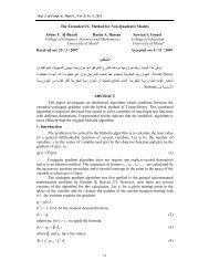
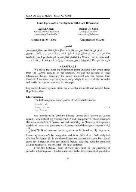
Azad.I.Amen and Rizgar .H. SalihSince σ > β + 1, we can write σ = β + 1+c ,c>0 after substitutingσ = β + 1+ c in eq (31), Maple program tells us a>0 and b0 that the equilibrium point A+at thebifurcation point is unstable. Since ω>0 and b0 according to the Hopf bifurcation theorem, the system (1) hasunstable limit cycle (sub critical Hopf bifurcation). If we take8σ = 10 , β = as example then a = 0.004580131420 and b = -0.053449605993since a>0 system (1) has unstable limit cycle see ,figure (2).From eq(9) because the ρ& is separated,so.ρ =( a +dµdµ) er0( −2dµt )Since the parameters a and d are known from (eq (39),eq (25)) wehave an up to third order approximate expression for the radius of the limitcycle and the dynamics with which the limit cycle will be reacheddepending on the parameter µ.(a)94

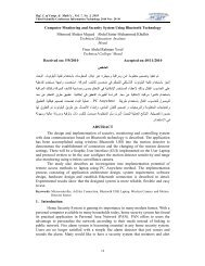
Limit Cycles of Lorenz …(b)Figure (1): Equilibrium bifurcation diagrams of Lorenz system dependenceon r of: (a) x,y; (b) z. The solid curves depict stable behavior and the dotedcurves depict unstable behaviorFigure(2.a)phase portraite for system(1)when 8σ = 10 , β = andr = 22395

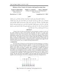
Azad.I.Amen and Rizgar .H. SalihFigure (2.b): phase portrait for system (1)when8 470σ = 10 , β = and r = .3 198Figure (2.c): phase portrait for system (1) when σ = 10 , β = and r = 28.396

Limit Cycles of Lorenz …ConclusionsIn this paper we began to study the Lorenz system. Some insights onstability and bifurcation are obtained. The system posses a Hopf bifurcationand, in particular the case which is analyzed obtained that bifurcation issubcritical (unstable limit cycle) . Analyzing the Hopf bifurcation we showthat the arising unstable limit cycle is near a bifurcation point. It means that,for the Lorenz system, the appearance and location of limit cycles in vicinityat the equilibrium only occurs at very specific values of the parametersdefining the equations.97

Azad.I.Amen and Rizgar .H. SalihREFRENCES[1] Ahmad,.N.M, “The Periodic Solutions for Controlled BiologicalSystems”, Msc .Thesis,College of Siences ,University of Baghdad,(1992).[2] Carr,J., “Application of Center Manifold Theory”, Springer-verlag,New York (1981).[3] Char, B.W., “Maple 7 Learning Guide”, Waterloo maple Inc.,(2001).[4] David,B and Mylan,R “Mathematical Computing An Introductionto Programming Using Maple”, Springer- verlag New York, (2002).[5] Guckenheimer.J and Holmes.P, “Nonlinear oscillations, Dynamicalsystems, and Bifurcations of vector Fields”, Springer, New York,(2002).[6] Lorenz, E.N, “Deterministic Non-Periodic Flow”, J. Atmos. Sci, vol20, (1963) ,130-141.[7] Lynch, S., “Dynamical Systems With Applications Using Maple”,Birkhauser, Boston, (2001).[8] Marsden, J.E and McCracken, M.,”The Hopf Bifurcation and itsApplication”, Springer-verlag.,NY, (1978).[9] Palacian,J. and Yanguas.p, “Periodic Orbits of the Lorenz Systemthrough Perturbation Theory”,.International Journal of Bifurcationand Chaos, vol.11, No.10 (2001), 2559-2566[10] Pushpavanam ,S.,“Mathematical Methods in Chemical Engineering", prentice, Hall private.Limited, New Delhi, (2005).[11] Qian,H., “Deterministic and stochastic Dynamical System”,Springer, (2003)[12] Rao,M.R., “Ordinary Differential Equation”, Affiliated east-westpress , New Delhi-Madras, (1980).[13] Stephen,J.Merrill, “A Model of the Stimulation of B-cells byReplicating Antigen-ΙΙ”.,Mathematical Biosciences, 41: (1978) 143-155.[14] Sparrow, C. “The Lorenz Equation, Bifurcation, Chaos and StrangeAttractors”, Springer- Verlag ,New York, (1982).[15] Teschl,G., “Ordinary Differential Equation and DynamicalSystems”, typeset by Ams-latex and Makeindex,(2004).98

Limit Cycles of Lorenz …[16] Yu,P. “Computation of Normal Form via a Perturbation Technique”Journal of Sound andVibration 211(1), (1988) ,19-38.[17] Yu,P., “Simplest Normal forms of Hopf and Generalized HopfBifurcations”, International Journal of Bifurcation and Chaos, Vol.9,N.10 (1999) 1917-1923.[18] Yu,P. “A matching Pursuit Technique for Computing the SimplestNormal Form of Vecter Field”, Jornal of Symbolic Computation,35, (2003) 591-615.99