a consistent nonparametric test for causality in quantile - Humboldt ...

Econometric Theory, 28, 2012, 861–887.doi:10.1017/S0266466611000685A CONSISTENT NONPARAMETRICTEST FOR CAUSALITY IN QUANTILEKIHO JEONGKyungpook National UniversityWOLFGANG K. HÄRDLEHumboldt-Universität zu BerlinSONG SONGHumboldt-Universität zu BerlinandUniversity of California, BerkeleyThis paper proposes a nonparametric test of Granger causality in quantile. Zheng(1998, Econometric Theory 14, 123–138) studied the idea to reduce the problemof testing a quantile restriction to a problem of testing a particular type of meanrestriction in independent data. We extend Zheng’s approach to the case of dependentdata, particularly to the test of Granger causality in quantile. Combining the resultsof Zheng (1998) and Fan and Li (1999, Journal of Nonparametric Statistics 10,245–271), we establish the asymptotic normal distribution of the test statistic undera β-mixing process. The test is consistent against all fixed alternatives and detectslocal alternatives approaching the null at proper rates. Simulations are carried outto illustrate the behavior of the test under the null and also the power of the testunder plausible alternatives. An economic application considers the causal relationsbetween the crude oil price, the USD/GBP exchange rate, and the gold price in thegold market.1. INTRODUCTIONWhether movements in one economic variable cause reactions in another variableis an important issue in economic policy and also for financial investmentdecisions. A framework for investigating causality between economic indicatorshas been developed by Granger (1969). Testing for Granger causality betweenThe research was conducted while Jeong was visiting C.A.S.E.—Center for Applied Statistics and Economics—Humboldt-Universität zu Berlin in the summers of 2005 and 2007. Jeong is grateful for their hospitality duringthe visits. Jeong’s work was supported by a Korean Research Foundation grant funded by the Korean government(MOEHRD) (KRF-2006-B00002), and Härdle and Song’s work was supported by the Deutsche Forschungsgemeinschaftthrough the SFB 649 “Economic Risk.” We thank the editor, two anonymous referees, and Holger Dette forconcrete suggestions on improving the manuscript and restructuring the paper. Their valuable comments and suggestionsare gratefully acknowledged. Address correspondence to Kiho Jeong, Kyungpook National University, Korea;e-mail: khjeong@knu.ac.kr.c○ Cambridge University Press 2012 861

862 KIHO JEONG ET AL.economic time series has been since studied intensively in empirical macroeconomicsand empirical finance. The majority of research results were obtained inthe context of Granger causality in the conditional mean. The conditional mean,though, is a questionable element of analysis if the distributions of the variablesinvolved are nonelliptic or fat tailed as is to be expected with, for example, financialreturns. The focus of a causality analysis on the mean might result in unclearnews. The conditional mean is only one element of an overall summary for theconditional distribution. A tail area causal relation may be quite different froma causality based on the center of the distribution. Lee and Yang (2007) exploremoney-income Granger causality in the conditional quantile and find that Grangercausality is significant in tail quantiles, whereas it is not significant in the centerof the distribution.An illustrating motivation for the research presented here is from labor marketanalysis where one tries to find out how income depends on the age of the employeefor different education levels, genders, and nationalities, and so on (discriminationeffects); see, for example, Buchinsky (1995). In particular, the effectof education on income is summarized by the basic claim of Day and Newburger(2007): At most ages, more education equates with higher earnings, and the payoffis most notable at the highest educational level, which is actually from thepoint of view of mean regression. However, whether this difference is significantor not is still questionable, especially for different ends of the (conditional)income distribution. Härdle, Ritov, and Song (2009) show that for the 0.20 quantileconfidence bands for income given “university,” “apprenticeship,” and “loweducation” status do not differ significantly from one another although they becomeprogressively lower, which indicates that high education does not equateto higher earnings significantly for the lower tails of income, whereas increasingage seems to be the main driving force. For the conditional median, the bandsfor “university” and “low education” differ significantly. For the 0.80 quantiles,all conditional quantiles differ, which indicates that higher education is associatedwith higher earnings. However, these findings do not necessarily indicatecausalities. To answer the question “Does education Granger cause income invarious conditional quantiles?” the concept of Granger causality in means cannotbe used to estimate or test for these effects. Hence the need for the conceptof Granger causality in quantiles and the need to develop tests for these effectsemerge.Another motivation comes from controlling and monitoring downside marketrisk and investigating large comovements between financial markets. These areimportant for risk management and portfolio/investment diversification (Hong,Liu, and Wang, 2009). Various other risk management tasks are described inBollerslev (2001) and Campbell and Cochrane (1999) indicating the importanceof Granger causality in quantile. Yet another motivation comes from thewell-known robustness properties of the conditional quantile: like the parallelboxplot—calculated across an explanatory variable—the set of conditionalquantiles characterizes the entire distribution in more detail.

NONPARAMETRIC TEST FOR CAUSALITY IN QUANTILE 863Based on the kernel method, we propose a nonparametric test for Grangercausality in quantile. Testing conditional quantile restrictions by nonparametricestimation techniques in dependent data situations has not been considered in theliterature before. This paper intends to fill this literature gap. In an unpublishedworking paper that has been independently carried out from ours, Lee and Yang(2007) also propose a test for Granger causality in the conditional quantile. Theirtest, however, relies on linear quantile regression and thus is subject to possiblefunctional misspecification of quantile regression. Recently, Hong et al. (2009) investigatedGranger causality in value at risk (VaR) with a corresponding (kernelbased)test. Their method, however, offers two possible improvements. The first isthat it needs a parametric specification of VaR, again subject to misspecificationerrors. The second is that their test does not directly check causality but rather anecessary condition for causality.The problem of testing conditional mean restrictions using nonparametric estimationtechniques has been actively studied for dependent data. Among the relatedwork, the testing procedures of Fan and Li (1999) and Li (1999) use thegeneral hypothesis of the form E(ε|z) = 0, where ε and z are the regression errorterm and the vector of regressors, respectively. They consider the distancemeasure of J = E[εE(ε|z) f (z)] to construct kernel-based procedures. For the advantagesof using this distance measure in kernel-based testing procedures, seeLi and Wang (1998) and Hsiao and Li (2001). A feasible test statistic based onJ has a second-order degenerate U-statistic as the leading term under the nullhypothesis. Generalizing the result of Hall (1984) for independent data, Fan andLi (1999) establish the asymptotic normal distribution for a general second-orderdegenerate U-statistic with dependent data.All the results stated previously on testing mean restrictions are however irrelevantwhen testing quantile restrictions. Zheng (1998) proposed an idea to transformquantile restrictions to mean restrictions in independent data. Following hisidea, one can use the existing technical results on testing mean restrictions in testingquantile restrictions. In this paper, by combining Zheng’s idea and the resultsof Fan and Li (1999) and Li (1999), we derive a test statistic for Granger causalityin quantile and establish the asymptotic normal distribution of the proposedtest statistic under a β-mixing process. Our testing procedure can be extended toseveral hypothesis testing problems with conditional quantile in dependent data;for example, testing a parametric regression functional form, testing the insignificanceof a subset of regressors, and testing semiparametric versus nonparametricregression models.The paper is organized as follows. Section 2 presents the test statistic. Section3 establishes the asymptotic normal distribution under the null hypothesis ofno causality in quantile. Section 4 displays a fairly extensive simulation study toillustrate the behavior of the test under the null, in addition to the power of thetest under plausible alternatives. Section 5 considers the causal relations betweenthe crude oil and gold prices as an economic application. Section 6 concludes thepaper. Technical proofs are given in the Appendix.

864 KIHO JEONG ET AL.2. NONPARAMETRIC TEST FOR GRANGER CAUSALITYIN QUANTILETo simplify the exposition, we assume a bivariate case, or that only {y t ,w t } areobservable. Granger causality in mean (Granger, 1988) is defined as follows.1. w t does not cause y t in mean with respect to {y t−1 ,...,y t−p ,w t−1 ,...,w t−q } ifE( y t |y t−1 ,...,y t−p ,w t−1 ,...,w t−q ) = E( y t |y t−1 ,...,y t−p ) and2. w t is a prima facie cause in mean of y t with respect to {y t−1 ,...,y t−p ,w t−1 , ...,w t−q } ifE( y t |y t−1 ,...,y t−p ,w t−1 ,...,w t−q ) ≠ E( y t |y t−1 ,...,y t−p ).Motivated by the definition of Granger causality in mean, we define Grangercausality in quantile as follows.1. w t does not cause y t in the θ-quantile with respect to {y t−1 ,...,y t−p ,w t−1 ,..., w t−q } ifQ θ ( y t |y t−1 ,...,y t−p ,w t−1 ,...,w t−q ) = Q θ ( y t |y t−1 ,...,y t−p ). (1)2. w t is a prima facie cause in the θ-quantile of y t with respect to {y t−1 ,...,y t−p ,w t−1 ,...,w t−q } ifQ θ ( y t |y t−1 ,...,y t−p ,w t−1 ,...,w t−q ) ≠ Q θ ( y t |y t−1 ,...,y t−p ), (2)where Q θ (y t |·) is the θth (0

NONPARAMETRIC TEST FOR CAUSALITY IN QUANTILE 865Zheng (1998) proposed an idea to reduce the problem of testing a quantile restrictionto a problem of testing a particular type of mean restriction. The null hypothesis(3) is true if and only if E[1{y t Q θ (x t )|z t }] = θ or 1{y t Q θ (x t )} =θ + ε t where E(ε t |z t ) = 0 and 1(·) is the indicator function. For a list of relatedliterature we refer to Li and Wang (1998) and Zheng (1998). Although variousdistance measures can be used to consistently test the hypothesis (3), we considerthe following distance measure:{Fy|zJ ≡ E[(Q θ (x t )|z t ) − θ } ]2 fz (z t ) , (5)with f zt (z t ) being the marginal density function of z t , which is sometimes abbreviatedas f z (z t ). Note that J 0 and the equality holds if, and only if, H 0 istrue, with strict inequality holding under H 1 . Thus J can be used as a propercandidate for consistent testing of H 0 (Li, 1999, p. 104). Because E(ε t |z t ) =F y|z {Q θ (x t )|z t } − θ we haveJ = E{ε t E(ε t |z t ) f z (z t )}. (6)The test is based on a sample analogue of E{ε E(ε|z) f z (z)}. Including the densityfunction f z (z) avoids the problem of trimming on the boundary of the densityfunction; see Powell, Stock, and Stoker (1989) for an analogue approach. Thedensity-weighted conditional expectation E(ε|z) f z (z) can be estimated by kernelmethodsÊ(ε t |z t ) ˆ f z (z t ) =1T(T − 1)h ∑ m K ts ε s , (7)s≠twhere m = p + q is the dimension of z, K ts = K {(z t − z s )/h} is the kernelfunction, and h is a bandwidth. Then we have a sample analogue of J asJ T ≡=1T (T − 1)h m1T (T − 1)h mT T∑ ∑t=1 s≠tT T∑ ∑t=1 s≠tK ts ε t ε sK ts [1{y t Q θ (x t )} − θ][1{y s Q θ (x s )} − θ]. (8)The θth conditional quantile of y t given x t , Q θ (x t ), can also be estimated by thenonparametric kernel methodˆQ θ (x t ) = ˆF y|x −1 (θ|x t), (9)where∑ L ts 1(y s y t )s≠tˆF y|x (y t |x t ) =(10)∑ L tss≠tis the Nadaraya–Watson kernel estimator of F y|x (y t |x t ) with the kernel functionof L ts = L (x t − x s )/a and the bandwidth parameter of α. The unknown error εcan be estimated as

NONPARAMETRIC TEST FOR CAUSALITY IN QUANTILE 867(e) For any y and x satisfying 0 < F y|x (y|x) 0, F y|x andf x (x) are continuous and bounded in x and y; for fixed y, the conditionaldistribution function F y|x and the conditional density function f y|x belongto A ∞ 3 ; f y|x(Q θ (x)|x)>0 for all x; f y|x is uniformly bounded in x and yby, say, c f .(f) For some compact set G, there are ε>0 and γ>0 such that f x γfor all x in the ε-neighborhood {x|‖x − u‖ 0,f y|x (y|x) c 0 for all x ∈ G,v ∈ .(g) There is an increasing sequence s T of positive integers such that for somefinite A,(A2)Ts Tβ 2s T /(3T ) (s T ) A, 1 s T T 2for all T 1.(a) We use product kernels for both L (·) and K (·). Let l and k be their correspondingunivariate kernel which is bounded and symmetric. Then l(·) isnonnegative, l(·) ∈ ϒ v , k(·) is nonnegative, and k(·) ∈ ϒ 2 .(b) h = O(T −α′ ) for some 0 0, sup y∈φzρ∣ ∣ g(y) − g(z) − G g (y, z) ∣ ∣ /|y − z| μ D g (z) for all z,where φ zρ = {y||y − z|

868 KIHO JEONG ET AL.homogeneous polynomial in y − z with coefficients being the partial derivativesof g at z of orders 1 through d − 1 when d > 1; and g(z), its partial derivativesof order d − 1 and less, and D g (z) have finite αth moments.The functions in A α μ are thus expanded in a Taylor series with a local Lipschitzcondition on the remainder, (α,μ) depending simultaneously on smoothness andmoment properties. Bounded functions in Lip(μ) (the Lipschitz class of degree μ)for 0 1, Aα μ contains the bounded and (d − 1)-timesboundedly differentiable functions whose (d − 1)th partial derivatives are in Lip(μ − d + 1)). In applying A α μ to f and F, we take α =∞.Conditions (A1)(a)–(d) and (A2)(a) and (b) are adopted from conditions (D1)and (D2) of Li (1999), which are used to derive the asymptotic normal distributionof a second-order degenerate U-statistic. Assumption (A1)(a) requires {y t ,w t }t=1Tto be a stationary absolutely regular process with geometric decay rate. Assumptions(A1)(b)–(d) are mainly some smoothness and moment conditions; these conditionsare quite weak in the sense that they are similar to those used in Fan andLi (1996) for the independent data case. However, for autoregressive conditionallyskedastic (ARCH) or generalized autoregressive conditionally heteroskedastic(GARCH) type error processes as considered in Engle (1982) and Bollerslev(1986), the error term ε t may not have finite fourth moments in some situations.For example, let ε t |ε t−1 ∼ N(0,α 0 + α 1 εt−1 2 ). Engle (1982) showed that ε t doesnot have a finite fourth moment if α 1 > 1/ √ 3. Thus, Assumption (A1)(c) will beviolated in such a case.Assumption (A2)(a) requires L(·) to be a vth- (v 2 ) order kernel. This conditiontogether with (A1)(b) ensures that the bias in the kernel estimation (of thenull model) is bounded. The requirement that k is a nonnegative second-orderkernel function in (A2)(b) is a quite weak and standard assumption.Conditions (A1)(e)–(g) and (A2)(c) are technical conditions (A1), (A2), (B1),(B2), (C1), and (C2) of Theorem 2.3 of Franke and Mwita (2003), which are requiredto get the uniform convergence rate of the nonparametric kernel estimatorof the conditional distribution function and corresponding conditional quantilewith mixing data. Because the simple ARCH models (Engle, 1982; Masry andTjøstheim, 1995, 1997), their extensions (Diebolt and Guegan, 1993), and thebilinear Markovian models are geometrically strongly mixing under some generalergodicity conditions, Assumption (A1)(g) is usually satisfied. There also existsimple methods to determine the mixing rates for various classes of random processes,for example, Gaussian, Markov, autoregressive moving average, ARCH,and GARCH. Hence the assumption of a known mixing rate is reasonable andhas been adopted in many studies, for example, Györfi, Härdle, Sarda, and Vieu(1989), Irle (1997), Meir (2000), Modha and Masry (1998), Roussas (1988), andYu (1993). Auestad and Tjøstheim (1990) provided excellent discussions on therole of mixing for model identification in nonlinear time series analysis. But sincethe restriction of Assumption (A1)(c) as discussed before, ARCH or GARCHtype processes may not satisfy all assumptions here. Finally conditions (A2)(d)

870 KIHO JEONG ET AL.Th m/2 Ĵ T / ˆσ 0√T=T − 1T∑t=1T∑s≠t(iii) Under the alternative hypothesis (4),{ } ][ {} ]K ts[1 y t ˆQ θ (x t ) − θ 1 y s ˆQ θ (x s ) − θ√ √2θ(1 − θ) ∑ Kts2s≠t.Ĵ T → E{[F y|z (Q θ (x t )|z t ) − θ] 2 f z (z t )} > 0in probability.(iv) Under the local alternatives (A.2) in the Appendix, T h m/2 Ĵ T → N(μ,σ1 2)in distribution, where[]μ = E fy|z 2 {Q θ (z t )|z t }l 2 (z t ) f z (z t ) ,}∫σ1 {σ 2 = 2E v 4 (z t) f z (z t ) K 2 (u)du, andσ 2 v (z t) = E(v 2 t |z t) with v t ≡ I {y t Q θ (x t )} − F(Q θ (x t )|z t ).Theorem 3.1 generalizes the results of Zheng (1998) for independent data tothe weakly dependent data case. A detailed proof of Theorem 3.1 is given inthe Appendix. The main difficulty in deriving the asymptotic distribution of thestatistic defined in equation (12) is that a nonparametric quantile estimator isincluded in the indicator function that is not differentiable with respect to thequantile argument and thus prevents taking a Taylor expansion around the trueconditional quantile Q θ (x t ). To circumvent the problem, Zheng (1998) madeuse of the work of Sherman (1994) on uniform convergence of U-statistics indexedby parameters. In this paper, we bound the test statistic by the statisticsin which the nonparametric quantile estimator in the indicator function is replacedwith sums of the true conditional quantile and upper and lower boundsconsistent with the uniform convergence rate of the nonparametric quantile estimator,1(y t Q θ (x t ) − C T ) and 1(y t Q θ (x t ) + C T ).An important further step is to show that the differences of the ideal test statisticJ T given in equation (8) and the statistics having the indicator functions obtainedfrom the first step stated previously are asymptotically negligible. We may directlyshow that the second moments of the differences are asymptotically negligible byusing the result of Yoshihara (1976) on the bound of moments of U-statisticsfor absolutely regular processes. However, it is tedious to get bounds on thesecond moments with dependent data. In the proof we use instead the fact thatthe differences are second-order degenerate U-statistics. Thus by using the resulton the asymptotic normal distribution of the second-order degenerate U-statisticof Fan and Li (1999), we can derive the asymptotic variance that is based on theindependent and identically distributed (i.i.d.) sequence having the same marginaldistributions as weakly dependent variables in the test statistic. With this little

NONPARAMETRIC TEST FOR CAUSALITY IN QUANTILE 871trick we only need to show that the asymptotic variance is O(1) in an i.i.d.situation. For details refer to the Appendix.4. SIMULATIONWe generate bivariate data {y t ,w t } t=1 T according to the following model:y t = 1 2 y t−1 + cw 2 t−1 + ε 1t,w t = 1 + 1 2 w t−1 + ε 2t ,where ε 1t and ε 2t are independent standard normal random variables. Here c = 0corresponds to the hypothetical model; that is, w t does not cause y t in the θquantile with respect to {y t−1 ,w t−1 }. All the coefficients are set such that thecorresponding time series is stationary and β-mixing with corresponding densitiesbounded to satisfy the assumptions discussed before. We use different values ofc ∈ [0,1] to investigate the power of the test, such that the higher c is, the strongerthe causality of w t on y t is. Without loss of generality, we choose θ = 0.1,0.5,0.9and T = 500,1,000,5,000 here with the bandwidth h and a as in (7) and (10)as for a typical Nadaraya–Watson type estimator. We consider the nominal 0.05significance level and repeat the test 500 times to generate the power.Table 1 displays the power performance of the test for different combinationsof T, c, and θ. First, obviously the power is very sensitive to the choice of T ; thatis, the larger T is, for the same c and θ, the larger the power is. From a technicalpoint of view, this makes sense, because the more data we have, the more evidencewe can draw from to detect the “causality” effect. Our asymptotic result, Theorem3.1, needs the plug-in estimation of the asymptotic covariance matrix that is usedto normalize the test statistic. Note that such an estimator is model-dependent andunder the alternative is consistent with a different value than the one under thenull. As a result, the power deteriorates for small T . On the other hand, whetherthe causality effect exists or not is the nature of the series, which is independent ofthe sample size used in this technical test. Enhancing the power performance forsmall-sample data using the simulation-based method deserves further research.Second, as discussed before, the higher c is, the stronger the causality of w t on y tis, which is confirmed by the larger and larger power values. Third, for differentquantiles θ, we find that the powers with respect to θ = 0.5 are usually larger thanthe powers with respect to θ = 0.1 and 0.9.5. APPLICATION TO COMMODITY PRICESIn financial and commodity markets, it has been argued that the covariation ofthe tails may be different from that of the rest of the distribution. The gold marketis one of the most important markets in the world, where trading takes place24 hours a day around the globe and transactions involving billions of dollars of

872 KIHO JEONG ET AL.TABLE 1. Power performance for different combinations of T,c, and θc Power (θ 0.1) c Power (θ 0.5) c Power (θ 0.9)T = 5000.00 0.024 0.00 0.108 0.00 0.0100.03 0.030 0.03 0.288 0.03 0.0200.06 0.058 0.06 0.796 0.06 0.1080.09 0.190 0.09 0.991 0.09 0.5850.12 0.414 0.12 1.000 0.12 0.9500.15 0.696 0.15 1.000 0.15 0.9940.18 0.888 0.18 1.000 0.18 1.0000.21 0.962 0.21 1.000 0.21 1.0000.24 0.988 0.24 1.000 0.24 1.0000.27 1.000 0.27 1.000 0.27 1.0000.30 1.000 0.30 1.000 0.30 1.000T = 1,0000.00 0.014 0.00 0.130 0.00 0.0180.01 0.022 0.01 0.144 0.01 0.0240.02 0.038 0.02 0.296 0.02 0.0240.03 0.026 0.03 0.564 0.03 0.0400.04 0.060 0.04 0.788 0.04 0.1080.05 0.110 0.05 0.946 0.05 0.2840.06 0.196 0.06 0.990 0.06 0.5060.07 0.356 0.07 1.000 0.07 0.8380.08 0.530 0.08 1.000 0.08 0.9500.09 0.676 0.09 1.000 0.09 0.9940.10 0.816 0.10 1.000 0.10 0.9960.11 0.906 0.11 1.000 0.11 1.0000.12 0.958 0.12 1.000 0.12 1.0000.13 0.972 0.13 1.000 0.13 1.0000.14 0.994 0.14 1.000 0.14 1.0000.15 0.998 0.15 1.000 0.15 1.0000.16 1.000 0.16 1.000 0.16 1.000T = 5,0000.00 0.020 0.00 0.116 0.00 0.0260.01 0.028 0.01 0.328 0.01 0.0460.02 0.124 0.02 0.904 0.02 0.1420.03 0.490 0.03 1.000 0.03 0.7280.04 0.924 0.04 1.000 0.04 0.9880.05 1.000 0.05 1.000 0.05 1.0000.06 1.000 0.06 1.000 0.06 1.0000.07 1.000 0.07 1.000 0.07 1.0000.08 1.000 0.08 1.000 0.08 1.0000.09 1.000 0.09 1.000 0.09 1.0000.10 1.000 0.10 1.000 0.10 1.000

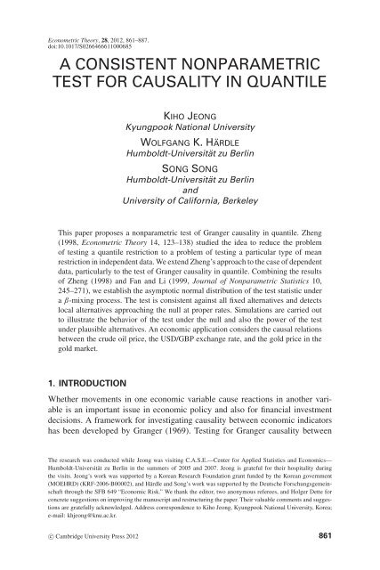
NONPARAMETRIC TEST FOR CAUSALITY IN QUANTILE 873TABLE 2. Unit root testsTime CR Unit rootTest trend Test value Unit afterVariable type term statistics 5% root differencingLN Oil DF no 0.86955 −1.94160 yes noADF no 0.72255 −1.94160 yes noPP no 0.73107 −1.94160 yes noKPSS no 2.16221 0.14600 yes noDF include −0.81819 −2.86386 yes noADF include −1.03287 −2.86386 yes noPP include −0.94355 −2.86386 yes noKPSS include 2.16221 0.14600 yes noGBP DF no −0.12461 −1.94160 yes noADF no −0.16186 −1.94160 yes noPP no −0.12506 −1.94160 yes noKPSS no 5.26720 0.14600 yes noDF include −1.53295 −2.86386 yes noADF include −1.51000 −2.86386 yes noPP include −1.53853 −2.86386 yes noKPSS include 5.26720 0.14600 yes noLN Gold DF no 0.45931 −1.94160 yes noADF no 1.03139 −1.94160 yes noPP no 0.69975 −1.94160 yes noKPSS no 3.50910 0.14600 yes noDF include −1.98422 −2.86386 yes noADF include −1.36627 −2.86386 yes noPP include −1.66336 −2.86386 yes noKPSS include 3.50910 0.14600 yes noNote: ”LN Oil”, ”GBP”, and ”LN Gold” refer to the logarithmic Brent crude oil price, USD/GBP exchange rate, andlogarithmic NYMEX spot gold price, respectively. The “Test types” DF, ADF, PP, and KPSS refer to unit root testsof, respectively, Dickey–Fuller (Fuller, 1976), augmented Dickey–Fuller (Fuller, 1976), Phillips–Perron (Phillips &Perron, 1988), and (Kwaitkowski et al., 1992).gold are carried out each day. Understanding the mechanism of gold price changesis important for many outstanding issues in international economics and finance.Market participants are increasingly concerned with their exposure to large goldprice fluctuations with special interest in which factors drive the changes. In thissection, we apply the quantile causality test to investigate relations between theBrent crude oil, USD/GBP exchange rate and NYMEX spot gold prices (in USDper barrel and per ounce, respectively). The data, as seen in Figure 1, obtainedfrom Datastream, are daily observations from 20 February 1997 to 17 July 2009(T = 3,237). We use the USD/GBP instead of USD/EUR because the euro wasonly introduced as a new currency from 1 January 1999. As indicated by Table 2,we assume differenced logarithmic data are stationary and β-mixing with correspondingdensities bounded. Because a long memory effect is not expected, wechoose p = q = 1 and m = 2.

874 KIHO JEONG ET AL.FIGURE 1. Plot of the gold prices, oil price, and exchange rate time series from 20February 1997 to 17 July 2009.FIGURE 2. Test statistics with respect to different quantiles for the oil-gold prices causalitytest.Figures 2 and 3 present results of testing whether oil prices Granger cause goldprices and whether the USD/GBP exchange rate Granger causes gold prices atthe various quantiles, respectively, where logarithmic returns instead of the rawobservations are used. The solid line and dotted line represent the standardizedtest statistics with respect to different quantiles (x-axis) and the critical value1.96, respectively. In Figures 2 and 3, because the test statistic exceeds the criticalvalue when 0.22 ≤ θ ≤ 0.80, we conclude that the oil price and exchange ratechanges do not cause the gold price change in θ0.80, whereas it isa prima facie cause in the 0.22 ≤ θ ≤ 0.80 quantile, respectively. For example, theoil price and USD/GBP exchange rate increases suggest that investors are wary ofthe U.S. dollar’s weakness and inflation. Because gold is typically bought as an

NONPARAMETRIC TEST FOR CAUSALITY IN QUANTILE 875FIGURE 3. Test statistics with respect to different quantiles for the exchange rate-goldprices causality test.alternative to the dollar among safe-haven assets, investors seeking safety frominflation risk and currency devaluation will cause the gold price to rise. However,the extreme low and high changes of the gold market may be caused by speculation.This is consistent with most of the empirical findings in the literature that thecodependency may be stronger in the center than in the tails. By combining resultsfrom Figures 2 and 3, we find that the oil price and exchange rate changes have asignificant predictive power for nonextreme gold price changes, which is, however,not significant for extreme changes. This finding could help to make it possible touse the gold price and GBP to hedge oil price changes in a more precise way withmore careful investigation of their relations, which deserves further research.6. CONCLUSIONBy extending the Zheng (1998) idea to dependent data, we propose a consistenttest for Granger causality in conditional quantile. The appealing feature of ourproposed test is that it can investigate Granger causality in various conditionalquantiles. The benefit of this is illustrated in the commodity market applicationwhere the causal relationships among the oil price, USD/GBP exchange rate, andgold price were shown to be different between a tail area and in the center of thedistribution. We also illustrate that oil price and USD/GBP changes have significantpredictive power on nonextreme gold price changes.The test can be extended in a number of ways to test conditional quantile restrictionswith dependent data: First, it can be extended to test functional misspecification,or the insignificance of a subset of regressors in quantile regressionfunction, and second, it can also be used to test some semiparametric versus nonparametricmodels in quantile regression models.

876 KIHO JEONG ET AL.REFERENCESAuestad, B. & D. Tjøstheim (1990) Identification of nonlinear time series: First order characterisationand order determination. Biometrica 77, 669–687.Bollerslev, T. (1986) Generalized autoregressive conditional heteroskedasticity. Journal of Econometrics31, 307–327.Bollerslev, T. (2001) Financial econometrics: Past developments and future challenges. Journal ofEconometrics 100, 41–51.Buchinsky, M. (1995) Quantile regression, Box-Cox transformation model, and the U.S. wage structure.1963–1987. Journal of Econometrics 65, 65–154.Campbell, J. & J. Cochrane (1999) By force of habit: A consumption-based explanation of aggregatestock market behaviour. Journal of Political Economy 107, 205–251.Day, J.C. & E.C. Newburger (2002) The big payoff: Educational attainment and synthetic estimatesof work-life earnings. Special studies. Current population reports. Statistical report p23–210, U.S.Department of Commerce, U.S. Census Bureau.Diebolt, J. & D. Guégan (1993) Tail behavior of the stationary density of general nonlinear autoregressiveprocesses of order 1. Journal of Applied Probability 30, 315–329.Engle, R. (1982) Autoregressive conditional heteroskedasticity with estimates of the variance ofUnited Kingdom inflation. Econometrica 50, 987–1007.Fan, Y. & Q. Li (1996) Consistent model specification tests: Omitted variables, parametric and semiparametricfunctional forms. Econometrica 64, 865–890.Fan, Y. & Q. Li (1999) Central limit theorem for degenerate U-statistics of absolutely regular processeswith applications to model specification tests. Journal of Nonparametric Statistics 10,245–271.Franke, J. & P. Mwita (2003) Nonparametric Estimates for Conditional Quantiles of Time Series.Wirtschaftsmathematik 87, University of Kaiserslautern.Fuller, W. (1976) Introduction to Statistical Time Series. Wiley.Granger, C. (1969) Investigating causal relations by econometric models and cross-spectral methods.Econometrica 37, 424–438.Granger, C. (1988) Some recent developments in a concept of causality. Journal of Econometrics 39,199–211.Györfi, L., W. Härdle, P. Sarda, & P. Vieu (1989) Nonparametric Curve Estimation from Time Series.Springer-Verlag.Hall, P. (1984) Central limit theorem for integrated square error of multivariate nonparametric densityestimators. Journal of Multivariate Analysis 14, 1–16.Härdle, W., Y. Ritov, & S. Song (2009) Bootstrap Partial Linear Quantile Regression and ConfidenceBands. SFB649 Discussion paper 2010-002, Humboldt Universität zu Berlin.Härdle, W. & T. Stoker (1989) Investigating smooth multiple regression by the method of averagederivatives. Journal of the American Statistical Association 84, 986–995.Hong, Y., Y. Liu, & S. Wang (2009) Granger causality in risk and detection of extreme risk spilloverbetween financial markets. Journal of Econometrics 150, 271–287.Hsiao, C. & Q. Li (2001) A consistent test for conditional heteroskedasticity in time-series regressionmodels. Econometric Theory 17, 188–221.Irle, A. (1997) On the consistency in nonparametric estimation under mixing assumptions. MultivariateAnalysis 60, 123–147.Kwiatkowski, D., P.C.B. Phillips, P. Schmidt, & Y. Shin (1992) Testing the null hypothesis ofstationarity against the alternative of a unit root. Journal of Econometrics 54, 159–178.Lee, T. & W. Yang (2007) Money-Income Granger-Causality in Quantiles. Manuscript, University ofCalifornia, Riverside.Li, Q. (1999) Consistent model specification tests for time series econometric models. Journal ofEconometrics 92, 101–147.Li, Q. & S. Wang (1998) A simple consistent bootstrap test for a parametric regression functionalform. Journal of Econometrics 87, 145–165.

NONPARAMETRIC TEST FOR CAUSALITY IN QUANTILE 877Masry, E. & D. Tjøstheim (1995) Nonparametric estimation and identification of nonlinear ARCHtime series: Strong convergence and asymptotic normality. Econometric Theory 11, 258–289.Masry, E. & D. Tjøstheim (1997) Additive nonlinear ARX time series and projection estimates.Econometric Theory 13, 214–252.Meir, R. (2000) Nonparametric time series prediction through adaptive model selection. MachineLearning 39, 5–34.Modha, D. & E. Masry (1998) Memory-universal prediction of stationary random processes. IEEETransactions on Information Theory 44, 117–133.Phillips, P.C.B. & P. Perron (1988) Testing for a unit root in time series regression. Biometricka 75,335–346.Powell, J., J. Stock, & T. Stoker (1989) Semiparametric estimation of index coefficients. Econometrica57, 1403–1430.Robinson, P.M. (1988) Root-n-consistent semiparametric regression. Econometrica 56, 931–954.Roussas, G.G. (1988) Nonparametric estimation in mixing sequences of random variables. Journal ofStatistical Planning and Inference 18, 135–149.Sherman, R. (1994) Maximal inequalities for degenerate U-processes with applications to optimizationestimators. Annals of Statistics 22, 439–459.Yoshihara, K. (1976) Limiting behavior of u-statistics for stationary absolutely regular processes.Zeitschrift für Wahrscheinlichkeitstheorie und Verwandte Gebiete 35, 237–252.Yu, B. (1993) Density estimation in the l1 norm for dependent data with applications. Annals ofStatistics 21, 711–735.Zheng, J. (1998) A consistent nonparametric test of parametric regression models under conditionalquantile restrictions. Econometric Theory 14, 123–138.APPENDIXProof of Theorem 3.1(i). In the proof, we use several approximations to Ĵ T . We definethem now and recall a few already defined statistics for convenience of reference.Ĵ T ≡J T ≡J TU ≡1T (T − 1)h m1T (T − 1)h m1T (T − 1)h mT T∑ ∑ K tsˆε t ˆε s ,t=1 s≠tT T∑ ∑ K ts ε t ε s ,t=1 s≠tT T∑ ∑ K ts ε tU ε sU ,t=1 s≠t1 T TJ TL ≡T (T − 1)h ∑ m ∑ K ts ε tL ε sL ,t=1 s≠t{}where ˆε t = I y t ˆQ θ (x t ) − θ,ε t = I {y t Q θ (x t )} − θ,ε tU = I {y t + C T Q θ (x t )} − θ,ε tL = I {y t − C T Q θ (x t )} − θ,(A.1)(A.2)(A.3)(A.4)and C T is an upper bound consistent with the uniform convergence rate of the nonparametricestimator of conditional quantile given in equation (13). The proof of Theorem 3.1(i)consists of three steps.

878 KIHO JEONG ET AL.Step 1. Asymptotic normality.Th m/2 J T → N(0,σ 2 0 ),(A.5)where σ0 {θ 2 = 2E 2 (1 − θ) 2 ∫ }f (z t )}{K 2 (u)du under the null.Step 2. Conditional asymptotic equivalence. Suppose that both Th m/2 (J T − J TU ) =O p (1) and Th m/2 (J T − J TL ) = O p (1).Then Th m/2 (Ĵ T − J T ) = O p (1). (A.6)Step 3. Asymptotic equivalence.Th m/2 (J T − J TU ) = O p (1) and Th m/2 (J T − J TL ) = O p (1). (A.7)The combination of steps 1–3 yields Theorem 3.1(i).Proof of Step 1. Because J T is a degenerate U-statistic of order 2, the result followsfrom Lemma 3.2.Proof of Step 2. The proof of step 2 is motivated by the technique of Härdle and Stoker(1989) that was used in treating trimming an indicator function asymptotically. Supposethat the following two statements hold:Th m/2 (J T − J TU ) = O p (1) and (A.8)Th m/2 (J T − J TL ) = O p (1).(A.9)Use C T to denote an upper bound consistent with the uniform convergence rate of thenonparametric estimator of conditional quantile given in equation (13). Suppose thatsup| ˆQ θ (x) − Q θ (x)| C T .(A.10)If inequality (A.10) holds, then the following statements also hold:{Q θ (x)>y t + C T }⊂{ˆQ θ (x)>y t }⊂{Q θ (x)>y t − C T }, (A.11)1(Q θ (x)>y t + C T ) 1( ˆQ θ (x)>y t ) 1( Q θ (x)>y t − C T ), (A.12)J TU Ĵ T J TL ,(A.13)|Th m/2 (J T − Ĵ T )| max{|Th m/2 (J T − J TU )|,|Th m/2 (J T − J TL )|}. (A.14)Using (A.10) and (A.14), we have the following inequality:{P |Th m/2 (J T − Ĵ T )| >δ| sup∣ ˆQ}θ (x) − Q θ (x)| C T{} P max{|Th m/2 (J T − J TU )|,|Th m/2 (J T − J TL )|} >δ∣ sup| ˆQ θ (x) − Q θ (x)| C Tfor allδ >0.(A.15)

NONPARAMETRIC TEST FOR CAUSALITY IN QUANTILE 879Invoking Lemma 3.1 and condition (A2)(c), we have}P{sup| ˆQ θ (x) − Q θ (x)| C T → 1 as T →∞. (A.16)By (A.8) and (A.9), as T →∞,wehave{}P max{|Th m/2 (J T − J TU )|,|Th m/2 (J T − J TL )|} >δ → 0 for all δ>0. (A.17)Therefore, as T →∞,}the right-hand side of the inequality (A.15) × P{sup| ˆQ θ (x) − Q θ (x)| C T → 0;}the left-hand side of the inequality (A.15) × P{sup| ˆQ θ (x) − Q θ (x)| C T{}= P |Th m/2 (J T − Ĵ T )| >δ → 0.In summary, we have that if both Th m/2 (J T − J TU ) = O p (1) and Th m/2 (J T − J TL ) =O p (1), then Th m/2 (Ĵ T − J T ) = O p (1).Proof of Step 3. In the remaining proof, we focus on showing that Th m/2 (J T − J TU ) =O p (1), with the proof of Th m/2 (J T − J TL ) = O p (1) being treated similarly. The proofof step 3 is close in line with the proof in Zheng (1998). DenoteH T (s,t, g) ≡ K ts {1(y t g(x t )) − θ}{1(y s g(x s )) − θ} and (A.18)J[g] ≡1T (T − 1)h mT T∑ ∑ H T (s,t, g).t=1 s≠t(A.19)Then we have J T ≡ J[Q θ ] and J TU ≡ J[Q θ −C T ]. We decompose H T (s,t, g) into threeparts:H T (s,t, g) = K ts {1(y t g(x t )) − F(g(x t )|z t )}{1(y s g(x s )) − F(g(x s )|z s )}+2 × K ts {1(y t g(x t )) − F(g(x t )|z t )}{F(g(x s )|z s ) − θ}+ K ts {F(g(x t )|z t ) − θ}{F(g(x s )|z s ) − θ}= H 1T (s,t, g) + 2H 2T (s,t, g) + H 3T (s,t, g). (A.20)Then let J j [g] = 1/(T (T − 1)h m ) ∑T T∑ H jT (s,t, g), i = 1,2,3. We will treat J j [Q θ ] −t=1 s≠tJ j [Q θ − C T ] for j = 1,2,3 separately.(1) Th m/2 [ J 1 (Q θ ) − J 1 (Q θ − C T ) ] = O p (1). By simple manipulation, we haveJ 1 (Q θ ) − J 1 (Q θ − C T )1 T T [=T (T − 1)h ∑ m ∑ H1T (s,t, Q θ ) − H 1T (s,t, Q θ − C T ) ]t=1 s≠t=1T (T − 1)h mT T∑ ∑ K ts{[1(y t Q θ (x t )) − F(Q θ (x t )|z t )]t=1 s≠t×[1(y s Q θ (x s )) − F(Q θ (x s )|z s )]

880 KIHO JEONG ET AL.−[1(y t (Q θ (x t ) − C T )) − F((Q θ (x t ) − C T )|z t )]}×[1(y s (Q θ (x s ) − C T )) − F((Q θ (x s ) − C T )|z s )] .(A.21)To avoid tedious work to get bounds on the second moment of J 1 (Q θ ) − J 1 (Q θ − C T )with dependent data, we note that the right-hand side of (A.21) is a degenerate U-statisticof order 2. Thus we can apply Lemma 3.2 and haveTh m/2 [ J 1 (Q θ ) − J 1 (Q θ − C T ) ] → N(0,σ2 2 ) in distribution, (A.22)where the definition of the asymptotic variance σ2 2 is based on the i.i.d. sequence havingthe same marginal distributions as weakly dependent variables in (A.21). That is,σ 2 2 = 2h−m Ẽ [ H 1T (s,t, Q θ ) − H 1T (s,t, Q θ − C T ) ] 2 ,where the notation Ẽ is an expectation evaluated at an i.i.d. sequence having the samemarginal distribution as the mixing sequences in (A.21) (Fan and Li, 1999, p. 248). Now,to show that Th m/2 [ J 1 (Q θ ) − J 1 (Q θ − C T ) ] = O p (1), we only need to show that theasymptotic variance σ 2 2 (z) is O(1) with i.i.d. data. Use T to denote an upper boundconsistent with the integral over K ts being of the order O(h m ).WehaveẼ [ H 1T (s,t, Q θ ) − H 1T (s,t, Q θ − C T ) ] 2 T Ẽ{[1 t (Q θ ) − F t (Q θ )][1 s (Q θ ) − F s (Q θ )]− [1 t (Q θ − C T ) − F t (Q θ − C T )][1 s (Q θ − C T ) − F s (Q θ − C T )]} 2 T Ẽ{F t (Q θ )[1 − F t (Q θ )] F s (Q θ )[1 − F s (Q θ )]}+ Ẽ{F t (Q θ − C T )[1 − F t (Q θ − C T )] F s (Q θ − C T )[1 − F s (Q θ − C T )]}− 2E{[F t (min(Q θ , Q θ − C T )) − F t (Q θ )F t (Q θ − C T )]× [F s (min(Q θ , Q θ − C T )) − F s (Q θ )F s (Q θ − C T )]}= T Ẽ{[F t (Q θ ) − F t (Q θ )F t (Q θ )][F s (Q θ ) − F s (Q θ )F s (Q θ )]}− T Ẽ{[F t (min(Q θ , Q θ − C T )) − F t (Q θ )F t (Q θ − C T )]× [F s (min(Q θ , Q θ − C T )) − F s (Q θ )F s (Q θ − C T )]}+ T Ẽ{[F t (Q θ − C T ) − F t (Q θ − C T )F t (Q θ − C T )]× [F s (Q θ − C T ) − F s (Q θ − C T )F s (Q θ − C T )]}− T Ẽ{[F t (min(Q θ , Q θ − C T )) − F t (Q θ )F t (Q θ − C T )]× [F s (min(Q θ , Q θ − C T )) − F s (Q θ )F s (Q θ − C T )]} T C T .(A.23)Thus we have that σ 2 2 = O(C T ) = O(1), and soTh m/2 [ J 1 (Q θ ) − J 1 (Q θ − C T ) ] = Op(1).(A.24)

NONPARAMETRIC TEST FOR CAUSALITY IN QUANTILE 881(2) Th m/2 [ J 2 (Q θ ) − J 2 (Q θ − C T ) ] = Op(1). Note that H 2T (s,t, Q θ ) = 0 because ofF y|z (Q θ (x s )|z s ) − θ = 0. Then we haveJ 2 (Q θ ) − J 2 (Q θ − C T ) =−J 2 (Q θ − C T )1 T T ( )1 zt=−T (T − 1)∑ ∑t=1 s≠t h m K − z sh×{1(y t Q θ (x t ) − C T ) − F y|z (Q θ (x t ) − C T |z t )}×{F y|z (Q θ (x s ) − C T |z s ) − θ}.(A.25)By taking a Taylor expansion of F y|z (Q θ (x s ) − C T |z s ) around Q θ (x s ), it equals1 T T ( )1 zt−T (T − 1)∑ ∑t=1 s≠t h m K − z sh×{1(y t Q θ (x t ) − C T ) − F y|z (Q θ (x t ) − C T |z t )}× (−C T ) f y|z ( ¯Q θ (x s )|z s ), (A.26)where ¯Q θ is between Q θ and Q θ − C T . Thus we have(J 2 (Q θ ) − J 2 (Q θ − C T )) 2[1 T T ( )1 ztT (T − 1)∑ ∑t=1 s≠t h m K − z sh× { 1(y t Q θ (x t ) − C T ) − F y|z (Q θ (x t ) − C T |z t ) }] 2 2 C 2 T= 2 C 2 T≡ 2 C 2 T[1 T {T∑ 1(yt Q θ (x t ) − C T ) − F y|z (Q θ (x t ) − C T ) } ] 2fˆz (z t )t=1{}1 T2T∑ u t fˆz (z t )t=1= 2 CT 2 T −2 ∑T u 2 tt=1≡ J 21 + J 22 ,fˆz 2 (z t ) + 2 CT 2 T −2 ∑Tt=1T∑s≠twhere the inequality holds because of Assumption (A.1)(e).E|J 21 | = 2 CT [T 2 T −1 −1 ∑T { } ]E u 2 ˆt fz 2 (z t )t=1(= O CT 2 T −2 h −m) ,u t u s ˆ f z (z t ) ˆ f z (z s )(A.27)(A.28)where the second equality is derived by using Lemma C.3(iii) of Li (1999).

882 KIHO JEONG ET AL.[J 22 = 2 CT2 T −2 ∑T T∑ u t u s f z (z t ) f z (z s )t=1 s≠t+ 2T −2 ∑T T}∑ u t u s f z (z t ){f ˆz(z s ) − f z (z s )t=1 s≠t+ T −2 ∑T T {∑ u t u s f ˆz(z t ) − f z (z t )}{f ˆz(z s ) − f z (z s )t=1 s≠t≡ C 2 T (J 221 + J 222 + J 223 ).Following the line of the proof of Lemma A.2(i) of Li (1999) we have that(J 221 = O p T −2) (, J 222 = O p T −1) , and J 223 = O p(T −1) ; thus(J 22 = Op CT 2 T −1) .} ](A.29)(A.30)Thus, combining (A.28) and (A.30), we haveTh m/2 [ J 2 (Q θ ) − J 2 (Q θ − C T ) ] = O p (C T ) + Op(C T T 1/2 h m/2)= Op(1). (A.31)(3) Th m/2 [ J 3 (Q θ ) − J 3 (Q θ − C T ) ] = Op(1). Noting that H 3T (s,t, Q θ ) = 0 becauseof F(Q θ (x j )|z j ) − θ = 0 for j = t,s, wehaveJ 3 (Q θ ) − J 3 (Q θ − C T )1 T T ( )1 zt=−T (T − 1)∑ ∑t=1 s≠t h m K − z sh×{F(Q θ (x t ) − C T |z t ) − θ}{F(Q θ (x s ) − C T |z s ) − θ}1 T T ( )1 zt=T (T − 1)∑ ∑t=1 s≠t h m K − z sC 2 h T f y|z( ¯Q θ (x t )|z t ) f y|z ( ¯Q θ (x s )|z s )= C 2 T1 TT∑ f y|z ( ¯Q θ (x t )|z t ) f y|z ( ¯Q θ (x s )|z s ) fˆz (z t ).t=1(A.32)Thus, we haveE|J 3 (Q θ ) − J 3 (Q θ − C T )| CT2 1 TT∑ E∣ ˆf z (z t ) ∣t=1 CT2 1 TT∑ E| f z (z t )| + CT2t=1(= O CT21TT∑t=1E∣ f ˆz (z t ) − f z (z t ) ∣). (A.33)

NONPARAMETRIC TEST FOR CAUSALITY IN QUANTILE 883Finally, we haveTh m/2 [ J 3 (Q θ ) − J 3 (Q θ − C T ) ] )= O p(Th m/2 CT2= Op(1). (A.34)By combining (A.24), (A.31), and (A.34), we have the result of step 3.Proof of Theorem 3.1(ii). Because∫σ0 2 = 2θ2 (1 − θ) 2 E{f z (z t )} K 2 (u)duˆσ 0 2 ≡ 2θ2 (1 − θ) 2 1T (T − 1)h m ∑ Kts 2 ,s≠tandit is enough to show thatσT 2 ≡ 1T (T − 1)h m ∑ Kts2s≠t∫= E{f z (z t )} K 2 (u)du+ Op(1).(A.35)Note that σT 2 is a nondegenerate U-statistic of order 2 with kernelH T (z t , z s ) = 1 ( )h m K 2 zt − z s. (A.36)hBecause Assumptions (A2)(d) and (e) satisfy the conditions of Lemma 3.2 of Yoshihara(1976) on the asymptotic equivalence of the U-statistic and its projection under β-mixing,we have for γ = 2(δ − δ ′ )/δ ′ (2 + δ) > 0σT 2 ≡ 1T (T − 1) ∑ H T (z t , z s )s≠t∫ ∫= H T (z 1 , z 2 )dF z (z 1 )dF z (z 2 )+2T −1 ∑T [ ∫ ∫ ∫H T (z t , z 2 )dF z (z 2 ) −t=1+O p (T −1−γ )∫ ∫= H T (z 1 , z 2 )dF z (z 1 )dF z (z 2 ) + Op(1)∫ ∫ ( )1=h m K 2 z1 − z 2dF z (z 1 )dF z (z 2 ) + Op(1)h∫∫= K 2 (u)du fz 2 (z)dz+ O p(1).The result of Theorem 3.1(ii) follows from (A.37).]H T (z 1 , z 2 )dF z (z 1 )dF z (z 2 )(A.37)Proof of Theorem 3.1(iii). The proof of Theorem 3.1(iii) consists of two steps.

884 KIHO JEONG ET AL.Step 1. Show that Ĵ T = J T + Op(1) under the alternative hypothesis (4).Step 2. Show that J T = J + Op(1) under the alternative hypothesis (4),where J = E{[F y|z (Q θ (x t )|z t ) − θ] 2 f z (z t )}. The combination of steps 1 and2 yields Theorem 3.1(iii).Proof of Step 1. We note that the results of step 2 and Th m/2 [ J 1 (Q θ ) − J 1 (Q θ − C T ) ] =Op(1) of step 3 in the proof of Theorem 3.1(i) still hold under the alternative hypothesis(4). Thus we focus on showing that J 2 (Q θ ) − J 2 (Q θ − C T ) = Op(1) andJ 3 (Q θ ) − J 3 (Q θ − C T ) = Op(1).We begin with showing that J 2 (Q θ ) − J 2 (Q θ − C T ) = Op(1). By the same proceduresas in (A.27), we can show that J 2 (Q θ − C T ) = Op(T −1 h −m/2 ). Thus it remains to showthat J 2 (Q θ ) = Op(1). By taking a Taylor expansion of F y|z (Q θ (x s )|z s ) around Q θ (x s ),we have1 T TJ 2 (Q θ ) =−T (T − 1)∑ ∑t=1 s≠t( )1 zth m K − z sh×{1(y t Q θ (x t )) − F y|z (Q θ (x t )|z t )}× f y|z ( ¯Q θ (x s )|z s )= 1 TT∑ {1(y t Q θ (x t )) − F y|z (Q θ (x t ))} f y|z ( ¯Q θ (x s )|z s ) fˆz (z t )t=1≡ 1 TT∑ u t f y|z ( ¯Q θ (x s )|z s ) fˆz (z t ).t=1(A.38)By similar arguments as in (A.26) and (A.31), we have(J 2 (Q θ ) = O T −1 h −m) .(A.39)Next, we show that Th m/2 [ J 3 (Q θ ) − J 3 (Q θ − C T ) ] = Op(1) under the alternative hypothesis(4). Because F(Q θ (x j )|z j ) − θ ≠ 0 for j = t,s under the alternative hypothesis,we haveJ 3 (Q θ ) − J 3 (Q θ − C T )1 T T ( )1 zt=T (T − 1)∑ ∑t=1 s≠t h m K − z s{F(Q θ (x t )|z t ) − θ}{F(Q θ (x s )|z s ) − θ}h1 T T ( )1 zt−T (T − 1)∑ ∑t=1 s≠t h m K − z sh×{F(Q θ (x t ) − C T |z t ) − θ}{F(Q θ (x s ) − C T |z s ) − θ}= 1 TT∑ {F(Q θ (x t )|z t ) − θ}{F(Q θ (x s )|z s ) − θ} fˆz (z t )t=1− 1 TT∑ {F(Q θ (x t ) − C T |z t ) − θ}{F(Q θ (x s ) − C T |z s ) − θ} fˆz (z t ).t=1(A.40)

NONPARAMETRIC TEST FOR CAUSALITY IN QUANTILE 885By taking a Taylor expansion of F y|z (Q θ (x j ) − C T |z j ) around Q θ (z j ) for j = t,s, wehaveJ 3 (Q θ ) − J 3 (Q θ − C T ) = 1 TT∑ {F(Q θ (x t )|z t ) − θ}C T f y|z ( ¯Q θ (x t )|z t ) fˆz (z t )t=1+ 1 TT∑ C T f y|z ( ¯Q θ (x t )|z t ){F(Q θ (x s )|z s ) − θ} fˆz (z t )t=1− 1 TT∑ CT 2 f y|z( ¯Q θ (x t )|z t ) f y|z ( ¯Q θ (x s )|z s ) fˆz (z t ). (A.41)t=1We further take a Taylor expansion of F y|z (Q θ (x j )|z j ) around Q θ (z j ) for j = t,s andhaveJ 3 (Q θ ) − J 3 (Q θ − C T ) = 1 T+ 1 T− 1 TT∑ f y|z ( ¯Q θ (x t , z t )|z t )C T f y|z ( ¯Q θ (x s )|z s ) fˆz (z t )t=1T∑ C T f y|z ( ¯Q θ (x t )|z t ) f y|z ( ¯Q θ (x s , z s )|z s ) fˆz (z t )t=1T∑ CT 2 f y|z( ¯Q θ (x t )|z t ) f y|z ( ¯Q θ (x s )|z s ) fˆz (z t ),t=1(A.42)where ¯Q θ (x s , z s ) is between Q θ (x s ) and Q θ (z s ). Then by using the same procedures asin (A.30), we haveJ 3 (Q θ ) − J 3 (Q θ − C T ) = O (C T ).Now we have the result of step 1 for the proof of Theorem 3.1(iii).(A.43)Proof of Step 2. Using (7) and the uniform convergence rate of the kernel regressionestimator under a β-mixing process, we haveJ T =1T (T − 1)h mT T∑ ∑ K ts ε t ε st=1 s≠t= 1 T ∑ Ê(ε t |z t ) fˆz (z t )ε tt=1= 1 T ∑ E(ε t |z t ) f z (z t )ε t + 1t=1T ∑t=1}{Ê(εt |z t ) fˆz (z t ) − E(ε t |z t ) f z (z t ) ε t= 1 T ∑ E(ε t |z t ) f z (z t )ε t + Op(1)t=1= E [ ]E(ε t |z t ) f z (z t )ε t + O p(1)= J + Op(1). (A.44)

886 KIHO JEONG ET AL.Proof of Theorem 3.1(iv). The proof of Theorem 3.1(iv) is close in line with the proofin Zheng (1998). The proof of Theorem 3.1(iv) consists of two steps.Step 1. Show that Ĵ T = J T + Op(T −1 h −m/2 ) under the alternative hypothesis (A.2).Step 2. Show that Th m/2 J T → N(μ,σ1 2 ) under the alternative hypothesis (A.2),[{}where μ = E fy|z 2 {Q θ (z t )|z t }l 2 (z t ) f z (z t )], σ1 2 = 2E σv 4(z t ) f z (z t )∫ K 2 (u)du,and σv 2(z t ) = E(vt 2|z t ) with v t ≡ I {y t Q θ (x t )}− F(Q θ (x t )|z t ).Proof of Step 1. The results of step 1 in the proof of Theorem 3.1(iii) show that,under the general alternative hypothesis (4), the elements consisting ( of Ĵ T − J T are allOp(T −1 h −m/2 ) except for J 2 (Q θ (x)), the order of which is O T −1 h −m) as in (A.39).Thus we need to show that J 2 (Q θ (x)) = Op(T −1 h −m/2 ) under the local alternative hypothesis(A.2). Taking a Taylor expansion of F y|z {Q θ (z t ) + d T l(z t )|z t } around d T = 0,we haveF y|z {Q θ (z t ) + d T l(z t )|z t } = θ + d T f y|z {Q θ (z t )|z t }l(z t ) + Op(d 2 T ).(A.45)By similar procedures as in (A.38) and (A.39), we have1 T TJ 2 (Q θ (x)) =−T (T − 1)∑ ∑t=1 s≠t× d T f y|z {Q θ (z t )|z t }l(z t ) + Op1 T=−d TT∑t=1( )1 zth m K − z s{1(y t Q θ (x t )) − F y|z (Q θ (x t )|z t )}h( )dT2{1(y t Q θ (x t )) − F y|z (Q θ (x t )|z t )}× f y|z {Q θ (z t )|z t }l(z t ) ˆ f z (z t ) + Op1 T≡−d TT∑t=1(= Op dT2( )dT2( )u t f y|z {Q θ (z t )|z t }l(z t ) fˆz (z t ) + Op dT2). (A.46)Proof of Step 2. Taking a Taylor expansion of F y|z {Q θ (z t ) + d T l(z t )|z t } aroundd T = 0, we have1 T TJ T (Q θ (x)) =T (T − 1)h ∑ m ∑ K ts {1(y t Q θ (x t ))F(Q θ (x t )|z t )}t=1 s≠t×{1(y s Q θ (x s )) − F(Q θ (x s )|z s )}2d T TT−T (T − 1)h ∑ m ∑ K ts {1(y t Q θ (x t )) − F(Q θ (x t )|z t )}t=1 s≠t× f y|z {Q θ (z s )|z s }l(z s )

NONPARAMETRIC TEST FOR CAUSALITY IN QUANTILE 887d 2 T T+ TT (T − 1)h ∑ m ∑ K ts f y|z {Q θ (z t )|z t }l(z t ) f y|z {Q θ (z s )|z s }l(z s )t=1 s≠t( )+Op dT2 ( )= T 1T − 2d T T 2T + dT 2 T 3T + Op dT2 . (A.47)Noting that T 1T is a degenerate U-statistic of order 2, by Lemma 3.2, we have( )Th m/2 T 1T → N 0,σ12 in distribution,(A.48){Similarly to the proof for (A.31), we can show that T 2T = O (Th m ) −1} , and so d T T 2T ={O (Th m/2 ) −1} . And by the same procedures as in (A.44), we haveT 3T[]→ E fy|z 2 {Q θ (z t )|z t }l 2 (z t ) f z (z t )in probability.(A.49)Thus,( )Th m/2 J T → N μ,σ12 , (A.50)[]where μ = E fy|z 2 {Q θ (z t )|z t }l 2 (z t ) f z (z t ) .

Journal of Multivariate Analysis 107 (2012) 244–262Contents lists available at SciVerse ScienceDirectJournal of Multivariate Analysisjournal homepage: www.elsevier.com/locate/jmvaBootstrap confidence bands and partial linear quantile regression ✩Song Song a,b,∗ , Ya’acov Ritov c , Wolfgang K. Härdle aa Humboldt-Universität zu Berlin, Germanyb The University of Texas at Austin, United Statesc The Hebrew University of Jerusalem, Israela r t i c l ei n f oa b s t r a c tArticle history:Received 13 June 2011Available online 31 January 2012JEL classification:C14C21C31J01J31J71In this paper bootstrap confidence bands are constructed for nonparametric quantileestimates of regression functions, where resampling is done from a suitably estimatedempirical distribution function (edf) for residuals. It is known that the approximationerror for the confidence band by the asymptotic Gumbel distribution is logarithmicallyslow. It is proved that the bootstrap approximation provides an improvement. The caseof multidimensional and discrete regressor variables is dealt with using a partial linearmodel. An economic application considers the labor market differential effect with respectto different education levels.© 2012 Elsevier Inc. All rights reserved.AMS subject classifications:62F4062G0862G86Keywords:BootstrapQuantile regressionConfidence bandsNonparametric fittingKernel smoothingPartial linear model1. IntroductionQuantile regression, as first introduced by Koenker and Bassett [25], is ‘‘gradually developing into a comprehensivestrategy for completing the regression prediction’’ as claimed by Koenker and Hallock [26]. Quantile smoothing is an effectivemethod to estimate quantile curves in a flexible nonparametric way. Since this technique makes no structural assumptionson the underlying curve, it is very important to have a device for understanding when observed features are significant anddeciding between functional forms. For example, a question often asked in this context is whether or not an observed peakor valley is actually a feature of the underlying regression function or is only an artifact of the observational noise. For suchissues, confidence bands (i.e., uniform over location) give an idea about the global variability of the estimate.The nonparametric quantile estimate could be obtained either using a check function such as a robustified local linearsmoother [10,35,36], or through estimating the conditional distribution function using the double-kernel local linear✩ The financial support from the Deutsche Forschungsgemeinschaft via SFB 649 ‘‘Ökonomisches Risiko’’, Humboldt-Universität zu Berlin is gratefullyacknowledged. Ya’acov Ritov’s research is supported by an ISF grant and a Humboldt Award. We thank Thorsten Vogel and Alexandra Spitz-Oener forsharing their data, comments and suggestions.∗ Correspondence to: The University of Texas at Austin, 78751 Austin, United States.E-mail address: ssoonngg123@gmail.com (S. Song).0047-259X/$ – see front matter © 2012 Elsevier Inc. All rights reserved.doi:10.1016/j.jmva.2012.01.020

S. Song et al. / Journal of Multivariate Analysis 107 (2012) 244–262 245technique [11,35,36]. Besides these, [17] proposed a weighted version of the Nadaraya–Watson estimator, which was furtherstudied by Cai [5]. In the previous work the theoretical focus has mainly been on obtaining consistency and asymptoticnormality of the quantile smoother, and thereby providing the necessary ingredients to construct its pointwise confidenceintervals. This, however, is not sufficient to get an idea about the global variability of the estimate; neither can it be usedto correctly answer questions about the curve’s shape, which contains the lack of fit test as an immediate application. Thismotivates us to construct the confidence bands.To this end, [22] used strong approximations of the empirical process and extreme value theory. However, the verypoor convergence rate of extremes of a sequence of n independent normal random variables is well documented and wasfirst noticed and investigated by Fisher and Tippett [12], and discussed in greater detail by Hall [16]. In the latter paper itwas shown that the rate of the convergence to its limit (the suprema of a stationary Gaussian process) can be no faster than(log n) −1 . For example, the supremum of a nonparametric quantile estimate can converge to its limit no faster than (log n) −1 .These results may make extreme value approximation of the distributions of suprema somewhat doubtful, for example inthe context of the uniform confidence band construction for a nonparametric quantile estimate.This paper proposes and analyzes a bootstrap-based method of obtaining the confidence bands for nonparametricquantile estimates. The method is simple to implement, does not rely on the evaluation of quantities which appear inasymptotic distributions, and takes the bias properly into account (at least asymptotically). Additionally, we show thatthe bootstrap distribution can approximate the true one (w.r.t. the ∥ · ∥ ∞ norm, details in Theorem 2.1) up to n −2/5 , whichrepresents a significant improvement relative to (log n) −1 , which is based on the asymptotic Gumbel distribution, as studiedby Härdle and Song [22]. Previous research by Hahn [15] showed consistency of a bootstrap approximation to the cumulativedistribution function (cdf) without assuming independence of the error and regressor terms. Ref. [23] showed bootstrapmethods for median regression models based on a smoothed least-absolute-deviations (SLAD) estimate.Let (X 1 , Y 1 ), (X 2 , Y 2 ), . . . , (X n , Y n ) be a sequence of independent identically distributed bivariate random variables withjoint pdf f (x, y), joint cdf F(x, y), conditional pdf f (y|x), f (x|y), conditional cdf F(y|x), F(x|y) for Y given X and X given Yrespectively, and marginal pdf f X (x) for X, f Y (y) for Y . With some abuse of notation we use the letters f and F to denotedifferent pdfs and cdfs respectively. The exact distribution will be clear from the context. At the first stage we assume thatx ∈ J ∗ = (a, b) for some 0 < a < b < 1. Let l(x) denote the p-quantile curve, i.e. l(x) = F −1Y|x (p).In economics, discrete or categorial regressors are very common. An example is from labor market analysis where onetries to find out how revenues depend on the age of the employee w.r.t. different education levels, labor union statuses,genders and nationalities, i.e. in econometric analysis one targets the differential effects. For example, [4] examined the USwage structure by quantile regression techniques. This motivates the extension to multivariate covariables by partial linearmodelling (PLM). This is convenient especially when we have categorial elements of the X vector. Partial linear models, whichwere first considered by Green and Yandell [14,8,34,32], are gradually developing into a class of commonly used and studiedsemiparametric regression models, which can retain the flexibility of nonparametric models and ease the interpretation oflinear regression models while avoiding the ‘‘curse of dimensionality’’. Recently [29] used penalized quantile regression forvariable selection of partially linear models with measurement errors.In this paper, we propose an extension of the quantile regression model to x = (u, v) ⊤ ∈ R d with u ∈ R d−1 andv ∈ J ∗ ⊂ R. The quantile regression curve we consider is ˜l(x) = F−1(p) = Y|x u⊤ β + l(v). The multivariate confidence band canthen be constructed, √ based on the univariate uniform confidence band, plus the estimated linear part which we will proveis more accurately ( n consistency) estimated. This makes various tasks in economics, e.g. labor market differential effectinvestigation, multivariate model specification tests and the investigation of the distribution of income and wealth acrossregions or countries or the distribution across households possible. Additionally, since the natural link between quantile andexpectile regression was developed by Newey and Powell [30], we can further extend our result into expectile regressionfor various tasks, e.g. demography risk research or expectile-based Value at Risk (EVAR) as in [28]. For high-dimensionalmodelling, [2] recently investigated high-dimensional sparse models with L 1 penalty. Additionally, our result might also befurther extended to intersection bounds (one side confidence bands), which is similar to the work of Chernozhukov et al. [6].The rest of this article is organized as follows. To keep the main idea transparent, in Section 2, as an introduction to themore complicated situation, the bootstrap approximation rate for the (univariate) confidence band is presented through acoupling argument. An extension to multivariate covariance X with partial linear modelling is shown in Section 3 with theactual type of confidence bands and their properties. In Section 4, we compare via a Monte Carlo study the bootstrap uniformconfidence band with the one based on the asymptotic theory and investigate the behavior of partial linear estimates withthe corresponding confidence band. In Section 5, an application considers the labor market differential effect. The discussionis restricted to the semiparametric extension. We do not discuss the general nonparametric regression. We conjecture thatthis extension is possible under appropriate conditions. Section 6 contains concluding remarks. All proofs are sketched inthe Appendix.2. Bootstrap confidence bands in the univariate caseSuppose Y i = l(X i ) + ε i , i = 1, . . . , n, where ε i has the (conditional) distribution function F(·|X i ). For simplicity, butwithout any loss of generality, we assume that F(0|X i ) = p. F(ξ|x) is smooth as a function of x and ξ for any x, and for anyξ in the neighborhood of 0. We assume:

246 S. Song et al. / Journal of Multivariate Analysis 107 (2012) 244–262(A1) X 1 , . . . , X n are an i.i.d. sample, and inf x f X (x) = λ 0 > 0. The quantile function satisfies sup x |l (j) (x)| ≤ λ j < ∞, j = 1, 2.(A2) The distribution of Y given X has a density and inf x,t f (t|x) ≥ λ 3 > 0, continuous at all x ∈ J ∗ , and at t only in aneighborhood of 0. More exactly, we have the following Taylor expansion at x ′ = x, t = 0, for some A(·) and f 0 (·): F(t|x ′ ) = F(0|x) + ∂F(t|x′ ) ∂x ′t + ∂F(t|x′ )x ′ =x,t=0∂t (x ′ − x) + R(t, x ′ ; x)x ′ =x,t=0def= p + f 0 (x)t + A(x)(x ′ − x) + R(t, x ′ ; x), (1)where|R(t, x ′ ; x)|supt,x,x ′ t 2 + |x ′ − x| < ∞.2Let K be a symmetric density function with compact support and d K = u 2 K(u)du < ∞. Let l h (·) = l n,h (·) be thenonparametric p-quantile estimate of Y 1 , . . . , Y n with weight function K{(X i − ·)/h} for some global bandwidth h =h n (K h (u) = h −1 K(u/h)), that is, a solution ofnnK h (x − X i )1{Y i < l h (x)}K h (x − X i )1{Y i ≤ l h (x)}i=1i=1< p ≤. (2)nnK h (x − X i )K h (x − X i )i=1i=1Generally, the bandwidth may also depend on x. A local (adaptive) bandwidth selection though deserves future research.Note that by assumption (A1), l h (x) is the quantile of a discrete distribution, which is equivalent to a sample of size O p (nh)from a distribution with p-quantile whose bias is O(h 2 ) relative to the true value. Let δ n be the local rate of convergenceof the function l h , essentially δ n = h 2 + (nh) −1/2 = O(n −2/5 ) with optimal bandwidth choice h = h n = O(n −1/5 ) asdefin [36]. We employ also an auxiliary estimate l g = l n,g , essentially one similar to l n,h but with a slightly larger bandwidthg = g n = h n n ζ (a heuristic explanation of why it is essential to oversmooth g is given later), where ζ is some small number.The asymptotically optimal choice of ζ as shown later is 4/45.(A3) The estimate l g satisfiessup |l ′′ (x) −x∈J ∗ g l′′ (x)| = O p (1),sup |l ′ (x) −x∈J ∗ g l′ (x)| = O p (δ n /h). (3)Assumption (A3) is only stated to overwrite the issue here. It actually follows from the assumptions on (g, h). A sequence{a n } is slowly varying if n −α a n → 0 for any α > 0. With some abuse of notation we will use S n to denote any slowly varyingfunction which may change from place to place, e.g. S 2 = nS n is a valid expression (since if S n is a slowly varying function,then S 2 n is slowly varying as well). λ i and C i are generic constants throughout this paper and the subscripts have no specificmeaning. Note that there is no S n term in (3) exactly because the bandwidth g n used to calculate l g is slightly larger thanthat used for l h . We want to smooth it such that l g , as an estimate of the quantile function, has a slightly worse rate ofconvergence, but its derivatives converge faster.We also consider a family of estimates ˆF(·|Xi ), i = 1, . . . , n, estimating respectively F(·|X i ) and satisfying ˆF(0|Xi ) = p. Forexample we can take the distribution with a point mass [ nK{α j=1 n(X j − X i )}] −1 K{(X j − X i )/h} on Y j − l h (X i ), j = 1, . . . , n,i.e.nK h (X j − X i )1{Y j − l h (X i ) ≤ ·}ˆF(·|X i ) =j=1nK h (X j − X i )j=1We additionally assume:. (4)(A4) f X (x) is twice continuously differentiable and f (t|x) is continuous in x, Hölder-continuous in t and uniformly boundedin x and t by, say, λ 4 .For the precision of ˆF(·|Xi )’s approximation around 0, we employ the following lemma from Franke and Mwita [13]:Lemma 2.1 ([13, Lemma A.3-5]). If assumptions (A1, A2, A4) hold, then for |t| < S n δ n , δ n → 0, i = 1, . . . , n, X i ∈ J ∗ ,sup |ˆF(t|Xi ) − F(t|X i )| = O p {S n δ n }. (5)|t|

S. Song et al. / Journal of Multivariate Analysis 107 (2012) 244–262 247Let F −1 (·|·) and ˆF−1(·|·) be the inverse function of the conditional cdf and its estimate. We consider the followingbootstrap procedure. Let U 1 , . . . , U n be i.i.d. uniform [0, 1] variables. LetY ∗i= l g (X i ) + ˆF −1 (U i |X i ), i = 1, . . . , n (6)be the bootstrap sample. We couple this sample to an unobserved hypothetical sample from the true conditional distributionY #i= l(X i ) + F −1 (U i |X i ), i = 1, . . . , n. (7)Note that the vectors (Y 1 , . . . , Y n ) and (Y #, . . . , 1 Y #) n are equally distributed given X 1, . . . , X n . We are really interested in theexact values of Y #iand Y ∗ionly when they are near the appropriate quantile, that is, only if |U i − p| < S n δ n . But then, byEq. (1), Lemma 2.1 and the inverse function theorem, we havemax |F −1 (U i |X i ) − F −1 (U i |X i )| =i:|F −1 (U i |X i )−F −1 (p)|

248 S. Song et al. / Journal of Multivariate Analysis 107 (2012) 244–262(2) Compute the conditional edf:nK h (x − X i )1{ˆε i t}i=1ˆF(t|x) =.nK h (x − X i )i=1(3) For each i = 1, . . . , n, generate random variables ε ∗ ∼ i,bˆF(t|Xi ), b = 1, . . . , B and construct the bootstrap sample, i = 1, . . . , n, b = 1, . . . , B as follows:Y ∗i,bY ∗i,b = l g(X i ) + ε ∗ i,b .(4) For each bootstrap sample {(X i , Y ∗i,b )}n i=1 , compute l∗ hand the random variabledefd b = supˆf {l∗(x)|x}x∈J ∗ hˆf X (x)|l ∗ (x) − h l g(x)|where ˆf {l(x)|x}, ˆfX (x) are consistent estimators of f {l(x)|x}, f X (x).(5) Calculate the (1 − α) quantile d ∗ α of d 1, . . . , d B . −1(6) Construct the bootstrap uniform confidence band centered around l h (x), i.e. l h (x) ±ˆf {lh (x)|x} ˆf X (x)d ∗ α .While bootstrap methods are well-known tools for assessing variability, more care must be taken to properly account forthe type of bias encountered in nonparametric curve estimation. The choice of bandwidth is crucial here. In our experiencethe bootstrap works well with a rather crude choice of g; one may, however, specify g more precisely. Since the main roleof the pilot bandwidth is to provide a correct adjustment for the bias, we use the goal of bias estimation as a criterion. Recallthat the bias in the estimation of l(x) by l # h(x) is given byb h (x) = El # h(x) − l(x).The bootstrap bias of the estimate constructed from the resampled data isˆb h,g (x) = El ∗ h (x) − l g(x). (15)Note that in (15) the expected value is computed under the bootstrap estimation. The following theorem gives anasymptotic representation of the mean squared error for the problem of estimating b h (x) by ˆbh,g (x). It is then straightforwardto find g to minimize this representation. Such a choice of g will make the quantiles of the original and coupled bootstrapdistributions close to each other. In addition to the technical assumptions before, we also need:(A5) l and f are four times continuously differentiable.(A6) K is twice continuously differentiable.Theorem 2.2. Under assumptions (A1–A6), for any x ∈ J ∗ 2 Eˆbh,g (x) − b h (x) X1, . . . , X n ∼ h 4 (C 1 g 4 + C 2 n −1 g −5 ) (16)in the sense that the ratio between the RHS and the LHS tends in probability to 1 for some constants C 1 , C 2 .An immediate consequence of Theorem 2.2 is that the rate of convergence of g should be n −1/9 , see also [20]. This makesprecise the previous intuition which indicated that g should slightly oversmooth. Under our assumptions, reasonable choicesof h will be of the order n −1/5 as in [36]. Hence, (16) shows once again that g should tend to zero more slowly than h. Notethat Theorem 2.2 is not stated uniformly over h. The reason is that we are only trying to give some indication of how thepilot bandwidth g should be selected.We summarize how to select the bandwidth h for the local quantile smoother and g for the oversmoothed estimate asbelow.1 Select h as in [36] which is also quoted below.– Use ready-made and sophisticated methods to select h mean , the optimal bandwidth choice for regresion meanestimation; we use the technique of Ruppert et al. [33].– Use h = h mean {p(l − p)/φ(Φ −1 (p)) 2 } 1/5 to obtain all other h’s (w.r.t. different p’s) from h mean . φ and Ψ are the PDF andCDF of standard normal distributions respectively.2 According to Theorem 2.2, select g as g = n 4/45 h.(14)

S. Song et al. / Journal of Multivariate Analysis 107 (2012) 244–262 2493. Bootstrap confidence bands in PLMsThe case of multivariate regressors may be handled via a semiparametric specification of the quantile regression curve.More specifically we assume that with x = (u, v) ⊤ ∈ R d , v ∈ R:˜l(x) = u ⊤ β + l(v).In this section we show how to proceed in this multivariate setting and how — based on Theorem 2.1 — a multivariateconfidence band may be constructed. We first describe the numerical procedure for obtaining estimates of β and l, where ldenotes — as in the earlier sections — the one-dimensional conditional quantile curve. We then move on to the theoreticalproperties. First note that the PLM quantile estimation problem can be seen as estimating (β, l) iny = u ⊤ β + l(v) + ε= ˜l(x) + ε (17)where the p-quantile of ε conditional on both u and v is 0.In order to estimate β, let a n denote an increasing sequence of positive integers and set b n = a −1n. For each n = 1, 2, . . . ,partition the unit interval [0, 1] for v in a n intervals I ni , i = 1, . . . , a n , of equal length b n and let m ni denote the midpointof I ni . In each of these small intervals I ni , i = 1, . . . , a n , l(v) can be considered as being approximately constant, and hence(17) can be considered as a linear model. This observation motivates the following two stage estimation procedure.(1) A linear quantile regression inside each partition is used to estimate ˆβ i , i = 1, . . . , a n . Their weighted mean yieldsˆβ. More exactly, consider the parametric quantile regression of y on u, 1 v ∈ [0, b n ) , 1 v ∈ [b n , 2b n ) , . . . , 1 v ∈[1 − b n , 1] . That is, letThen letψ(t) def= (p − 1)t1(t < 0) + pt1(t 0).ˆβ = arg minβminl 1 ,...,l annψ Y i − β T U i −i=1a n j=1l j 1 V i ∈ I ni .(2) Calculate the smooth quantile estimate as in (2) from (V i , Y i − U ⊤ iˆβ) n i=1 , and name it as ˜lh (v).The following theorem states the asymptotic distribution of ˆβ.Theorem 3.1. If assumption (A1) holds, for the above two stage estimation procedure, there exist positive definite matrices D, C,such that√ n( ˆβ − β) L → N{0, p(1 − p)D −1 CD −1 } as n → ∞,where C = plim n→∞ C n and D = plim n→∞ D n with C n = 1 n ni=1 U⊤ iU i and D n = 1 n nj=1 f {l(V j)|V i }U ⊤ jU j respectively.Note that l(v),˜lh (v) (quantile smoother based on (v, y − u ⊤ β)) and ˜lh (v) can be treated as zeros (w.r.t. θ, θ ∈ I where Iis a possibly infinite, or possibly degenerate, interval in R) of the functionsdef H(θ, v) = f (v, ỹ)ψ(ỹ − θ)dỹ, (18)Rn Hn (θ, v) def= n −1 K h (v − V i )ψ( Yi − θ), (19)wherei=1n Hn (θ, v) def= n −1 K h (v − V i )ψ( Yi − θ), (20) Yidef= Y i − U ⊤ iβ, Yidef= Y i − U ⊤ ii=1ˆβ = Y i − U ⊤ iβ + U ⊤ i(β − ˆβ) def= Yi + Z i .From Theorem 3.1 we know that ˆβ − β = O p (1/ √ n) and ∥Z i ∥ ∞ = O p (1/ √ n). Under the following assumption, which issatisfied by exponential and generalized hyperbolic distributions, also used in [18]:(A7) The conditional densities f (·|ỹ), ỹ ∈ R, are uniformly local Lipschitz continuous of order ˜α (ulL- ˜α) on J, uniformly inỹ ∈ R, with 0 < ˜α 1, and (nh)/ log n → ∞,

250 S. Song et al. / Journal of Multivariate Analysis 107 (2012) 244–262for some constant C 3 not depending on n, Lemma 2.1 in [22] shows a.s. as n → ∞:sup sup | Hn (θ, v) − H(θ, v)| ≤ C3 max{(nh/ log n) −1/2 , h ˜α }.θ∈I v∈J ∗Observing that √ h/ log n = O(1), we then havesup sup | Hn (θ, v) − H(θ, v)| ≤ sup sup | Hn (θ, v) − H(θ, v)| + sup sup | Hn (θ, v) − Hn (θ, v)|θ∈I v∈J ∗ θ∈I v∈J ∗ θ∈I v∈J ∗ ≤O p (1/ √ n) sup |n −1 K h |v∈J≤ C 4 max{(nh/ log n) −1/2 , h ˜α } (21)for a constant C 4 which can be different from C 3 . To show the uniform consistency of the quantile smoother, we shall reducethe problem of strong convergence of ˜lh (v) − l(v), uniformly in v, to an application of the strong convergence of Hn (θ, v) to H(θ, v), uniformly in v and θ. For our result on ˜lh (·), we shall also require(A8) inf v∈J ∗ ψ{y − l(v) + ε}dF(y|v) ˜q|ε|, for |ε| δ1 ,where δ 1 and ˜q are some positive constants, see also [19]. This assumption is satisfied if a constant ˜q exists giving f {l(v)|v} >˜q/p, x ∈ J. Ref. [22] showed:Lemma 3.1. Under assumptions (A7) and (A8) , we have a.s. as n → ∞sup |˜lh (v) − l(v)| ≤ C 5 max{(nh/ log n) −1/2 , h ˜α } (22)v∈J ∗with another constant C 5 not depending on n. If we consider the bandwidth h = O(n −1/5 ) and then skip the slow varying functionlog n, then (nh/ log n) −1/2 = O(n −2/5 ) < O(n −1/5 ) h ˜α , (22) can be further simplified tosup |˜lh (v) − l(v)| ≤ C 5 {h ˜α }.v∈J ∗Since the proof is essentially the same as Theorem 2.1 of the above mentioned reference, it is omitted here.The convergence rate for the parametric part O p (n −1/2 ) (Theorem 3.1) is smaller than the bootstrap approximation errorfor the nonparametric part O p (n −2/5 ) as shown in Theorem 2.1. This makes the construction of uniform confidence bandsfor multivariate x ∈ R d with a partial linear model possible.Proposition 3.1. Under the assumptions (A1)–(A8), an approximate (1 − α) × 100% confidence band over R d−1 × [0, 1] is −1u ⊤ ˆβ + ˜lh (v) ±ˆf {˜lh (x)|x} ˆf X (x)d ∗ α ,where ˆf {˜lh (x)|x}, ˆfX (x) are consistent estimators of f {l(x)|x}, f X (x).Note that here we actually only require that the convergence rate of the parametric part, which is typically O p (n −1/2 ),is smaller than the bootstrap approximation error for the nonparametric part O p (n −2/5 ). This makes construction for theuniform confidence bands of more general semiparametric models possible instead of just the partial linear model shownhere and similar results could be obtained easily.4. A Monte Carlo studyThis section is divided into two parts. First we concentrate on a univariate regressor variable x, check the validity of thebootstrap procedure together with settings in the specific example, and compare it with asymptotic uniform bands. Secondlywe incorporate the partial linear model to handle the multivariate case of x ∈ R d .Below is the summary of the simulation procedure.(1) Simulate (X i , Y i ), i = 1, . . . , n according to their joint pdf f (x, y).In order to compare with earlier results in the literature, we choose the joint pdf of bivariate data {(X i , Y i )} n i=1 , n = 1000asf (x, y) = f y|x (y − sin x)1(x ∈ [0, 1]), (23)where f y|x (x) is the pdf of N(0, x) with an increasing heteroscedastic structure. Thus the theoretical quantile is l(x) =sin(x) + √ xΦ −1 (p). Based on this normality property, all the assumptions can be seen to be satisfied.

S. Song et al. / Journal of Multivariate Analysis 107 (2012) 244–262 251Fig. 1. The real 0.9 quantile curve (black dotted line), 0.9 quantile estimate (cyan solid line) with corresponding 95% uniform confidence band fromasymptotic theory (magenta dashed lines) and confidence band from bootstrapping (red dashed–dot lines). (For interpretation of the references to colorin this figure legend, the reader is referred to the web version of this article.)(2) Compute the local quantile smoother l h (x) of Y 1 , . . . , Y n with bandwidth h and obtain residuals ˆε i = Y i − l h (X i ),i = 1, . . . , n.If we choose p = 0.9, then Φ −1 (p) = 1.2816, l(x) = sin(x) + √ 1.2816 x. Set h = 0.05.(3) Compute the conditional edf:nK h (x − X i )1{ˆε i t}i=1ˆF(t|x) =.nK h (x − X i )i=1The choice of kernel functions plays a minor role here. Section 3.4.3 and Table 3.3 of Härdle et al. [21] discuss theefficiencies of different kernels. The Epanechnikov kernel would be the optimal one; however, the differences amongvarious kernels are small. Thus, we just use the Gaussian kernel to assure numerical stability. This is also convenientbecause the optimal bandwidth suggested by Yu and Jones [36] is also calculated based on the Gaussian kernel.(4) For each i = 1, . . . , n, generate random variables ε ∗ ∼ i,bˆF(t|x), b = 1, . . . , B and construct the bootstrap sample, i = 1, . . . , n, b = 1, . . . , B as follows:Y ∗i,bY ∗i,b = l g(X i ) + ε ∗ i,b ,with g = 0.2.(5) For each bootstrap sample {(X i , Y ∗i,b )}n i=1 , compute l∗ hand the random variabledefd b = supˆf {l∗(x)|x}x∈J ∗ hˆf X (x)|l ∗ (x) − h l g(x)| , (24)where ˆf {l(x)|x}, ˆfX (x) are consistent estimators of f {l(x)|x}, f X (x) with use of f (y|x) = f (x, y)/f X (x).(6) Calculate the (1 − α) quantile d ∗ α of d 1, . . . , d B . −1(7) Construct the bootstrap uniform confidence band centered around l h (x), i.e. l h (x) ±ˆf {lh (x)|x} ˆf X (x)d ∗ α .Fig. 1 shows the theoretical 0.9 quantile curve, 0.9 quantile estimate with corresponding 95% uniform confidence bandfrom the asymptotic theory and the confidence band from the bootstrap. The real 0.9 quantile curve is marked as the blackdotted line. We then compute the classic local quantile estimate l h (x) (cyan solid) with its corresponding 95% uniformconfidence band (magenta dashed) based on asymptotic theory according to Härdle and Song [22]. The 95% confidenceband from the bootstrap is displayed as red dashed–dot lines. At first sight, the quantile smoother, together with twocorresponding bands, all capture the heteroscedastic structure quite well, and the width of the bootstrap confidence bandis similar to the one based on asymptotic theory in [22]. Fig. 2 presents the bootstrap confidence bands constructed usingdifferent oversmoothing bandwidths w.r.t. the same (but different from the one used for Fig. 1) randomly generated dataset, namely, 1/2, 1 and 2 times (from left to right) of the oversmoothing bandwidth g = n 4/45 h used before. As we can see,when we deviate from g = n 4/45 h, the bootstrap confidence bands get wider.We now extend x to the multivariate case and use a different quantile function to verify our method. Choose x = (u, v) ⊤ ∈R d , v ∈ R, and generate the data {(U i , V i , Y i )} n i=1, n = 1000 withy = 2u + v 2 + ε − 1.2816, (25)where u and v are uniformly distributed random variables in [0, 2] and [0, 1] respectively. ε has a standard normaldistribution. The theoretical 0.9-quantile curve is ˜l(x) = 2u + v 2 . Since the choice of a n is uncertain here, we test different

252 S. Song et al. / Journal of Multivariate Analysis 107 (2012) 244–262Fig. 2. The real 0.9 quantile curve (black dotted line), 0.9 quantile estimate (cyan solid line) with corresponding 95% uniform confidence band fromasymptotic theory (magenta dashed lines) and confidence band from bootstrapping (red dashed–dot lines). The left, middle and right plots correspond tothe oversmoothing bandwidth set as n 4/45 h/2, n 4/45 h and 2n 4/45 h respectively. (For interpretation of the references to color in this figure legend, the readeris referred to the web version of this article.)Table 1SSE of ˆβ with respect to a n for different numbers of observations.a n n = 1000 n = 8000 n = 261148n 1/3 /83.6 × 10 −3n 1/3 /4 5.4 × 10 −1 4.0 × 10 −2 3.3 × 10 −3n 1/3 /2 6.1 × 10 −1 3.5 × 10 −2 3.2 × 10 −3n 1/3 6.2 × 10 −1 3.6 × 10 −2 3.1 × 10 −3n 1/3 · 2 8.0 × 10 −1 3.9 × 10 −2 2.9 × 10 −3n 1/3 · 4 4.9 × 10 −1 3.6 × 10 −2 2.8 × 10 −3n 1/3 · 83.4 × 10 −3choices of a n for different n by simulation. To this end, we modify the theoretical model as follows:y = 2u + v 2 + ε − Φ −1 (p)such that the real β is always equal to 2 no matter if p is 0.01 or 0.99. The result is displayed in Fig. 3 for n = 1000,n = 8000, n = 261148 (number of observations for the data set used in the following application part including bothuncensored and censored observations). Different lines correspond to different a n , i.e. n 1/3 /8, n 1/3 /4, n 1/3 /2, n 1/3 , n 1/3 · 2,n 1/3 · 4 and n 1/3 · 8. At first, it seems that the choice of a n does not matter too much. To further investigate this, we calculate99the SSE ( { 1ˆβ(i/100) − β}) where ˆβ(i/100) denotes the estimate corresponding to the i/100 quantile. The results aredisplayed in Table 1. Obviously a n has much less effect than n on SSE. Considering the computational cost, which increaseswith a n , and the estimation performance, empirically we suggest a n = n 1/3 . Certainly this issue is far from settled and needsfurther investigation.Thus for the specific model (25), we have a n = 10, ˆβ = 1.997, h = 0.2 and g = 0.7. In Fig. 4 the theoretical 0.9 quantilecurve with respect to v, and the 0.9 quantile estimate with corresponding uniform confidence band are displayed. The real0.9 quantile curve is marked as the black dotted line. We then compute the quantile smoother l h (x) (magenta solid). The95% bootstrap uniform confidence band is displayed as red dashed lines and covers the true quantile curve quite well.5. A labor market applicationOur intuition of the effect of education on income is summarized by Day and Newburger’s basic claim [7]: ‘‘At most ages,more education equates with higher earnings, and the payoff is most notable at the highest educational levels’’, which isactually from the point of view of mean regression. However, whether this difference is significant or not is still questionable,especially for different ends of the (conditional) income distribution. To this end, a careful investigation of quantileregression is necessary. Since different education levels may reflect different productivity, which is unobservable and mayalso results from different ages, abilities etc., to study the labor market differential effect with respect to different educationlevels, a semiparametric partial linear quantile model is preferred, which can retain the flexibility of the nonparametricmodels for the age and other unobservable factors and ease the interpretation of the education factor.We use the administrative data from the German National Pension Office (Deutsche Rentenversicherung Bund) for thefollowing group: West German part, males, born between 1939 and 1942 who began receiving a pension in 2004 or 2005(when they were 62–66 years old) with at least 30 yearly uncensored observations. Since different people entered intothe pension system and stopped receiving job earnings at different ages, we only consider those earnings recorded by thepension system when they were between 25 and 59 years old. For example, we consider person A’s yearly earnings whenhe was 25–59 (entering into the pension system at 25), person B’s when he was 27–59 (entering into the pension systemat 27), and person C’s when he was 30–59 (entering into the pension system at 30). In total, n = 128429 observations areavailable. We have the following three education categories: ‘‘low education’’, ‘‘apprenticeship’’ and ‘‘university’’ for thevariable u (we assign them the numerical values 1, 2 and 3 respectively); the variable v is the age of the employee. ‘‘Loweducation’’ means without post-secondary education in Germany. ‘‘Apprenticeship’’ means part of Germany’s dual education

S. Song et al. / Journal of Multivariate Analysis 107 (2012) 244–262 253Fig. 3. ˆβ with respect to different quantiles for different numbers of observations, i.e. n = 1000 (top), n = 8000 (middle), n = 261 148 (bottom). Differentlines in the same plot correspond to different a n , i.e. n 1/3 /8, n 1/3 /4, n 1/3 /2, n 1/3 , n 1/3 · 2, n 1/3 · 4 and n 1/3 · 8.system. Depending on the profession, a person may work for three to four days a week in the company and then spendone or two days at a vocational school (Berufsschule). ‘‘University’’ in Germany also includes technical colleges (applieduniversities). Since the level and structure of wages differ substantially between East and West Germany, we concentrateon West Germany only here (which we usually refer to simply as Germany). Our data have several advantages over the mostoften used German Socio-Economics Panel (GSOEP) data for analyzing wages in Germany. Firstly, they are available for amuch longer period, as opposed to from 1984 only for the GSOEP data. Secondly, and more importantly, they have a muchlarger sample size. Thirdly, wages are likely to be measured much more precisely. Fourthly, we observe a complete earnings

254 S. Song et al. / Journal of Multivariate Analysis 107 (2012) 244–262Fig. 4. Nonparametric part smoothing, real 0.9 quantile curve (black dotted line) with respect to v, 0.9 quantile smoother (magenta solid line) withcorresponding 95% bootstrap uniform confidence band (red dashed lines). (For interpretation of the references to color in this figure legend, the reader isreferred to the web version of this article.)Fig. 5. Boxplots for ‘‘low education’’ (red), ‘‘apprenticeship’’ (blue) and ‘‘university’’ (brown) groups corresponding to different ages. (For interpretation ofthe references to color in this figure legend, the reader is referred to the web version of this article.)Fig. 6.ˆβ corresponding to different quantiles with 6, 13, 25 partitions.history from the individual’s first job until his retirement, therefore this is a true panel, not a pseudo-panel. There are alsoseveral drawbacks. For example, some very wealthy individuals are not registered in the German pension system, e.g. if theirmonthly income is more than some threshold (which may vary for different years due to the inflation effect), the individualhas the right not to be included in the public pension system, and thus is not recorded. Besides this, it is also right-censored atthe highest level of earnings that is subject to social security contributions, so the censored observations in the data are onlyfor those who actually decided to stay within the public system. Because of the combination of truncation and censoring,this paper focuses on the uncensored data only, and we should not draw inferences from the very high quantile, i.e. we onlyconsider the 0.80 quantiles here. Recently, similar data were also used to investigate the German wage structure as in [9].

S. Song et al. / Journal of Multivariate Analysis 107 (2012) 244–262 255Fig. 7. 95% bootstrap (thick) and asymptotic (thin) uniform confidence bands for 0.20-quantile smoothers w.r.t. 3 different education levels. The ‘‘loweducation’’, ‘‘apprenticeship’’ and ‘‘university’’ levels are marked as red dashed, blue dotted and brown dashed–dot lines respectively. (For interpretationof the references to color in this figure legend, the reader is referred to the web version of this article.)Fig. 8. 95% bootstrap (thick) and asymptotic (thin) uniform confidence bands for 0.20-quantile smoothers w.r.t. 3 different education levels with theoversmoothing bandwidth set as g/2, g/4, 2g and 4g (from left to right, up to down) respectively. The ‘‘low education’’, ‘‘apprenticeship’’ and ‘‘university’’levels are marked as red dashed, blue dotted and brown dashed–dot lines respectively. (For interpretation of the references to color in this figure legend,the reader is referred to the web version of this article.)Following from Becker’s [1] human capital model, a log transformation is performed first on the hourly real wages(unit: EUR, at year 2000 prices). Fig. 5 displays the boxplots for the ‘‘low education’’, ‘‘apprenticeship’’ and ‘‘university’’groups corresponding to different ages. In the data all ages (25–59) are reported as integers and are categorized in one-yeargroups. We rescaled them to the interval [0, 1] by dividing by 40, with corresponding bandwidths h of 0.041, 0.039, 0.041for the 0.20, 0.50, 0.80 nonparametric quantile smoothers respectively. Correspondingly, as discussed before, we chooseg = n 4/45 h, thus 0.12, 0.11, 0.12 for the corresponding oversmoothers respectively. To detect whether a differential effectfor different education levels exists, we compare the corresponding uniform confidence bands, i.e. differences indicate thatthe differential effect may exist for different education levels in the German labor market for that specific labor group.Following an application of the partial linear model in Section 3, Fig. 6 displays ˆβ with respect to different quantiles for6, 13, and 25 partitions, respectively. At first, the ˆβ curve is quite surprising, since it is not, as in mean regression, a positiveconstant, but rather varies a lot, e.g. ˆβ(0.20) = 0.026, ˆβ(0.50) = 0.057 and ˆβ(0.80) = 0.061. Furthermore, it is robustto different numbers of partitions. It seems that the differences between the ‘‘low education’’ and ‘‘university’’ groups aredifferent for different tails of the wage distribution. To judge whether these differences are significant, we use the uniform

256 S. Song et al. / Journal of Multivariate Analysis 107 (2012) 244–262Fig. 9. 95% bootstrap (thick) and asymptotic (thin) uniform confidence bands for 0.50-quantile smoothers w.r.t. 3 different education levels. The ‘‘loweducation’’, ‘‘apprenticeship’’ and ‘‘university’’ levels are marked as red dashed, blue dotted and brown dashed–dot lines respectively. (For interpretationof the references to color in this figure legend, the reader is referred to the web version of this article.)Fig. 10. 95% bootstrap (thick) and asymptotic (thin) uniform confidence bands for 0.50-quantile smoothers w.r.t. 3 different education levels with theoversmoothing bandwidth set as g/2, g/4, 2g and 4g (from left to right, up to down) respectively. The ‘‘low education’’, ‘‘apprenticeship’’ and ‘‘university’’levels are marked as red dashed, blue dotted and brown dashed–dot lines respectively. (For interpretation of the references to color in this figure legend,the reader is referred to the web version of this article.)confidence band techniques discussed in Section 2 which are displayed in Figs. 7–11 corresponding to the 0.20, 0.50 and0.80 quantiles respectively.The 95% uniform confidence bands from bootstrapping for the ‘‘low education’’ group are marked as red dashed lines,while the ones for ‘‘apprenticeship’’ and ‘‘university’’ are displayed as blue dotted and brown dashed–dot lines, respectively.The corresponding asymptotic bands studied in [22] are also added for reference (thin lines with the same style and color),which overlap with the bootstrap bands for large samples as here. For the 0.20 quantile in Fig. 7, the bands for ‘‘university’’,‘‘apprenticeship’’ and ‘‘low education’’ do not differ significantly from one another although they become progressivelylower, which indicates that high education does not equate to higher earnings significantly for the lower tails of wages,while increasing age seems to be the main driving force. For the 0.50 quantile in Fig. 9, the bands for ‘‘university’’ and ‘‘loweducation’’ differ significantly from one another although not from that for ‘‘apprenticeship’’. However, for the 0.80 quantilesin Fig. 11, all the bands differ significantly (except on the right boundary because of the nonparametric method’s boundaryeffect) resulting from the relatively large ˆβ(0.80) = 0.061, which indicates that high education is significantly associatedwith higher earnings for the upper tails of wages.

S. Song et al. / Journal of Multivariate Analysis 107 (2012) 244–262 257Fig. 11. 95% bootstrap (thick) and asymptotic (thin) uniform confidence bands for 0.80-quantile smoothers w.r.t. 3 different education levels. The ‘‘loweducation’’, ‘‘apprenticeship’’ and ‘‘university’’ levels are marked as red dashed, blue dotted and brown dashed–dot lines respectively. (For interpretationof the references to color in this figure legend, the reader is referred to the web version of this article.)Fig. 12. 95% bootstrap (thick) and asymptotic (thin) uniform confidence bands for 0.80-quantile smoothers w.r.t. 3 different education levels with theoversmoothing bandwidth set as g/2, g/4, 2g and 4g (from left to right, up to down) respectively. The corresponding line styles and colors are the sameas in Fig. 7. (For interpretation of the references to color in this figure legend, the reader is referred to the web version of this article.)Coupled with Figs. 7, 9 and 11, Figs. 8, 10 and 12 present the corresponding bootstrap confidence bands constructedusing different oversmoothing bandwidths, namely, half, quarter, twice and quadruple (from left to right, up to down) ofthe oversmoothing bandwidth g = n 4/45 h used before. The corresponding asymptotic bands are also added for reference(thin lines with the same style and color). As we can see, in practice, for the typically large labor economic data set, thebootstrap confidence bands are quite robust to the choice of the oversmoothing bandwidth.If we investigate the explanations for the differences in different tails of the income distribution, maybe the mostprominent reason is the rapid development of technology, which has been extensively studied. The point is that technologydoes not simply increase the demand for upper-end labor relative to that of lower-end labor, but instead asymmetricallyaffects the bottom and the top of the wage distribution, resulting in its strong asymmetry.6. ConclusionsIn this paper we construct confidence bands for nonparametric quantile estimates of regression functions. The methodis based on bootstrapping, where resampling is done from a suitably estimated empirical distribution function (edf) forresiduals. It is proven that the bootstrap approximation provides an improvement over the confidence bands constructed

258 S. Song et al. / Journal of Multivariate Analysis 107 (2012) 244–262via the asymptotic Gumbel distribution. We also propose a partial linear model to handle the case of multidimensional anddiscrete regressor variables. An economic application considering the labor market differential effect with respect to variouseducation levels is studied. The conclusions from the point of view of quantile regression are consistent with those of the(grouped) mean regression, but in a more careful way in the sense that we provide formal statistical tools to judge theseuniformly. The partial linear quantile regression techniques, together with confidence bands, developed in this paper displayvery interesting findings compared with classic (mean) methods and will bring in more contributions to the differentialanalysis of the labor market.AppendixProof of Theorem 2.1. We start by proving Eq. (8). Write first ˆF−1(U i |X i ) = F −1 (U i |X i )+∆ i . Fix any i such that |F −1 (U i |X i )−F −1 (p)| ≤ S n δ n , which, by Eq. (1), implies that |U i − p| < S n δ n . Lemma 2.1 gives2max |ˆF(S δ n n|X i ) − F(S 2 δ n n|X i )| = O p (S n δ n ). (26)iTogether with F(±S 2 n δ n|X i ) = p ± O(S 2 n δ n), again by Eq. (1), we have ˆF(±S2n δ n|X i ) = p ± O p (S 2 n δ n) and thusˆF(−S 2 n δ n|X i ) = p − O p (S 2 n δ n) p − S n δ n < U i < p + S n δ n< p + O p (S 2 n δ n) = ˆF(S2n δ n|X i ).Since ˆF(·|Xi ) is monotone non-decreasing, |ˆF−1(U i |X i )| ≤ S 2 n δ n, which means, by S 2 n = S n,|ˆF −1 (U i |X i )| ≤ S n δ n . (27)Apply now Lemma 2.1 again to Eq. (27), and obtainS n δ n ≥ |ˆF{ˆF −1 (U i |X i )|X i } − F{ˆF −1 (U i |X i )|X i }|= |U i − F{F −1 (U i |X i ) + ∆ i |X i }|= |F{F −1 (U i |X i )|X i } − F{F −1 (U i |X i ) + ∆ i |X i }|≥ f 0 (X i )|∆ i |. (28)Hence |∆ i | < S n δ n , and we summarize it asmax |F −1 (U i |X i ) − F −1 (U i |X i )| = O p {S n δ n }.i:|F −1 (U i |X i )−F −1 (p)|

S. Song et al. / Journal of Multivariate Analysis 107 (2012) 244–262 259To show the difference of the two quantile smoothers, we shall reduce the strong convergence of q hi [{Y ∗j− l g (X j ) + l g (X j ) −l g (X i )} n j=1 ] − q hi[{Y #j− l(X j ) + l(X j ) − l(X i )} n j=1 ], for any i, to an application of the strong convergence of G(θ, Xi ) to Gn (θ, X i ),uniformly in θ, for any i. Under assumptions (A7) and (A8), in a similar spirit to Härdle and Song [22], we getmax |l ∗ h (X i) − l g (X i ) − l # h (X i) − l(X i )| = O p (δ n ).iTo show the supremum of the bootstrap approximation error, without loss of generality, based on assumption (A1), wereorder the original observations {X i , Y i } n i=1 , such that X 1 X 2 , . . . , X n . First decompose:sup |l ∗ (x) −x∈J ∗ h l g(x) − l # h(x) − l(x)| = max |l ∗ h (X i) − l g (X i ) − l # h (X i) + l(X i )|i+ maxisupx∈[X i ,X i+1 ]|l ∗ (x) − h l g(x) − l # h(x) + l(x)|. (32)From assumption (A1) we know l ′ (·) ≤ λ 1 and max i (X i+1 − X i ) = O p (S n /n). By the mean value theorem, we conclude thatthe second term of (32) is of a lower order than the first term. Together with Eq. (12) we havesup |l ∗ (x) −x∈J ∗ h l g(x) − l # h(x) − l(x)| = O{max |l ∗ h (X i) − l g (X i ) − l # h (X i) − l(X i )|} = O p (δ n ),iwhich means that the supremum of the approximation error over all x is of the same order of the maximum over the discreteobserved X i . □Proof of Theorem 2.2. The proof of (16) uses methods related to those in the proof of Theorem 3 of Härdle and Marron [20],so only the main steps are explicitly given. The first step is a bias-variance decomposition, 2E ˆbh,g (x) − b h (x) |X1 , . . . , X n = V n + B 2 , n (33)whereV n = Var ˆbh,g (x)|X 1 , . . . , X n,B n = E ˆbh,g (x) − b h (x)|X 1 , . . . , X n.Following the uniform Bahadur representation techniques for quantile regression as in Theorem 3.2 of Kong et al. [27],we have the following linear approximation for the quantile smoother as a local polynomial smoother corresponding to aspecific loss function:whereforl # h (x) − l(x) = L n + O p (L n ),L n = n−1 K h (x − X i )ψ {Y i − l(x)}f {l(x)|x} f X (x)ψ(u) = p1{u ∈ (0, ∞)} − (1 − p)1{u ∈ (−∞, 0)}= p − 1{u ∈ (−∞, 0)},l(x − t) − l(x) = l ′ (x)(−t) + l ′′ (x)t 2 + O(t 2 ),{l(x − t) − l(x)} ′ = l ′′ (x)(−t) + l ′′′ (x)t 2 + O(t 2 ),f (x − t) = f (x) + f ′ (x)(−t) + f ′′ (x)(t 2 ) + O(t 2 ),f ′ (x − t) = f ′ (x) + f ′′ (x)(−t) + f ′′′ (x)t 2 + O(t 2 ),K h (t)tdt = 0,K h (t)t 2 dt = h 2 d K ,K h (t)O(t 2 )dt = O(h 2 ).Then we haveB n = B n1 + O(B n1 ),

260 S. Song et al. / Journal of Multivariate Analysis 107 (2012) 244–262whereforB n1 =Kg (x − t)U h (t)dt − U h (x)f X (x)f {l(x)|x}U h (x) = K h (x − s)ψ {l(s) − l(x)} f (s)ds= K h (t)ψ {l(x − t) − l(x)} f (x − t)dt.By differentiation, a Taylor expansion and properties of the kernel K (see assumption (A2)),U ′ (x) = hK h (t)[ψ ′ {l(x − t) − l(x)} ′ f (x − t) + ψ {l(x − t) − l(x)} f ′ (x − t)]dt.Here ψ ′ is the derivative of ψ except the 0 point, which actually does not matter since there is integration afterwards.Collecting terms, we getU ′ (x) = hK h (t){ψ ′ l ′′ (x)f ′ X (x)t2 + ψ ′ l ′′′ f X (x)t 2 + af ′′′ (x)t 2 + O(t 2 )}dt= K h (t) C 0 t 2 + o(t 2 ) dt = h 2 d K · C 0 + O(h 2 ),where a is a constant with |a| < 1 and C 0 = ψ ′ l ′′ (x)f ′ X (x) + ψ ′ l ′′′ f X (x) + af ′′′ (x).Hence, by another substitution and Taylor expansion, for the first term in the numerator of B n1 , we haveB n2 = g 2 h 2 (d K ) 2 · C 0 + O(g 2 h 2 ).Thus, along almost all sample sequences,B 2 n = C 1g 4 h 4 + O(g 4 h 4 ) (34)for C 1 = (d K ) 4 C 2 0 /[f 2 X (x)f 2 {l(x)|x}].For the variance term, calculation in a similar spirit shows thatwhereV n = V n1 + O(V n1 ),forV n1 =K2g (x − t)W h(t)dt − K g (x − t)U h (t)dt 2fX (x)f {l(x)|x}f X (x)f {l(x)|x}W h (x) = K 2 h (x − s)ψ {l(s) − l(x)}2 f (s)ds= K 2 (t)ψ h {l(x − t) − l(x)}2 f (x − t)dt.Hence, by Taylor expansion, collecting items and similar calculation, we haveV n = n −1 h 4 g −5 C 2 + O(n −1 h 4 g −5 ) (35)for a constant C 2 . This, together with (33) and (34), completes the proof of Theorem 2.2.□Proof of Theorem 3.1. In the case where the function l is known, the estimate ˆβ I isnˆβ I = argmin ψ{Y i − l(V i ) − U ⊤ iβ}.βi=1Since l is unknown, in each of these small intervals I ni , l(V i ) could be regarded as a constant α = l(m ni ) for some i whosecorresponding interval I ni covers V i . From assumption (A1), we know that |l(V i ) − α i | ≤ λ 1 b n < ∞. If we define our firststep estimate ˆβ i inside each small interval as( ˆα i , ˆβ i ) = arg minα, βψ(Yi − α − U ⊤ iβ),

S. Song et al. / Journal of Multivariate Analysis 107 (2012) 244–262 261|{Y i − l(V i ) − U ⊤ iβ} − (Y i − α − U ⊤ iβ)| ≤ λ 1 b n < ∞ indicates that we could treat ˆβ i as ˆβ I inside each partition. If we use d ito denote the number of observations inside partition I ni (based on the i.i.d. assumption as in assumption (A1), on averaged i = n/a n ). For each of the ˆβ i ’s inside interval I ni , various parametric quantile regression works, e.g. the convex function rulein [31,24], yieldd i ( ˆβ i − β) L → N{0, p(1 − p)D ′−1i(p)C ′i D′−1 i(p)} (36)with the matrices C ′i= d i−1 d ii=1 U⊤ iU i and D ′ i (p) = d i −1 d ii=1 f {l(V i)|V i }U ⊤ iU i .To get ˆβ, our second step is to take the weighted mean of ˆβ 1 , . . . , ˆβ an asˆβ = arg minβa n i=1d i ( ˆβ i − β) 2 =a n i=1d i ˆβ i /n.Note that under this construction, ˆβ 1 , . . . , ˆβ an are independent but not identical. Thus we intend to use the Lindebergcondition for the central limit theorem. To this end, we use s 2 n to denote Var( a ni=1 d ˆβ i i /n), and we need to further checkwhether the following ‘‘Lindeberg condition’’ holds:1 a nlim( ˆβa n →∞ s 2 i − β) 2 dF = 0, for all ε > 0. (37)n (|d i ˆβ i /n−β|>εs n )i=1Since anVar d i ( ˆβ i − β)/n =i=1a n id i×p(1 − p)i=1U ⊤ iU in/d in/d id ij=1d ij=1f {l(V j )|v}U ⊤ jf {l(V j )|v}U ⊤ j −1nn≈ p(1 − p) f {l(V j )|v}U ⊤ jU jj=1def= 1 p(1 − p)D−1nn C nD −1 , ni=1U j −1U j −1 U ⊤ i −1 nU i f {l(V j )|v}U ⊤ jU jwhere D n = 1 n nj=1 f {l(V j)|V i }U ⊤ jU j and C n = 1 n ni=1 U⊤ iU i , together with the normality of ˆβ i as in (36) and properties ofthe tail of the normal distribution, e.g. Exe. 14.3–14.4 of Borak et al. [3], (37) follows.Thus as n, a n → ∞ (although at a lower rate than n), together with C = plim n→∞ C n , D = plim n→∞ D n , we have√ n( ˆβ − β) L → N{0, p(1 − p)D −1 CD −1 }. □ (38)j=1References[1] G. Becker, Human Capital: A Theoretical and Empirical Analysis with Special Reference to Education, third ed., The University of Chicago Press, 1994.[2] A. Belloni, V. Chernozhukov, L 1 -penalized quantile regression in high-dimensional sparse models, Annals of Statistics 39 (1) (2011) 82–130.[3] S. Borak, W. Härdle, B. Lopez, Statistics of Financial Markets Exercises and Solutions, Springer-Verlag, Heidelberg, 2010.[4] M. Buchinsky, Quantile regression, Box–Cox transformation model, and the US wage structure, 1963–1987, Journal of Econometrics 65 (1995)109–154.[5] Z.W. Cai, Regression quantiles for time series, Econometric Theory 18 (2002) 169–192.[6] V. Chernozhukov, S. Lee, A.M. Rosen, Intersection bounds: estimation and inference, CEMMAP Working Paper, 19/09, 2009.[7] J.C. Day, E.C. Newburger, The big payoff: educational attainment and synthetic estimates of work-life earnings. Special studies, current populationreports, Statistical Report, US Department of Commerce Economics and Statistics Administration, US CENSUS BUREAU, 2002, pp. 23–210.[8] L. Denby, Smooth regression functions. Statistical Report 26, AT&T Bell Laboratories, 1986.[9] C. Dustmann, J. Ludsteck, U. Schönberg, Revisitng the German wage structure, The Quarterly Journal of Economics 124 (2) (2009) 843–881.[10] J. Fan, T.C. Hu, Y.K. Troung, Robust nonparametric function estimation, Scandinavian Journal of Statistics 21 (1994) 433–446.[11] J. Fan, Q. Yao, H. Tong, Estimation of conditional densities and sensitivity measures in nonlinear dynamical systems, Biometrika 83 (1996) 189–206.[12] R.A. Fisher, L.H.C. Tippett‘, Limiting forms of the frequency distribution of the largest or smallest member of a sample, Proceedings of the CambridgePhilosophical Society 24 (1928) 180–190.[13] J. Franke, P. Mwita, Nonparametric estimates for conditional quantiles of time series, Report in Wirtschaftsmathematik 87, University of Kaiserslautern,2003.[14] P.J. Green, B.S. Yandell, Semi-parametric generalized linear models, in: Proceedings 2nd International GLIM Conference, in: Lecture Notes in Statistics32, vol. 32, Springer, New York, 1985, pp. 44–55.[15] J. Hahn, Bootstrapping quantile regression estimators, Econometric Theory 11 (1) (1995) 105–121.[16] P. Hall, On convergence rates of suprema, Probability Theory and Related Fields 89 (1991) 447–455.[17] P. Hall, R. Wolff, Q. Yao, Methods for estimating a conditional distribution function, Journal of the American Statistical Association 94 (1999) 154–163.[18] W. Härdle, P. Janssen, R. Serfling, Strong uniform consistency rates for estimators of conditional functionals, Annals of Statistics 16 (1988) 1428–1429.

262 S. Song et al. / Journal of Multivariate Analysis 107 (2012) 244–262[19] W. Härdle, S. Luckhaus, Uniform consistency of a class of regression function estimators, Annals of Statistics 12 (1984) 612–623.[20] W. Härdle, J. Marron, Bootstrap simultaneous error bars for nonparametric regression, Annals of Statistics 19 (1991) 778–796.[21] W. Härdle, M. Müller, S. Sperlich, A. Werwatz, Nonparametric and Semiparametric Models, Springer Verlag, Heidelberg, 2004.[22] W. Härdle, S. Song, Confidence bands in quantile regression, Econometric Theory 26 (2010) 1–22. with corrections forthcoming or obtained from theauthors.[23] J.L. Horowitz, Bootstrap methods for median regression models, Econometrica 66 (6) (1998) 1327–1351.[24] K. Knight, Comparing conditional quantile estimators: first and second order considerations, Unpublished Manuscript, 2001.[25] R. Koenker, G.W. Bassett, Regression quantiles, Econometrica 46 (1978) 33–50.[26] R. Koenker, K.F. Hallock, Quantile regression, The Journal of Economic Perspectives 15 (4) (2001) 143–156.[27] E. Kong, O. Linton, Y. Xia, Uniform Bahadur representation for local polynomial estimates of M-regression and its application to the additive model,Econometric Theory 26 (2010) 1529–1564.[28] C. Kuan, J. Yeh, Y. Hsu, Assessing value at risk with care, the conditional autoregressive expectile models, Journal of Econometrics 150 (2009) 261–270.[29] H. Liang, R. Li, Variable selection for partially linear models with measurement errors, Journal of the American Statistical Association 104 (485) (2009)234–248.[30] W. Newey, J. Powell, Asymmetric least squares estimation and testing, Econometrica 55 (1987) 816–847.[31] D. Pollard, Asymptotics for least absolute deviation estimators, Econometric Theory 7 (1991) 186–199.[32] P.M. Robinson, Semiparametric econometrics: a survey, Journal of Applied Econometrics 3 (1988) 35–51.[33] D. Ruppert, S.J. Sheather, M.P. Wand, An effective bandwidth selector for local least squares regression, Journal of the American Statistical Association90 (432) (1995) 1257–1270.[34] P.E. Speckman, Regression analysis for partially linear models, Journal of the Royal Statistical Society, Series B 50 (1988) 413–436.[35] K. Yu, M.C. Jones, A comparison of local constant and local linear regression quantile estimation, Computational Statistics and Data Analysis 25 (1997)159–166.[36] K. Yu, M.C. Jones, Local linear quantile regression, Journal of the American Statistical Association 93 (1998) 228–237.

Journal of Multivariate Analysis 105 (2012) 164–175Contents lists available at SciVerse ScienceDirectJournal of Multivariate Analysisjournal homepage: www.elsevier.com/locate/jmvaDifference based ridge and Liu type estimators in semiparametricregression models ✩Esra Akdeniz Duran a,1 , Wolfgang Karl Härdle b , Maria Osipenko c,∗a Department of Statistics, Gazi University, Turkeyb Center for Applied Statistics & Economics, Humboldt-Universität zu Berlin, Germanyc CASE, School of Business and Economics, Humboldt-Universiät zu Berlin, Unter den Linden 6, 10099, Germanya r t i c l ei n f oa b s t r a c tArticle history:Received 4 March 2011Available online 7 September 2011AMS subject classifications:62G0862J07Keywords:Difference based estimatorDifferencing estimatorDifferencing matrixLiu estimatorLiu type estimatorMulticollinearityRidge regression estimatorSemiparametric modelWe consider a difference based ridge regression estimator and a Liu type estimator ofthe regression parameters in the partial linear semiparametric regression model, y =Xβ +f +ε. Both estimators are analyzed and compared in the sense of mean-squared error.We consider the case of independent errors with equal variance and give conditions underwhich the proposed estimators are superior to the unbiased difference based estimationtechnique. We extend the results to account for heteroscedasticity and autocovariancein the error terms. Finally, we illustrate the performance of these estimators with anapplication to the determinants of electricity consumption in Germany.© 2011 Elsevier Inc. All rights reserved.1. IntroductionSemiparametric partial linear models have received considerable attention in statistics and econometrics. They have awide range of applications, from biomedical studies to economics. In these models, some explanatory variables have a lineareffect on the response while others are entering nonparametrically. Consider the semiparametric regression model:y i = x ⊤ iβ + f (t i ) + ε i , i = 1, . . . , n (1)where y i ’s are observations at t i , 0 ≤ t 1 ≤ t 2 ≤ · · · ≤ t n ≤ 1 and x ⊤ i= (x i1 , x i2 , . . . , x ip ) are known p-dimensional vectorswith p ≤ n. In many applications, t i ’s are values of an extra univariate ‘‘time’’ variable at which responses y i are observed.In the case t i ∈ R k , t i = (t 1i , . . . , t ki ) ⊤ , the triples (y 1 , x 1 , t 1 ), . . . , (y n , x n , t n ) should be ordered using one of the algorithmsmentioned in [30], Appendix A, or in [8, Section 2.2].✩ This research was supported by Deutsche Forschungsgemeinschaft through the SFB 649 ‘Economic Risk’.∗ Corresponding author.E-mail addresses: esraakdeniz@gmail.com (E. Akdeniz Duran), maria.osipenko@wiwi.hu-berlin.de (M. Osipenko).1 Dr. Esra Akdeniz Duran was a research associate at Humboldt-Universität zu Berlin, Germany during this research.0047-259X/$ – see front matter © 2011 Elsevier Inc. All rights reserved.doi:10.1016/j.jmva.2011.08.018

E. Akdeniz Duran et al. / Journal of Multivariate Analysis 105 (2012) 164–175 165In Eq. (1), β = (β 1 , . . . , β p ) ⊤ is an unknown p-dimensional parameter vector, f (·) is an unknown smooth function andε’s are independent and identically distributed random errors with E(ε|x, t) = 0 and Var(ε|x, t) = σ 2 . We shall call f (t)the smooth part of the model and assume that it represents a smooth unparameterized functional relationship.The goal is to estimate the unknown parameter vector β and the nonparametric function f (t) from the data {y i , x i , t i } n i=1 .In vector/matrix notation, (1) is written asy = Xβ + f + ε (2)where y = (y 1 , . . . , y n ) ⊤ , X = (x 1 , . . . , x n ), f = {f (t 1 ), . . . , f (t n )} ⊤ , ε = (ε 1 , . . . , ε n ) ⊤ .Semiparametric models are by design more flexible than standard linear regression models since they combine bothparametric and nonparametric components. There exist various goodness-of-fit tests to identify the nonparametric part inthis kind of models; see [8] and the references therein. Estimation techniques for semiparametric partially linear modelsare based on different nonparametric regression procedures. The most important approaches to estimate β and f are givenin [12,4,7,6,5,14,24,15,33].In practice, researchers often encounter the problem of multicollinearity. In case of multicollinearity, we know thatthe (p × p) matrix X ⊤ X has one or more small eigenvalues; the estimates of the regression coefficients can thereforehave large variances: the least squares estimator performs poorly in this case. Hoerl and Kennard [17] proposed the ridgeregression estimator and it has become the most common method to overcome this particular weakness of the least squaresestimator. For the purpose of this paper, we will employ the biased estimator that was proposed by Liu [20] to combat themulticollinearity. The Liu estimator combines the Stein [26] estimator with the ridge regression estimator; see also [1,13].The condition number is a measure of multicollinearity. If X ⊤ X is ill-conditioned with a large condition number, theridge regression estimator or Liu estimator can be used to estimate β, [21]. We consider difference based ridge and Liutype estimators in comparison to the unbiased difference based approach. We give theoretical conditions that determinesuperiority among the estimation techniques in the mean squared error matrix sense.We use data on monthly electricity consumption and its determinants (income, electricity and gas prices, temperature)for Germany. The purpose is to understand electricity consumption as a linear function of income and price and a nonlinearfunction of temperature: semiparametric approach is therefore necessary here. The data reveal a high condition numberof 20.5; we therefore expect a more precise estimation with Ridge or Liu type estimators. We show how our theoreticallyderived conditions can be implemented for a given data set and be used to determine the appropriate biased estimationtechnique.The paper is organized as follows. In Section 2, the model and the differencing estimator is defined. We introducedifference based ridge and Liu type estimators in Section 3. In Section 4, the differencing estimator proposed by Yatchew [30]and the difference based Liu type estimator are compared in terms of the mean squared error. In Section 5, both biasedregression methodologies in semiparametric regression models are compared in terms of the mean squared error. Section 6relaxes the assumption of i.i.d. errors and replicates the results of the previous sections in the presence of heteroscedasticityand autocorrelation. Section 7 gives a real data example to show the performance of the proposed estimators.2. The model and differencing estimatorIn this section, we introduce a difference based technique for the estimation of the linear coefficient vector in asemiparametric regression. This technique has been used to remove the nonparametric component in the partially linearmodel by various authors (e.g. [30,32,19,3]).Consider the semiparametric regression model (2). Let d = (d 0 , d 1 , . . . , d m ) ⊤ be an m + 1 vector where m is the orderof differencing and d 0 , d 1 , . . . , d m are differencing weights that minimizemk=1m−k 2d j d k+j ,j=1such thatmd j = 0j=0andmd 2 j= 1 (3)j=0are satisfied.Let us define the (n − m) × n differencing matrix D to have first and last rows (d ⊤ , 0 ⊤ n−m−1 ), (0⊤ n−m−1 , d⊤ ) respectively,with i-th row (0 i , d ⊤ , 0 ⊤ ), n−m−i−1 i = 1, . . . , (n − m − 1), where 0 r indicates an r-vector of all zero elements⎛⎞d 0 d 1 d 2 · · · d m 0 · · · · · · 00 d 0 d 1 d 2 · · · d m 0 · · · 0D =⎜..⎟⎝0 · · · · · · d 0 d 1 d 2 · · ·⎠ .d m 00 0 · · · · · · d 0 d 1 d 2 · · · d m

166 E. Akdeniz Duran et al. / Journal of Multivariate Analysis 105 (2012) 164–175Applying the differencing matrix to (2) permits direct estimation of the parametric effect. Eubank et al. [6] showed thatthe parameter vector in (2) can be estimated with parametric efficiency. If f is an unknown function with bounded firstderivative, then Df is essentially 0, so that applying the differencing matrix we haveDy = DXβ + Df + Dε ≈ DXβ + Dεy ≈ Xβ +ε (4)wherey = Dy, X = DX andε = Dε. Constraints (3) ensure that the nonparametric effect is removed and Var(ε) = Var(ε) =σ 2 . With (4), a simple differencing estimator of the parameter β in the semiparametric regression model results:β (0) = {(DX) ⊤ (DX)} −1 (DX) ⊤ Dy= X⊤ X −1 X ⊤ y. (5)Thus, differencing allows one to perform inferences on β as if there were no nonparametric component f in model (2), [9].We will also use the modified estimator of σ 2 proposed by Eubank et al. [7]σ 2 =y⊤ (I − P ⊥ )ytr{D ⊤ (I − P ⊥ )D}(6)with P ⊥ = X( X ⊤ X)−1 X ⊤ , I (p × p) identity matrix and tr(·) denoting the trace function for a square matrix.3. Difference based ridge and Liu type estimatorAs an alternative to β (0) in (5), [27] propose:β (1) (k) = ( X⊤ X + kI)−1 X ⊤ y, k ≥ 0;here k is the ridge-biasing parameter selected by the researcher. We callβ (1) (k) a difference based ridge regression estimatorof the semiparametric regression model.From the least squares perspective, the coefficients β are chosen to minimize(y − Xβ) ⊤ (y − Xβ). (7)Adding to the least squares objective (7) a penalizing function of the squared norm ∥ηβ (0) − β∥ 2 for the vector of regressioncoefficients, yields a conditional objective:L = (y − Xβ) ⊤ (y − Xβ) + (η β (0) − β) ⊤ (ηβ (0) − β). (8)Minimizing (8) with respect to β, we obtain the estimator β (2) (η) an alternative to β (0) in (5):β (2) (η) = ( X⊤ X + I) −1 ( X ⊤ y + ηβ (0) ), (9)where η, 0 ≤ η ≤ 1, is a biasing parameter and when η = 1, β (2) (η) = β (0) . The formal resemblance between (9) and theLiu estimator motivated [1,18,29] to call it the difference based Liu type estimator of the semiparametric regression model.4. Mean squared error matrix (MSEM) comparison of β (0) with β (2) (η)In this section, the objective is to examine the difference of the mean square error matrices of β (0) and β (2) (η). We notethat for any estimator β of β, its mean squared error matrix (MSEM) is defined as MSEM(β) = Cov(β) + Bias(β) Bias(β) ⊤ ,where Cov(β) denotes the variance–covariance matrix and Bias(β) = E(β) − β is the bias vector. The expected value ofβ (2) (η) can be written asE{β (2) (η)} = β − (1 − η)( X⊤ X + I) −1 β.The bias of the β (2) (η) is given asBias{β (2) (η)} = −(1 − η)( X⊤ X + I) −1 β. (10)Denoting F η = ( X ⊤ X + I)−1( X ⊤ X + ηI) and observing Fη and ( X ⊤ X) −1 are commutative, we may write β (2) (η) asβ (2) (η) = F ηβ (0) = F η ( X⊤ X)−1 X ⊤ y= ( X⊤ X) −1 F η X ⊤ y.

168 E. Akdeniz Duran et al. / Journal of Multivariate Analysis 105 (2012) 164–1755. MSEM comparison of β (1) (k) and β (2) (η)Let us now compare the MSEM performance ofβ (1) (k) = ( X⊤ X + kI)−1 X ⊤ ywith= S k X⊤ Dy= A 1 y (17)β (2) (η) = ( X⊤ X + I) −1 ( X⊤ y + η β (0) )= ( X⊤ X) −1 ( X⊤ X + I) −1 ( X⊤ X + ηI) X ⊤ y= UF η X⊤ Dy= A 2 y. (18)The MSEM of the difference based ridge regression estimator β (1) (k) is given byMSEM{β (1) (k)} = Cov{β (1) (k)} + Bias{β (1) (k)} Bias{β (1) (k)} ⊤= S k (σ 2 S + k 2 ββ ⊤ )S ⊤ k= σ 2 (A 1 A ⊤ 1 ) + d 1d ⊤ 1 ,where S k = ( X ⊤ X + kI) −1 and d 1 = Bias{β (1) (k)} = −kS k β; see [27]. The MSEM in (16) may be written asMSEM{β (2) (η)} = σ 2 (A 2 A ⊤ 2 ) + d 2d ⊤ 2 ,with d 2 = Bias{β (2) (η)} = −(1 − η)(U −1 + I) −1 β.Define∆ 3 = MSEM{β (1) (k)} − MSEM{β (2) (η)} = σ 2 (A 1 A ⊤ − 1 A 2A ⊤ ) + 2 (d 1d ⊤ − 1 d 2d ⊤ 2). (19)For the following proofs we employ the following lemma.Lemma 5.1 (Trenkler and Toutenburg [28]). Let β (j) = A j y, j = 1, 2 be the two linear estimators of β. Suppose the differenceCov(β (1) ) − Cov(β (2) ) of the covariance matrices of the estimators β (1) and β (2) is positive definite. Then MSEM(β (1) ) −MSEM(β (2) ) is positive definite if and only if d ⊤ 2 {Cov( β (1) ) − Cov(β (2) ) + d 1 d ⊤ 1 }−1 d 2 < 1.Theorem 5.1. The sampling variance of β (2) (η) is smaller than that of β (1) (k), if and only if λ min (G −12 G 1) > 1, where λ min isthe minimum eigenvalue of G −12 G 1 and G j = σ 2 A j A ⊤ j, j = 1, 2.Proof. Consider the difference∆ ∗ = Cov{β (1) (k)} − Cov{β (2) (η)}= σ 2 (A 1 A ⊤ 1 − A 2A ⊤ 2 ),= G 1 − G 2with G 1 = (D ⊤ XWk U) ⊤ = V ⊤ V, W k = I+kU and G 2 = ( XF⊤η U) ⊤ ( XF⊤η U). Since rank(V) = p < n−m, G 1 is a (p×p) positivedefinite matrix and G 2 is a symmetric matrix. Hence, a nonsingular matrix O exists such that O ⊤ G 1 O = I and O ⊤ G 2 O = Λ,with Λ diagonal matrix with diagonal elements roots λ of the polynomial equation |G 1 − λG 2 | = 0 (see [16, p. 563]or [25, p. 160]). Thus, we may write ∆ ∗ = (O ⊤ ) −1 (O ⊤ G 1 O − O ⊤ G 2 O)O −1 = (O ⊤ ) −1 (Λ − I)O −1 or O ⊤ ∆ ∗ O = Λ − I. IfG 1 − G 2 is positive definite, then O ⊤ G 1 O − O ⊤ G 2 O = Ψ − I is positive definite. Hence λ i − 1 > 0, i = 1, 2, . . . , p, so we getλ min (G −12 G 1) > 1.Now let λ min (G −12 G 1) > 1 hold. Furthermore, with G 2 positive definite and G 1 symmetric, we have λ min < ν⊤ G 1 ν< λ ν ⊤ G 2 ν maxfor all nonzero (p × 1) vectors ν, so G 1 − G 2 is positive definite; see [23, p. 74]. It is obvious that Cov{β (2) (η)} − Cov{β (1) (k)}is positive definite for 0 ≤ η ≤ 1, k ≥ 0 if and only if λ min (G −12 G 1) > 1. □Theorem 5.2. Consider β (1) (k) = A 1 y and β (2) (η) = A 2 y of β. Suppose that the difference Cov{β (1) (k)} − Cov{β (2) (η)} ispositive definite. Then∆ 3 = MSEM{β (1) (k)} − MSEM{β (2) (η)}is positive definite if and only ifd ⊤ 2 {σ 2 (A 1 A ⊤ 1 − A 2A ⊤ 2 ) + d 1d ⊤ 1 }−1 d 2 < 1with A 1 = S k X ⊤ D, A 2 = UF η X ⊤ D.

E. Akdeniz Duran et al. / Journal of Multivariate Analysis 105 (2012) 164–175 169Proof. The difference between the MSEMs of β (2) (η) and β (1) (k) is given by∆ 3 = MSEM{β (1) (k)} − MSEM{β (2) (η)}= σ 2 (A 1 A ⊤ 1 − A 2A ⊤ 2 ) + (d 1d ⊤ 1 − d 2d ⊤ 2 )= Cov{β (1) (k)} − Cov{β (2) (η)} + (d 1 d ⊤ 1 − d 2d ⊤ 2 ).Applying Lemma 5.1 yields the desired result.□It should be noted that all results reported above are based on the assumption that k and η are non-stochastic. Thetheoretical results indicate that the β (2) (η) is not always better than the β (1) (k), and vice versa. For practical purposes, wehave to replace these unknown parameters by some suitable estimators.6. The heteroscedasticity and correlated error caseUp to this point, independent errors with equal variance were assumed. The error term might also exhibit autocorrelation.To account for these effects, we extend the results in this section and consider the more general case of heteroscedasticityand autocovariance in the error terms.Consider now observations {y t , x t , t t } T t=1 and the semiparametric partial linear model y t = x ⊤ t β+f (t t)+ε t , t = 1, . . . , T .Let E(εε ⊤ |x, t) = Ω not necessarily diagonal. To keep the structure of the errors for later inference, we define an (n × n)permutation matrix P as in [32]. Consider a permutation:⎛1 t (1)· · · · · ·⎜ ⎟⎜ i⎝⎞t (i) ⎟⎠t (n)· · · · · ·nwhere i = 1, . . . , n is the index of the ordered nonparametric variable and t (i) = 1, . . . , T corresponding time index of theobservations. Then P is defined for i, j = 1, . . . , n:1, j = t(i)P ij =0, otherwise.We can now rewrite the model after reordering and differencing:DPy = DPXβ + DPf (x) + DPε, E(εε ⊤ |x, t) = Ω. (20)Then, with X = DPX andy = DPy from (20), β (0) is given:withβ (0) = ( X⊤ X)−1 X ⊤ y (21)Cov(β (0) ) = ( X⊤ X)−1 X⊤ DPΩD⊤ P⊤ X( X⊤ X)−1= U X⊤ DPΩD⊤ P⊤ XU. (22)We will use a heteroscedasticity and autocovariance consistent estimator described in [22] for the interior matrix of (22),which is in our case: L DPΩD ⊤ P ⊤ = { DPε( DPε) ⊤ } ⊙ 1 − l H l (23)L + 1l=0with DPε = y − X β (0) , ⊙ denoting the elementwise matrix product, L the maximum lag of nonzero autocorrelation in theerrors and H 0 the identity matrix. Let L l be a matrix with ones on the lth diagonal; then H l , l = 1, . . . L are such that:H l 0, if {DP(Lij=l + L ⊤ l )D⊤ P ⊤ } ij = 0,1, otherwise and i, j = 1, . . . , p.Plugging (23) in (22), we obtain a consistent estimator for Cov(β (0) ); see [31] for details.Denoting S = X ⊤ DPΩD ⊤ P ⊤ X, we can write down Cov{ β (1) (k)} and Cov{β (2) (η)} in model (20).Cov{β (1) (k)} = S k SSk (24)Cov{β (2) (η)} = F η U SUFη . (25)

170 E. Akdeniz Duran et al. / Journal of Multivariate Analysis 105 (2012) 164–175Using (22) and (25), the difference ∆ 1 = Cov(β (0) ) − Cov{β (2) (η)} can be expressed as∆ 1 = U SU − Fη U SUF⊤η= F η {Fη−1 U SU(F⊤η ) −1 − U SU}F⊤η= (1 − η 2 )(U −1 + I) −1 11 + η (U S + SU) + U SU(U −1 + I) −1 , (26)with τ = 11+η > 0, M = U SU, N = U S + SU. Since M is a (p × p) positive definite matrix and N is a symmetric matrix, anonsingular matrix T exists such that T ⊤ MT = I and T ⊤ NT = E; here E is a diagonal matrix and its diagonal elements arethe roots of the polynomial equation | M−1 N −eI| = 0 (see [11, pp. 408] and [16, pp. 563]) and we may write (26) as∆ 1 = (1 − η 2 )H( M + τ N)H= (1 − η 2 )H(T ⊤ ) −1 (T ⊤ MT + τ T⊤ NT)T −1 H= (1 − η 2 )H(T ⊤ ) −1 (I + τ E)T −1 H,where I +τ E = diag(1 + τe11 , . . . , 1 + τe pp ) and H = (U −1 + I) −1 . Since N = U S + SU ≠ 0, there is at least one diagonalelement of E that is nonzero.Lete ii < 0 for at least one i; then positive definiteness of I + τ E is guaranteed by 1 0 < τ < mine ii . (27) 0 for all i = 1, . . . , p and therefore I +τ E is a positive definite matrix. Consequently, ∆1 becomes a positivedefinite matrix, as well. It is now evident that the estimator β (2) (η) has a smaller variance compared with the estimator β (0)if and only if (27) is satisfied.With∆ ′ 1 = Cov( β (0) ) − Cov{β (1) (k)}= k 2 S k 1k (U S + SU) + U SUS k 1= k 2 S k N + M S kkand analogous argumentation as above obtained for β (1) (k):0 < 1 k < min1 e ii . (28)

∆ ′ 2E. Akdeniz Duran et al. / Journal of Multivariate Analysis 105 (2012) 164–175 171= MSEM( β (0) ) − MSEM{β (1) (k)}= Cov(β (0) ) − Cov{β (1) (k)} − Bias{β (1) (k)} Bias{β (1) (k)} ⊤= S k {k( SU + U S) + k 2 U SU − k 2 ββ ⊤ }S k 1= k 2 S k N + M − ββ⊤k= k 2 S k (W 1 − ββ ⊤ )S k .With Lemma 4.1, the assertion follows.S k□Theorem 6.1 gives conditions under which the biased estimator β (i) (x), i = {1, 2}; x = {k, η} is superior to β (0) in thepresence of heteroscedasticity and autocorrelation in the data.Note that for comparison of the biased estimators Theorem 5.1 can be extended straight forwardly to the general caseby exchanging G 1 and G 2 by G1 = A1 Ω A⊤1 and G2 = A2 Ω A⊤2 correspondingly, with A1 = S k X ⊤ DP, A2 = UF η X ⊤ DP. Hence,−1the sampling variance of β (2) (η) is always smaller than that of β (1) (k), if and only if λ min ( G2 G1 ) > 1, where λ min is theminimum eigenvalue of G2−1 G1 .Now, we give a generalized version of Theorem 5.2.Theorem 6.2. Consider β (1) = A1 y and β (2) = A2 y of β. Suppose that the difference Cov{β (1) } − Cov{β (2) } is positive definite.Then∆ 3 = MSEM(β (1) ) − MSEM(β (2) )is positive definite if and only ifd ⊤ 2 ( A1 Ω A⊤1 − A2 Ω A⊤2 + d 1d ⊤ 1 )−1 d 2 < 1.Proof. The difference between the MSEMs of β (2) (η) and β (1) (k) is given by∆ 3 = MSEM(β (1) ) − MSEM(β (2) )= A1 Ω A⊤1 − A2 Ω A⊤2 + d 1d ⊤ 1 − d 2d ⊤ 2= Cov(β (1) ) − Cov(β (2) ) + d 1 d ⊤ 1 − d 2d ⊤ 2 .Applying Lemma 5.1 yields the desired result.□We note that in order to use the criteria above, one has to estimate the parameters. The estimation of Ω is thereby themost challenging. However, as long as estimator (23) is available, all considered criteria can be evaluated on the real dataand can be used for practical purposes.7. Determinants of electricity demandThe empirical study example is motivated by the importance of explaining variation in electricity consumption. Sinceelectricity is a non-storable good, electricity providers are interested in understanding and hedging demand fluctuations.Electricity consumption is known to be influenced negatively by the price of electricity and positively by the income of theconsumers. As electricity is frequently used for heating and cooling, the effect of the air temperature must also be present.Both heating by low temperatures and cooling by high temperatures result in higher electricity consumption and motivatethe use of a nonparametric specification for the temperature effect. Thus we consider the semiparametric regression modeldefined in (1)y = f (t) + β 1 x 1 + β 2 x 2 + β 3 x 3 + · · · + β 13 x 13 + ε, (29)where y is the log monthly electricity consumption per person (aggregated electricity consumption was divided bypopulation interpolated linearly from quarterly data), t is cumulated average temperature index for the correspondingmonth taken as average of 20 German cities computed from the data of German weather service (Deutscher Wetterdienst),x 1 is the log GDP per person interpolated linearly from quarterly data, detrended and deseasonalized and x 2 is the log rateof electricity price to the gas price, detrended. The data for 199601-201009 comes from EUROSTAT. Reference prices forelectricity were computed as an average of electricity tariffs for consumer groups IND-Ie and HH-Dc, for gas—IND-I3-2 andHH-D3 with reference period 2005S1. Time series of prices were obtained by scaling with electricity price or correspondinglygas price indices. x 3 , x 4 , . . . , x 13 are dummy variables for the monthly effects.The model in (29) includes both parametric effects and a nonparametric effect. The only nonparametric effect is impliedby the temperature variable. From Fig. 1, we can see that the effect of t on y is likely to be nonlinear, while the effects ofother variables are roughly linear. The dummy variables enter into the linear part in the specification of the semiparametricregression as well.

172 E. Akdeniz Duran et al. / Journal of Multivariate Analysis 105 (2012) 164–175Fig. 1. Plots of individual exp. variables vs. dependent variable, linear fit (green), local polynomial fit (red), 95% confidence bands (black). (For interpretationof the references to colour in this figure legend, the reader is referred to the web version of this article.)We note that the condition number of X ⊤ X of these explanatory variables is 20.5, which justifies the use of β (1) (k) andβ (2) (η); see [2].Throughout the paper, we use fifth-order differencing (m = 5). Results for other orders of differencing were similar.The admissible regions for the biasing parameters η and k for MSEM superiority were η ≥ 0.923 and k ≤ 0.0085.These bounds were determined using the estimated parameters and the inequalities from Theorem 4.1 and Theorem 3.1in [27], respectively. Under more general assumptions on Ω and resulting heteroscedasticity and autocovariance consistentNewey–West covariance estimator, defined in (23), the admissible region for η (Theorem 6.1 and restriction (27)) wasshrinked to η ≥ 0.927. For β (1) (k), no admissible values of k were found, since admissible k ≥ 1.57 of (28) do not satisfythe condition of Theorem 6.1 (see Table 2).Alternatively, we used a scalar mean squared error (SMSE), defined as the trace of the corresponding MSEM, to comparethe estimators. The bounds for k and η can then be calculated only numerically using a grid on [0, 1] for the biasingparameters and determining the regions where SMSEs of the proposed estimators are lower. SMSE superiority of β (1) (k)and β (2) (η) over β (0) under general Ω is given for k ≤ 0.0267 and η ≥ 0.384 compared to k ≤ 0.0123 and η ≥ 0.708 bystandard assumptions; see Fig. 2 which depicts SMSE of the estimators and the corresponding η and k under standard andgeneral assumptions. Thus the SMSE superiority intervals for η and k become even larger in the case of the general formof Ω.Our computations here are performed with R 2.10.1 and the codes are available on www.quantlet.org.Results of different estimation procedures can be found in Table 1. We note that regardless of the estimator type, theeffect of income is positive and the effect of relative price is negative as expected from an economic perspective, as in [4].However, the R 2 obtained by difference based methods is higher and SMSE lower for Liu type and ridge difference basedestimator. The values of biasing parameters for which conditions of Theorems 5.1 and 5.2 are satisfied are given in Table 3.The superiority of β (2) (η) over β (1) (k) is assured for the zone of values marked by plus.Returning to our semiparametric specification, we may now remove the estimated parametric effect from the dependentvariable and analyze the nonparametric effect. We use a local linear estimator of f to model the nonparametric effect oftemperature. The resulting plots are presented in Fig. 3 where we also include the linear effect. We notice that all differencingprocedures result in similar estimators of f , regardless of notable differences in the coefficients of the linear part. Theestimator of f is consistent with findings e.g. of [4] for US electricity data.In both specifications, f is different from the linear effect and therefore including temperature as a linear effect ismisleading.

E. Akdeniz Duran et al. / Journal of Multivariate Analysis 105 (2012) 164–175 173Fig. 2. SMSE of β (2) (η) in dependence of η (left) and β (1) (k) in dependence of k (right) against that of β (0) (dashed) under standard assumptions (black)and under generalized assumptions (red). (For interpretation of the references to colour in this figure legend, the reader is referred to the web version ofthis article.)Table 1Results of OLS, difference based and Liu type difference based estimations.β OLSβ (0)β (1) (10 −3 ) β (2) (0.95)x 1 0.634 0.578 * 0.550 * 0.562 *x 2 −0.152 *** −0.160 *** −0.158 *** −0.161 ***x 3 0.030 *** 0.030 * 0.030 * 0.030 *x 4 −0.043 *** −0.040 ** −0.040 ** −0.040 **x 5 0.011 0.031 0.031 0.031x 6 −0.051 ** −0.014 −0.013 −0.014x 7 −0.054 * −0.014 −0.013 −0.014x 8 −0.079 ** −0.065 −0.064 −0.065x 9 −0.036 −0.037 −0.036 −0.037x 10 −0.052 −0.044 −0.043 −0.044x 11 −0.049 −0.013 −0.012 −0.013x 12 −0.000 0.040 0.040 0.040x 13 −0.001 0.016 0.016 0.016t −13 · 10 −5*** – – –R 2 0.729 0.749 0.749 0.749* Indicates significance on 10%.** Indicates significance on 5%.*** Indicates significance on 1%.Table 2Standard errors of the estimators in comparison to Newey–West standard errors for the effects of x 1 (income) and x 2 (relative price).Ω β (0)β (1) (10 −3 ) β (2) (0.95)σ 2 I Ω NW σ 2 I Ω NW σ 2 I Ω NWx 1 0.215 0.347 0.209 0.337 0.205 0.215x 2 0.034 0.047 0.034 0.047 0.034 0.034SMSE 0.058 0.148 0.056 0.141 0.054 0.0588. ConclusionWe proposed a difference based Liu type estimator and a difference based ridge regression estimator for the partial linearsemiparametric regression model.The results show that in case of multicollinearity, the proposed estimator, β (2) (η) is superior to the difference basedestimator β (0) . We gave bounds on the value of η which ensure the superiority of the proposed estimator. The two biasedestimators β (2) (η) and β (1) (k) for different values of η and k can be compared in terms of MSEM with the theoretical resultsabove.Finally, an application to electricity consumption has been provided to show properties of the proposed estimatorbased on the mean square error criterion. We could estimate the linear effects of the linear determinants as well as thenonparametric effect f of a cumulated average temperature index.Thus, the theoretical results obtained allow us to tackle the problem of multicollinearity in real applications ofsemiparametric models. Moreover, we are able to get estimators of the linear effects with lower standard errors by tuningparameters k and η accordingly.

174 E. Akdeniz Duran et al. / Journal of Multivariate Analysis 105 (2012) 164–175Table 3Admissible biasing parameters η and k marked by plus if they satisfy conditions of Theorems 5.1 and 5.2, i.e. β (2) (η) is superior to β (1) (k).η · 10 2 k · 10 41 2 3 4 5 6 7 8 9 10 11 12 139.23–9.23 − − − − − − − − − − − − −9.24–9.24 + − − − − − − − − − − − −9.25–9.25 + + − − − − − − − − − − −9.26–9.26 + + + − − − − − − − − − −9.27–9.27 + + + + − − − − − − − − −9.28–9.28 + + + + + − − − − − − − −9.29–9.30 + + + + + + − − − − − − −9.31–9.31 + + + + + + + − − − − − −9.32–9.32 + + + + + + + + − − − − −9.34–9.35 + + + + + + + + + − − − −9.36–9.37 + + + + + + + + + + − − −9.38–9.39 + + + + + + + + + + + − −9.40–9.43 + + + + + + + + + + + + −9.44–9.56 + + + + + + + + + + + + +9.57–9.61 + + + + + + + + + + + + −9.62–9.65 + + + + + + + + + + + − −9.66–9.69 + + + + + + + + + + − − −9.70–9.72 + + + + + + + + + − − − −9.73–9.76 + + + + + + + + − − − − −9.77–9.79 + + + + + + + − − − − − −9.80–9.82 + + + + + + − − − − − − −9.83–9.85 + + + + + − − − − − − − −9.86–9.88 + + + + − − − − − − − − −9.89–9.91 + + + − − − − − − − − − −9.92–9.94 + + − − − − − − − − − − −9.95–9.97 + − − − − − − − − − − − −9.98–9.99 − − − − − − − − − − − −Fig. 3. Estimated f nonlinear effect of t on y via differenced based (left), Liu-type differenced based (right) and difference-based ridge (center) approaches.References[1] F. Akdeniz, S. Kaçiranlar, On the almost unbiased generalized Liu estimator and unbiased estimation of the bias and MSE, Communications in StatisticsTheory and Methods 24 (7) (1995) 1789–1797.[2] D. Belsley, E. Kuh, R. Welsch, Regression Diagnostics, Wiley, New York, 1980.

E. Akdeniz Duran et al. / Journal of Multivariate Analysis 105 (2012) 164–175 175[3] L. Brown, M. Levine, Variance estimation in nonparametric regression via the difference sequence method, Annals of Statistics 35 (2007) 2219–2232.[4] R.F. Engle, C. Granger, J. Rice, A. Weiss, Semiparametric estimates of the relation between weather and electricity sales, Journal of American StatisticalAssociation 81 (1986) 310–320.[5] R. Eubank, Nonparametric Regression and Spline Smoothing, Marcel Dekker, New York, 1999.[6] R. Eubank, E. Kambour, J. Kim, K. Klipple, C. Reese, M. Schimek, Kernel smoothing in partial linear models, Journal of the Royal Statistical Society SeriesB 50 (3) (1988) 413–436.[7] R. Eubank, E. Kambour, J. Kim, K. Klipple, C. Reese, M. Schimek, Estimation in partially linear models, Computational Statistics and Data Analysis 29(1998) 27–34.[8] J. Fan, L. Huang, Goodness-of-fit tests for parametric regression models, Journal of American Statistical Association 96 (2001) 640–652.[9] J. Fan, Y. Wu, Semiparametric estimation of covariance matrices for longitudinal data, Journal of American Statistical Association 103 (2008)1520–1533.[10] R. Farebrother, Further results on the mean square error of ridge regression, Journal of the Royal Statistical Society Series B 38 (1976) 248–250.[11] F. Graybill, Matrices with Applications in Statistics, Duxbury Classic, 1983.[12] P. Green, C. Jennison, A. Seheult, Analysis of field experiments by least squares smoothing, Journal of the Royal Statistical Society Series B 47 (1985)299–315.[13] M. Gruber, Improving Efficiency by Shrinkage: The James–Stein and Ridge Regression Estimators, Marcell Dekker, Inc., New York, 1985[14] W. Härdle, H. Liang, J. Gao, Partially Linear Models, Physika Verlag, Heidelberg, 2000.[15] W. Härdle, M. Müller, S. Sperlich, A. Werwatz, Nonparametric and Semiparametric Models, Springer Verlag, Heidelberg, 2004.[16] D. Harville, Matrix Algebra from a Statistician’s Perspective, Springer Verlag, New York, 1997.[17] A. Hoerl, R. Kennard, Ridge regression:biased estimation for orthogonal problems, Technometrics 12 (1970) 55–67.[18] M. Hubert, P. Wijekoon, Improvement of the Liu estimation in linear regression model, Statistical Papers 47 (3) (2006) 471–479.[19] K. Klipple, R. Eubank, Difference-based variance estimators for partially linear models, Festschrift in honor of Distinguished Professor Mir Masoom Alion the occasion of his retirement, 2007, pp. 313–323.[20] K. Liu, A new class of biased estimate in linear regression, Communications in Statistics Theory and Methods 22 (1993) 393–402.[21] K. Liu, Using Liu type estimator to combat multicollinearity, Communications in Statistics Theory and Methods 32 (5) (2003) 1009–1020.[22] W. Newey, K. West, A simple, positive semi-definite, heteroskedasticity and autocorrelation consistent covariance matrix, Econometrica 55 (3) (1987)703–708.[23] C. Rao, Linear Statistical Inference and its Applications, Wiley, New York, 1973.[24] D. Ruppert, M. Wand, R. Carroll, R. Gill, Semiparametric Regression, Cambridge University Press, 2003.[25] J. Schott, Matrix Analysis for Statistics, second ed., Wiley Inc., New Jersey, 2005.[26] C. Stein, Inadmissibility of the usual estimator for the mean of a multivariate normal distribution, in: Proc. Third Berkeley Symp. Math. Statist. Prob.,vol. 1, 1956, pp. 197–206.[27] G. Tabakan, F. Akdeniz, Difference-based ridge estimator of parameters in partial linear model, Statistical Papers 51 (2010) 357–368.[28] G. Trenkler, H. Toutenburg, Mean square matrix comparisons between two biased estimators-an overview of recent results, Statistical Papers 31(1990) 165–179.[29] H. Yang, J. Xu, An alternative stochastic restricted Liu estimator in linear regression, Statistical Papers 50 (2009) 639–647.[30] A. Yatchew, An elementary estimator of the partial linear model, Economics Letters 57 (1997) 135–143.[31] A. Yatchew, Differencing methods in nonparametric regression: simple techniques for the applied econometrician, 1999.http://www.economics.utoronto.ca/yatchew/.[32] A. Yatchew, Semiparametric Regression for the Applied Econometrician, Cambridge University Press, 2003.[33] J. You, G. Chen, Y. Zhou, Statistical inference of partially linear regression models with heteroscedastic errors, Journal of Multivariate Analysis 98 (8)(2007) 1539–1557.

Journal of Empirical Finance 19 (2012) 610–625Contents lists available at SciVerse ScienceDirectJournal of Empirical Financejournal homepage: www.elsevier.com/locate/jempfinModelling and forecasting liquidity supply using semiparametricfactor dynamics☆Wolfgang Karl Härdle, Nikolaus Hautsch, Andrija Mihoci ⁎Humboldt Universität zu Berlin and C.A.S.E. – Center for Applied Statistics and Economics, Spandauer Str. 1, D-10178 Berlin, GermanyCenter for Financial Studies (CFS), Frankfurt, Germanyarticle info abstractArticle history:Received 21 April 2010Received in revised form 21 March 2012Accepted 2 April 2012Available online 10 April 2012JEL classification:C14C32C53G11Keywords:Limit order bookLiquidity riskSemiparametric modelFactor structurePredictionWe model the dynamics of ask and bid curves in a limit order book market using a dynamicsemiparametric factor model. The shape of the curves is captured by a factor structure which isestimated nonparametrically. Corresponding factor loadings are modelled jointly with best bidand best ask quotes using a vector error correction specification. Applying the framework tofour stocks traded at the Australian Stock Exchange (ASX) in 2002, we show that the suggestedmodel captures the spatial and temporal dependencies of the limit order book. We find spillovereffects between both sides of the market and provide evidence for short-term quotepredictability. Relating the shape of the curves to variables reflecting the current state of themarket, we show that the recent liquidity demand has the strongest impact. In an extensiveforecasting analysis we show that the model is successful in forecasting the liquidity supplyover various time horizons during a trading day. Moreover, it is shown that the model'sforecasting power can be used to improve optimal order execution strategies.© 2012 Elsevier B.V. All rights reserved.1. IntroductionDue to technological progress in the organization of trading systems and exchanges, electronic limit order book trading hasbecome the dominant trading form for equities. Open limit order books provide important information on the current liquiditysupply as reflected by the offered price-quantity relationships on both sides of the market. These supply and demand schedulesprovide valuable information on traders' price expectations in the spirit of the seminal paper by Glosten (1994), reflect thecurrent implied costs of trading as well as demand and supply elasticities. However, while the dynamic behavior of liquiditydemand, as reflected by trading intensities and trade sizes, has been already studied in various papers (see, e.g., (Hautschand Huang (2012) and Brownlees et al. (2009)), the stochastic properties of liquidity supply is still widely unknown. An obviousreason is that liquidity supply is reflected by high-dimensional bid and ask schedules which are not straightforwardly modelledin a dynamic setting. Consequently, it is a widely open question whether and to which extent liquidity supply might bepredictable.☆ This work was supported by the Deutsche Forschungsgemeinschaft via Collaborative Research Center 649 “Ökonomisches Risiko”, Humboldt-Universitt zuBerlin, Germany.⁎ Corresponding author. Tel.: +49 30 2093 5623.E-mail address: mihociax@cms.hu-berlin.de (A. Mihoci).0927-5398/$ – see front matter © 2012 Elsevier B.V. All rights reserved.doi:10.1016/j.jempfin.2012.04.002

W.K. Härdle et al. / Journal of Empirical Finance 19 (2012) 610–625611The paper's major idea is to capture the shape of high-dimensional ask and bid curves by a lower-dimensional factor structurewhich is estimated non-parametrically. We propose a dynamic semiparametric factor model where the shape of order schedulesis captured by a non-parametric factor structure while the curves' dynamic behavior is driven by time-varying factor loadings. Thelatter are modelled parametrically employing a vector error correction model (VECM). We show that the model captures thedynamics of high-dimensional order curves very well and is sufficiently parsimonious to produce valuable out-of-samplepredictions. Moreover, the schedule of market depth posted around best quotes reveals strong serial dependence and thus ispredictable. This structure is induced by the inventory character of order volume which is strongly persistent over time.By providing empirical evidence on the dynamics and predictability of order book schedules, this paper fills a gap in empiricalliterature and complements recent (mostly theoretical) work on order splitting and dynamic order submission strategies. Forinstance, the question of how to reduce the costs of trading by optimally splitting a large order over time (e.g., over the course of atrading day) is of high relevance in financial practice. Obizhaeva and Wang (2005) and Engle and Ferstenberg (2007) analyzeoptimal splitting strategies whose implementations ultimately require predictions of future liquidity demand and supply.Bertsimas and Lo (1998) and Almgren and Chriss (2000) derive optimal execution strategies by minimizing expected costs ofexecuting, an order in the context of static price impact functions. Optimal execution in a limit order book market is analyzed byAlfonsi et al. (2010). They allow for general shapes of order book curves and derive explicit optimal execution strategies indiscrete time. By providing insights into the actual form of order book curves and their dynamic behavior, our results can be usedas valuable inputs in theoretical frameworks.While to the best of our knowledge our study is the first which models the shapes and dynamics of a complete (highdimensional)order book, there is a substantial body of empirical literature on the dynamics of limit order books and the analysisof traders' order submission strategies, such as, e.g., Biais et al. (1995), Griffiths et al. (2000), Ahn et al. (2001), Ranaldo (2004),Hollifield et al. (2004), Bloomfield et al. (2005), Degryse et al. (2005), Hall and Hautsch (2006, 2007), Large (2007), Hasbrouckand Saar (2009) or Cao et al. (2009).An important aspect in this literature is to analyze the question of how to optimally balance risks and gains of a trader'sdecision whether to post a market order or a limit order. As recently illustrated by Chacko et al. (2008), a limit order can beultimately seen as an American option and transaction costs are rents that a monopolistic market maker extracts from impatientinvestors who trade via aggressive limit orders or market orders. Consequently, the analysis of liquidity risks (see, e.g., Johnson,(2008), Liu (2009), Garvey and Wu (2009), Goyenko et al. (2009)) and transaction costs (see, e.g. Chacko et al. (2008), Hasbrouck(2009)) are in the central focus of recent literature.Given the objective to capture not only the volume around the best quotes but also pending quantities more deeply in thebook, the underlying problem becomes inherently high-dimensional. A typical graphical snapshot of ask and bid curves for fourstocks traded at the Australian Securities Exchange (ASX) in 2002, is given by Fig. 1. The curse of dimensionality appliesimmediately as soon as time variations of the order curve shapes have to be taken into account. As shown by Fig. 1 and asillustrated in more detail in the sequel of the paper, order volume is not necessarily only concentrated around the best quotes butcan be substantially dispersed over a wider range of price levels. This is a typical scenario for moderately liquid markets as that ofthe ASX. In such a context, the dynamic modelling of all volume levels individually becomes complicate and intractable.We suggest reducing the high dimensionality of the order book by means of a factor decomposition using the so-calledDynamic Semiparametric Factor Model (DSFM) proposed by Fengler et al. (2007), Brüggemann et al. (2008), Park et al. (2009)and Cao et al. (2009). Accordingly, we model the shape of the book in terms of underlying latent factors which are defined on agrid space around the best ask or bid quotes and can depend on additional explanatory variables capturing, e.g., the state of themarket. In order to avoid specific functional forms for the shape of the curves, the factors as well as the corresponding loadings areestimated nonparametrically using B-splines. Then, in a second step, we model the multivariate dynamics of the factor loadingstogether with the best bid and the best ask price using a VEC specification.Using this framework we aim answering the following research questions: (i) How many factors are required to model orderbook curves reasonably well? (ii) What does the shape of the factors look like? (iii) What do the dynamics of the estimated factorloadings look like? (iv) Does there exist evidence for a strong cross-dependence between both sides of the order book? (v) Canquotes be predictable in the short run? (vi) Does the shape of the order book curves depend on past price movements, pasttrading volume as well past volatility? (vii) How successful is the model in predicting future liquidity supply and can it be used toimprove order execution strategies?BHPx 10515NABx 1053MIMx 10615WOWx 1056Quantity105211054209 10 11 12Price in AUD032 33 34 35Price in AUD00 1 2 3Price in AUD011 12 13 14Price in AUDFig. 1. Limit order books for selected stocks traded at the ASX on July 8, 2002 at 10:15. Red: bid curve, blue: ask curve.

612 W.K. Härdle et al. / Journal of Empirical Finance 19 (2012) 610–625Using limit order book data from four stocks traded at the ASX covering two months in 2002, we show that approximately 95%of the order book variations observed on 5-min intervals can be explained by two underlying time-varying factors. While the firstfactor captures the overall slope of the curves, the second one is associated with its curvature. Knowing the shape of the orderbook can help us to predict quotes in the short run. Further empirical results show relatively weak spill-over effects between thebid and the ask side of the market. It turns out that recent liquidity demand represented by the cumulative buy/sell tradingobserved over the past 5 min has an effect on the shape of the curve but does not induce a higher explanatory power. Similarevidence is shown for the impact of past returns and corresponding (realized) volatility. Moreover, we find that factor loadingsfollow highly persistent though stationary dynamics.To evaluate the model's forecasting power, we perform an extensive out-of-sample forecasting analysis which is in line with atypical scenario in financial practice. In particular, at every 5-min interval during a trading day, the model is re-estimated andused to produce forecasts for the pending volume on each price level for all future 5-min intervals during the remainder of thetrading day. We show that our approach is able to outperform a naive prediction, where the current order book is used as apredictor for the remaining day. These results can be used to improve intra-day order execution strategies by reducing impliedtransaction costs.The remainder of the paper is structured as follows: After the data description in Section 2, the Dynamic SemiparametricFactor Model (DSFM) is introduced in Section 3. Empirical results regarding the modelling and forecasting of liquidity supply areprovided in Sections 4 and 5, respectively. Section 6 concludes.2. Data2.1. Trading at the ASX and descriptive statisticsThe Australian Stock Exchange (ASX) is a continuous double auction electronic market, where the continuous auction tradingperiod is preceded and followed by a call auction. Normal trading takes place continuously on all stocks between 10:09 a.m. and4:00 p.m. from Monday to Friday. During continuous trading, any buy (sell) order entered that has a price that is greater than(less than) or equal to existing queued buy (sell) orders, will be executed immediately. If an order cannot be executed completely,the remaining volume enters the queues as a limit order. Limit orders are queued in the buy and sell queues according to a strictprice-time priority order. Orders can be entered, deleted and modified without restriction.For order prices below 10 cents, the minimum tick size is 0.1 cents, for order prices above 10 cents and below 50 cents it is 0.5 cents,whereas for orders priced 50 cents and above it is 1 cent. Note that there might be orders which are entered with an undisclosed orhidden volume if the total value of the order exceeds AUD 200,000. Since this applies only to a small fraction of the posted volumes, wecan safely neglect the occurrence of hidden volume in our empirical study. For more details on the data, see Hall and Hautsch (2007)using the same data base as well as the official description of the trading rules of the Stock Exchange Automated Trading System(SEATS) on the ASX on www.asxonline.com.We select four companies traded at the ASX covering the period from July 8 to August 16, 2002 (30 trading days), namelyBroken Hill Proprietary Limited (BHP), National Australia Bank Limited (NAB), MIM and Woolworths (WOW). The number ofmarket and limit orders for the selected stocks is given in Table 1.We observe more buy orders than sell orders implying that the bid side of the limit order book was changing more frequentlythan the ask side. BHP and NAB are significantly more actively traded than MIM and WOW shares. Aggregated over all stocks,20.08% (23.98%) of all bid (ask) limit orders have been changed (after posting), whereas 13.70% (14.89%) have been cancelled.Furthermore, for both traded as well as posted quantities we find that on average sell volumes are higher than buy volumes (notreported here). Hence, confirming the result above, liquidity variations on the bid side are higher than that of the ask side. Thisfinding might be explained by the fact that during the analyzed period the market generally went down creating more sellactivities than buy activities.The original dataset contains all limit order book records as well as the corresponding order curves represented by theunderlying price-volume combinations. The latter is the particular object of interest for the remainder of the analysis.Table 1Total number of market and limit orders for selected stocks traded at the ASX from July 8 to August 16, 2002.Orders BHP NAB MIM WOWMarket orders(i) Buy 28,030 16,304 4115 7260(ii) Sell 16,755 15,142 2789 6464Limit orders(i) Buy (bid side) 50,012 28,850 9551 13,234– Changed 8009 7561 1637 3203– Cancelled 5202 4725 2044 1951(ii) Sell (ask side) 32,053 25,953 6474 11,318– Changed 6891 6261 1862 3164– Cancelled 4692 3863 1178 1554

W.K. Härdle et al. / Journal of Empirical Finance 19 (2012) 610–6256132.2. Notation and data preprocessingThe underlying limit order book data contains identification attributes regarding r=1,…,R different orders as well asquantities demanded and offered for different price levels j=1,…,J, at any time point t=1,…,T. Particularly, at any t, we observeJ=101 price levels on a fixed minimum tick size grid originating from the best bid and ask quote.Since the order book dynamics are found to be very persistent, we choose a sampling frequency of 5 min without losing toomuch information on the liquidity supply. To remove effects due to market opening and closure, the first 15 min and last 5 minare discarded. Hence, at each trading day, starting at 10:15 and ending at 15:55, we select per stock 69 price-quantity vectors, intotal T=2070 vectors over the whole sample period. Denote Y ~ b t;j and Y ~ a t;j as the pending bid and ask volumes at bid and ask limitprices S ~ b t;j and S ~ a t;j , respectively at time point t.We define the best bid price at time t as the highest buy price S ~ b t;101 , and similarly, the best ask price at t as the lowest sell price~S a t;1 . The corresponding quantities at best bid and ask prices are then Y ~ b t;101 and Y ~ a t;1 , respectively, yielding the mid-quote price tobe defined as S ~ t ¼ S ~ b t;101 þ S ~ at;1 =2. The absolute price deviations from the best bid and ask price at level j and time t are given by⌣bS t;j ¼ S ~ b t;j −~ S b t;101 and ⌣ S a t;j ¼ S ~ a t;j −~ S a t;1 , respectively and constitute a fixed price grid. To measure spreads between individual pricelevels in relative terms, i.e., in relation to the prevailing best bid and ask price, we define so-called 'relative price levels' asS b t;j ¼ ⌣ S b t;j =~ S b t;101 and Sa t;j ¼ ⌣ S a t;j =~ S a t;1 , respectively.In order to investigate to which extent order book information might reveal information to predict high-frequency returns, we regress1 min and 5 min mid-quote returns, respectively, on lagged order imbalances~Y b t−1;j= Y ~ b t−1;j þ Y ~ at−1;jand~Y a t−1;j = Y ~ b t−1;j þ Y ~ at−1;j ;respectively, for j=1,…,101. Fig. 2 shows the implied R 2 values in dependence of the number of included imbalance levels. Itturns out that order book imbalances indeed reveal short-term predictability. Interestingly, even levels far apart from the markethave still distinct prediction power pushing the R 2 to values of approximately 10%. These findings show that the order book itselfreveals predictive content for future price movements which could be exploited in trading strategies.In order to account for intra-day seasonality effects, we adjust the order volumes correspondingly. To avoid to seasonallyadjust all individual volume series separately, we assume that the seasonality impact on quoted volumes at all levels is identicaland is well captured by the seasonalities in market depth on the best bid and ask levels Y ~ b t;101 and Y ~ a t;1 , respectively. Assuming amultiplicative impact of the seasonality factor, the seasonally adjusted quantities are computed for both sides of the market atprice level j, and time t asY b t;j ¼~Y b t;js b tð1ÞY ~ aY a t;j ¼ t;j; ð2Þs a twith s t b and s t a representing the seasonality components at time t for the bid and the ask side, respectively.The non-stochastic seasonal trend factors s t b and s t a are specified parametrically using a flexible Fourier series approximation asproposed by Gallant (1981) and are given bynos b t ¼ δ b ⋅t þ XMbδ b c;mcosðt⋅2πm Þþδ b s;msinðt⋅2πm Þm¼1ð3Þ0.1BHP0.08NAB0.15MIM0.08WOWR 20.0750.050.0250.060.040.020.10.050.060.040.020025 50 75 100Price Levels00 25 50 75 100Price Levels00 25 50 75 100Price Levels00 25 50 75 100Price LevelsFig. 2. Coefficients of determination (R 2 ) implied by linear regression of 1 min (red) and 5 min (blue) mid-quote returns on lagged order imbalances for selectedstocks traded at the ASX from July 8 to August 16, 2002 (30 trading days). The horizontal axis depicts the number of included imbalance levels.

614 W.K. Härdle et al. / Journal of Empirical Finance 19 (2012) 610–625nos a t ¼ δ a ⋅t þ XMaδ a c;mcosðt⋅2πm Þþδ a s;msinðt⋅2πm Þ : ð4Þm¼1Here δ b , δ a , δ b a b ac,m , δ c,m and δ s,m and δ s,m are coefficients to be estimated, and t denotes a normalized time trend mapping the timeof the day on a (0,1] intervals. The polynomial orders M b and M a are selected according to the Bayes information criterion (BIC).For all stocks we select M b =M a =1, except for the bid side for BHP (M b =2). The resulting intra-day seasonality patterns for bothsides of all order book markets are plotted in Fig. 3.For all stocks, we observe that the liquidity supply increases before market closure. We attribute this finding to traders'pressure and willingness to close positions overnight. Posting aggressive limit orders on the best levels (or even within thespread) maximizes the execution probability and avoids crossing the spread. Moreover, weak evidence for a ‘lunch time dip’ ispresented which, however, is only observed for the more liquid stocks (NAB and BHP). In contrast, for the less liquid stocks, theamount of posted volume nearly monotonically increases over the course of the day.3. The dynamic semiparametric factor modelRecall that the object of interest is the high-dimensional object of seasonally adjusted level-dependent order volumeinventories Y b t;j ; Ya t;j ∈R 202 , observed on a 5-min frequency. Proposing a suitable statistical model requires finding an appropriateway of reducing the high dimension without losing too much information on the spatial and dynamic structure of the process.Moreover, applicability of the model requires computational tractability as well as numerical stability.A common way to reduce the dimensionality of multivariate processes is to apply a factor decomposition. The underlying ideais that the high-dimensional process is ideally driven by only a few common factors which contain most underlying information.Factor models are often applied in the asset pricing literature to extract underlying common risk factors. In this spirit, a successfulparametric factor model has been proposed, for instance, by Nelson and Siegel (1987) to model yield curves. In this framework,the shape of the curve is parametrically captured by Laguerre polynomials.Limit order book curves inherently reflect traders' price expectations and the supply and demand in the market (see, e.g.Glosten (1994) for a theoretical framework). As there is no obvious parametric form for ask and bid curves and we want to avoidimposing assumptions on functional form, we prefer to capture the curve's spatial structure in a nonparametric way. A naturaland powerful class of models for these kind of problems is the class of Dynamic Semiparametric Factor Models (DSFMs) proposedby Fengler et al. (2007), Brüggemann et al. (2008), Park et al. (2009) and Cao et al. (2009). The DSFM model successfully combinesthe advantages of a nonparametric approach for cross-sectionally (‘spatially’) fitting a curve and that of a parametric time seriesmodel for modelling persistent multivariate dynamics.Assume that that the observable J-dimensional random vector, Y t,j , can be modelled based on the following orthogonal L-factormodel,Y t;j ¼ m 0;j þ Z t;1 m 1;j þ ⋯ þ Z t;L m L;j þ ε t;j ;ð5Þwhere m(⋅)=(m 0 ,m 1 ,…,m L ) ⊤ denotes the time-invariant factors, a tuple of functions with the property m l : R d →R; l ¼ 0; …; L; Z t ¼1 T ; Z t;1 ; …; Z t;L ⊤denotes the time series of factor loadings, and εt,j represents a white noise error term. The time index is denoted byt=1,…,T, whereas the cross-sectional index is j=1,…,J. Note that this type of factor model is rather restrictive, because it does nottake explanatory variables into account.Factorx 104 BHP64211:00 13:00 15:003x 10 NAB86411:00 13:00 15:00x 10 3 82 x 106 MIM1011:00 13:00 15:00x 104 WOW21011:00 13:00 15:00Factor46116 x 104 Time211:00 13:00 15:00411:00 13:00 15:00Time2 x 106 Time011:00 13:00 15:002 x 104 Time011:00 13:00 15:00Fig. 3. Estimated intra-day seasonality factors for quantities offered at best bid prices (red) and for quantities supplied at best ask prices (blue) across selectedstocks traded at the ASX from July 8 to August 16, 2002 (30 trading days).

W.K. Härdle et al. / Journal of Empirical Finance 19 (2012) 610–625615The DSFM is a generalization of the factor model given in Eq. (5) and allows the factors m l to depend upon explanatoryvariables, X t,j . Its analytical form is given byY t;j ¼ XLl¼0Z t;l m lX t;j þ ε t;j ¼ Z ⊤ t m X t;j þ ε t;j ;ð6Þwhere the processes X t,j , ε t,j and Z t are assumed to be independent. Moreover, the number of underlying factors L should notexceed the dimension of the object, J. The main idea of the DSFM is that L is significantly smaller than J resulting in a severedimension reduction of the process.As suggested by Park et al. (2009), the estimation of the factors m l is performed using a series estimator. For K≥1, appropriatefunctions ψ k : ½0; 1Š d →R; k ¼ 1; …; K, which are normalized such that ∫ψ 2 k (x)dx=1 holds, are selected. Park et al. (2009) selecttensor B-spline basis functions for ψ k , whereas Fengler et al. (2007) use a kernel smoothing approach. In the present study, wefollow the former strategy and employ tensor B-spline basis functions.After selecting the functions ψ k , the factors m(⋅)=(m 0 ,m 1 ,…,m L ) ⊤ are approximated by Aψ, where A ¼ a l;k ∈RðLþ1ÞK is acoefficient matrix, and ψ(⋅)=(ψ 1 ,…,ψ K ) ⊤ denotes a vector of selected functions. Here, K denotes the number of knots used for thetensor B-spline functions and is interpretable as a bandwidth parameter. Thus, the first part in the right-hand side of (6), whichincorporates all factors and factor loadings, can be rewritten as Z ⊤ t m X t;j ¼ XLl¼0Z t;l m l ¼ XLX t;jl¼0Z t;lX Kk¼1a l;k ψ kX t;j ¼ Z ⊤ t Aψ X t;j : ð7ÞIn modelling liquidity supply we use either the ‘relative price levels’ on the bid side S b t,j or those on the ask side S a t,j as the mostimportant explanatory variable X t,j . When focusing on the LOB shape predictability, we add key (weakly exogenous) tradingvariables, namely the past 5-min aggregated trading volume on both sides of the market, the past 5-min log mid-quote return aswell as the past 5-min volatility, see Section 3.The coefficient matrix A and time series of factor loadings Z t can be estimated using least squares. Hence, the estimated matrix^A and factor loadings ^Zt ¼ 1 T ; ^Z t;1 ; …; ^Z ⊤t;L are defined as minimizers of the sum of squared residuals, S(A,Zt )^Z t ; ^A¼ arg min SA; ð Z tÞ ð8ÞZ t ;AX T¼ arg minZ t ;At¼1X Jj¼1n o Y t;j −Z ⊤ 2:t Aψ X t;jð9ÞTo find a solution of the minimization problem stated in Eq. (9), a Newton–Raphson algorithm is used. As shown by Park et al.(2009), this algorithm is shown to converge to a solution at a geometric rate under some weak conditions on the initial choicenovecðAÞ ð0Þ; Z ð0Þ. Moreover, Park et al. (2009) prove that the difference between the estimated loadings ^Z t and the true loadings Z ttare asymptotically negligible. Consequently, it is justified to use in a second step multivariate time series specifications in order tomodel the dynamics of the factor loadings. Note that due to the estimation complexity, the coefficients of the seasonal trendfactors in Eqs. (1) and (2) are not estimated jointly with the unknown parameters (matrix A) and the factor loadings.The selection of the number of time-invariant factors (L) and the number of knots K is performed by evaluating the proportionof explained variance (EV) given byEVðÞ¼ L 1−RVðÞ¼ L 1−P T P Jt¼1 j¼1( Y t;j − PL ) 2^Z t;l ^m l X t;jP T P Jt¼1 j¼1l¼0nY t;j −Y o : ð10Þ2Moreover, the knots used in the tensor B-spline functions should be specified in advance. We choose linearly spaced knots,with a starting point determined by the minimal value of the explanatory variable (corrected by −5%), and the end pointcorresponding to the maximal value (corrected by 5%). Sensitivity analysis shows that the results are quite stable regarding thechoice of grid points.Because of the use of tensor B-spline functions for the demand and supply curves, which are monotonous in the price levels,our estimated first factor ^m 1 and the estimated quantities ^Y t;j are adjusted for extreme price levels. Correspondingly, for the bidside we keep constant the first (lowest) ten level values, and analogously, for the ask side we fix the last (highest) ten level values.

616 W.K. Härdle et al. / Journal of Empirical Finance 19 (2012) 610–625The model's goodness-of-fit is evaluated using the root mean squared error (RMSE) criterion,vffiffiffiffiffiffiffiffiffiffiffiffiffiffiffiffiffiffiffiffiffiffiffiffiffiffiffiffiffiffiffiffiffiffiffiffiffiffiffiffiffiffiffiffiffiffiffiffiffiffiffiffiffiffiffiffiffiffiffiffiffiffiffiffiffiffiffiffiffiffiffiffiffiffiffiffiffiu 1 X T X ( JRMSE ¼YTJt;j − XL ) 2t ^Z t;l ^m l X t;j : ð11Þt¼1j¼1l¼04. Modelling limit order book dynamicsTo model order book dynamics we follow a two step procedure for each stock individually. Employing the DSFM approach inthe first step, we model the shape of order book curves in dependence of relative price levels. In the following step, the dynamicsof the estimated factor loadings is analysed jointly with the best bid quotes, best ask quotes and the bid-ask spread in a parametricmultivariate time series context. This procedure allows us to study the cross-dependency between both sides of the market, theinteractions between the limit order book and the quotes, as well as the impact of the bid-ask spread on liquidity supply.Moreover, we investigate whether the order book shape itself is predictable by additional covariates, particularly, the past tradingvolume, past (realized) volatility as well as past log returns.4.1. Limit order book modelling using the DSFMWe distinguish between two implementation methods of the DSFM:(i) Separated approach: Separate analysis of both sides of the limit order book, i.e., the bid side Y b t;j ∈R101 , and the ask side,Y a t;j ∈R101 .(ii) Combined approach: Simultaneous modelling of both sides of the limit order book with the bid side reversed, i.e. −Y b t;j ; Ya t;j ∈R 202 .To model the limit order book in dependence of the relative price levels using the DSFM, i.e., the relative price deviations fromthe best bid price and best ask price, S b t,j and S a t,j , respectively, we impose K=20 knots for the B-spline functions in case of theseparated approach and K=40 knots in case of the combined approach. Using more knots does not result in significantimprovements of the explained variance or in the corresponding RMSE, as defined in Eqs. (10) and (11).Empirical results, available from the authors upon request, show that up to approximately 95% of the explained variation inorder curves can be explained using L=2 factors, whereas the marginal contribution of a potentially third factor is only verysmall. Consequently, a two-factor DSFM specification is sufficient to capture the curve dynamics and is used in the sequel of theanalysis. Furthermore, comparing the performance of the two alternative DSFM specifications, it turns out that in almost all casesthe DSFM-separated approach outperforms the DSFM-combined approach in terms of a higher proportion of explained varianceand lower values of the root mean squared error. We observe that at almost every price level the DSFM-separated approachoutperforms the DSFM-combined approach. Therefore, the remainder of the analysis will rely on the DSFM-separated approachwith two factors.5BHP10NAB2MIM6WOW1st Factor2.55130−1 −0.5 0 0.5 10−1 −0.5 0 0.5 10−1 −0.5 0 0.5 10−1 −0.5 0 0.5 15105102nd Factor0000−5−1 −0.5 0 0.5 1Price Levels−10−1 −0.5 0 0.5 1Price Levels−5−1 −0.5 0 0.5 1Price Levels−10−1 −0.5 0 0.5 1Price LevelsFig. 4. Estimated first and second factor of the limit order book depending on relative price levels using the DSFM-separated approach with two factors forselected stocks traded at the ASX from July 8 to August 16, 2002 (30 trading days). Red: bid curve, blue: ask curve.

W.K. Härdle et al. / Journal of Empirical Finance 19 (2012) 610–625617Fig. 4 depicts the nonparametric estimates of the first and second factor ^m 1 and ^m 2 in dependence of the relative price grids.The first factor obviously captures the overall slope of the curve which is associated with the average trading costs for all volumelevels on the corresponding sides of the market. In contrast, the second factor captures order curve fluctuations around the overallslope and thus can be interpreted as a ‘curvature’ factor in the spirit of Nelson and Siegel (1987). The shape of this factor revealsthat the curve's curvature is particularly distinct for levels close to the best quotes and for levels very deep in the book where thecurve seems to spread out. The shapes of the estimated factors are remarkably similar for all stocks except for MIM. For the latterstock, the shapes of both factors are quite similar and significantly deviate from those reported for the other stocks. This finding isexplained by the peculiarities of MIM for which the relative tick size is larger than for the other stocks. This implies that liquidityis concentrated on relatively few price levels around the best ask and bid quotes whereas the book flattens out for higher levels.This pattern is clearly revealed by the corresponding factors shown in Fig. 4.However, a priori it is unclear whether modelling order book curves based on all 101 price levels is most appropriate in aprediction context. Besides the well-known trade-off between in-sample fit and out-of-sample prediction performance, we alsoface the difficulty that the predictive information revealed by order book volume might depend on the distance to the best quotes.For instance, if price levels far away from the market may contain information that help predicting books in the future, thisinformation should be taken into account. However, if they contain virtually only noise (e.g., because of stale orders) it would bemore optimal to ignore this information in order to extract a more precise factor structure on lower price levels only. Sinceoptimizing this choice in an (out-of-sample) prediction context is tedious and computationally cumbersome, we restrictourselves to the quite common proceeding of performing model selection based on in-sample information. Accordingly, weevaluate the model implied explained variance when not the full grid of 101 levels but just 25, 50 and 75 levels are employed. Itturns out that the explained variance remains widely unchanged with the model fit increasing with the number of incorporatedlevels. This is particularly important in the context of order books of less liquid stocks. Therefore, we proceed by extracting thefactor structure employing the entire book.Time series plots of the corresponding factor loadings ^Z b t and ^Z a t are shown in Fig. 5. We observe that the loadings strongly varyover time reflecting time variations in the shape of the book. The series reveal clustering structures indicating a relatively highpersistence in the processes. This result is not very surprising given the fact that order book inventories do not change tooseverely during short time horizons. Observing order book volumes on even higher frequencies than 5 min further increases thispersistence, ultimately driving the processes toward unit root processes. Naturally, this behavior is particularly distinct for lessfrequently traded stocks and less severe for highly active stocks (cf. Hautsch and Huang (2012) for corresponding results for moreliquid assets).The high persistence is confirmed by autocorrelation functions of ^Z b t and ^Z a t (not shown in the paper) and corresponding unitroot and stationarity tests. According to the Schmidt-Phillips test (see Schmidt and Phillips (1992), H 0 : unit root) for all processesthe null hypothesis of an unit root can be rejected at the 5% significance level (test statistics for all estimated factor loadings are inthe range [−201.53, −53.88], whereas the critical value equals −25.20). Conversely, testing the null hypothesis of stationarityusing the KPSS test (see Kwiatkowski et al. (1992), H 0 : weak stationarity) implies no rejections for the majority of the processes.Nevertheless, in five cases we have to reject stationarity. Finally, to test for possible cointegration between the factor loadings, weperform Johansen (1991) trace test (not shown in the paper) but do not find significant evidence for common stochastic trendsunderlying the order book.A graphical illustration for the goodness-of-fit of the model, depicting the estimated vs. the actually observed limit order bookcurve, would suggest that the model fits the observed curves very well (no illustrations provided here). This is particularly true30BHP10NAB20MIM20WOW1st Loadings1551010008 22 05 16008 22 05 16008 22 05 16008 22 05 1642422nd Loadings0000−408 22 05 16Trading Day−208 22 05 16Trading Day−408 22 05 16Trading Day−208 22 05 16Trading DayFig. 5. Estimated first and second factor loadings of the limit order book depending on relative price levels using the DSFM-separated approach with two factorsfor selected stocks traded at the ASX from July 8 to August 16, 2002 (30 trading days). Red: bid curve, blue: ask curve.

618 W.K. Härdle et al. / Journal of Empirical Finance 19 (2012) 610–625for price levels close to the best ask and bid quotes, at any chosen trading day and stock. Slight deviations are observed for pricelevels deeply in the book. However, the latter case is less relevant for most applications in practice.4.2. Modelling limit order book dynamicsOur approach, stipulated under the philosophy smooth in space and parametric in time, allows us to investigate the limit orderbook dynamics in a multivariate time series modelling context, as well as to relate the order book dynamics to the time evolutionof additional covariates. Formally, for each stock we focus on the dynamics of the four estimated stationary factor loadings.Including the best bid and the best ask price returns, we consider a (six dimensional) vector of endogenous variablesz t ¼ ^Z b 1;t; ^Z b 2;t; ^Z a 1;t; ^Z a 2;t; Δlog S ~ b t;101; Δlog S ~ ⊤; at;1where ^Z b 1;t , b ^Z 2;t , a ^Z 1;t and ^Z a 2;t denote the estimated first (1) and second (2) factor loadings for the bid (b) and ask side (a),respectively. We denote by Δlog S ~ b t;101 the best bid price return, and similarly, by Δlog~ S a t;1 thebest ask price return.Following Engle and Patton (2004) and Hautsch and Huang (2012), the bid-ask spread log S ~ bt−1;101 −log~ S a t−1;1 serves as anatural cointegration relationship between the two integrated ask and bid series. As all other endogenous variables are shown tobe stationary, we obtain a vector error correction (VEC) specification of order q with the spread as the only cointegrationrelationship, i.e.,z t ¼ c þ Γ 1 z t−1 þ … þ Γ q z t−q þ γ log S ~ b t−1;101−log S ~ at−1;1 þ ε t :ð12ÞHere c denotes a vector with constants, vector γ ¼ ðγ 1 ; …; γ 6 Þ ⊤ collects parameters associated with the lagged bid-ask spreadand ε t represents a white noise error term. The matrices Γ 1 ,Γ 2 ,…,Γ q are parameter matrices associated with lagged endogenousvariables. Technically, we determine the order q according to the BIC.Estimation results show that in all cases, a maximum lag order of q=4 is sufficient. In particular, the following model ordersare selected: BHP and WOW (q=3), NAB (q=2), MIM (q=4). For sake of brevity we refrain from showing all parameterestimates here, but just report the estimates of matrix Γ 1 and vector γ for BHP, NAB, MIM and WOW, respectively, which containthe most relevant information for an economic interpretation (5% significance is denoted by an asterisk (*)):20:95 0:63 −0:05 −0:26 3 2 33:03 18:08 −95:700:02 0:79 0:00 0:04 10:68 −16:120:04 0:00 0:75 −34:130:02 −59:60 67:60−0:00 0:04 0:02 0:77 86:83−13:99 13:55;64 0:00 0:00 −0:00 0:00 7 −13:21;6 7−0:59 0:29 5 4 −0:42 50:00 0:00 −0:00 0:00 −0:26 −0:04 0:0220:71 0:16 −0:04 −0:21 123:78 −124:07 3 2−174:41 30:04 0:78 −0:00 0:07 −22:39 21:910:04 0:13 0:73 0:18 −88:56 86:91 9:26−0:03 −0:03 0:03 0:71 26:03 −25:46 47:60;64 0:00 0:00 −0:00 7 −20:59;6 7−0:00 0:21 −0:34 5 4 −0:85 50:00 0:00 −0:00 0:00 0:29 −0:41 −0:0420:90 1:29 −0:00 0:55 3 2−46:92 50:79 62:01 30:00 0:93 −0:01 −0:01 1:12 −1:49−0:02 1:23 0:99 0:48 31:56 −44:50 0:250:00 0:04 0:03 0:84 −44:50 66:73 −5:89;7 −21:66 and6 74 0:00 0:00 −0:00 −0:00 0:40 −0:58 5 4 −0:28 50:00 0:00 −0:00 −0:00 0:90 −1:09 −0:1820:74 −0:02 0:12 0:38 3 2 328:87 −37:11 −27:140:04 0:82 −0:02 −0:04 2:53 −3:580:04 0:03 0:87 0:19 −70:61 72:84 −6:33−0:03 0:02 0:02 0:83 59:9812:81 −13:70;64 −0:00 −0:00 0:00 0:00 7 −4:04:6 70:02 −0:15 5 4 −0:51 5−0:00 −0:00 0:00 0:00 0:21 −0:34 0:05The estimation results can be summarised as follows:Firstly, we observe strong own-process dynamics, but only relatively weak (mostly insignificant) cross-dependenciesbetween the endogenous variables. The latter are most pronounced for less frequently traded stocks (MIM and WOW).Overall, the quite weak inter-dependencies between the processes on the ask and bid side indicate that time variations in theliquidity schedule on the one side is almost unaffected by that on the other side.

W.K. Härdle et al. / Journal of Empirical Finance 19 (2012) 610–6256191 x 10−3 BHP1 x 10−3 NAB5 x 10−3 MIM1 x 10−3 WOWResponse0−10−100−1−20 10 20 30−20 10 20 30−50 10 20 30−20 10 20 30Response102 x 10−3 0Time in min.−20 10 20 302 x 10−3 Time in min.−10 10 20 305 x 10−3 0Time in min.−50 10 20 301 x 10−3 0Time in min.−10 10 20 30Fig. 6. Orthogonalized impulse-response analysis: responses of the best bid quote return to a one standard deviation shock in the estimated first bid factorloadings (upper panel) and response of the best ask quote return to a one standard deviation shock in the estimated first ask factor loadings (lower panel). Weemploy the DSFM-separated approach with two factors and a VEC specification for selected stocks traded at the ASX from July 8 to August 16, 2002 (30 tradingdays). The response variable always enters the VEC specification in the first position. 95% confidence intervals are shown with dashed lines.Secondly, the major finding is that quote changes are short-run predictable given the shape of the book. More precisely,changes in the factor loading have a short term impact on the quote changes, up to, say, 5–10 min. The impact is significant forthe frequently traded stocks, and less severe for less liquid stocks. In particular, a shock on the bid side resulting in upwardrotation of the bid curve (inducing a higher sell pressure) leads to an instantaneous decrease in the best bid quote followed bya significant increase of the price within the next few minutes, see, e.g. Fig. 6. This is driven by a growing buy pressure reflectedby an increase of bid depth at and behind the market. Fig. 6 depicts the impulse responses of ask and bid quotes driven by ashock in the order book slope. While these effects are quite distinct on the bid side, they are, however, less pronounced on theask side. A shock on the ask side, however, has a more neutral effect on the price, see, e.g. Fig. 6. However, note that thepredictability of quotes only holds over comparably short horizons. Therefore, for daily order execution strategies, as discussedin Section 5, these effects are only of limited use.Thirdly, we find slight evidence for asymmetric reactions of slope factor loadings on changes of the bid-ask spread. Inparticular, we observe that rising spreads tend to reduce the order aggressiveness on the bid side while the converse is true onthe ask side. Hence, we conclude that as the bid and ask curves move apart, the price is (on average) decreasing. Similarly, asthe bid-ask spread shrinks, the price is expected to increase. This re-confirms our finding in Chapter 2, that liquidity variationson the bid side are higher than that of the ask side with more sell activities than buy activities.4.3. Drivers of the order book shapeIn this section, we analyse whether the shape of order book curves is predictable based on key (weakly exogenous) tradingvariables. We select three variables for which we expect to observe the strongest impact on the book's shape, namely the past 5-minaggregated trading volume on both sides of the market representing the recent liquidity demand, the past 5-min log mid-quotereturn as well as the past 5-min volatility.The buy and sell trading volumes at time t are given by the sum of traded quantities from all market orders r, Q ~ b r and Q ~ s r , over5 min interval, namely, Q ~ bt ¼ ∑Rb t ~r¼1Q b r and Q ~ s t ¼ ∑Rs t ~r¼1Q s r , where R t b and R s t denote the number of buy and sell orders over theinterval (t−1,t], respectively. Correspondingly, log returns r t and volatility V t are computed asr t ¼ log ~ S t~S t−1ð13ÞV t ¼ r 2 t ;ð14Þwhere ~ S t and ~ S t−1 denote the mid-quotes observed at t and t-1, respectively. Note that the trading volumes as well as the volatilityare seasonally adjusted following the procedure explained above. Moreover, the used nonparametric procedure requires thevariables to be standardized between −1 and 1. This standardization is performed based on the minimum and maximumobservations of the corresponding variables. Finally, as commonly known, nonparametric regression becomes computationallycumbersome for a high number of regressors. To keep our approach computationally tractable and to avoid problems due to thecurse of dimensionality, we include the regressors only individually (together with the relative price distances). This ultimatelyyields a three-dimensional problem.

620 W.K. Härdle et al. / Journal of Empirical Finance 19 (2012) 610–625BHPNAB1st Factor630−10−5 0Price Levels1MIM0−1Sell Quantity1050−4−2Price Levels0 1WOW0−1Sell Quantity1st Factor420−100−50Price Levels010−1Sell Quantity1050−10−5Price Levels010−1Sell QuantityFig. 7. Estimated first factors of the bid side with respect to relative price levels and the past log traded sell volume using the DSFM-separated approach with twofactors for selected stocks traded at the ASX from July 8 to August 16, 2002 (30 trading days).Figs. 7 and 8 show the estimated first factors for the bid and the ask side in dependence of the past 5-min sell and buy tradingvolumes, respectively. As expected, we observe that the past liquidity demand influences the order book curve. A high tradingvolume implies that a non-trivial part of the pending volume in the book is removed. Thus, most of the observed variation of thefactor's shape is induced by the fact that either quoted price levels close to the best quotes have been completely absorbed and theremaining volume is correspondingly 'shifted down' in relation to the new best quote or, alternatively, only a part of the pendingvolume on the best quotes is removed changing the distribution of the pending volumes across the (relative) price levels.As expected, the curve flattens in the area of high volumes. Strikingly, we also observe a decaying pattern if the volume sizesdecline. Actually, in all pictures, the maximum slope (and thus the highest level of liquidity supply) is observed for magnitudes ofthe standardized volume between −1 and 0, i.e., comparably small (though not zero) trading volumes. This pattern might betechnically explained by the standardization procedure based on extreme values or by the usual boundary problems of nonparametricregression. On the other hand, note that due the curse-of-dimensionality problem we cannot simultaneously controlfor other variables. For instance, very small market-side-specific trading volumes can indicate the occurrence of marketimbalances or, alternatively, might be associated with wide spreads. Both scenarios could force investors to post rather limitorders than market orders which might explain the decaying shape of the figures after having observed small trading volumes.To evaluate whether the inclusion of past trading volume further increases the model's goodness-of-fit, we calculated thecorresponding RMSEs. Comparing the results (range from 4.37 to 10.42) with that for the basis model (range from 0.18 to 3.49)shows that the included regressors yield higher estimation errors. Hence, obviously the inclusion of additional regressorsultimately generates more noise overcompensating a possibly higher explanatory power. Similar results are also found for thepast log returns and past volatility serving as regressors. The inclusion of log returns yields smaller estimation errors than theinclusion of volatility. However, the overall performance is lower than in the cases above. Because of this reason, we refrain fromshowing corresponding graphs of the estimated factors.A possible reason for the declining model performance in case of included regressors might be the lower dimensionality of theregressors in comparison with that of the limit order book. Note that the included regressors do not reveal any variation acrossBHPNAB1st Factor63010 5Price Levels0 1MIM0−1Buy Quantity105042Price Levels0 1WOW0−1Buy Quantity1st Factor42100 0 50Price Levels010−1Buy Quantity10510 0 5Price Levels010−1Buy QuantityFig. 8. Estimated first factors of the ask side with respect to relative price levels and the past log traded buy volume using the DSFM-separated approach with twofactors for selected stocks traded at the ASX from July 8 to August 16, 2002 (30 trading days).

W.K. Härdle et al. / Journal of Empirical Finance 19 (2012) 610–625621the levels of the book. Consequently, the explanatory variables cannot improve the model's spatial fit but just its dynamic fit.Obviously, the latter is not sufficient to obtain an overall reduction of estimation errors.5. Forecasting liquidity supply5.1. SetupThe aim of this section is to analyse the model's forecasting performance in a realistic setting mimicking the situation infinancial applications. We consider an investor observing the limit order book at 5-minute snapshots together with thehistory over the past 10 trading days. It is assumed that during a trading day an investor updates limit order book every 5 minand requires producing forecasts for all (5 min) intervals of the remainder of the day. Such information might be useful inorder to optimally balance order execution during the course of a day. Since we do not exceed beyond the end of the tradingday (in order to avoid overnight effects), the forecasting horizon h subsequently declines if we approach market closure.Hence, starting at 10:30, we produce multi-step forecasts for all remaining h = 66 intervals during the day. Correspondingly,at 15:50, we are left with a horizon of h =1. Since quotes themselves – according to our results above – are only predictableover short horizons which are virtually irrelevant for the present analysis, we do not explicitly incorporate this informationhere.Consequently, the model is re-estimated every 5 min exploiting past information over a fixed window of 10 trading days(including the recent observation). Due to the length of the estimation period, we do not produce forecasts for the first two weeksof our sample but focus on the period between July 22 and August 16, 2002, thereby covering the period of 20 trading days. Inaccordance with our in-sample results reported in the previous section, we choose the DSFM-Separated approach based on twofactors without additional regressors as underlying specification.A natural benchmark to evaluate our model is the naive forecast. In this context, we assume that the investor has noappropriate prediction model but just uses the current liquidity supply as a forecast for the remainder of the day. More formally,we suppose that our investor can use the following two approaches in order to forecast liquidity supply ^Y t ′ þh;j at a given timepoint t′ from July 22 at 10:25 until August 16, 2002, at 15:50, t′=693,…,2069=T−1, over a forecasting horizon 1 ≤h≤66, andover the absolute price level j:(i) DSFM approach: Firstly, the factors and factor loadings are estimated using the DSFM-Separated approach with two factors,K=20 knots used for the B-spline basis functions, and with past 690 observed (de-seasonalized) limit order book curves.baMore precisely, at time point t′, relative price levels S t′ − 691 : t′,j and S t′ − 691 : t′,j and de-seasonalized observed bid and askbasides Y t′ − 691 : t′,j and Y t′ − 691 : t′,j enter the estimation procedures. This yields estimates for the bid (ask) side, 66 times perday for each stock, in total 1320 times over 20 days.Secondly, since we do not account for (short-term) quote return predictability but only forecast the liquidity supply, weemploy a simple 4-dimensional VAR(p) model for the four time-varying factor loadings. When fitted to the entire timeseries (30 trading days) and according to the BIC, a maximum lag order p=4 is sufficient. In particular, the followingVAR(p) models are selected: BHP and MIM – VAR(4), NAB – VAR(2), WOW – VAR(3). Using this specifications, we forecastthe factor loadings over the forecasting period ^Z t ′ þh . Then, the predicted factor loadings together with the estimated timeinvariantfactors ^m l are used to predict the order book.(ii) Naive approach: Among all historical 690 limit order book curves, only the last one at time t′,(Y b t′,j , Y a t′,j ), is selected as the h-step ahead forecast.The predictions are evaluated using the root mean squared prediction error (RMSPE), i.e., a version of the in-sample RMSE(11) where the sum over the sampling periods t and the sample size T are replaced by the forecasting horizons h and H,respectively. Since future quotes and relative price grids are not predicted by the model, we assume that quotes themselvesfollow random walk processes and the spread remains constant. Future quotes are therefore predicted using the current one.Consequently, the predicted future relative price grid remains constant.5.2. Forecasting resultsFig. 9 shows the RMSPEs for each required forecasting horizon h during a trading day implied by the DSFM as well as the naivemodel. The following results can be summarized: First, overall the DSFM forecasts outperform the naive ones. Nevertheless, thenaive forecast is a serious competitor which is hard to beat. This result is not surprising given the high persistence in liquiditysupply. Secondly, the model's forecasting performance is obviously higher on the bid side than on the ask side. This result mightbe explained by the fact that during the sample period we observe a downward market inducing higher activities on the bid sidethan on the ask side. This is confirmed by the descriptive statistics shown above. Thirdly, the DSFM outperforms the naive modelparticularly over horizons up to 1 to 2 hours. For longer horizons, the picture is less clear.Analyzing average RMSPEs (averaged over all forecasting horizons and both sides of the market) as reported by Table 2indicate that the overall prediction performance of the DSFM approach is significantly higher than that of the benchmark.

622 W.K. Härdle et al. / Journal of Empirical Finance 19 (2012) 610–62510BHP10NAB10MIM10WOWRMSPE555500 1 2 3 4 500 1 2 3 4 500 1 2 3 4 500 1 2 3 4 510101010RMSPE555500 1 2 3 4 5Horizon00 1 2 3 4 5Horizon00 1 2 3 4 5Horizon00 1 2 3 4 6HorizonFig. 9. Root mean squared prediction errors (RMSPEs) implied by the DSFM-separated approach with two factors for the bid side (red) as well as the ask side(blue) and by the naive approach (black) for all intra-day forecasting horizons (in hours) for selected stocks traded at the ASX. Prediction period: July 22 toAugust 16, 2002 (20 trading days).5.3. Financial and economic applicationsThe results in the previous section show that the DSFM is able to successfully predict liquidity supply over various forecastinghorizons during a day. In this subsection, we apply these results to two practical examples. The first one is devoted to an orderexecution strategy, whereas the second one deals with forecasts of demand and supply elasticities.Example 1. (Trading Strategy)Suppose an institutional investor decides to buy (sell) a certain number of shares v over the course of a trading day, startingfrom 10:30 until 15:40. The size of the traded quantity for BHP, NAB and WOW is chosen as to be 5 or 10 times the averagepending volume at the best bid (ask) level. In case of MIM, where liquidity supply is much more concentrated at the first level andthe book is very thin for higher levels (see the empirical results in the previous sections), we choose the traded volume as being 2and 5 times the average first level depth. This yields to the following quantities in the respective two cases of high (a) and veryhigh (b) liquidity demand:(a) BHP – 175,000 shares; NAB – 25,000 shares; WOW – 50,000 shares; MIM – 1,860,000 shares(b) BHP – 350,000 shares; NAB – 50,000 shares; WOW – 100,000 shares; MIM – 4,650,000 shares.To reduce the computational burden, we assume that trading is only performed on a 5 min grid throughout the daycorresponding to 63 possible trading time points. Moreover, suppose that the investor makes her trading decision at 10:30 butdoes not monitor the market anymore during the day. Consequently, her forecasting horizon covers h=63 periods at each tradingday. Then, she has to decide between two execution strategies:(i) Splitting the buy (sell) order of size v in a 5 minute frequency proportionally over the trading day resulting into 63 trades ofsize v/63 each.(ii) Placing orders not proportionally but at those m (5 minute interval) time points throughout the day where the DSFMbasedpredicted implied trading costs c of the volume v are smallest (among all 63 possible periods). Then, the volume v issplit over the m time points according to the relative proportions of expected trading costs. Hence, at interval i, w i ⋅v sharesare traded, with w i ¼ c i =∑ m j¼1 c j for i=1,…,m.Table 2Average root mean squared prediction errors (RMPSEs) of both limit order book sides implied by the DSFM-separated approach with two factors and the naivemodel for selected stocks traded at the ASX in the period from July 22 to August 6, 2002 (20 forecasting days).Approach BID ASKBHP NAB MIM WOW BHP NAB MIM WOWNaive 7.11 7.59 6.03 6.08 6.50 5.96 5.96 6.19DSFM 7.18 5.10 4.84 5.33 5.56 5.46 5.63 5.45

W.K. Härdle et al. / Journal of Empirical Finance 19 (2012) 610–625623Strategy (i) can be seen as a special case of strategy (ii) if m is chosen as m=63 and the volume v is just equally split.Conversely, for m=1, we obtain the extreme case, where the entire quantity is traded once requiring to severely 'walk up' thebook. The DSFM predictions of trading costs are computed based on the predicted order book shape at each point and the effectivecosts to buy or to sell the quantity v while using the ask and bid quotes prevailing at 10:25 (in accordance with the assumption ofa random walk). Note that we do not optimize over the quantity underlying the predicted trading costs but just fix it at vcorresponding to the maximally possible trade size per time point. Consequently, our strategy selects those trading points wherethe execution of the entire quantity v is expected to be cheapest and thus covers also the hypothetical (limiting) case of putting allweight w i on a single point implying a 'one-shot' execution. Of course, an even more sophisticated (and optimized) strategywould require the prediction of trading costs for relative proportions of v which are themselves simultaneously optimized.However, this would substantially increase the numerical and computational burden and is beyond the scope of the current study.To implement these strategies, we consider 20 forecasting days covering the period from July 22 to August 16, 2002. Fig. 10shows the average percentage reduction in trading costs of strategy (ii) in excess of the equal-splitting ('naive') strategy (i) forvarious choices of m∈[1,63]. In most cases we observe that a strategic placing of orders according to DSFM predictions yieldexcess gains of approximately 10 basis points on average. Overall, the selling strategies are more beneficial than the buyingstrategies confirming the findings on prediction errors above. This is most striking for BHP where we observe a significantdifference between sell-based and buy-based profits if the number of trading points are low. Apart from this observation we find agenerally non-monotonic behavior of the curves implying losses if m is small, increasing (and positive) gains for a higher numberof trading points and a convergence to zero for m reaching the upper limit of 63. This pattern indicates that trading the dailyposition using only a few large market orders is inferior to an equal-splitting strategy as the underlying transactions have to walkup the book too severely and cause huge price impacts. For higher values of m, the strategic placement according to DSFMpredictions become profitable where in the limit of m=63, relative benefits are only due to a strategic (non-equal) weightingscheme. However, for MIM we observe a significantly different pattern implying the highest gains for m being small and nearlymonotonically declining profits if m is increasing. This pattern is obviously induced by the peculiarities of the MIM order bookwhich is extremely deep on the first level and makes 'one-shot' executions of large volumes quite beneficial. Overall, the patternsare very similar for the two classes of daily quantities, where as expected the relative gains become smaller with higher tradeddaily volume.Overall, our findings indicate that the model is successful in predicting times where the market is sufficiently deep in order toexecute a large orders. The fact that the model performs reasonably well is promising for more elaborate practical applications ofthe DSFM. Moreover, note that the reported results are valid under the assumption that there are no transaction fees. Actually, inpractice, a proportional splitting strategy induces higher transaction costs as a complete execution via a market order. Thiscomponent is not taken into account here and would even increase the performance of the DSFM-based execution strategy.Finally, predictions of trading costs could be further improved by exploiting possible predictive information of the limit orderbook for future returns. Our descriptive statistics reported above show that order book imbalances have indeed (slight) predictionpower. We will leave these issues, however, for future research.Benefits10.50−0.5BHP−10 10 20 30 40 50 60NAB0.50.250−0.25−0.50 10 20 30 40 50 60MIM0.50.250−0.25−0.50 10 20 30 40 50 60WOW0.50.250−0.25−0.50 10 20 30 40 50 60Benefits10.50−0.5−10 10 20 30 40 50 60Trades per Day0.50.250−0.25−0.50 10 20 30 40 50 60Trades per Day0.50.250−0.25−0.50 10 20 30 40 50 60Trades per Day0.50.250−0.25−0.50 10 20 30 40 50 60Trades per DayFig. 10. Average percentage gains by reduced transaction costs compared to an equal-splitting strategy when buying (blue) and selling (red) shares based on mDSFM-predicted time points per day. Upper panel: Daily volumes corresponding to 5 (2) times the average first level market depth for BHP, NAB, WOW (MIM).Lower panel: Daily volumes corresponding to 10 (5) times the average first level market depth for BHP, NAB, WOW (MIM). Prediction period: July 22 to August16, 2002 (20 trading days).

624 W.K. Härdle et al. / Journal of Empirical Finance 19 (2012) 610–625Example 2. (Demand and Supply Elasticity)A straightforward dimension-less measure for the order book slope is the curve's elasticity which we compute at best bid ( ~ S b t ′ ;101 )and best ask prices ( ~ S a t ′ ;1 )as^Y b ^E d tt ′ þh ¼′ þh;1 −^Y b t ′ þh;101~S b t=′ ;1 −~ S b t ′ ;101; ð15Þ^Y b t ′ þh;101~S b t ′ ;101^Y a ^E s tt ′ þh ¼′ þh;101 −^Y a t ′ þh;1~S a t=′ ;101 −~ S a t ′ ;1; ð16Þ^Y a t ′ þh;1~S a t ′ ;1for the demand (bid) and supply (ask) side, respectively. The elasticity is a measure for the marginal trading costs reflecting thecurve's curvature.Suppose at 10:30 an investor aims to predict the demand and supply elasticity at best bid and best ask prices for all 5-minintervals during the trading day covering the forecast horizons h=1,…,66. As above, the forecasts are computed using the last 10trading days. Since we are not forecasting the price process, the last observed ask and bid quotes are used for prediction. Fig. 11shows the 10:30 predictions of demand and supply elasticities at best bid and best ask prices during all trading days. We observethat marginal trading costs exhibit significant variations over time. The fact that predicted elasticities reveal temporarily trendingpatterns might be used for improving trading strategies.Consider the case of NAB on July 24 and July 30, 2002. We observe that the demand elasticities (in absolute terms) areincreasing on the first day, and decreasing on the second day. Practically, it would be better to sell shares late on July 24, and earlyon July 30, under the assumption that the price does not change significantly over both trading days. The supply elasticities showconverse patterns across the days. Consequently, it would be advisable to buy shares early on July 24, and late on July 30, providedthat the prices remain unchanged. While this section aims to illustrate possible applications of the DSFM approach, more detailedelaborations of dynamic strategies are beyond the scope of the paper.6. ConclusionsIn this paper, we propose a dynamic semiparametric factor model (DSFM) for modelling and forecasting liquidity supply. Themain idea of the DSFM as proposed by Brüggemann et al. (2008), Cao et al. (2009), Fengler et al. (2007) and Park et al. (2009) is tocapture the order curve's spatial structure across various relative distances to the best quotes using a factor decomposition whichis estimated nonparametrically. To capture the order book's time variations, the corresponding factor loadings are modelled usinga multivariate time series model. The framework is flexible though parsimonious and turns out to provide a powerful way toreduce the high dimension of the book and to extract the relevant underlying information regarding order book dynamics.The model is applied to four stocks traded at the Australian Stock Exchange (ASX). It is shown that two underlying factors canexplain up to 95% of in-sample variations of ask and bid liquidity supply. While the first factor captures the overall order curve's slope,the second factor is associated with the curve's curvature. The extracted factor loadings reveal highly persistent though weaklystationary dynamics which are successfully captured by a vector error correction specification. We find relatively weak spill-overeffects between both sides of the limit order book sides that are more pronounced for less liquid stocks compared to high frequentlytraded ones. It is shown that order book shapes have short-term prediction power for quote changes. Furthermore, we show that the800BHP1200NAB30MIM800WOWElasticity40006000150400022 24 26 30 0122 24 26 30 0122 24 26 30 0122 24 26 30 01800120030800Elasticity40006000150400005 07 09 13 15Trading Day05 07 09 13 15Trading Day05 07 09 13 15Trading Day05 07 09 13 15Trading DayFig. 11. Predicted demand and supply elasticities at best bid (red) and best ask prices (blue) using the DSFM-separated approach with two factors for selectedstocks traded at the ASX from July 22 to August 2, 2002 (upper panels, 10 trading days) and from August 5 to August 16, 2002 (lower panels, 10 trading days).

W.K. Härdle et al. / Journal of Empirical Finance 19 (2012) 610–625625order curves' shapes are driven by explanatory variables reflecting the recent liquidity demand, volatility as well as mid-quotereturns.Employing the DSFM approach in an extensive and realistic out-of-sample forecasting exercise we show that the modelsuccessfully predicts the liquidity supply over various forecasting horizons during a trading day and outperforms a naive approach.Using the forecasting results in a trading strategy it is shown that order execution costs can be reduced if orders are optimally placedaccording to predictions of liquidity supply. In particular, it turns out that optimal order placement in periods of high liquidity resultsin smaller transaction costs than in the case of a proportional splitting over time. Finally, our flexible approach allows us to estimateand to predict future (excess) demand and supply elasticities.These results show that the DSFM approach is suitable for modelling and forecasting liquidity supply. Since it is computationallytractable, it can serve as a valuable building block for automated trading models.AcknowledgementsWe are very grateful to Anthony Hall for providing us the data. For helpful comments and discussions we thank Jean-PhilippeBouchaud, Joachim Grammig, Jeffrey Russell and the participants of the 2009 Humboldt-Copenhagen Conference on FinancialEconometrics in Berlin, the 2009 annual conference of the Society for Financial Econometrics (SoFiE) in Geneva, the 2009European Meeting of the Econometric Society in Barcelona, the International Conference on Price, Liquidity and Credit Risk inKonstanz, 2008, as well as the 4th World Congress of the International Association for Statistical Computing in Yokohama, 2008.Furthermore, we are grateful to Szymon Borak for helping us with the implementation of the Dynamic Semiparametric FactorModel in MATLAB. Finally, we thank the reviewers for their constructive comments and helpful suggestions.ReferencesAhn, H.J., Bae, K.H., Chan, K., 2001. Limit orders, depth, and volatility: evidence from the stock exchange of Hong Kong. Journal of Finance 56, 767–788.Alfonsi, A., Fruth, A., Schied, A., 2010. Optimal execution strategies in limit order books with general shape functions. Quantitative Finance 10, 143–157.Almgren, R., Chriss, N., 2000. Optimal execution of portfolio transactions. Journal of Risk 3, 5–39.Bertsimas, D., Lo, A.W., 1998. Optimal control of execution costs. Journal of Financial Markets 1, 1–50.Biais, B., Hillion, P., Spatt, C., 1995. An empirical analysis of the limit order book and the order flow in the Paris bourse. Journal of Finance 50, 1655–1689.Bloomfield, R., O'Hara, M., Saar, G., 2005. The ”make or take” decision in an electronic market: evidence on the evolution of liquidity. Journal of FinancialEconomics 75, 165–200.Brownlees, C.T., Cipollini, F., Giampiero, M.G., 2009. Intra-daily Volume Modeling and Prediction for Algorithmic Trading. Discussion paper, Stern School ofBusiness. .Brüggemann, R., Härdle, W., Mungo, J., Trenkler, C., 2008. VAR modelling for dynamic semiparametric factors of volatility strings. Journal of Financial Econometrics5 (2), 189–218.Cao, J., Härdle, W., Mungo, J., 2009. A Joint Analysis of the KOSPI 200 Option and ODAX Option Markets Dynamics. Discussion Paper 019, Collaborative ResearchCenter 649 ”Economic Risk”. Humboldt-Universität zu Berlin.Chacko, G.C., Jurek, J.W., Stafford, E., 2008. The price of immediacy. Journal of Finance 63, 1253–1290.Degryse, H., Jong, F., Ravenswaaij, M., Wuyts, G., 2005. Aggressive orders and the resiliency of a limit order market. Review of Finance 9, 201–242.Engle, R.F., Ferstenberg, R., 2007. Execution risk. Journal of Portfolio Management 33, 34–45.Engle, R.F., Patton, A.J., 2004. Impacts of trades in an error-correction model of quote prices. Journal of Financial Markets 7, 1–25.Fengler, M.R., Härdle, W., Mammen, E., 2007. A dynamic semiparametric factor model for implied volatility string dynamics. Journal of Financial Econometrics 5(2), 189–218.Gallant, A.R., 1981. On the bias of flexible functional forms and an essentially unbiased form. Journal of Econometrics 15, 211–245.Garvey, R., Wu, F., 2009. Intraday time and order execution quality dimensions. Journal of Financial Markets 12, 203–228.Glosten, L., 1994. Is the electronic Limit Order Book inevitable. Journal of Finance 49 (4), 1127–1161.Goyenko, R.Y., Holden, C.W., Trzcinka, C.A., 2009. Do liquidity measures measure liquidity? Journal of Financial Economics 92, 153–181.Griffiths, M.D., Smith, B.F., Turnbull, D.A.S., White, R.W., 2000. The costs and determinants of order aggressiveness. Journal of Financial Economics 56, 65–88.Hall, A.D., Hautsch, N., 2006. Order aggressiveness and order book dynamics. Empirical Economics 30, 973–1005.Hall, A.D., Hautsch, N., 2007. Modelling the buy and sell intensity in a limit order book market. Journal of Financial Markets 10 (3), 249–286.Hasbrouck, J., 2009. Trading costs and returns for U.S. equities: estimating effective costs from daily data. Journal of Finance 64, 1445–1477.Hasbrouck, J., Saar, G., 2009. Technology and liquidity provision: the blurring of traditional definitions. Journal of Financial Markets 12, 143–172.Hautsch, N., Huang, R., 2012. The market impact of a limit order. Journal of Economic Dynamics & Control 36, 501–522.Hollifield, B., Miller, R.A., Sandås, P., 2004. Empirical analysis of limit order markets. Review of Economic Studies 71, 1027–1063.Johansen, S., 1991. Estimation and hypothesis testing of cointegration vectors in gaussian vector autoregressive models. Econometrica 59 (6), 1551–1580.Johnson, T.C., 2008. Volume, liquidity and liquidity risk. Journal of Financial Economics 87, 388–417.Kwiatkowski, D., Phillips, P.C.B., Schmidt, P., Shin, Y., 1992. Testing the null hypothesis of stationarity against the alternative of a unit root: how sure are we thateconomic time series have a unit root? Journal of Econometrics 54, 159–178.Large, J., 2007. Measuring the resiliency of an electronic limit order book. Journal of Financial Markets 10, 1–25.Liu, W.-M., 2009. Monitoring and limit order submission risks. Journal of Financial Markets 12, 107–141.Nelson, C.R., Siegel, A.F., 1987. Parsimonious modelling of yield curves. Journal of Business 60, 473–489.Obizhaeva, A., Wang, J., 2005. Optimal Trading Strategy and Supply/Demand Dynamics. Working Paper 11444, NBER.Park, B., Mammen, E., Härdle, W., Borak, S., 2009. Time series modelling with semiparametric factor dynamics. Journal of the American Statistical Association 104(485), 284–298.Ranaldo, A., 2004. Order aggressiveness in limit order book markets. Journal of Financial Markets 7, 53–74.Schmidt, P., Phillips, P.C.B., 1992. LM tests for a unit root in the presence of deterministic trends. Oxford Bulletin of Economics and Statistics 54, 257–287.

This article was downloaded by: [Humboldt-Universitt zu Berlin Universittsbibliothek]On: 25 April 2012, At: 06:53Publisher: RoutledgeInforma Ltd Registered in England and Wales Registered Number: 1072954 Registeredoffice: Mortimer House, 37-41 Mortimer Street, London W1T 3JH, UKApplied Mathematical FinancePublication details, including instructions for authors andsubscription information:http://www.tandfonline.com/loi/ramf20The Implied Market Price of WeatherRiskWolfgang Karl Härdle a & Brenda López Cabrera aa Ladislaus von Bortkiewicz Chair of Statistics, HumboldtUniversity of Berlin, Berlin, GermanyAvailable online: 17 Oct 2011To cite this article: Wolfgang Karl Härdle & Brenda López Cabrera (2012): The Implied Market Priceof Weather Risk, Applied Mathematical Finance, 19:1, 59-95To link to this article: http://dx.doi.org/10.1080/1350486X.2011.591170PLEASE SCROLL DOWN FOR ARTICLEFull terms and conditions of use: http://www.tandfonline.com/page/terms-andconditionsThis article may be used for research, teaching, and private study purposes. Anysubstantial or systematic reproduction, redistribution, reselling, loan, sub-licensing,systematic supply, or distribution in any form to anyone is expressly forbidden.The publisher does not give any warranty express or implied or make any representationthat the contents will be complete or accurate or up to date. The accuracy of anyinstructions, formulae, and drug doses should be independently verified with primarysources. The publisher shall not be liable for any loss, actions, claims, proceedings,demand, or costs or damages whatsoever or howsoever caused arising directly orindirectly in connection with or arising out of the use of this material.

Applied Mathematical Finance,Vol. 19, No. 1, 59–95, February 2012The Implied Market Price of Weather RiskDownloaded by [Humboldt-Universitt zu Berlin Universittsbibliothek] at 06:53 25 April 2012WOLFGANG KARL HÄRDLE & BRENDA LÓPEZ CABRERALadislaus von Bortkiewicz Chair of Statistics, Humboldt University of Berlin, Berlin, Germany(Received 7 May 2010; in revised form 28 February 2011)ABSTRACT Weather derivatives (WD) are end-products of a process known as securitizationthat transforms non-tradable risk factors (weather) into tradable financial assets. For pricing andhedging non-tradable assets, one essentially needs to incorporate the market price of risk (MPR),which is an important parameter of the associated equivalent martingale measure (EMM). Themajority of papers so far has priced non-tradable assets assuming zero or constant MPR, butthis assumption yields biased prices and has never been quantified earlier under the EMM framework.Given that liquid-derivative contracts based on daily temperature are traded on the ChicagoMercantile Exchange (CME), we infer the MPR from traded futures-type contracts (CAT, CDD,HDD and AAT). The results show how the MPR significantly differs from 0, how it varies intime and changes in sign. It can be parameterized, given its dependencies on time and temperatureseasonal variation. We establish connections between the market risk premium (RP) and the MPR.KEY WORDS: CAR process, CME, HDD, seasonal volatitity, risk premium1. IntroductionIn the 1990s weather derivatives (WD) were developed to hedge against the randomnature of temperature variations that constitute weather risk. WD are financialcontracts with payments based on weather-related measurements. WD cover againstvolatility caused by temperature, rainfall wind, snow, and frost. The key factor in efficientusage of WD is a reliable valuation procedure. However, due to their specificnature one encounters several difficulties. First, because the underlying weather (andindices) is not tradable and second, the WD market is incomplete, meaning that theWD cannot be cost-efficiently replicated by other WD.Since the largest portion of WD traded at Chicago Mercantile Exchange (CME) iswritten on temperature indices, we concentrate our research on temperature derivatives.There have been basically four branches of temperature derivative pricing:actuarial approach, indifference pricing, general equilibrium theory or pricing via noarbitrage arguments. While the actuarial approach considers the conditional expectationof the pay-off under the real physical measure discounted at the riskless rate (Brixet al., 2005), the indifference pricing relies on the equivalent utility principle (Barrieuand El Karoui, 2002; Brockett et al., 2010) and the general equilibrium theory assumesCorrespondence Address: Brenda López Cabrera, Ladislaus von Bortkiewicz Chair of Statistics, HumboldtUniversity of Berlin, Berlin, Germany. Tel: +49(0)30 2093 1457 Email: lopezcab@wiwi.hu-berlin.de1350-486X Print/1466-4313 Online/12/010059–37 © 2012 Taylor & Francishttp://dx.doi.org/10.1080/1350486X.2011.591170

60 W. K. Härdle and B. López CabreraDownloaded by [Humboldt-Universitt zu Berlin Universittsbibliothek] at 06:53 25 April 2012investors’ preferences and rules of Pareto optimal risk allocation (Cao and Wei, 2004;Horst and Mueller, 2007; Richards et al., 2004). The Martingale approach, althoughless demanding in terms of assumptions, concentrates on the econometric modellingof the underlying dynamics and requires the selection of an adequate equivalent martingalemeasure (EMM) to value the pay-offs by taking expectations (Alaton et al.,2002; Benth, 2003; Benth and Saltyte-Benth, 2007; Benth et al., 2007; Brody et al.,2002; Huang-Hsi et al., 2008; Mraoua and Bari, 2007).Here we prefer the latter approach. First, since the underlying (temperature) weconsider is of local nature, our analysis aims at understanding the pricing at differentlocations around the world. Second, the EMM approach helps identify the marketprice of risk (MPR), which is an important parameter of the associated EMM, and it isindispensable for pricing and hedging non-tradable assets. The MPR can be extractedfrom traded securities and one can use this value to price other derivatives, though anyinference about the MPR requires an assumption about its specification.The MPR is of high scientific interest, not only for financial risk analysis, butalso for better economic modelling of fair valuation of risk. Constantinides (1987)and Landskroner (1977) studied the MPR of tradable assets in the Capital AssetPricing Model (CAPM) framework. For pricing interest rate derivatives, Vasicek(1977) assumed a constant market price of interest rate, while Hull and White (1990)used the specification of Cox et al. (1985). In the oil market, Gibson and Schwartz(1990) supposed an intertemporal constant market price of crude oil conveniencesyield risk. Benth et al. (2008) introduced a parameterization of the MPR to price electricityderivatives. In the WD framework, Cao and Wei (2004) and Richards et al.(2004) studied the MPR as an implicit parameter in a generalization of the Lucas’(1978) equilibrium framework. They showed that the MPR is not only statisticallysignificant for temperature derivatives, but also economically large as well. However,calibration problems arise with the methodology suggested by Cao and Wei (2004),since it deals with a global model like the Lucas’ (1978) approach while weather islocally specified. Benth and Saltyte-Benth (2007) introduced theoretical ideas of equivalentchanges of measure to get no arbitrage futures/option prices written on differenttemperature indices. Huang-Hsi et al. (2008) examined the MPR of the Taiwan StockExchange Capitalization-Weighted Stock Index ((the mean of stock returns – risk-freeinterest rate)/SD of stock returns) and used it as a proxy for the MPR on temperatureoption prices. The majority of temperature pricing papers so far has priced temperaturederivatives assuming 0 or constant MPR (Alaton et al., 2002; Cao and Wei, 2004;Dorfleitner and Wimmer, 2010; Huang-Hsi et al., 2008; Richards et al., 2004), but thisassumption yields biased prices and has never been quantified earlier using the EMMframework. This article deals exactly with the differences between ‘historical’ and ‘riskneutral’ behaviours of temperature.The contribution of this article is threefold. First, in contrast to Campbell andDiebold (2005), Benth and Saltyte-Benth (2007) and Benth et al. (2007), we correctfor seasonality and seasonal variation of temperature with a local smoothingapproach to get, independently of the chosen location, the driving stochastics closeto a Gaussian Process and with that being able to apply pricing technique tools offinancial mathematics (Karatzas and Shreve, 2001). Second and the main contribution,using statistical modelling and given that liquid derivative contracts based on daily

The Implied Market Price of Weather Risk 61Downloaded by [Humboldt-Universitt zu Berlin Universittsbibliothek] at 06:53 25 April 2012temperature are traded on the CME, we imply the MPR from traded futures-type contracts(CAT/HDD/CDD/AAT) based on a well-known pricing model developed byBenth et al. (2007). We have chosen this methodology because it is a stationary modelthat fits the stylized characteristics of temperature well; it nests a number of previousmodels (Alaton et al., 2002; Benth, 2003; Benth and Saltyte-Benth, 2005, 2007; Brodyet al., 2002; Dornier and Querel, 2007); it provides closed-form pricing formulas; andit computes, after deriving the MPR, non-arbitrage prices based on a continuoustimehedging strategy. Moreover, the price dynamics of futures are easy to computeand require only a one-time estimation. Our implied MPR approach is a calibrationprocedure for financial engineering purposes. In the calibration exercise, a singledate (but different time horizons and calibrated instruments are used) is required,since the model is recalibrated daily to detect intertemporal effects. Moreover, we usean economic and statistical testing approach, where we start from a specification ofthe MPR and check consistency with the data. The aim of this analysis is to studythe effect of different MPR specifications (a constant, a (two) piecewise linear function,a time-deterministic function and a ‘financial-bootstrapping’) on the temperaturefutures prices. The statistical point of view is to beat this as an inverse problem withdifferent degrees of smoothness expressed through the penalty parameter of a smoothingspline. The degrees of smoothness will allow for a term structure of risk. Sincesmoothing estimates are fundamentally different from estimating a deterministic function,we also assure our results by fitting a parametric function to all available contractprices (calendar year estimation). The economic point of view is to detect possible timedependencies that can be explained by investor’s preferences in order to hedge weatherrisk. Our findings that the MPR differs significantly from 0 confirm the results foundin Cao and Wei (2004), Huang-Hsi et al. (2008), Richards et al. (2004) and Alatonet al. (2002), but we differ from them, by showing that it varies in time and changesin sign. It is not a reflection of bad model specification, but data-extracted MPR. Thiscontradicts the assumption made earlier in the literature that the MPR is 0 or constantand rules out the ‘burn-in’ analysis, which is popular among practitioners sinceit uses the historical average index value as the price for the futures (Brix et al., 2005).This brings significant challenges to the statistical branch of the pricing literature.We also establish connections between the market risk premium (RP) (a Girsanovtypechange of probability) and the MPR. As a third contribution, we discusshow to price over-the-counter (OTC) temperature derivatives with the informationextracted.Our article is structured as follows. Section 2 presents the fundamentals of temperaturederivatives (futures and options) and describes the temperature data and thetemperature futures traded at CME, the biggest market offering this kind of product.Section 3 is devoted to explaining the dynamics of temperature data – the econometricpart. The temperature model captures linear trend, seasonality, mean reversion,intertemporal correlations and seasonal volatility effects. Section 4 – the financialmathematics part – connects the weather dynamics with the pricing methodology.Section 5 solves the inverse problem of determining the MPR of CME temperaturefutures using different specifications. Section 1 introduces the estimation results andtest procedures of our specifications applied into temperature-derivative data. Here wegive (statistical and economic) interpretations of the estimated MPR. The pricing of

62 W. K. Härdle and B. López CabreraOTC temperature products is discussed at the end of this section. Section 6 concludesthe article. All computations in this article were carried out in Matlab version 7.6 (TheMathWorks, Inc., Natick, MA, USA). To simplify notation, dates are denoted withyyyymmdd format.Downloaded by [Humboldt-Universitt zu Berlin Universittsbibliothek] at 06:53 25 April 20122. Temperature DerivativesThe largest portion of futures and options written on temperature indices is traded onthe CME. Most of the temperature derivatives are written on daily average temperatureindices, rather than on the underlying temperature by itself. A call option written onfutures F (t,τ1 ,τ 2 ) with exercise time t ≤ τ 1 and delivery over a period [τ 1 , τ 2 ] will paymax { F (t,τ1 ,τ 2 ) − K,0 } at the end of the measurement period [τ 1 , τ 2 ]. The most commonweather indices on temperature are Heating Degree Day (HDD), Cooling Degree Day(CDD) and Cumulative Averages (CAT). The HDD index measures the temperatureover a period [τ 1 , τ 2 ], usually between October and April:HDD(τ 1 , τ 2 ) =∫ τ2τ 1max(c − T u ,0)du, (1)where c is the baseline temperature (typically 18 ◦ Cor65 ◦ F) and T u = (T u,max +T u,min )/2 is the average temperature on day u. Similarly, the CDD index measures thetemperature over a period [τ 1 , τ 2 ], usually between April and October:CDD(τ 1 , τ 2 ) =∫ τ2τ 1max(T u − c,0)du. (2)The HDD and the CDD index are used to trade futures and options in 24 US cities,6 Canadian cities and 3 Australian cities. The CAT index accounts the accumulatedaverage temperature over [τ 1 , τ 2 ]:CAT(τ 1 , τ 2 ) =∫ τ2τ 1T u du. (3)The CAT index is the substitution of the CDD index for 11 European cities. Sincemax(T u − c,0)− max(c − T u ,0)= T u − c, we get the HDD–CDD parity:CDD(τ 1 , τ 2 ) − HDD(τ 1 , τ 2 ) = CAT(τ 1 , τ 2 ) − c(τ 2 − τ 1 ). (4)Therefore, it is sufficient to analyse only HDD and CAT indices. An index similar tothe CAT index is the Pacific Rim Index, which measures the accumulated total of 24-hraverage temperature (C24AT) over a period [τ 1 , τ 2 ] days for Japanese cities:C24AT(τ 1 , τ 2 ) =∫ τ2τ 1˜T u du, (5)∫where ˜T u = 1 2424 1T ui du i and T ui denotes the temperature of hour u i . A difference ofthe CAT and the C24AT index is that the latter is traded over the whole year. Note that

The Implied Market Price of Weather Risk 63Downloaded by [Humboldt-Universitt zu Berlin Universittsbibliothek] at 06:53 25 April 2012temperature is a continuous-time process even though the indices used as underlyingfor temperature futures contracts are discretely monitored.As temperature is not a marketable asset, the replication arguments for any temperaturefutures contract do not hold and incompleteness of the market follows. In thiscontext, any probability measure Q equivalent to the objective P is also an EMM and arisk neutral probability turns all the tradable assets into martingales after discounting.However, since temperature futures/option prices dynamics are indeed tradable assets,they must be free of arbitrage. Thanks to the Girsanov theorem, equivalent changes ofmeasures are simply associated with changes of drift. Hence, under a probability space(, F, Q) with a filtration {F t } 0≤t≤τmax ,whereτ max denotes a maximal time coveringall times of interest in the market, we choose a parameterized equivalent pricing measureQ = Q θ that completes the market and pin it down to compute the arbitrage-freetemperature futures price:F (t,τ1 ,τ 2 ) = E Q θ[Y|F t ], (6)where Y refers to the pay-off from the temperature index in Equations (2)–(5). TheMPR θ is assumed to be a real-valued, bounded and piecewise continuous function.We later relax that assumption, by considering the time-dependent MPR θ t .Infact,the MPR can depend on anything that can affect investors’ attitudes. The MPR can beinferred from market data.The choice of Q determines the RP demanded for investors for holding the temperaturederivative, and opposite, having knowledge of the RP determines the choiceof the risk-neutral probability. The RP is defined as a drift of the spot dynamicsor a Girsanov-type change of probability. In Equation (6), the futures price is setunder a risk-neutral probability Q = Q θ , thereby the RP measures exactly the differencesbetween the risk-neutral F (t,τ i1 ,τ2 i,Q) (market prices) and the temperature marketprobability predictions ˆF (t,τ i1 ,τ2 i,P) (under P):RP = F (t,τ i1 ,τ i 2 ,Q) − ˆF (t,τ i1 ,τ i 2 ,P) . (7)Using the ‘burn-in’ approach of Brix et al. (2005), the futures price is only the historicalaverage index value, therefore there is no RP since Q = P.2.1 DataWe have temperature data available from 35 US, 30 German, 159 Chinese and9 European weather stations. The temperature data were obtained from the NationalClimatic Data Center (NCDC), the Deutscher Wetterdienst (DWD), BloombergProfessional Service, the Japanese Meteorological Agency (JMA) and the ChinaMeteorological Administration (CMA). The temperature data contain the minimum,maximum and average daily temperatures measured in degree Fahrenheit for US citiesand degree Celsius for other cities. The data set period is, in most of the cities, from19470101 to 20091231.The WD data traded at CME were provided by Bloomberg Professional Service. Weuse daily closing prices from 20000101 to 20091231. The measurement periods for the

64 W. K. Härdle and B. López CabreraDownloaded by [Humboldt-Universitt zu Berlin Universittsbibliothek] at 06:53 25 April 2012different temperature indices are standardized to be as each month of the year or asseasonal strips (minimum of 2 and maximum of 7 consecutive calendar months). Thefutures and options at the CME are cash settled, that is, the owner of a futures contractreceives 20 times the index at the end of the measurement period, in return for a fixedprice. The currency is British pounds for the European futures contracts, US dollars forthe US contracts and Japanese Yen for the Asian cities. The minimum price incrementis 1 index point. The degree day metric is Celsius or Fahrenheit and the termination ofthe trading is two calendar days following the expiration of the contract month. Theaccumulation period of each CAT/CDD/HDD/C24AT index futures contract beginswith the first calendar day of the contract month and ends with the calendar day of thecontract month. Earth Satellite Corporation (ESC) reports to CME the daily averagetemperature. Traders bet that the temperature will not exceed the estimates from ESC.3. Temperature DynamicsIn order to derive explicitly no arbitrage prices for temperature derivatives, we needfirst to describe the dynamics of the underlying under the physical measure. This articlestudies the average daily temperature data (because most of the temperature derivativetrading is based on this quantity) for US, European and Asian cities. In particular,we analyse the weather dynamics for Atlanta, Portland, Houston, New York, Berlin,Essen, Tokyo, Osaka, Beijing and Taipei (Table 1). Our interest in these cities is becauseall of them with the exception of the latter two are traded at CME and because a casualexamination of the trading statistics on the CME website reveals that the AtlantaHDD, Houston CDD and Portland CDD temperature contracts have relatively moreliquidity.Most of the literature that discuss models for daily average temperature and capturea linear trend (due to global warming and urbanization), seasonality (peaks incooler winter and warmer summers), mean reversion, seasonal volatility (a variationthat varies seasonally) and strong correlations (long memory); see, for example, Alatonet al. (2002), Cao and Wei (2004), Campbell and Diebold (2005) and Benth et al.(2007). They differ from their definition of temperature variations, which is exactlythe component that characterizes weather risk. Here we show that an autoregressive(AR) model AR of high order (p) for the detrended daily average temperatures(rather than the underlying temperature itself) is enough to capture the stylized factsof temperature.We first need to remove the seasonality in mean t from the daily temperatureseries T t , check intertemporal correlations and remove the seasonality in variance todeal with a stationary process. The deterministic seasonal mean component can beapproximated with Fourier-truncated series (FTS): t = a + bt +L∑{ } 2π(t − dl )c l cos, (8)l · 365l=1where the coefficients a and b indicate the average daily temperature and global warming,respectively. We observe low temperatures in winter times and high temperaturesin summer for different locations. The temperature data sets do not deviate from its

The Implied Market Price of Weather Risk 65Downloaded by [Humboldt-Universitt zu Berlin Universittsbibliothek] at 06:53 25 April 2012Table 1. Coefficients of the Fourier-truncated seasonal series of average daily temperatures in different cities.City Period â (CI) ˆb (CI) ĉ1 (CI) ˆd1 (CI)Atlanta 19480101–20081204 61.95 (61.95, 61.96) −0.0025 (−0.0081, 0.0031) 18.32 (18.31, 18.33) −165.02 (−165.03, −165.02)Beijing 19730101–20090831 12.72 (12.71, 12.73) 0.0001 (−0.0070, 0.0073) 14.93 (14.92, 14.94) −169.59 (−169.59, −169.58)Berlin 19480101–20080527 9.72 (9.71, 9.74) −0.0004 (−0.0147, 0.0139) 9.75 (9.74, 9.77) −164.79 (−164.81, −164.78)Essen 19700101–20090731 10.80 (10.79, 10.81) −0.0020 (−0.0134, 0.0093) 8.02 (8.01, 8.03) −161.72 (−161.73, −161.71)Houston 19700101–20081204 68.52 (68.51, 68.52) −0.0006 (−0.0052, 0.0039) 15.62 (15.62, 15.63) −165.78 (−165.79, −165.78)New York 19490101–20081204 53.86 (53.86, 53.87) −0.0004 (−0.0079, 0.0071) 21.43 (21.42, 21.44) −156.27 (−156.27, −156.26)Osaka 19730101–20090604 16.78 (16.77, 16.79) −0.0021 (−0.0109, 0.0067) 11.61 (11.60, 11.62) −153.57 (−153.58, −153.56)Portland 19480101–20081204 55.35 (55.35, 55.36) −0.0116 (−0.0166, −0.0065) 14.36 (14.36, 14.37) −155.58 (−155.58, −155.57)Taipei 19920101–20090806 23.32 (23.31, 23.33) 0.0023 (−0.0086, 0.0133) 6.67 (6.66, 6.68) −158.67 (−158.68, −158.66)Tokyo 19730101–20090831 16.32 (16.31, 16.33) −0.0003 (−0.0085, 0.0079) 10.38 (10.37, 10.38) −153.52 (−153.53, −153.52)Notes: CI, Confidence interval.All coefficients are non-zero at 1% significance level. CIs are given in parentheses. Dates given in yyyymmdd format. The daily temperature is measured in degreeCelsius, except for American cities measured in degree Fahrenheit.

66 W. K. Härdle and B. López CabreraDownloaded by [Humboldt-Universitt zu Berlin Universittsbibliothek] at 06:53 25 April 2012mean level and in most of the cases a linear trend at 1% significance level is detectableas it is displayed in Table 1.Our findings are similar to Alaton et al. (2002) and Benth et al. (2007) for Sweden;Benth et al. (2007) for Lithuania; Campbell and Diebold (2005) for the United States;and Papazian and Skiadopoulos (2010) for Barcelona, London, Paris and Rome. Inour empirical results, the number of periodic terms of the FTS series varies from cityto city, sometimes from 4 to 21 or more terms. We notice that the series expansionin Equation (8) with more and more periodic terms provides a fine tuning, but thiswill increase the number of parameters. Here we propose a different way to correct forseasonality. We show that a local smoothing approach does that job instead, but withless technical expression. Asymptotically they can be approximated by FTS estimators.For a fixed time point s ∈ [1, 365], we smooth s with a Local Linear Regression (LLR)estimator: s = arg mine, f∑365t=1{ ¯T t − e s − f s (t − s) } ( )2 t − s K , (9)hwhere ¯T t is the mean of average daily temperature in J years, h is the smoothingparameter and K(·) denotes a kernel. This estimator, using Epanechnikov Kernel,incorporates an asymmetry term since high temperatures in winter are more pronouncedthan in summer as Figure 1 displays in a stretch of 8 years plot of the averagedaily temperatures over the FTS estimates.After removing the LLR-seasonal mean (Equation (9)) from the daily average temperatures(X t = T t − t ), we apply the Augmented Dickey–Fuller (ADF) and theKwaitkowski–Phillips–Schmidt–Shin (KPSS) tests to check whether X t is a stationaryprocess. We then plot the Partial Autocorrelation Function (PACF) of X t to detectpossible intertemporal correlations. This suggests that persistence of daily average iscaptured by AR processes of higher order p:X t+p =p∑β i X t−i + ε t , ε t = σ t e t , e t ∼ N(0, 1), (10)i=1with residuals ε t . Under the stationarity hypothesis of the coefficients βs and the meanzero of residuals ε t , the mean temperature E [T t ] = t . This is different to the approachof Campbell and Diebold (2005), who suggested to regress deseasonalized temperatureson original temperatures. The analysis of the PACFs and Akaike’s informationcriterion (AIC) suggests that the AR(3) model in Benth et al. (2007) explains the temperatureevolution well and holds for many cities. The results of the stationarity testsand the coefficients of the fitted AR(3) are given in Table 2. Figure 2 illustrates that theACFs of the residuals ε t are close to 0 and according to Box-Ljung statistic the firstfew lags are insignificant, whereas the ACFs of the squared residuals εt 2 show a highseasonal pattern.with FTS and anadditional generalized autoregressive conditional heteroskedasticity (GARCH) (p, q)term:We calibrate the deterministic seasonal variance function σ 2t

The Implied Market Price of Weather Risk 67(a)(b)Downloaded by [Humboldt-Universitt zu Berlin Universittsbibliothek] at 06:53 25 April 2012Temperature in °F(c)Temperature in °C(e)Temperature in °F(g)Temperature in °C(i)Temperature in °C8060402020000101 20030101 20060101 20080501200Time−2020000101 20030101 20060101 20080501806040Time20000101 20030101 20060101 200805013020100Time20000101 20030101 20060101 20080501302010Time20000101 20030101 20060101 20080501TimeTemperature in °C(d)Temperature in °C(f)Temperature in °F(h)Temperature in °F(j)Temperature in °C3020100−1020000101 20030101 20060101 200805013020100−10Time20000101 20030101 20060101 2008050180604020Time20000101 20030101 20060101 2008050180604020Time20000101 20030101 20060101 200805013020100Time20000101 20030101 20060101 20080501TimeFigure 1. A stretch of 8 years plot of the average daily temperatures (black line), the seasonalcomponent modelled with a Fourier-truncated series (dashed line) and the local linear regression(grey line) using Epanechnikov Kernel. (a) Atlanta, (b) Beijing, (c) Berlin, (d) Essen, (e)Houston, (f) New York, (g) Osaka, (h) Portland, (i) Taipei and (j) Tokyo.ˆσ 2t = c +L∑l=1{c 2l cos( ) 2lπt+ c 2l+1 sin365( )} 2lπt+ α 1 (σ t−1 η t−1 ) 2 + β 1 σt−1 2365, η t(11)∼ iid N(0, 1).

68 W. K. Härdle and B. López CabreraTable 2. Result of the stationary tests and the coefficients of the fitted AR(3).ADF–KPSS AR(3) CAR(3)City ˆτ ˆk β 1 β 2 β 3 α 1 α 2 α 3 λ 1 λ 2,3Downloaded by [Humboldt-Universitt zu Berlin Universittsbibliothek] at 06:53 25 April 2012Atlanta −55.55 + 0.21 ∗∗∗ 0.96 −0.38 0.13 2.03 1.46 0.28 −0.30 −0.86Beijing −30.75 + 0.16 ∗∗∗ 0.72 −0.07 0.05 2.27 1.63 0.29 −0.27 −1.00Berlin −40.94 + 0.13 ∗∗ 0.91 −0.20 0.07 2.08 1.37 0.20 −0.21 −0.93Essen −23.87 + 0.11 ∗ 0.93 −0.21 0.11 2.06 1.34 0.16 −0.16 −0.95Houston −38.17 + 0.05 ∗ 0.90 −0.39 0.15 2.09 1.57 0.33 −0.33 −0.87New York −56.88 + 0.08 ∗ 0.76 −0.23 0.11 2.23 1.69 0.34 −0.32 −0.95Osaka −18.65 + 0.09 ∗ 0.73 −0.14 0.06 2.26 1.68 0.34 −0.33 −0.96Portland −45.13 + 0.05 ∗ 0.86 −0.22 0.08 2.13 1.48 0.26 −0.27 −0.93Taipei −32.82 + 0.09 ∗ 0.79 −0.22 0.06 2.20 1.63 0.36 −0.40 −0.90Tokyo −25.93 + 0.06 ∗ 0.64 −0.07 0.06 2.35 1.79 0.37 −0.33 −1.01Notes: ADF, augmented Dickey–Fuller; KPSS, Kwiatkowski–Phillips–Schmidt–Shin; AR, autoregressiveprocess; CAR, continuous autoregressive model.ADF and KPSS statistics, coefficients of the AR(3), CAR(3) and eigenvalues λ 1,2,3 , of the matrix A of theCAR(3) model for the detrended daily average temperatures for different cities.+ 0.01 critical values, ∗ 0.1 critical value, ∗∗ 0.05 critical value, ∗∗∗ 0.01 critical value.The Fourier part in Equation (11) captures the seasonality in volatility, whereasthe GARCH part captures the remaining non-seasonal volatility. Note again thatmore and more periodic terms in Equation (11) provide a good fitting but thiswill increase the number of parameters. To avoid this and in order to achieve positivityof the variance, Gaussian risk factors and volatility model flexibility in acontinuous time, we propose the calibration of the seasonal variance in terms ofan LLR:arg ming,h∑365t=12{ˆε t − g s − h s (t − s) } ( )2 t − s K , (12)hwhere ˆε 2 t is the mean of squared residuals in J years and K(·) is a kernel. Figure 3shows the daily empirical variance (the average of squared residuals for each day ofthe year), the fittings using the FTS-GARCH(1,1) and the LLR (with Epanechnikovkernel) estimators. Here we obtain the Campbell and Diebold’s (2005) effect for differenttemperature data, high variance in winter to earlier summer and low variance inspring to late summer. The effects of non-seasonal GARCH volatility component aresmall.Figure 4 displays the ACFs of temperature residuals ε t and squared residuals ε 2 tafter dividing out the deterministic LLR seasonal variance. The ACF plots of thestandardized residuals remain unchanged but now the squared residuals presents anon-seasonal pattern. The LLR seasonal variance creates almost normal residuals andcaptures the peak seasons as Figure 5 in a log Kernel smoothing density plot showsagainst a Normal Kernel evaluated at 100 equally spaced points. Table 3 presentsthe calibrated coefficients of the FTS-GARCH seasonal variance estimates and the

The Implied Market Price of Weather Risk 69ACF ε t− AtlantaACF ε t− BerlinACF ε t− HoustonACF ε t− OsakaACF ε t− Taipei0.030.020.010−0.01−0.02−0.030 200 400 600 800 10000.030.020.010−0.01−0.02Lag−0.030 200 400 600 800 10000.030.020.010−0.01−0.02Lag−0.030 200 400 600 800 10000.050.040.030.020.010−0.01−0.02Lag−0.030 200 400 600 800 10000.030.020.010−0.01−0.02Lag−0.030 200 400 600 800 1000LagACF ε 2 t − AtlantaACF ε 2 t − BerlinACF ε 2 t − HoustonACF ε 2 t − OsakaACF ε 2 t − Taipei0.10.050−0.05−0.10 200 400 600 800 10000.030.020.010−0.01−0.02Lag−0.030 200 400 600 800 10000.150.10.050−0.05−0.10.050.040.030.020.010−0.01−0.02Lag0 200 400 600 800 1000Lag−0.030 200 400 600 800 10000.10.050−0.05Lag−0.10 200 400 600 800 1000LagACF ε t−BeijingACF ε t−EssenACF ε t− New YorktDownloaded by [Humboldt-Universitt zu Berlin Universittsbibliothek] at 06:53 25 April 2012ACF ε t− PortlandACF ε t− Tokyo0.030.020.010−0.01−0.02−0.030 200 400 600 800 10000.030.020.010−0.01−0.02LagACF ε 2 t − BeijingACF ε 2 t − Essen−0.030 200 400 600 800 1000Lag0.030.020.010−0.01−0.02−0.030 200 400 600 800 10000.030.020.010−0.01−0.02Lag−0.030 200 400 600 800 10000.030.020.010−0.01−0.02Lag−0.030 200 400 600 800 1000LagACF ε 2 − Tokyo ACF ε 2 ACF ε 2 − New Yorkt − Portlandt0.040.030.020.010−0.01−0.02−0.030 200 400 600 800 10000.030.020.010−0.01−0.02Lag−0.030 200 400 600 800 10000.10.050−0.05Lag−0.10 200 400 600 800 10000.030.020.010−0.01−0.02Lag−0.030 200 400 600 800 10000.10.050−0.05Lag−0.10 200 400 600 800 1000Figure 2. The ACF of residuals ε t (left panels) and squared residuals ε 2 t(right panels) ofdetrended daily temperatures for different cities.Lagdescriptive statistics for the residuals after correcting by the FTS-GARCH and LLRseasonal variance. We observe that independently of the chosen location, the drivingstochastics are close to a Wiener process. This will allow us to apply the pricing toolsof financial mathematics.

70 W. K. Härdle and B. López CabreraDownloaded by [Humboldt-Universitt zu Berlin Universittsbibliothek] at 06:53 25 April 2012(a)70Seasonal variance605040302010(c)10Seasonal variance(e)120Seasonal variance(g)Seasonal variance(i)12Seasonal variance0Jan Feb Mar Apr May Jun Jul Aug Sep Oct Nov Dec864Time2Jan Feb Mar Apr May Jun Jul Aug Sep Oct Nov Dec10080604020Time0Jan Feb Mar Apr May Jun Jul Aug Sep Oct Nov Dec8642Time0Jan Feb Mar Apr May Jun Jul Aug Sep Oct Nov Dec108642Time0Jan Feb Mar Apr May Jun Jul Aug Sep Oct Nov DecTime(b)Seasonal variance8765432(d)16Seasonal variance(f)70Seasonal variance(h)25Seasonal variance(j)10Seasonal variance1Jan Feb Mar Apr May Jun Jul Aug Sep Oct Nov Dec141210864Time2Jan Feb Mar Apr May Jun Jul Aug Sep Oct Nov Dec605040302010Time0Jan Feb Mar Apr May Jun Jul Aug Sep Oct Nov Dec201510Time5Jan Feb Mar Apr May Jun Jul Aug Sep Oct Nov Dec8642Time0Jan Feb Mar Apr May Jun Jul Aug Sep Oct Nov DecFigure 3. The daily empirical variance (black line), the Fourier-truncated (dashed line) andthe local linear smoother seasonal variation using Epanechnikov kernel (grey line) for differentcities. (a) Atlanta, (b) Beijing, (c) Berlin, (d) Essen, (e) Houston, (f) New York, (g) Osaka,(h) Portland, (i) Taipei and (j) Tokyo.Time4. Stochastic Pricing ModelTemperatures are naturally evolving continuously over time, so it is very convenientto model the dynamics of temperature with continuous-time stochastic processes,although the data may be on a daily scale. We therefore need the reformulation of theunderlying process in continuous time to be more convenient with market definitions.

The Implied Market Price of Weather Risk 710.030.030.030.030.020.020.020.02Downloaded by [Humboldt-Universitt zu Berlin Universittsbibliothek] at 06:53 25 April 2012ACF ε t – AtlantaACF ε t – BerlinACF ε t – HoustonACF ε t – OsakaACF ε t – Taipei0.010−0.01−0.02−0.030 200 400 600 800 1000Lag0.030.020.010−0.01−0.02−0.030 200 400 600 800 1000Lag0.030.020.010−0.01−0.02−0.030 200 400 600 800 1000Lag0.030.020.010−0.01−0.02−0.030 200 400 600 800 1000Lag0.040.030.020.010−0.01−0.02−0.03−0.040 200 400 600 800 1000LagACF ε t2 – Atlanta−0.030 200 400 600 800 1000LagACF ε t2 – BerlinACF ε t2 – HoustonACF ε t 2 – OsakaACF ε t 2 – Taipei0.010−0.01−0.020.030.020.010−0.01−0.02−0.030 200 400 600 800 1000Lag0.030.020.010−0.01−0.02−0.030 200 400 600 800 1000Lag0.030.020.010−0.01−0.02−0.030 200 400 600 800 1000Lag0.040.030.020.010−0.01−0.02−0.03−0.040 200 400 600 800 1000LagACF ε t – Tokyo ACF ε t – Portland ACF ε t – New York ACF ε t – Essen ACF ε t – Beijing0.010−0.01−0.02−0.030 200 400 600 800 1000Lag0.030.020.010−0.01−0.02−0.030 200 400 600 800 1000Lag0.030.020.010−0.01−0.022 – New York ACF ε t2 – Essen ACF ε t2 – Beijing2 – Tokyo 2ACF ε t – PortlandACF ε t−0.030 200 400 600 800 1000Lag0.030.020.010−0.01−0.02−0.030 200 400 600 800 1000Lag0.030.020.010−0.01−0.02−0.030 200 400 600 800 1000Lag−0.030 200 400 600 800 1000LagACF ε t0.010−0.01−0.020.030.020.010−0.01−0.02−0.030 200 400 600 800 1000Lag0.030.020.010−0.01−0.02−0.030 200 400 600 800 1000Lag0.030.020.010−0.01−0.02−0.030 200 400 600 800 1000Lag0.030.020.010−0.01−0.02−0.030 200 400 600 800 1000LagFigure 4. The ACF of residuals ε t (left panels) and squared residuals ε 2 t(right panels) ofdetrended daily temperatures after dividing out the local linear seasonal variance for differentcities.We show that the AR(p) (Equation (10)) estimated in Section 3 for the detrended temperaturecan be therefore seen as a discretely sampled continuous-time autoregressive(CAR) process (CAR(p)) driven by a one-dimensional Brownian motion B t (thoughthe continuous-time process is Markov in higher dimension) (Benth et al., 2007):dX t = AX t dt + e p σ t dB t , (13)

72 W. K. Härdle and B. López CabreraDownloaded by [Humboldt-Universitt zu Berlin Universittsbibliothek] at 06:53 25 April 2012(a) (b) (c) (d) (e)0−2−4−6−8−10−12−14−8 −6 −4 −2 0 2 4 6 80−2−4−6−8−10−12−14−8 −6 −4 −2 0 2 4 6 8−2−4−6−8−10−12−14−8 −6 −4 −2 0 2 4 6 8(f) (g) (h) (i) (j)0−2−4−6−8−10−12−14−8 −6 −4 −2 0 2 4 6 80−2−4−6−8−10−12−14−8 −6 −4 −2 0 2 4 6 800−2−4−6−8−10−12−14−8 −6 −4 −2 0 2 4 6 80−2−4−6−8−10−12−14−8 −6 −4 −2 0 2 4 6 80−2−4−6−8−10−12−14−8 −6 −4 −2 0 2 4 6 80−2−4−6−8−10−12−14−8 −6 −4 −2 0 2 4 6 80−2−4−6−8−10−12−14−8 −6 −4 −2 0 2 4 6 8Figure 5. The log of Normal Kernel ( ∗ ) and log of Kernel smoothing density estimate of residualsafter correcting FTS (+) and locar linear (o) seasonal variance for different cities (a) Atlanta,(b) Beijing, (c) Berlin, (d) Essen, (e) Houston, (f) New York, (g) Osaka, (h) Portland, (i) Taipeiand (j) Tokyo.where the state vector X t ∈ R p for p ≥ 1 is a vectorial Ornstein–Uhlenbeck process,namely, the temperatures after removing seasonality at times t, t − 1, t − 2, t − 3, ...;e k denotes the kth unit vector in R p for k = 1, ..., p; σ t > 0 is a deterministic volatility(real-valued and square integrable function); and A is a p × p matrix:⎛⎞0 1 0 ... 0 00 0 1 ... 0 0A =. ⎜ ... 0. ⎟⎝0 ... ... 0 0 1⎠ , (14)−α p −α p−1 ... 0 −α 1with positive constants α k . Following this nomenclature, X q(t) with q = 1, ..., p isthe qth coordinate of X t and by setting q = 1 is equivalent to the detrended temperaturetime series X 1(t) = T t − t . The proof is derived by an analytical linkbetween X 1(t) , X 2(t) and X 3(t) and the lagged temperatures up to time t − 3. X 1(t+3) isapproximated by Euler discretization. Thus for p = 1, X t = X 1(t) and Equation (13)becomesdX 1(t) =−α 1 X 1(t) dt + σ t dB t , (15)which is the continuous version of an AR(1) process. Similarly for p = 2, assume a timestep of length 1 dt = 1 and substitute X 2(t) iteratively to getX 1(t+2) ≈ (2 − α 1 )X 1(t+1) + (α 1 − α 2 − 1)X 1(t) + σ t e t , (16)

The Implied Market Price of Weather Risk 73Downloaded by [Humboldt-Universitt zu Berlin Universittsbibliothek] at 06:53 25 April 2012Table 3. Coefficients of the FTS-GARCH seasonal variance.Corrected residuals ˆε twith ˆσtCoefficients of the FTS FTS LLRCity ĉ1 ĉ2 ĉ3 ĉ4 ĉ5 ĉ6 ĉ7 ĉ8 ĉ9 JB Kurt Skew JB Kurt SkewAtlanta 21.51 18.10 7.09 2.35 1.69 −0.39 −0.68 0.24 −0.45 272.01 3.98 −0.70 253.24 3.91 −0.68Beijing 3.89 0.70 0.84 −0.22 −0.49 −0.20 −0.14 −0.11 0.08 219.67 3.27 −0.28 212.46 3.24 −0.28Berlin 5.07 0.10 0.72 0.98 −0.43 0.45 0.06 0.16 0.22 224.55 3.48 −0.05 274.83 3.51 −0.08Essen 4.78 0.00 0.42 0.63 −0.20 0.17 −0.06 0.05 0.17 273.90 3.65 −0.05 251.89 3.61 −0.08Houston 23.61 25.47 4.49 6.65 −0.38 1.00 −2.67 0.68 −1.56 140.97 3.96 −0.60 122.83 3.87 −0.57New York 22.29 13.80 3.16 3.30 −0.47 0.80 2.04 0.11 0.01 367.38 3.43 −0.23 355.03 3.43 −0.22Osaka 3.34 0.80 0.80 −0.57 −0.27 −0.18 −0.07 0.01 −0.03 105.32 3.37 −0.11 101.50 3.36 −0.11Portland 12.48 1.55 1.05 1.42 −1.19 0.46 0.34 −0.40 0.45 67.10 3.24 0.06 75.01 3.27 0.02Taipei 3.50 1.49 1.59 −0.38 −0.16 0.03 −0.17 −0.09 −0.18 181.90 3.26 −0.39 169.41 3.24 −0.37Tokyo 3.80 0.01 0.73 −0.69 −0.33 −0.14 −0.14 0.26 −0.13 137.93 3.45 −0.10 156.58 3.46 −0.13Notes: FTS, Fourier-truncated series; JB, Jarque Bera; LLR, local linear regression; GARCH, generalized autoregressive conditional heteroskedasticity.Seasonal variance estimate of {ci} 9 i = 1 fitted with an FTS and statistics – Skewness (Skew), kurtosis (Kurt) and JB test statistics – of the standardized residualswith seasonal variances fitted with FTS-GARCH and with LLR.Coefficients are significant at 1% level.

74 W. K. Härdle and B. López Cabrerawhere e t = B t+1 − B t .Forp = 3, we have:X 1(t+1) − X 1(t) = X 2(t) dt,X 2(t+1) − X 2(t) = X 3(t) dt,Downloaded by [Humboldt-Universitt zu Berlin Universittsbibliothek] at 06:53 25 April 2012X 3(t+1) − X 3(t) =−α 3 X 1(t) dt − α 2 X 2(t) dt − α 1 X 3(t) dt + σ t e t ,...,X 1(t+3) − X 1(t+2) = X 2(t+2) dt,X 2(t+3) − X 2(t+2) = X 3(t+2) dt,X 3(t+3) − X 3(t+2) =−α 3 X 1(t+2) dt − α 2 X 2(t+2) dt − α 1 X 3(t+2) dt + σ t e t ,substituting into the X 1(t+3) dynamics and setting dt = 1:X 1(t+3) ≈ (3 − α 1 ) X} {{ } 1(t+2) + (2α 1 − α 2 − 3) X} {{ } 1(t+1) + (−α 1 + α 2 − α 3 + 1) X} {{ } 1(t) . (18)β 1 β 2 β 3Please note that this corrects the derivation in Benth et al. (2007) and Equation (18)leads to Equation (10) (with p = 3). The approximation of Equation (18) is required tocompute the eigenvalues of matrix A. The last columns of Table 2 display the CAR(3)-parameters and the eigenvalues of the matrix A for the studied temperature data. Thestationarity condition is fulfilled since the eigenvalues of A have negative real parts andthe variance matrix ∫ t0 σ t−s 2 exp {A(s)} e pe ⊤ p exp { A ⊤ (s) } ds converges as t →∞.By applying the multidimensional Itô Formula, the process in Equation (13) withX t = x ∈ R p has the explicit form X s = exp {A(s − t)} x + ∫ st exp {A(s − u)} e pσ u dB u fors ≥ t ≥ 0.Since dynamics of temperature futures prices must be free of arbitrage under thepricing equivalent measure Q θ , the temperature dynamics of Equation (13) becomesfor s ≥ t ≥ 0:dX t = (AX t + e p σ t θ t )dt + e p σ t dB θ t ,X s = exp {A(s − t)} x +∫ stexp {A(s − u)} e p σ u θ u du +∫ st(17)exp {A(s − u)} e p σ u dBu θ .(19)By inserting Equations (1)–(3) into Equation (6), Benths et al. (2007) explicity calculatedthe risk neutral prices for HDD/CDD/CAT futures (and options) for contractstraded before the temperature measurement period, that is 0 ≤ t ≤ τ 1

The Implied Market Price of Weather Risk 75Downloaded by [Humboldt-Universitt zu Berlin Universittsbibliothek] at 06:53 25 April 2012F HDD(t,τ1 ,τ 2 ) =F CDD(t,τ1 ,τ 2 ) =∫ τ2τ 1∫ τ2τ 1∫ τ2υ t,s ψυ t,s ψ[ ]c − m{t,s,e ⊤1 exp{A(s−t)}X t}ds,υ t,s[ m{t,s,e ⊤1 exp{A(s−t)}X t} − c ]ds,υ t,s∫ τ1F CAT(t,τ1 ,τ 2 ) = u du + a t,τ1 ,τ 2X t + θ u σ u a t,τ1 ,τ 2e p duτ 1 t∫ τ2+ θ u σ u e ⊤ [ ]1 A−1 exp {A(τ 2 − u)} − I p ep du,τ 1with a t,τ1 ,τ 2= e ⊤ 1 A−1 [exp {A(τ 2 − t)} − exp {A(τ 1 − t)}]; I p is a p × p identity matrix;ψ(x) = x(x) + ϕ(x) ( denotes the standard normal cumulative distributionfunction (cdf)) with x = e ⊤ 1 exp {A(s − t)} X t; υt,s 2 = ∫ st σ [ ]u2 e⊤ 21exp {A(s − t)} e p du;and m {t,s,x} = s + ∫ st σ uθ u e ⊤ 1 exp {A(s − t)} e pdu + x. The solution to Equation (20)depends on the assumed specification for the MPR θ. In the next section, it is shownthat different assumed risk specifications can lead into different derivative prices.The model in Benth et al. (2007) nests a number of previous models (Alaton et al.,2002; Benth, 2003; Benth and Saltyte-Benth, 2005; Brody et al., 2002); it generalizesthe Benth and Saltyte-Benth (2007) and Dornier and Querel (2007) approachesand is a very well studied methodology in the literature (Benth et al., 2011; Papazianand Skiadopoulos, 2010; Zapranis and Alexandridis, 2008). Besides it gives a clearconnection between the discrete- and continuous-time versions, it provides closedformnon-arbitrage pricing formulas and it requires only a one-time estimation forthe price dynamics. With the time series approach (Campbell and Diebold, 2005), thecontinuous-time approaches (Alaton et al., 2002; Huang-Hsi et al., 2008), neural networks(Zapranis and Alexandridis, 2008, 2009) or the principal component analysisapproach (Papazian and Skiadopoulos, 2010) are not easy to compute price dynamicsof CAT/CDD/HDD futures and one needs to use numerical approaches or simulationsin order to calculate conditional expectations in Equation (6). In that case,partial differential equations or Monte Carlo simulations are being used. For optionpricing, this would mean to simulate scenarios from futures prices. This translates intointensive computer simulation procedures.5. The Implied Market Price of Weather RiskFor pricing and hedging non-tradable assets, one essentially needs to incorporate theMPR θ which is an important parameter of the associated EMM and it measures theadditional return for bearing more risk. This section deals exactly with the differencesbetween ‘historical’ (P) and ‘risk-neutral’ (Q) behaviours of temperature. Using statisticalmodelling and given that liquid-derivative contracts based on daily temperaturesare traded on the CME, one might infer the MPR (the change of drift) from traded(CAT/CDD/HDD/C24AT) futures–options-type contracts.(20)

76 W. K. Härdle and B. López CabreraDownloaded by [Humboldt-Universitt zu Berlin Universittsbibliothek] at 06:53 25 April 2012Our study is a calibration procedure for financial engineering purposes. In the calibrationexercise, a single date (but different time horizons and calibrated instrumentsare used) is required, since the model is recalibrated daily to detect intertemporaleffects. Moreover, we use an economic and statistical testing approach, where westart from a specification of the MPR and check consistency with the data. By givingassumptions about the MPR, we implicitly make an assumption about the aggregaterisk aversion of the market. The risk parameter θ can then be inferred by finding thevalue that satisfies Equation (20) for each specification. Once we know the MPR fortemperature futures, then we know the MPR for options and thus one can price new‘non-standard maturities’ or OTC derivatives. The concept of implied MPR is similarto that used in extracting implied volatilities (Fengler et al., 2007) or the market priceof oil risk (Gibson and Schwartz, 1990).To value temperature derivatives, the following specifications of the MPR are investigated:a constant, a piecewise linear function, a two-piecewise linear function, atime-deterministic function and a ‘financial-bootstrapping’ MPR. The statistical pointof view is to beat this as an inverse problem with different degrees of smoothnessexpressed through the penalty parameter of a smoothing spline. The economic pointof view is to detect possible time dependencies that can be explained by investor’spreferences in order to hedge weather risk.In this article we concentrate on contracts with monthly measurement length periods,but similar implications apply for seasonal strip contracts. We observe differenttemperature futures contracts i = 1, ..., I with measurement periods t ≤ τ1 i

The Implied Market Price of Weather Risk 77Downloaded by [Humboldt-Universitt zu Berlin Universittsbibliothek] at 06:53 25 April 2012Table 4. Weather futures and futures prices listed on date (yyyymmdd) at CME.Trading date Measurement period Futures prices F (t,τ1 ,τ 2 , ˆθ) Realized TtContract type t τ1 τ2 CME MPR = 0 Constant MPR I(τ 1 ,τ 2 )Berlin-CAT 20070316 20070401 20070430 288.00 363.00 291.06 362.90Berlin-CAT 20070316 20070501 20070531 457.00 502.11 454.91 494.20Berlin-CAT 20070316 20070601 20070630 529.00 571.78 630.76 574.30Berlin-CAT 20070316 20070701 20070731 616.00 591.56 626.76 583.00Berlin-CAT 20070316 20070801 20070831 610.00 566.14 636.22 580.70Berlin-CAT 20070316 20070901 20070930 472.00 414.33 472.00 414.80Berlin-CAT 20070427 20070501 20070531 457.00 506.18 457.52 494.20Berlin-CAT 20070427 20070601 20070630 529.00 571.78 534.76 574.30Berlin-CAT 20070427 20070701 20070731 616.00 591.56 656.76 583.00Berlin-CAT 20070427 20070801 20070831 610.00 566.14 636.22 580.70Berlin-CAT 20070427 20070901 20070930 472.00 414.33 472.00 414.80Tokyo-C24AT 20081027 20090301 20090331 450.00 118.32 488.90 305.00Tokyo-C24AT 20081027 20090401 20090430 592.00 283.18 563.27 479.00Tokyo-C24AT 20081027 20090501 20090531 682.00 511.07 696.31 623.00Tokyo-C24AT 20081027 20090601 20090630 818.00 628.24 835.50 679.00Tokyo-C24AT 20081027 20090701 20090731 855.00 731.30 706.14 812.00Notes: CME, Chicago Mercantile Exchange; MPR, market price of risk.Weather futures at CME; futures prices F (t,τ1 ,τ 2 , ˆθ) from CME; estimated prices with MPR = 0; constant MPR for different controls per tradingdate (constant MPR).Source: Bloomberg Professional Service (Weather futures).

78 W. K. Härdle and B. López Cabreraˆθ i t,HDD= arg minθ i t⎛⎝F HDD(t,τ i1 ,τ2 i) −∫ τ i2τ i 1⎡υ t,s ψ ⎣ c − ⎤ ⎞ˆm1 2{t,s,e ⊤ 1 exp{A(s−t)}X t} ⎦ ds⎠, (21)υ t,sDownloaded by [Humboldt-Universitt zu Berlin Universittsbibliothek] at 06:53 25 April 2012with ˆm 1 {t,s,x} = ∫s + θti st σ ue ⊤ 1 exp {A(s − t)} e pdu + x, υt,s 2 , ψ(x) andx defined as inEquation (20). The MPR for CDD futures ˆθt,CDD i is equivalent to the HDD case inEquation (21) and we will therefore omit CDD parameterizations. Note that this specificationcan be seen as a deterministic time-varying MPR θt i that varies with date forany given contract i, but it is constant over [t, τ2 i].5.2 One Piecewise Constant MPRA simpler MPR parameterization is to assume that it is constant across all time horizoncontracts priced in a particular date (θ t ). We therefore estimate this constant MPRfor all contract types traded at t ≤ τ1 i ξ) θt 2 . The twopiecewise constant function ˆθ t with t ≤ τ1 i

The Implied Market Price of Weather Risk 79f CAT (ξ) = arg minθ 1 t,CAT ,θ 2 t,CAT(I∑F CAT(t,τ i1 ,τ2 i) −i=1∫ τ i2τ i 1ˆ u du − â t,τ i1 ,τ i 2 X tDownloaded by [Humboldt-Universitt zu Berlin Universittsbibliothek] at 06:53 25 April 2012{ ∫ τ i− θt,CAT1 1I (u ≤ ξ) ˆσ u â t,τ i1 ,τ2 i e pdu+∫ τ i2τ i 1tI (u ≤ ξ) ˆσ u e ⊤ 1 A−1 [ exp { A(τ i 2 − u)} − I p]ep du{ ∫ τ i− θt,CAT2 1I (u >ξ) ˆσ u â t,τ i1 ,τ2 i e pdu+f HDD (ξ) = arg minθ 1 t,HDD ,θ 2 t,HDD∫ τ i2τ i 1tI (u >ξ) ˆσ u e ⊤ 1 A−1 [ exp { A(τ i 2 − u)} − I p]ep du}) 2,⎛I∑⎝F HDD(t,τ i1 ,τ2 i) −i=1ˆm 3 {t,s,x} = s + θ 1 t,HDD{∫ st∫ τ i2τ i 1}(23)⎡υ t,s ψ ⎣ c − ⎤ ⎞ˆm3 2{t,s,e ⊤ 1 exp{A(s−t)}X t} ⎦ ds⎠,υ t,s}I (u ≤ ξ) σ u e ⊤ 1 exp {A(s − t)} e pdu + x{∫ s}+ θt,HDD2 I (u >ξ) σ u e ⊤ 1 exp {A(s − t)} e pdu + x ,tand υt,s 2 , ψ(x) andx as defined in Equation (20). In the next step, we optimized thevalue of ξ such as f CAT (ξ) orf HDD (ξ) is minimized. This MPR specification will varyaccording to the unknown ξ. This would mean that the market does a risk adjustmentfor contracts traded close or far from the measurement period.5.4 General Form of the MPR per Trading DayGeneralizing the piecewise continuous function given in the previous subsection, the(inverse) problem of determining θ t with t ≤ τ1 i

80 W. K. Härdle and B. López Cabreraarg mina k⎛I∑⎝F HDD(t,τ i1 ,τ2 i) −i=1∫ τ i2τ i 1⎡υ t,s ψ ⎣ c − ⎤ ⎞ˆm4 2{t,s,e ⊤ 1 exp{A(s−t)}X t} ⎦ ds⎠, (24)υ t,sDownloaded by [Humboldt-Universitt zu Berlin Universittsbibliothek] at 06:53 25 April 2012with ˆm 4 {t,s,x} = s + ∫ s ∑ Kt k = 1 a kl k (u i ) ˆσ ui e ⊤ 1 exp {A(s − t)} e pdu i + x and υt,s 2 , ψ(x) andxas defined in Equation (20). h k (u i )andl k (u i ) are vectors of known basis functions andmay denote a B-spline basis for example. γ k and a k define the coefficients and K is thenumber of knots. This means that the inferred MPR is going to be a solution for aninverse problem with different degrees of smoothness expressed through the penaltyparameter of a smoothing spline. The degrees of smoothness will allow for a termstructure of risk. In other words, a time-dependent risk factor offers the possibility tohave different risk adjustments for different times of the year.5.5 Bootstrapping the MPRIn this section we propose a bootstrapping technique to detect possible MPR timedependentpaths of temperature futures contracts. More importantly, since thesefutures contract types have different measurement periods [τ1 i, τ 2 i] with τ 1 i

The Implied Market Price of Weather Risk 81Then substitute ˆθ 1 t,CAT in the period [τ 1 1 , τ 1 2 ]and ˆθ 2 t,CAT in the period [τ 2 1 , τ 2 2 ]toestimateˆθ 3 t,CAT :ˆθ 3 t,CAT= arg minˆθ 3 t,CAT(F CAT(t,τ 31 ,τ2 3) −∫ τ 32τ 3 1∫ τ 1ˆ u du − â t,τ 31 ,τ2 3X 1t −tˆθ 1 t,CAT ˆσ uâ t,τ 31 ,τ 3 2 e pduDownloaded by [Humboldt-Universitt zu Berlin Universittsbibliothek] at 06:53 25 April 2012∫ τ 22−τ12ˆθ 2 t,CAT ˆσ uâ t,τ 31 ,τ 3 2 e pdu −∫ τ 32τ 3 1θ 3 t,CAT ˆσ ue ⊤ 1 A−1 [ exp { A(τ 3 2 − u)} − I p]ep du) 2.In a similar way, one obtains the estimation of ˆθ 4 t,CAT , ..., ˆθ I t,CAT .5.6 Smoothing the MPR over TimeSince smoothing individual estimates is different from estimating a deterministic function,we also assure our results by fitting a parametric function to all available contractprices (calendar year estimation). After computing the MPR ˆθ t,CAT , ˆθ t,HDD and ˆθ t,CDDfor each of the previous specification and for each of the nth trading days t for differentith contracts, the MPR time series can be smoothed with the inverse problem points tofind an MPR ˆθ u for every calendar day u and with that being able to price temperaturederivatives for any date:arg minf ∈F jn∑t=1{ } 2ˆθ t − f (u t ) = arg minα j⎧n∑ ⎨⎩ ˆθ t −t=1⎫2J∑ ⎬α j j (u t ) , (27)⎭where j (u t ) is a vector of known basis functions, α j defines the coefficients, J is thenumber of knots, u t = t − + 1 with increment and n is the number of days to besmoothed. In our case, u t = 1dayand j (u t ) is estimated using cubic splines.Alternatively, one can first do the smoothing with basis functions of all availablefutures contracts:arg minβ jn∑t=1⎧I∑ ⎨⎩ F (t,τ1 i,τ 2 i) −i=1j=1⎫2J∑ ⎬β j j (u t ) , (28)⎭j=1and then estimate the time series of ˆθ t s s with the obtained smoothed futures pricesF s (t,τ1 1,τ 2) . IFor example, for a constant MPR for all CAT futures contracts type traded over allts with t ≤ τ1 i

82 W. K. Härdle and B. López Cabreraˆθ s t,CAT= arg minθ s t,CAT(∫ τ IF s CAT(t,τ1 1,τ 2 I ) − 2τ 1 1ˆ u du − â t,τ 11 ,τ I 2 X t − θ s t,CAT{ ∫ τ 11tˆσ u â t,τ 11 ,τ I 2 e pdu+∫ τ I2τ 1 1ˆσ u e ⊤ 1 A−1 [ exp { A(τ I 2 − u)} − I p]ep du}) 2. (29)Downloaded by [Humboldt-Universitt zu Berlin Universittsbibliothek] at 06:53 25 April 20125.7 Statistical and Economical Insights of the Implied MPRIn this section, using the previous specifications, we imply the MPR (the changeof drift) for CME (CAT/CDD/HDD/C24AT) futures contracts traded for differentcities. Note that one might also infer the MPR from options data and compare thefindings with prices in the futures market.Table 5 presents the descriptive statistics of different MPR specifications for Berlin-CAT, Essen-CAT and Tokyo-C24AT daily futures contracts with t ≤ τ1 i

The Implied Market Price of Weather Risk 83Downloaded by [Humboldt-Universitt zu Berlin Universittsbibliothek] at 06:53 25 April 2012Table 5. Statistics of MPR specifications for Berlin-CAT, Essen-CAT and Tokyo-C24AAT.TypeNo. ofcontracts Statistic Constant 1 piecewise 2 piecewise Bootstrap SplineBerlin-CAT WS (Prob) 0.93 (0.66) 0.01 (0.08) 0.00 (0.04) 0.93 (0.04) 0.91 (0.66)30 days 487 Min (Max) −0.28 (0.12) −0.65 (0.11) −1.00 (0.20) −0.28 (0.12) 0.02 (0.21)(i = 1) Med (SD) 0.05 (0.07) −0.10 (0.12) −0.17 (0.31) 0.05 (0.07) 0.14 (0.06)60 days 874 Min (Max) −0.54 (0.84) −4.95 (8.39) −10.71 (10.25) −0.54 (0.84) 0.00 (0.21)(i = 2) Med (SD) 0.03 (0.13) −0.09 (1.06) −0.17 (1.44) 0.03 (0.13) 0.05 (0.05)90 days 858 Min (Max) −0.54 (0.82) −4.95 (8.39) −10.71 (10.25) −0.54 (0.82) 0.00 (0.21)(i = 3) Med (SD) 0.02 (0.09) −0.10 (1.07) −0.17 (1.46) 0.02 (0.09) 0.11 (0.07)120 days 815 Min (Max) −0.53 (0.84) −4.95 (4.56) −7.71 (6.88) −0.53 (0.84) 0.00 (0.21)(i = 4) Med (SD) 0.03 (0.14) −0.10 (0.94) −0.19 (1.38) 0.03 (0.14) 0.11 (0.09)150 days 752 Min (Max) −0.54 (0.84) −4.53 (4.56) −8.24 (6.88) −0.54 (0.84) −0.00 (0.20)(i = 5) Med (SD) 0.13 (0.09) −0.10 (0.95) −0.20 (1.47) 0.13 (0.09) 0.01 (0.07)180 days 711 Min (Max) −0.54 (0.82) −4.53 (4.56) −8.24 (6.88) −0.54 (0.82) −0.03 (0.12)(i = 6) Med (SD) 0.02 (0.12) −0.10 (0.95) −0.14 (1.48) 0.02 (0.12) 0.00 (0.03)Essen-CAT WS (Prob) 0.02 (0.11) 0.20 (0.34) 0.01 (0.09) 0.02 (0.11) 1.63 (0.79)30 days 384 Min (Max) −0.98 (0.52) −31.05 (5.73) −1.83 (1.66) −0.98 (0.52) −0.00 (0.00)(i = 1) Med (SD) 0.01 (0.12) −0.39 (1.51) −0.43 (9.62) 0.01 (0.12) 0.00 (0.00)60 days 796 Min (Max) −1.35 (0.62) −31.05 (5.73) −1.83 (1.66) −1.35 (0.62) 0.00 (0.00)(i = 2) Med (SD) 0.02 (0.14) −0.40 (1.56) −0.46 (9.99) 0.02 (0.14) 0.00 (0.00)90 days 738 Min (Max) −1.56 (0.59) −6.68 (5.14) −5.40 (1.71) −1.56 (0.59) 0.00 (0.00)(i = 3) Med (SD) −0.02 (0.19) −0.40 (0.88) −0.40 (0.85) −0.02 (0.19) 0.00 (0.00)120 days 551 Min (Max) −0.29 (0.51) −4.61 (1.44) −6.60 (1.43) −0.29 (0.51) 0.00 (0.00)(i = 4) Med (SD) 0.03 (0.05) −0.37 (0.51) −0.41 (0.85) 0.03 (0.05) 0.00 (0.00)150 days 468 Min (Max) −0.44 (0.13) −4.61 (1.44) −6.60 (1.43) −0.44 (0.13) 0.00 (0.00)(i = 5) Med (SD) 0.00 (0.07) −0.35 (0.49) −0.30 (0.81) 0.00 (0.07) 0.00 (0.00)180 days 405 Min (Max) −0.10 (0.57) −4.61 (1.44) −4.25 (0.52) −0.10 (0.57) 0.00 (0.00)(i = 6) Med (SD) −0.02 (0.06) −0.12 (0.45) −0.21 (0.52) −0.02 (0.06) 0.00 (0.00)Tokyo-C24AT WS (Prob) 0.76 (0.61) 0.02 (0.13) 0.01 (0.11) 0.76 (0.61) 4.34 (0.96)30 days 419 Min (Max) −7.55 (0.17) −69.74 (52.17) −69.74 (52.17) −7.55 (0.17) −0.23 (−0.18)(Continued)

84 W. K. Härdle and B. López CabreraDownloaded by [Humboldt-Universitt zu Berlin Universittsbibliothek] at 06:53 25 April 2012Table 5. (Continued).TypeNo. ofcontracts Statistic Constant 1 piecewise 2 piecewise Bootstrap Spline(i = 2) Med (SD) −3.87 (2.37) −0.33 (19.68) −0.48 (20.46) −3.87 (2.37) −0.20 (0.01)60 days 416 Min (Max) −7.56 (0.14) −69.74 (52.17) −69.74 (52.17) −7.56 (0.14) −0.18 (−0.13)(i = 3) Med (SD) −3.49 (2.47) −0.23 (21.34) −0.41 (21.63) −3.49 (2.47) −0.15 (0.01)90 days 393 Min (Max) −7.55 (1.02) −69.74 (26.82) −69.74 (38.53) −7.55 (1.02) −0.13 (−0.09)(i = 4) Med (SD) −2.96 (2.65) 0.04 (20.84) −0.33 (20.22) −2.96 (2.65) −0.11 (0.01)120 days 350 Min (Max) −7.55 (1.02) −69.74 (26.82) −69.74 (48.32) −7.55 (1.02) −0.10 (−0.06)(i = 5) Med (SD) −2.08 (2.74) 1.26 (19.54) −0.11 (19.69) −2.08 (2.74) −0.08 (0.01)150 days 305 Min (Max) −7.55 (1.02) −51.18 (26.82) −51.18 (48.32) −7.55 (1.02) −0.06 (−0.04)(i = 6) Med (SD) −2.08 (2.71) 1.26 (16.03) 7.17 (17.02) −2.08 (2.71) −0.05 (0.00)180 days 243 Min (Max) −7.39 (1.26) −51.18 (19.10) −51.18 (48.32) −7.39 (1.26) −0.05 (−0.04)(i = 7) Med (SD) −2.08 (2.74) 3.66 (15.50) 7.63 (17.69) −2.08 (2.74) −0.04 (0.00)210 days 184 Min (Max) −7.39 (1.26) −24.88 (26.16) −54.14 (39.65) −7.39 (1.26) −0.07 (−0.05)(i = 8) Med (SD) −3.00 (2.86) 13.69 (10.05) 10.61 (14.63) −3.00 (2.86) −0.06 (0.00)240 days 167 Min (Max) −7.39 (1.26) −24.88 (21.23) −82.62 (42.14) −7.39 (1.26) −0.07 (−0.07)(i = 9) Med (SD) −3.00 (2.74) 3.46 (11.73) −4.24 (37.25) −3.00 (2.74) −0.07 (0.00)270 days 134 Min (Max) −7.39 (0.44) −24.88 (26.16) −82.62 (42.14) −7.39 (0.44) −0.07 (−0.03)(i = 10) Med (SD) −4.24 (2.39) 8.48 (13.88) −7.39 (40.76) −4.24 (2.39) −0.05 (0.00)Notes: WS, Wald statistics; SD, standard deviation.Futures contracts traded during (20031006–20080527), (20050617–20090731), and (20040723–20090630) respectively, with trading date before measurementperiod t ≤ τ i 1

The Implied Market Price of Weather Risk 85Downloaded by [Humboldt-Universitt zu Berlin Universittsbibliothek] at 06:53 25 April 2012(a)MPR of CAT prices(c)MPR of CAT prices420Day: 20060530−250 100 150 200 250 300No. of days before measurement period10−1Day: 20060530MPR of CAT prices−250 100 150 200 250 300No. of days before measurement period(b)MPR of CAT prices10−1−250 100 150 200 250 300No. of days before measurement period(d)0.20.10−0.1Day: 20060530Day: 20060530−0.250 100 150 200 250 300No. of days before measurement periodFigure 6. Two piecewise constant MPR with jumps ξ = (a) 62, (b) 93, (c) 123 and (d) 154 days forBerlin-CAT contracts traded on 20060530. The corresponding sum of squared errors are 2759,14794, 15191 and 15526. When the jump ξ is getting far from the measurement period, the valueof the MPR ˆθ 1 tdecreases and ˆθ 2 tincreases, yielding a ˆθ t around 0.(in this case ξ = 150 days). The spline MPR smooths over time and for days withouttrading (see the case of Berlin-CAT or Essen-CAT futures), it displays a maximum, forexample, in winter. A penalizing term in Equation (24) might correct for this.In all the specifications, we verified the discussion that MPR is different from 0 (asCao and Wei (2004), Huang-Hsi et al. (2008), Richards et al. (2004) and Alaton et al.(2002) do) varies in time and moves from a negative to a positive domain accordingto the changes in the seasonal variation. The MPR specifications change signs whena contract expires and rolls over to another contract (e.g. from 210 to 180, 150, 120,90, 60, 30 days before measurement period); they react negatively to the fast changesin seasonal variance σ t within the measurement period (Figure 3) and to the changesin CAT futures volatility σ t a t,τ1 ,τ 2e p . Figure 8 shows the Berlin-CAT volatility paths forcontracts issued before and within the measurement periods 2004–2008. We observedthe Samuelson effect for mean-reverting futures: for contracts traded within the measurementperiod, CAT volatility is close to 0 when the time to measurement is largeand it decreases up to the end of the measurement period. For contracts traded beforethe measurement period, CAT volatility is also close to 0 when the time to measurementis large, but increases up to the start of the measurement period. In Figure 9,two Berlin-CAT contracts issued on 20060517 but with different measurement periodsare plotted: the longest the measurement period, the largest the volatility. Besidesthis, one observes the effect of the CAR(3) in both contracts when the volatility decaysjust before maturity of the contracts. These two effects are comparable with the studyfor Stockholm CAT futures in Benth et al. (2007); however, the deviations are lesssmoothed for Berlin.

86 W. K. Härdle and B. López CabreraDownloaded by [Humboldt-Universitt zu Berlin Universittsbibliothek] at 06:53 25 April 2012CAT-Berlin pricesCAT MPR constantCAT 2OLS−MPRCAT spline−MPR800600400Day: 20060530200100 200 300No.of days before measurement period10−1100 200 300No.of days before measurement period0.40.20100 200 300No.of days before measurement period100500−50100 200 300No.of days before measurement periodCAT-Essen pricesCAT MPR constantCAT 2OLS−MPRCAT spline−MPR800600400Day: 20060530200100 200 300No.of days before measurement period0.50−0.5100 200 300No.of days before measurement period10.50100 200 300No.of days before measurement period500−50100 200 300No.of days before measurement periodAAT-Tokyo pricesAAT 2OLS−MPRAAT spline−MPRAAT MPR constant40302010Day: 2005053150 100 150 200No.of days before measurement period−2−4−6−850 100 150 200No.of days before measurement period200−20−4050 100 150 200No.of days before measurement period0−0.2−0.450 100 150 200No.of days before measurement periodFigure 7. Futures CAT prices (1 row panel) and MPR specifications: constant MPR for differentcontracts per trading day, two piecewise constant and spline (2, 3 and 4 row panel) for Berlin-CAT (left), Essen-CAT (middle), Tokyo-AAT (right) of futures traded on 20060530, 20060530and 20060531, respectively.We investigate the proposition that the MPR derived from CAT/HDD/CDDfutures is different from 0. We conduct the Wald statistical test to check whether thiseffect exists by testing the true value of the parameter based on the sample estimate. Inthe multivariate case, the Wald statistic for { θ t ∈ R i} nt=1 is( ˆθ t − θ 0 ) ⊤ ( ˆθ t − θ 0 ) ∼ χ 2 p , 1 2 ( ˆθ t − θ 0 ) ∼ N (0, I i ),where is the variance matrix and the estimate ˆθ t is compared with the proposedvalue θ 0 = 0. Using a sample size of n trading dates of contracts with t ≤ τ1 i

The Implied Market Price of Weather Risk 87(a)12(b)121010Downloaded by [Humboldt-Universitt zu Berlin Universittsbibliothek] at 06:53 25 April 2012CAT volatility8642(c)12CAT volatility10864202004 2005 2006 2007 2008Before the measurement period2004 2005 2006 2007 2008Within the measurement periodCAT volatility(d)CAT volatility86421210Jan Feb Mar Apr May Jun Jul Aug Sep Oct Nov Dec8642Before the measurement period 20060Jan Feb Mar Apr May Jun Jul Aug Sep Oct Nov DecWithin the measurement period 2006Figure 8. The Samuelson effect for Berlin-CAT futures explained by the CAT volatility σ t a t,τ1 ,τ 2e p(black line) and the volatility σ t of Berlin-CAT futures (dash line) from 2004 to 2008 and 2006for contracts traded before (a) and (b) and within (c) and (d) the measurement period.when MPR estimates are obtained from smoothed prices using the calendar year estimation(Equation (29)). Both smoothing procedures lead to similar outcomes: notablechanges in sign, MPR deviations are smoothed over time and the higher the number ofcalendar days, the closer the fit of Equations (27) and (29). This indicates that samplesize does not influence the stochastic behaviour of the MPR.To interpret the economic meaning of the previous MPR results, recall, for example,the relationship between the RP (the market price minus the implied futures price withMPR equal to 0) and the MPR for CAT temperature futures:RP CAT =∫ τ i1t∫ τ iθ u σ u a t,τ i1 ,τ2 i e 2pdu + θ u σ u e ⊤ [ 1 A−1 exp { A(τ2 i − u)} ]− I p ep du, (30)τ1iwhich can be interpreted as the aggregated MPR times the amount of temperature riskσ t over [t, τ1 i] (first integral) and [τ 1 i, τ 2 i ] (second integral). By adjusting the MPR value,these two terms contribute to the CAT futures price. For temperature futures withvalues that are positive related to weather changes in the short term, this implies a

88 W. K. Härdle and B. López Cabrera(a) 141210(b) 54Downloaded by [Humboldt-Universitt zu Berlin Universittsbibliothek] at 06:53 25 April 2012CAT volatility86420−10 −8 −6 −4 −2Trading days prior to measurement periodAR(3) effect3210−10 −8 −6 −4 −2Trading days prior to measurement periodFigure 9. (a) The CAT term structure of volatility and (b) the autoregressive effect of two contractsissued on 20060517: one with whole June as measurement period (straight line) and theother one with only the 1st week of June (dotted line).negative RP meaning that buyers of temperature derivatives expect to pay lower pricesto hedge weather risk (insurance RP). In this case, θ t must be negative for CAT futures,since σ t and X t are both positive. Negative MPRs translate into premiums for bearingrisk, implying that investor will accept a reduction in the return of the derivativeequal to the right-hand side of Equation (30) in exchange for eliminating the effectsof the seasonal variance on pay-offs. On the other side, positive RP indicates the existenceof consumers, who consider temperature derivatives for speculation purposes.In this case, θ t must be positive and implies discounts for taking additional (weather)risk. This rules out the ‘burn-in’ analysis of Brix et al. (2005), which seems to popularamong practitioners since it uses the historical average index value as the price for thefutures. The sign of MPR–RP reflects the risk attitude and time horizon perspectivesof market participants in the diversification process to hedge weather risk in peak seasons.By understanding the MPR, market participants might earn money (by shortingor longing, according to the sign). The investors impute value to the weather products,although they are non-marketable. This might suggest some possible relationshipsbetween risk aversion and the MPR.The non-stationarity behaviour of the MPR (sign changes) is also possible becauseit is capturing all the non-fundamental information affecting the futures pricing:investors preferences, transaction costs, market illiquidity or other fractions like effectson the demand function. When the trading is illiquid the observed prices may containsome liquidity premium, which can contaminate the estimation of the MPR.Figure 11 illustrates the RP of Berlin-CAT futures for monthly contracts traded on20031006–20080527. We observe RPs different from 0, time dependent, where positive(negative) MPR contributes positively (negatively) to futures prices. The mean for theconstant MPR for the i = 1, ..., 7th Berlin-CAT futures contracts per trading dateis of size 0.02, 0.05, 0.02, 0.01, 0.10, 0.02 and 0.04, thus the terms in Equation (30)

The Implied Market Price of Weather Risk 89CAT MPRSmoothing constant−MPR10−10 100 200 300 400No. of days before measurement periodCAT MPRSmoothing constant−MPR0.50−0.50 100 200 300 400No. of days before measurement periodCAT MPRSmoothing constant−MPR0.50−0.50 100 200 300 400No. of days before measurement periodCAT MPR0.5Smoothing OLS−MPR00 100 200 300 400No. of days before measurement periodCAT MPRSmoothing OLS−MPR1000−1000 100 200 300 400No. of days before measurement periodCAT MPRSmoothing OLS−MPR50−50 100 200 300 400No. of days before measurement periodDownloaded by [Humboldt-Universitt zu Berlin Universittsbibliothek] at 06:53 25 April 2012CAT MPRCAT MPRCAT MPRSmoothing OLS2−MPR50−50 100 200 300 400No. of days before measurement periodSmoothing bootstrap−MPR10−10 100 200 300 400No. of days before measurement periodSmoothing spline−MPR200−200 100 200 300 400No. of days before measurement periodCAT MPRMPR of smoothed prices10−10 100 200 300 400No. of days before measurement periodCAT MPRCAT MPRSmoothing OLS2−MPR4200 100 200 300 400No. of days before measurement periodSmoothing bootstrap−MPR0.50−0.50 100 200 300 400No. of days before measurement periodCAT MPRCAT MPRSmoothing spline−MPR50−50 100 200 300 400No. of days before measurement periodMPR of smoothed prices500−500 100 200 300 400No. of days before measurement periodCAT MPRCAT MPRCAT MPRCAT MPRSmoothing OLS2−MPR200−200 100 200 300 400No. of days before measurement periodSmoothing bootstrap−MPR0.50−0.50 100 200 300 400No. of days before measurement periodSmoothing spline−MPR0.20−0.20 100 200 300 400No. of days before measurement periodMPR of smoothed prices0.50−0.50 100 200 300 400No. of days before measurement periodFigure 10. Smoothing the MPR parameterization for Berlin-CAT futures traded on 20060530:the calendar year smoothing (black line) for 1 day (left), 5 days (middle) and 30 days (right). Thelast row gives MPR estimates obtained from smoothed prices.contribute little to the prices compared to the seasonal mean t .TheRPsareverysmall for all contract types, and they behave constant within the measurement monthbut fluctuate with σ t and θ t , leading to higher RPs during volatile months (wintersor early summers). This suggests that the temperature market does the risk adjustmentaccording to the seasonal effect, where low levels of mean reversion mean that volatilityplays a greater role in determining the prices.Our data extracted MPR results can be comparable with Cao and Wei (2004),Richards et al. (2004) and Huang-Hsi et al. (2008), who showed that the MPR is notonly different from 0 for temperature derivatives, but also significant and economicallylarge as well. However, the results in Cao and Wei (2004) and Richards et al. (2004)rely on the specification of the dividend process and the risk aversion level, while theapproach of Huang-Hsi et al. (2008) depends on the studied Stock index to computethe proxy estimate of the MPR. Alaton et al. (2002) concluded that the MPR impactis likely to be small. Our findings can also be compared with the MPR of other nontradableassets, for example, in commodities markets; the MPR may be either positiveor negative depending on the time horizon considered. In Schwartz (1997), the calibrationof futures prices of oil and copper delivered negative MPR in both cases.For electricity, Cartea and Figueroa (2005) estimated a negative MPR. Cartea andWilliams (2008) found a positive MPR for gas long-term contracts and for short-term

90 W. K. Härdle and B. López CabreraDownloaded by [Humboldt-Universitt zu Berlin Universittsbibliothek] at 06:53 25 April 2012(a)CAT−RP4020−20 0−40−60−8020040101 20050101 20060101 20070101 20080101(b)100CAT−RP(c)CAT−RP(d)CAT−RP0−100100−100Time20040101 20050101 20060101 20070101 20080101Time01000−10020040101 20050101 20060101 20070101 20080101Time20040101 20050101 20060101 20070101 20080101Time(e)CAT−RP(f)CAT−RP(g)CAT−RP1000−1001000−1001000−10020040101 20050101 20060101 20070101 20080101Time20040101 20050101 20060101 20070101 20080101Time20040101 20050101 20060101 20070101 20080101Figure 11. Risk premiums (RPs) of Berlin-CAT monthly futures prices traded during (20031006–20080527) with t ≤ τ1 i

The Implied Market Price of Weather Risk 91the inferred prices with constant MPR replicate market prices, the estimated priceswith P = Q are close to the realized temperatures, meaning that the history is likely agood prediction of the future. Table 6 describes the root mean squared errors (RMSEs)of the differences between the market prices and the estimated futures prices, withMPR values implied directly from specific futures contract types and with MPR valuesextracted from the HDD/CDD/CAT parity method, over different periods and cities.The RMSE is defined asDownloaded by [Humboldt-Universitt zu Berlin Universittsbibliothek] at 06:53 25 April 2012RMSE = √ n−1n∑(F t,τ i1 ,τ2 i − ˆF t,τ i1 ,τ2 i )2 ,t=1where ˆF t,τ i1 ,τ2 i are the estimated futures prices and small RMSE values denote good measureof precision. The RMSE estimates in the case of the constant MPR for differentCAT futures contracts are statistically significant enough to know CAT futures prices,but fail for HDD futures. Since temperature futures are written on different indices, theimplied MPR will be then contract-specific hence requiring a separate estimation procedure.We argue that this inequality in prices results from additional premiums thatthe market incorporates to the HDD estimation, due to possible temperature marketprobability predictions operating under a more general equilibrium rather than nonarbitrageconditions (Horst and Mueller, 2007) or due to the incorporation of weatherforecast models in the pricing model that influence the risk attitude of market participantsin the diversification process of hedging weather risk (Benth and Meyer-Brandis,2009; Dorfleitner and Wimmer, 2010; Papazian and Skiadopoulos, 2010).We investigate the pricing algorithm for cities without formal WD market. In thiscontext, the stylized facts of temperature data ( t , σ t ) are the only risk factors. Hence,a natural way to infer the MPR for emerging regions is by knowing the MPR dependencyon seasonal variation of the closest geographical location with formal WDmarket. For example, for pricing Taipei weather futures derivatives, one could takethe WD market in Tokyo and learn the dependence structure by simply regressing theaverage MPR of Tokyo-C24AT futures contracts i over the trading period against theseasonal variation in period [τ 1 , τ 2 ]:ˆθ i τ 1 ,τ 2= 1τ 1 − tˆσ 2 τ 1 ,τ 2=∑τ 1tˆθ i t ,1 ∑τ 2ˆσ t 2τ 2 − τ .1t=τ 1In this case, the quadratic function that parameterizes the dependence is θ t = 4.08 −2.19 ˆσ τ 2 1 ,τ 2+ 0.28 ˆσ τ 4 1 ,τ 2, with R 2 adj= 0.71 and MPR increases by increasing the drift andvolatility values (Figure 12). The dependencies of the MPR on time and temperatureseasonal variation indicate that for regions with homogeneous weather risk there issome common market price of weather risk (as we expect in equilibrium).

92 W. K. Härdle and B. López CabreraDownloaded by [Humboldt-Universitt zu Berlin Universittsbibliothek] at 06:53 25 April 2012Table 6. RMSE of the differences between observed CAT/HDD/CDD.Measurement period RMSE between estimated with MPR (θt) and CME pricesContract type τ1 τ2 No. of contracts MPR = 0 Constant 1 piecewise 2 piecewise Bootstrap SplineAtlanta-CDD + 20070401 20070430 230 15.12 20.12 150.54 150.54 20.15 27.34Atlanta-CDD + 20070501 20070531 228 20.56 53.51 107.86 107.86 53.52 28.56Atlanta-CDD + 20070601 20070630 230 18.52 43.58 97.86 97.86 44.54 35.56Atlanta-CDD + 20070701 20070731 229 11.56 39.58 77.78 77.78 39.59 38.56Atlanta-CDD + 20070801 20070831 229 21.56 33.58 47.86 47.86 33.59 38.56Atlanta-CDD + 20070901 20070930 230 17.56 53.58 77.86 77.86 53.54 18.56Berlin-HDD ∗ 20061101 20061130 22 129.94 164.52 199.59 199.59 180.00 169.76Berlin-HDD ∗ 20061201 20061231 43 147.89 138.45 169.11 169.11 140.00 167.49Berlin-HDD + 20061101 20061130 22 39.98 74.73 89.59 89.59 74.74 79.86Berlin-HDD + 20061201 20061231 43 57.89 58.45 99.11 99.11 58.45 88.49Berlin-CAT + 20070401 20070430 230 18.47 40.26 134.83 134.83 40.26 18.44Berlin-CAT + 20070501 20070531 38 40.38 47.03 107.342 107.34 47.03 40.38Berlin-CAT + 20070601 20070630 58 10.02 26.19 78.18 78.18 26.20 10.02Berlin-CAT + 20070701 20070731 79 26.55 16.41 100.22 100.22 16.41 26.55Berlin-CAT + 20070801 20070831 101 34.31 12.22 99.59 99.59 12.22 34.31Berlin-CAT + 20070901 20070930 122 32.48 17.96 70.45 70.45 17.96 32.48Essen-CAT + 20070401 20070430 230 13.88 33.94 195.98 195.98 33.94 13.87Essen-CAT + 20070501 20070531 39 52.66 52.95 198.18 198.188 52.95 52.66Essen-CAT + 20070601 20070630 59 15.86 21.35 189.45 189.45 21.38 15.86Essen-CAT + 20070701 20070731 80 16.71 44.14 155.82 155.82 44.14 16.71Essen-CAT + 20070801 20070831 102 31.84 22.66 56.93 56.92 22.66 31.84Essen-CAT + 20070901 20070930 123 36.93 14.28 111.58 111.58 14.28 33.93Tokyo-C24AT + 20090301 20090331 57 161.81 148.21 218.99 218.99 148.21 158.16Tokyo-C24AT + 20090401 20090430 116 112.65 99.55 156.15 156.15 99.55 109.78Tokyo-C24AT + 20090501 20090531 141 81.64 70.81 111.21 111.21 70.81 79.68Tokyo-C24AT + 20090601 20090630 141 113.12 92.66 104.75 110.68 92.66 111.20Tokyo-C24AT + 20090701 20090731 141 78.65 74.95 116.34 3658.39 74.95 77.07Notes: RMSE, root mean squared error; MPR, market price of risk; CME, Chicago Mercantile Exchange.Futures prices with t ≤ τ 1 i

The Implied Market Price of Weather Risk 930.60.40.2AugAprDownloaded by [Humboldt-Universitt zu Berlin Universittsbibliothek] at 06:53 25 April 2012MPR0−0.2Nov JulOctJunSepMay−0.42.5 3 3.5 4 4.5 5 5.5Average temperature variation in measurement monthFigure 12. The calibrated MPR as a deterministic function of the monthly temperature variationof Tokyo-C24AT futures from November 2008 to November 2009 (prices for 8 contracts wereavailable).6. Conclusions and Further ResearchThis article deals with the differences between ‘historical’ and ‘risk-neutral’ behavioursof temperature and gives insights into the MPR, a drift adjustment in the dynamics ofthe temperature process to reflect how investors are compensated for bearing risk whenholding the derivative. Our empirical work shows that independently of the chosenlocation, the temperature-driving stochastics are close to the Gaussian risk factorsthat allow us to work under the financial mathematical context.Using statistical modelling, we imply the MPR from daily temperature futures-typecontracts (CAT, CDD, HDD, C24AT) traded at the CME under the EMM framework.Different specifications of the MPR are investigated. It can be parameterized, given itsdependencies on time and seasonal variation. We also establish connections betweenthe RP and the MPR. The results show that the MPRs–RPs are significantly differentfrom 0, changing over time. This contradicts with the assumption made earlier in theliterature that MPR is 0 or constant and rules out the ‘burn-in’ analysis, which is popularamong practitioners. This brings significant challenges to the statistical branch ofthe pricing literature, suggesting that for regions with homogeneous weather risk thereis a common market price of weather risk. In particular, using a relationship of theMPR with a utility function, one may link the sign changes of the MPR with risk attitudeand time horizon perspectives of market participants in the diversification processto hedge weather risk.A further research on the explicit relationship between the RP and the MPR shouldbe carried out to explain possible connections between modelled futures prices andtheir deviations from the futures market. An important issue for our results is that theeconometric part in Section 2 is carried out with estimates rather than true values. Onethus deals with noisy observations, which are likely to alter the subsequent estimationsand test procedures. An alternative to this is to use an adaptive local parametric estimationprocedure, for example, in Mercurio and Spokoiny (2004) or Härdle et al. (2011).

94 W. K. Härdle and B. López CabreraFinally, a different methodology, but related to this article, would be to imply thepricing kernel of option prices.AcknowledgementWe thank Fred Espen Benth and two anonymous referees for several constructive andinsightful suggestions on how to improve the article.Downloaded by [Humboldt-Universitt zu Berlin Universittsbibliothek] at 06:53 25 April 2012ReferencesAlaton, P., Djehiche, B. and Stillberger, D. (2002) On modelling and pricing weather derivatives, AppliedMathematical Finance, 9(1), pp. 1–20.Barrieu, P. and El Karoui, N. (2002) Optimal design of weather derivatives, ALGO Research, 5(1), pp. 79–92.Benth, F. (2003) On arbitrage-free pricing of weather derivatives based on fractional Brownian motion,Applied Mathematical Finance, 10(4), pp. 303–324.Benth, F., Cartea, A. and Kiesel, R. (2008) Pricing forward contracts in power markets by the certaintyequivalence principle: explaining the sign of the market risk premium, Journal of Finance and Banking,32(10), pp. 2006–2021.Benth, F., Härdle, W. K. and López Cabrera, B. (2011) Pricing Asian temperature risk. In: P. Cizek,W. Härdle and R. Weron (Eds.), Statistical Tools for Finance and Insurance, pp. 163–199 (Heidelberg:Springer-Verlag).Benth, F. and Meyer-Brandis, T. (2009) The information premium for non-storable commodities, Journal ofEnergy Markets, 2(3), pp. 111–140.Benth, F. and Saltyte-Benth, J. (2005) Stochastic modelling of temperature variations with a view towardsweather derivatives, Applied Mathematical Finance, 12(1), pp. 53–85.Benth, F. and Saltyte-Benth, J. (2007) The volatility of temperature and pricing of weather derivatives,Quantitative Finance, 7(5), pp. 553–561.Benth, F., Saltyte-Benth, J. and Jalinska, P. (2007) A spatial-temporal model for temperature with seasonalvariance, Applied Statistics, 34(7), pp. 823–841.Benth, F., Saltyte-Benth, J. and Koekebakker, S. (2007) Putting a price on temperature, Scandinavian Journalof Statistics, 34, pp. 746–767.Benth, F., Saltyte-Benth, J. and Koekebakker, S. (2008) Stochastic Modelling of Electricity and RelatedMarkets, Advanced Series on Statistical Science and Applied Probability, 2nd ed. (Singapore: WorldScientific).Brix, A., Jewson, S. and Ziehmann, C. (2005) Weather Derivative Valuation: The Meteorological, Statistical,Financial and Mathematical Foundations (Cambridge: Cambridge University Press).Brockett, P., Golden, L. L., Wen, M. and Yang, C. (2010) Pricing weather derivatives using the indifferencepricing approach, North American Actuarial Journal, 13(3), pp. 303–315.Brody, D., Syroka, J. and Zervos, M. (2002) Dynamical pricing of weather derivatives, Quantitative Finance,2(3), pp. 189–198.Campbell, S. and Diebold, F. (2005) Weather forecasting for weather derivatives, Journal of AmericanStatistical Association, 100(469), pp. 6–16.Cao, M. and Wei, J. (2004) Weather derivatives valuation and market price of weather risk, The Journal ofFuture Markets, 24(11), pp. 1065–1089.Cartea, A. and Figueroa, M. (2005) Pricing in electricity markets: a mean reverting jump diffusion modelwith seasonality, Applied Mathematical Finance, 12(4), pp. 313–335.Cartea, A. and Williams, T. (2008) UK gas markets: the market price of risk and applications to multipleinterruptible supply contracts, Energy Economics, 30(3), pp. 829–846.Constantinides, G. (1987) Market risk adjustment in project valuation, The Journal of Finance, 33(2),pp. 603–616.Cox, J. C., Ingersoll, J. and Ross, S. (1985) A theory of the term structure of interest rates, Econometrica, 59,pp. 385–407.Doran, J. S. and Ronn, E. (2008) Computing the market price of volatility risk in the energy commoditymarkets, Journal of Banking and Finance, 32, pp. 2541–2552.

The Implied Market Price of Weather Risk 95Downloaded by [Humboldt-Universitt zu Berlin Universittsbibliothek] at 06:53 25 April 2012Dorfleitner, G. and Wimmer, M. (2010) The pricing of temperature futures at the Chicago MercantileExchange, Journal of Banking and Finance, 34(6), pp. 1360–1370.Dornier, F. and Querel, M. (2007) Caution to the wind: energy power risk management, Weather RiskSpecial Report, August, pp. 30–32.Fengler, M., Härdle, W. and Mammen, E. (2007) A dynamic semiparametric factor model for impliedvolatility string dynamics, Financial Econometrics, 5(2), pp. 189–218.Gibson, R. and Schwartz, E. (1990) Stochastic convenience yield and the pricing of oil contingent claims,Journal of Finance, 45, pp. 959–976.Härdle, W. K., López Cabrera, B., Okhrin, O. and Wang, W. (2011) Localizing temperature risk, WorkingPaper, Humboldt-Universitât zu Berlin.Horst, U. and Mueller, M. (2007) On the spanning property of risk bonds priced by equilibrium,Mathematics of Operation Research, 32(4), pp. 784–807.Huang-Hsi, H., Yung-Ming, S. and Pei-Syun, L. (2008) HDD and CDD option pricing with market priceof weather risk for Taiwan, The Journal of Future Markets, 28(8), pp. 790–814.Hull, J. and White, A. (1990) Valuing derivative securities using the explicit finite difference method, Journalof Financial and Quantitative Analysis, 28, pp. 87–100.Karatzas, I. and Shreve, S. (2001) Methods of Mathematical Finance (New York: Springer-Verlag).Landskroner, Y. (1977) Intertemporal determination of the market price of risk, The Journal of Finance,32(5), pp. 1671–1681.Lucas, R. E. (1978) Asset prices in an exchange economy, Econometrica, 46(6), pp. 1429–1445.Mercurio, D. and Spokoiny, V. (2004) Statistical inference for time-inhomogeneous volatility models, TheAnnals of Statistics, 32(2), pp. 577–602.Mraoua, M. and Bari, D. (2007) Temperature stochastic modelling and weather derivatives pricing:empirical study with Moroccan data, Afrika Statistika, 2(1), pp. 22–43.Papazian, G. and Skiadopoulos, G. (2010) Modeling the dynamics of temperature with a view to weatherderivatives, Working Paper, University of Piraeus.Richards, T., Manfredo, M. and Sanders, D. (2004) Pricing weather derivatives, American Journal ofAgricultural Economics, 86(4), pp. 1005–1017.Schwartz, E. (1997) The stochastic behaviour of commodity prices: implications for valuation and hedging,Journal of Finance, LII(3), pp. 923–973.Vasicek, O. (1977) An equilibrium characterization of the term structure, Journal of Financial Economics,5,pp. 177–188.Zapranis, A. and Alexandridis, A. (2008) Modeling the temperature time-dependent speed of meanreversion in the context of weather derivative pricing, Applied Mathematical Finance, 15, pp. 355–386.Zapranis, A. and Alexandridis, A. (2009) Weather derivatives pricing: modeling the seasonal residual varianceof an Ornstein-Uhlenbeck temperature process with neural networks, Neurocomputing, 73(1–3),pp. 37–48.

Comput StatDOI 10.1007/s00180-012-0312-6ORIGINAL PAPERUsing wiki to build an e-learning system in statisticsin the Arabic languageTaleb Ahmad · Wolfgang Härdle ·Sigbert Klinke · Shafiqah AlawadhiReceived: 1 June 2007 / Accepted: 4 February 2012© Springer-Verlag 2012Abstract E-learning plays an important role in education as it supports online teachingvia computer networks and provides educational services by utilising informationtechnologies. This paper presents a case study describing the development of anArabic language e-learning course in statistics. Under discussion are problems concerninge-learning in Arab countries with special focus on the difficulties of the applicationof e-learning in the Arabic world as well as designing an Arabic platform withits language and technical challenges. For the platform we have chosen a wiki thatsupports LaT E X for formulas and R to generate tables and figures as well as some interactivity.Our system, Arabic MM*Stat, can be found at http://mars.wiwi.hu-berlin.de/mediawiki/mmstat_ar.KeywordsE-learning · MM*Stat · WikiT. Ahmad (B)Tishreen University, Latakia, Syriae-mail: taleb_ahmad1976@yahoo.deW. HärdleCenter for Applied Statistics and Economics, Humboldt-Universität zu Berlin,Unter den Linden 6, 10099 Berlin, Germanye-mail: haerdle@wiwi.hu-berlin.deS. KlinkeLadislaus von Bortkiewicz Chair of Statistics, Humboldt-Universität zu Berlin,Unter den Linden 6, 10099 Berlin, Germanye-mail: sigbert@wiwi.hu-berlin.deS. AlawadhiDepartment of Statistics and Operations Research, Faculty of Science,Kuwait University, P. O. Box 5969, 13060 Safat, Kuwaite-mail: alawadi@kuc01.kuniv.edu.kw123

T. Ahmad et al.1 IntroductionDue to the proliferation of the Internet, e-learning has become a significant aspect ofeducation and many universities and educational institutions have created their ownweb sites and e-learning systems. Future trends predict that e-learning will significantlycomplement classic learning. Statistics show that the size of the worldwide e-learningmarket is estimated to be 52.6 billion US dollars yearly, with the ratio at 65–75% forthe United States and Europe. Statistics also indicate that 30% of the education wasdelivered electronically. In comparison the e-learning market in Arab countries witha size around 15 million US dollars yearly is very weak. The gap between Europe andthe United States and the Arab countries is very large.The reasons for this gap is briefly summarised below:– According to the latest figures available on Internet World Statistics 2010 (deArgaez 2011), Internet world usage still varies widely across the world and acrosslanguages as shown in Table 1. The diffusion of Internet services in the most Arabcountries is weak compared to other regions of the world. This is mainly due to thegovernment monopolies over the telecommunications sector, resulting in higherprices. As a consequence only 3.3% of Internet users come from the Arabic region,even though the Arabic population is 5% of world population. Another examplefor this gap is that the percentage of web users in the Arabic world is 18.8%compared with 58.4% in Europe, 77.4% in the USA and 28.7% on average in thewhole world. Arabic users have much less experience with e-learning platforms,telecourses and educational courses.– English is the most common language in the e-learning platforms, but most Arabicusers have difficulties in understanding and speaking English.– General educational problems: A high level of illiteracy can be found in the Arabicworld which varies between 25 and 45% (Clayton 2007; Al-Fadhli 2008).– There is only a limited number of specialised cadres and scientific expertise in thearea of e-learning in Arab countries (Maegaard et al. 2005).Due to the above mentioned problems Arab countries need more time to acquirethe advantage of e-learning. The dissemination of the culture of e-learning in schoolsand universities needs a new generation of qualified professionals who can deal successfullywith modern technology and the experiences of e-learning.In fact, our Internet research showed that only a few Arabic e-learning platformsexists, especially for statistics we could not find a single one. For this reason we findthe creation of a platform that would aid Arabic students in learning statistics highlynecessary. The platform should cover the basic statistical topics, and is supported bymultiple examples and ease-of-use will be adapted for Arabic students.From the perspective described above we developed an Arabic e-learning platformin statistics (Arabic MM*Stat), which might become an important reference point inthe study of statistics in Arabic through the Internet.Around about 2000 a system known as MM*Stat was developed at the Schoolfor Business and Economics of Humboldt-Universität zu Berlin (Müller et al. 2000).123

Using wiki to build an e-learning systemTable 1 World internet users for 10 languages by June 2010 (de Argaez 2011)Top 10languages inthe internetInternetusers(Mio.)Internetpenetration,(%)Growth ininternet(2000–2010),(%)Internet users% of total,(%)Worldpopulation(2010estimate)English 537 42.0 281 27.3 1,278Chinese 445 32.6 1,277 22.6 1,278Spanish 153 36.5 742 7.8 420Japanese 99 78.2 111 5.0 127Portuguese 83 33.0 990 4.2 250German 75 78.6 173 3.8 96Arabic 65 18.8 2,501 3.3 347French 60 17.2 389 3.0 348Russian 60 42.8 1,826 3.0 139Korean 39 55.2 107 2.0 71Top 10 languages 1,615 36.4 421 82.2 4,442Other languages 351 14.6 588 17.8 2,403World total 1,966 28.7 444 100.0 6,846MM*Stat is a platform for e-learning statistics and is an HTML based multimediaenvironment to support teaching and learning statistics via CD or Internet.A MM*Stat course consists of lectures of specific topics in basic statistics, see Fig. 1for the hypergeometric distribution. Each lecture gives the basic concepts of generalstatistical theory, definitions, formulae and mathematical proofs. At the bottom is aset of buttons, on the left-hand side three buttons for navigation (go to the previouslecture, jump to the table of contents, go to the next lecture) and on the right-hand sidea number of buttons which link to pages with additional information. Four types ofadditional information are provided, these are:Explained examples which require only knowledge of the current lecture to understandthem.Enhanced examples which require knowledge from different lectures than the currentone to understand them.Interactive examples which allow the user, via an embedded statistical software, torun them. For example, to plot the probability density function or the cumulativedistribution function for different parameters of n and p) or apply tests.More information which contain for example historical information or mathematicalderivations which are not necessary for first-hand understanding.Each chapter with lectures is finished with a lecture containing multiple-choice questionssuch that a user can evaluate his/her learning progress.Students or anyone interested in statistics can interactively learn about the basicconcepts of statistics at anytime and anywhere and consequently we based Arabic123

T. Ahmad et al.Fig. 1 The graphical user interface of MM*Stat, as an example the lecture entitled hypergeometric distribution.Note the navigation button (bottom left) and buttons to examples and more information (bottomright). The tabs at the top reflect the user history and allow for a fast change between lecturesMM*Stat on the existing MM*Stat, which already existed in various languages: Czech,German, English, Spanish, French, Indonesian, Italian, Polish and Portuguese.2 Difficulties to design Arabic platformsThere are some problems, however, associated with the making of an Arabic platform,these relate to language as well as technology. We summarise these problems below:Language problemsThere are some items related to translation, some words and scientific terms aresimilar in Arabic and could create a problem when translated. For example, seeTable 2. The Arabic language makes no distinction between “administration” and“management” or “calculate” and “compute”. The reader must recognise from thecontext which meaning is correct. This makes a text more difficult to understand.Technical problems1. User interfaceThe different language versions of MM*Stat were based on two different systems:123

Using wiki to build an e-learning systemTable 2 Some similar words in Arabic– The German version was written in HTML and the user interface wasdeveloped with JavaScript for Internet Explorer 5. The problem was thatneither later Internet Explorer versions nor browsers other than the InternetExplorer were able to run the JavaScript code.– The English version was written in LaT E X for a variety of reasons, forexample, translating MM*Stat into a new language just required a changeto the LaT E X text which is much easier to handle than translating from aHTML page with a lot of embedded JavaScript codes. We used a softwarebased on LaTeX2HTML to create the HTML/JavaScript version ofMM*Stat with the same user interface as before (Witzel and Klinke 2002).2. Writing from left to rightArabic script runs from right to left as opposed to most other languages, thereforeall lists, paragraphs, statistical forms, tables and graphics also run fromright to left. In some cases however Arabic text may contain information thatneeds to run in the opposite direction (from left to right) such as numbersand Latin texts. Any program that supports the Arabic language should providethe possibility of changing the direction when needed. A solution wouldbe to use ArabTeX (Lagally 2004), but with ArabTeX the Arabic texts arewritten in English with special character combinations and not in Arabic, seeFig. 2. Obviously this is unfamiliar to most Arabic speaking people. AdditionallyLaTeX2HTML supports neither text from right to left, Arabic or Arab-TeX.3. Interactive examplesMM*Stat contained a set of interactive examples, which are important sincethey allow the user to practice repeatedly with various variables or datasets, and with alternate sample sizes or parameters of the statistical methodsapplied. In this manner, the student obtains a better understanding of howthe statistical method works. However, the client-server technology implementedby Lehmann (2004) for MM*Stat worked only with the statisticalsoftware XploRe. The development and support of the XploRe softwarehas unfortunately ceased, so the question arises how one should include theinteractive examples in Arabic MM*Stat such that they will be runnable infuture.The language problem can only be solved by adapting the texts. To solve the technicalproblems we decided to use another technology, the so called “wiki technology”.123

T. Ahmad et al.Fig. 2 Sample Arabtex input in LaT E X, see examples/guha.tex in Arabtex3 Wiki technology3.1 What is a wiki?Wiki is a system that allows users to collaborate in forming the content of a web site.The first wiki web site, “WikiWikiWeb”, was designed by Cunningham and Leuf in1995 (Leuf and Cunnigham 2001). They describe the wiki system as a simple databasethat can operate on the World Wide Web. The goal is to simplify the process of participationand cooperation in the development of web content with maximum flexibility.The main advantages of a wiki are:– Wiki simplifies the process of content editing. Each web page contains a link tochange content within the web browser. After saving a modified page it can beviewed immediately.– It uses simple markup to coordinate content, and it is suitable for users withlittle experience with computers or web site development, as no HTML languageknowledge is required.– Wiki sites keep a record of the page history and therefore makes the comparisonof older and newer web pages an easy task. If a mistake is made, one can revertto the older version of the page.– Wiki sites can be publicly open and therefore allow any user to improve the content.– Wiki simplifies the organisation of a site: Wiki sites create hypertext databasesand can regulate the content in any manner desired; many content managementsystems require the planning of the organization of the content before anything iswritten. This allows for flexibility which is not available in content managementsystems.3.2 Application of wikiThe flexibility of the wiki concept makes it an ideal knowledge transfer tool, at universities,educational institutes, in companies and with specialised web sites. For example,123

Using wiki to build an e-learning systemFig. 3 Entry page of Arabeyes wiki (http://wiki.arabeyes.org)a teacher could write his course using a wiki and offer it to his students as usefulmaterial for study, see e.g., Klinke (2011).Nowadays, we have many more examples of web sites using wikis as a tool forthe development of content, like Wikipedia (2011). The Wikipedia project started 15January 2001 and today there are more than 10 million articles in the encyclopediain all languages, more than 3.7 million articles in the English encyclopedia alone.Millions of volunteers around the world modify and add to the contents daily andnew articles are created. The Arabic version of the free encyclopedia was launched inJuly 2003 and currently contains approximately 160 thousand articles as the Arabicencyclopedia is in the content-building phase.The Arabic wiki platform “Arabeyes” (Afifi et al. 2011) provides a good environmentfor discussion and exchange of experience and knowledge about the Arabiclanguage. Arabeyes offers the translation into Arabic for free open-source programs.In addition Arabeyes provides a technical dictionary that aims to translate and standardisethe technical terms used in translating the software to the Arabic user. Arabeyesis a solution for the language problem, see Fig. 3.3.3 Implementation of Arabic MM*StatArabic MM*Stat is directed at students and Arabic users that serve the e-learningissues in the Arabic region. The content of Arabic MM*Stat is a translation of thecontent of the former CD’s into Arabic.123

T. Ahmad et al.Fig. 4 Graphical user interface (GUI) of Arabic MM*Stat. Note that the interface language (English) isdifferent from the content language (Arabic) due to user settingsWikimatrix (2011) offers an overview of the available wiki software and their capabilities.A useful wiki should support:– LaT E X to provide the possibility to write a statistical formula in “mathematical”language rather than integrate it as a graphic, generated for example byLaTeX2HTML.– Arabic as a language for the content and the interface.– Integration of statistical software, preferably R, to recreate interactive examples.– Multiple choice questions to test students knowledge.As wiki software we finally decided to use the Mediawiki, the software behind the(Arabic) Wikipedia. It solves all possible technical problems (see Figs. 4 and 5):– User interfaceIt is able to have the content and the user interface in the Arabic language as theArabic Wikipedia shows.– Writing from left to rightTo some extent, it can change the writing direction for formulas, list etc.– Interactive examplesThrough Mediawiki extensions we are able to transfer the functionality of theMM*Stat CD to the new system:– The R extension allows to embed (interactive) tables and graphics generatedby R into wiki page as well as interactive examples.123

Using wiki to build an e-learning systemFig. 5 An interactive example of a graphic of a probability density function and a table of a cdf of abinomial distribution (p = 0.6)Fig. 6 The wiki source code for the page shown in Fig. 5. On top the Arabic text and within the RFormtags the input parameters and within the R tags the R program123

T. Ahmad et al.– The Quiz extension provided multiple choice questions (Babé 2007).– The Math extension allows formulas written in LaT E X to be embedded intothe wiki page (Wegrzanowski and Vibber 2011).3.4 Integration of R program into Arabic MM*StatR is a language and environment for statistical computing and graphics (R DevelopmentCore Team 2011). Arabic MM*Stat uses R programs to create tables and graphicswhich can be incorporated in courses notes. For the Mediawiki software an extensionto embed R into the wiki page exists.They enable the students and learners, for example to visualise statistics distributionsand probability tables via the Internet. See Fig. 5 as an example of a graphic ofa probability density function and a table of a cdf function of a binomial distribution.Choosing other input values will lead to different tables or graphics.Figure 6 shows the wiki source code for the example shown in Fig. 5. The interactiveexample consists of two tags Rform und R which share a common attributename.... Input parameters...... R program...Between the opening and closing Rform tags are the input parameters as definedin an HTML form. The following opening and closing R tag contain the R programwhich produces a graphic. For more detail see Klinke and Zlatkin-Troitschanskaia(2007).There are in Arabic MM*Stat other examples, e.g., for other distributions like normal,Poisson and exponential distribution.4 ConclusionUsing E-learning/e-teaching tools to offer effective learning of statistics is a necessityfor students. There is the possibility of creating an e-learning system with ArabicMM*Stat through the application of wiki technology. Some of the specific characteristicswe have discussed earlier for developing an Arabic platform already exist inthe wiki. We see that embedding of R is an solution for the interactive examples inArabic MM*Stat. We hope that the Arabic MM*Stat platform for e-learning of statisticswill be a significant help for the Arabic user as it clearly overcomes weaknessesin developing such electronic platforms in Arabic.This research was supported by the Deutsche Forschungsgemeinschaft through theCRC 649 ‘Economic Risk’.123

Using wiki to build an e-learning systemReferencesAfifi D, Chahibi Y, Hosny K, Trojette MA (2011) Arabeyes.org—The Arabic Unix Project. http://wiki.arabeyes.org, Accessed 18 Aug 2011Al-Fadhli S (2008) Students’ perceptions of e-learning in Arab society: Kuwait University as a case study.E-Learning 5(4):418–428Babé LR (2007) Extension: Quiz. http://www.mediawiki.org/wiki/Extension:Quiz, Accessed 26 Aug 2011CosmoCode (2011) Wikimatrix. http://www.wikimarix.org, Accessed 24 Aug 2011Clayton PM (2007) Women, violence and the internet. E-Learning 4(1):79–92de Argaez E (2011) Internet world stats, Columbia 2011. http://www.internetworldstats.com, Accessed 18Aug 2011Klinke S (2011) Developing web-based tools for the teaching of statistics: Our Wikis and the GermanWikipedia, ISI Conference Proceedings, Dublin/Ireland (forthcoming)Klinke S, Zlatkin-Troitschanskaia O (2007) Embedding R in the Mediawiki, Sonderforschungsbereich649 Discussion Papers 61, Humboldt University, Berlin/Germany 2007. http://edoc.hu-berlin.de/docviews/abstract.php?id=28421, Accessed 18 Aug 2011Lagally K (2004) ArabTeX : a system for typesetting Arabic and Hebrew. Report Nr. 2004/03, UserManual Version 4.00, Fakultät Informatik, University Stuttgart, Germany. http://www2.informatik.uni-stuttgart.de/ivi/bs/research/arab_e.htm, Accessed 18 Aug 2011Lehmann H (2004) Client/server based statistical computing. Dissertation, Humboldt-Universität zu Berlin,Germany. http://edoc.hu-berlin.de/docviews/abstract.php?id=20803, Accessed 18 Aug 2011Leuf B, Cunningham W (2001) The wiki way: quick collaboration on the web. Addison-Wesley, Reading,MAMaegaard B, Choukri K, Mokbel C, Yaseen M (2005) Language technology for Arabic. Report of TheNEMLAR project, Center for Sprogteknolo gi. University of Copenhagen, Denmark. http://www.medar.info/The_Nemlar_Project/Publications/Arabic_LT.pdf, Accessed 18 Aug 2011Müller M, Rönz B, Ziegenhagen U (2006) The Multimedia Project MM*Stat for Teaching Statistics.In: Proceedings of the COMPSTAT 2000. pp 409–414R Development Core Team (2011) R: A language and environment for statistical computing. R Foundationfor Statistical Computing, Vienna/Austria. http://www.r-project.org, Accessed 18 Aug 2011Wegrzanowski T, Vibber B et al. (2011) Extension: Math. http://www.mediawiki.org/wiki/Extension:Math,Accessed 26 Aug 2011Wikimedia Foundation Inc. (2011) Wikipedia: The free encyclopedia. http://www.wikipedia.org, Accessed18 Aug 2011Witzel R, Klinke S (2002) MD*Book online & e-stat: Generating e-stat Modules from Latex. In: Proceedingsof the COMPSTAT 2002. pp 449–454123

Journal of Financial Econometrics, 2013, Vol. 11, No. 2, 370--399Shape Invariant Modeling of PricingKernels and Risk AversionMARIA GRITHCASE–Center for Applied Statistics and Economics,Humboldt-Universität zu BerlinWOLFGANG HÄRDLECASE–Center for Applied Statistics and Economics,Humboldt-Universität zu BerlinJUHYUN PARKDepartment of Mathematics and Statistics, Lancaster UniversityABSTRACTSeveral empirical studies reported that pricing kernels exhibit acommon pattern across different markets. The main interest in pricingkernels lies in validating the presence of the peaks and their variabilityin location among curves. Motivated by this observation we investigatethe problem of estimating pricing kernels based on the shape invariantmodel, a semi-parametric approach used for multiple curves withshape-related nonlinear variation. This approach allows us to capturethe common features contained in the shape of the functions and at thesame time characterize the nonlinear variability with a few interpretableparameters. These parameters provide an informative summary of thecurves and can be used to make a further analysis with macroeconomicvariables. Implied risk aversion function and utility function can also bederived. The method is demonstrated with the European options andreturns values of the German stock index DAX. (JEL: C14, C32, G12)KEYWORDS: pricing kernels, risk aversion, risk neutral densityDownloaded from http://jfec.oxfordjournals.org/ at Humboldt-Universitaet zu Berlin on May 17, 2013The financial support from the Deutsche Forschungsgemeinschaft via SFB 649 “Ökonomisches Risiko”,Humboldt-Universität zu Berlin is gratefully acknowledged. Address correspondence to Juhyun Park,Department of Mathematics and Statistics, Lancaster University, Lancaster LA1 4YF, UK, or email:juhyun.park@lancaster.ac.ukdoi:10.1093/jjfinec/nbs019 Advanced Access publication November 18, 2012© The Author, 2012. Published by Oxford University Press. All rights reserved.For Permissions, please email: journals.permissions@oxfordjournals.org

1 METHODOLOGYGRITH ET AL. | Shape Invariant Modeling 3711.1 Pricing Kernel and Risk AversionRisk analysis and management drew much attention in quantitative financerecently. Understanding the basic principles of financial economics is a challengingtask in particular in a dynamic context. With the formulation of utility maximizationtheory, individuals’ preferences are explained through the shape of the underlyingutility functions. Namely, a concave, convex, or linear utility function is associatedwith risk averse, risk seeking, or risk neutral behavior, respectively. The comparisonis often made through the Arrow-Pratt measure of absolute risk aversion (ARA), asa summary of aggregate investor’s risk-averseness. The quantity is originated fromthe expected utility theory and is defined byARA(u)=− U′′ (u)U ′ (u) ,where U is the individual utility as a function of wealth.With an economic consideration that one unit gain and loss does not carrythe same value for every individual, understanding state-dependent risk behaviorbecomes an increasingly important issue. The fundamental problem is thatindividual agents are not directly observable but it is assumed that the prices ofgoods traded in the market reflect the dynamics of their risk behavior. Severalefforts have been made to relate the price processes of assets and options traded ina market to risk behavior of investors, since options are securities guarding againstlosses in risky assets.A standard option pricing model in a complete market assumes a risk neutraldistribution of returns, which gives the fair price under no arbitrage assumptions.If markets are not complete, there are more risk neutral distributions and the fairprice depends on the hedging problem. The subjective or historical distribution ofobserved returns reflects a risk-adaptive behavior of investors based on subjectiveassessment of the future market. Then the equilibrium price is the arbitrage freeprice and the transition from risk neutral pricing to subjective rule is achievedthrough the pricing kernel. Assuming those densities exist, write q for the riskneutral density and p for the historical density. The pricing kernel K is defined bythe ratio of those densities:K(u)= q(u)p(u) .Downloaded from http://jfec.oxfordjournals.org/ at Humboldt-Universitaet zu Berlin on May 17, 2013Through the intermediation of these densities, there exists a link between thepricing kernel and ARA, see for example Leland (1980)ARA(u)= p′ (u)p(u) − q′ (u)q(u) =−dlogK(u) .du

372 Journal of Financial Econometrics22EPK1EPK10.8 1 1.2Returns0.8 1 1.2ReturnsFigure 1 Examples of inter-temporal pricing kernels for various maturities in January–February2006 (left) and monthly pricing kernels from the first six months in 2006 for maturity one month(right).In this way, rather than specifying a priori preferences of agents (risk neutral, averse,or risk seeking) and implicitly the monotonicity of the pricing kernel, we can inferthe risk patterns from the shape of the pricing kernel.1.2 Dynamics of Empirical Pricing Kernels (EPKs)With increasing availability of large market data, several approaches to recoveringpricing kernels from empirical data have been proposed. As many of them estimatep and q separately to recover K, potentially relevant are studies focusing onrecovering risk neutral density, see e.g. Jackwerth (1999), and Bondarenko (2003) forcomparison of different approaches. For the estimation of p nonparametric kernelmethods or parametric models such as GARCH or Heston models are popularchoices.Examples of empirical pricing kernels obtained from European options dataon the German stock index DAX (Deutscher Aktien index) in 2006 are shown inFigure 1, based on separate estimation of p and q. A detailed account of estimationis given in Section 3.4. To make these comparable, they are shown on a continuouslycompounded returns scale. Throughout the article, the pricing kernel is consideredas a function of this common scale of returns. Figure 1 depicts inter-temporal pricingkernels with various maturities in January–February 2006 (left), and monthlypricing kernels with fixed maturity one month in 2006 (right). The sample ofcurves appears to have a bump around 1 and has convexity followed by concavityin all cases. The location as well as the magnitude of the bump vary amongcurves, which reflects individual variability on different dates or under differentinvestment horizons. Some features that are of particular economic interest includeDownloaded from http://jfec.oxfordjournals.org/ at Humboldt-Universitaet zu Berlin on May 17, 2013

GRITH ET AL. | Shape Invariant Modeling 373the maximum of the bump, the spread or duration of the bump and the location ofthe bump.From a statistical perspective, properties of the pricing kernel are intrinsicallyrelated to assumptions about the data generation process. A very restrictive model,with normal marginal distributions, is the Black–Scholes model. This results in anoverall decreasing pricing kernel in wealth, which is consistent with overall riskaversebehavior. These preferences are often assumed in the classical economictheory of utility-maximizing agent and correspond to a concave indirect vonNeumann and Morgenstern utility function. However, under richer parametricspecifications or nonparametric models monotonicity of the pricing kernel hasbeen rejected in practice (Rosenberg and Engle, 2002; Giacomini and Härdle, 2008).The phenomenon of locally nondecreasing pricing kernel is referred to as thepricing kernel puzzle in the literature. There have been many attempts to reconcilethe underlying economic theory with the empirical findings. A recent solutionsuggested by Hens and Reichlin (2012) relates the puzzle to the violation of thefundamental assumptions in the equilibrium model framework.Most of earlier works adopt a static viewpoint, showing a snapshot of marketson selected dates but report that there is a common pattern across differentmarkets. The first dynamic viewpoint appears in Jackwerth (2000), who recoversa series of pricing kernels in consecutive times and claims that these do notcorrespond to the basic assumptions of asset pricing theory. In a similar frameworkGiacomini and Härdle (2008) perform a factor analysis based on the so-calleddynamic semiparametric factor models, while Giacomini, Härdle and Handel(2008) introduce time series analysis of daily summary measures of pricing kernelsto examine variability between curves.Chabi-Yo, Garcia, and Renault (2008) explain the observed dynamics or thepuzzles by means of latent variables in the asset pricing models. Effectively, theypropose to build conditional models of the pricing kernels given the state variablesreflecting preferences, economic fundamentals, or beliefs. Within this frameworkthey are able to reproduce the puzzles, in conjunction with some joint parametricspecifications for the pricing kernel and the asset return processes.Due to evolution of markets over time under different circumstances, thepricing kernels are intrinsically time varying. Thus, approaches that do not takeinto account the changing market make limited use of information available in thecurrent data. On the other hand, changes over time may not be completely arbitrary,as there are common rules and underlying laws that assure some consistencyacross different market system. Moreover, variability observed in pricing kernels,as shown in Figures 1, is not necessarily linear, and thus factors constructed from alinear combination of observations are only meaningful for explaining aggregatedeffects.Considering the pricing kernels as an object of curves, we approach theproblem of estimating the pricing kernels and implied risk aversion functionsfrom a functional data analysis viewpoint (Ramsay and Silverman, 2002). The maininterest in pricing kernels lies in validating the presence of the peaks and theirDownloaded from http://jfec.oxfordjournals.org/ at Humboldt-Universitaet zu Berlin on May 17, 2013

374 Journal of Financial Econometricsvariability in location among curves. Motivated by this observation we investigatethe estimation method based on the shape invariant model, which will be formallyintroduced in Section 2. This is chosen over the commonly adopted functionalprincipal component analysis to accommodate the nonlinear features such asvariation of peak locations, which encapsulate quantities amenable to economicinterpretation. The shape invariant model allows us to capture the commoncharacteristics, reported across different studies on different markets. We thenexplain individual variability as a deviation from the common curve or a reference.Our contribution is three-fold. Firstly, we analyze the phenomenon of pricingkernel puzzle from a dynamic viewpoint using shape invariant modeling approach.The starting question was how to compare the empirical evidence. By taking intoaccount variability among curves, we quantify a trend of the puzzle in the seriesof the pricing kernels by a few interpretable parameters. Secondly, we provide aunified framework for estimation and interpretation of ARA and utility functionsconsistent with the underlying pricing kernels with the same set of parameters. TheARA corresponding to the reference pricing kernel could be viewed as a typicalpattern of risk behavior for the period under consideration. Due to nonlineartransformation involved in deriving ARA from the pricing kernel function, thiscommon ARA function does not necessarily coincide with the simple average ARAfunctions. Thirdly, the output of the analysis provides a summary measure to studythe relationship with macroeconomic variables. Through real data example we haverelated the changes in risk behavior to some macroeconomic variables of interestand found that local risk loving behavior is procyclical. We acknowledge that wedo not provide an economic explanation to the puzzle but rather try to understandthe nature of the phenomenon by means of statistical analysis.The paper is organized as follows. Section 2 motivates common shape modelingapproach and Section 3 reviews the shape invariant model and describes it indetail in the context of pricing kernel estimation. This section serves the basis ofour analysis. Numerical studies based on simulation are found in Section 4. Anapplication to real data example is summarized in Section 5.2 COMMON SHAPE MODELING2.1 Shape Invariant Model for Pricing KernelWe consider a common shape modeling approach for the series of pricing kernelswith explicit components of location and scale. To represent varying pricing kernels,we introduce the time index t in the pricing kernel as K t and consider a generalregression model:Y t =K t +ε t ,Downloaded from http://jfec.oxfordjournals.org/ at Humboldt-Universitaet zu Berlin on May 17, 2013where ε t represents an error with mean 0 and variance σt 2 . We begin with a workingassumption of independent error as in Kneip and Engel (1995). The effect of

GRITH ET AL. | Shape Invariant Modeling 375dependent error is investigated in simulation studies in Section 4.2. The relationshipamong K t s is specified as( ) u−θt3K t (u)=θ t1 g +θ t4 , (1)θ t2with some unknown constants θ t =(θ t1 ,θ t2 ,θ t3 ,θ t4 ) and an unknown function g. Thecommon shape function g can be interpreted as a reference curve. Deviation fromthe reference curve is described by four parameters θ t =(θ t1 ,θ t2 ,θ t3 ,θ t4 ) that capturescale changes and a shift in horizontal and vertical direction. This parametrizationin (1) is commonly known as a shape invariant model (SIM), originally introducedby Lawton, Sylvestre and Maggio (1972) and studied by Kneip and Engel (1995).Note that the model includes as a special case complete parametric models withknown g.In contrast to standard applications of SIM as a regression model, the SIMapplication to pricing kernel estimation does not, strictly speaking, satisfy themodel assumption. There is no realization of the pricing kernels available and thusour formulation of regression model should be viewed as an approximation. Theoriginal data used would be intraday options data and daily returns data, which arecollected from separate sources with sample sizes of different orders of magnitudebut estimation of p and q can be effectively done independently of each other. It maybe possible to elaborate our approach to incorporate simultaneous estimation witha two-step state-dependent dynamic model formulation whereby the dynamics ofthe observed return processes are specified and the unobserved pricing kernelprocesses enter as a state variable. However, with current advancement in themethodology, this is only possible with limited parametric model choices, see forexample Chabi-Yo et al. (2008), and extension to a flexible shape invariant model isleft for future work.Instead we exploit the fact that preliminary estimates of pricing kernels basedon separate estimation of p and q are readily available from market data and this caneasily substitute Y. From now on, we treat the estimates as something observableand denote by Y t , similar to the regression formulation with direct measurementsY t and state the asymptotic result without further complication of pre-processingsteps. After all, these estimates of curves are available from the beginning and theSIM aims to characterize a structural relationship among these curves. This howevermay impact the parametric rate of convergence attainable (Kneip and Engel, 1995)because our observations are already contaminated by a nonparametric error ofestimation. As is shown in Section 3.6, the dominating error comes from theestimation of q, which involves second derivative estimation. The optimal rate ofconvergence for estimating second derivative is known to be O(N −2/9 ), where Nis the sample size used (Stone, 1982). This implies that σt 2 =α N,tv 2 where α N,t isa constant of order O(N −2/9 ), which should be understood as the multiplicationfactor for the parametric rate of convergence.A particular choice of estimates of individual pricing kernels is not part ofthe model formulation but affects the starting values for the estimation of shapeDownloaded from http://jfec.oxfordjournals.org/ at Humboldt-Universitaet zu Berlin on May 17, 2013

376 Journal of Financial EconometricsK_t0 1 2 3 4 5 60.0 0.5 1.0 1.5 2.0wealthU_t0 1 2 3 4 5 60.0 0.5 1.0 1.5 2.0wealthFigure 2 Example of location and scale shift family of pricing kernels (left) and correspondingutility functions (right). Solid line in each plot represents reference curves of g(u)=u −γ and U 0 (u)=u 1−γ /(1−γ ) with γ =0.7, respectively. Parameters are θ t1 =1.1,θ t2 =1,θ t3 =1−θ (1/γ )t1 , and θ t4 =0fordot-dashed (red) and θ t4 =−0.5 for dashed (blue) lines.invariant model. Our choice of initial estimates will be explained in Section 3.4.Our main interest lies in quantifying the variation among the pricing kernels giventhose estimates.The new message here is an analysis of a sequence of pricing kernels throughshape invariant models. Although we start with different motivation, our approachis in line with that of Chabi-Yo et al. (2008). In contrast to their approach, we imposea structural constraint that is related to the shape of the function. This way we strikea balance between flexibility much desired in parametric model specification andinterpretability of the results lacking in full nonparametric models.2.2 SIM and Black–Scholes ModelTo appreciate the model formulation, given in the Equation (1), it is instructive toconsider utility functions implied by this family of pricing kernels together. Theutility function can be derived fromU t (u)=α∫ u0K t (x)dx,Downloaded from http://jfec.oxfordjournals.org/ at Humboldt-Universitaet zu Berlin on May 17, 2013for a constant α. Figure 2 shows an example based on a power utility function,which corresponds to risk averse behavior. Pricing kernels K t are shown on theleft and the corresponding utility functions U t are on the right. The solid linesrepresent reference curves and the dashed and dot-dashed lines represent K t andU t with appropriate parameters θ t in the Equation (1). Depending on the choice of

GRITH ET AL. | Shape Invariant Modeling 377parameters, the utility function can increase quickly or slowly. As an illustration, weconsider the Black–Scholes model with power utility function. The Black–Scholesmodel assumes that the stock price follows a geometric Brownian motiondS t /S t =μdt+σ dW t ,which gives rise to a log normal distribution for the historical density p. Under therisk neutral measure, the drift μ is replaced by the riskless rate r but the density qis still log normal. The pricing kernel can be written as a power functionK(u)=λu −γ ,0

378 Journal of Financial EconometricsFor example, we have seen that the two scale parameters in the pricing kernelfunctions corresponding to the Black–Scholes model are not separable. Basically,unless there exist some qualitatively distinct common characteristics for each curve,the model is not identifiable (Kneip and Gasser, 1988). In the case of no priorstructural information available as in the case of pricing kernels, it is sufficientto consider a few landmarks such as peaks and inflection points.Even with a unique g, some translation and scaling of parameters lead tomultiple representations of the models. For uniqueness of parameters, we willimpose normalizing conditions suggested in Kneip and Engel (1995):∑TT −1 θ t1 =1,t=1∑TT −1 θ t2 =1,t=1∑TT −1 θ t3 =0,t=1∑TT −1 θ t4 =0in the sense that there exists an average curve. These conditions are not restrictionat all and can be replaced by any appropriate combination of parameters.Alternatively, we could consider the first curve as a reference, as done inHärdle and Marron (1990), which implies the restriction θ 1 =(1,1,0,0). Generally,an application-driven normalization scheme can be devised and examples arefound in Lawton, Sylvestre and Maggio (1972).2.4 SIM Implied Risk Aversion and Utility FunctionThe utility function corresponding to K t is given by( ) (u−θt3U t (u) = θ t1 θ t2{G −G − θ )}t3+θ t4 uθ t2 θ t2( )≡ θt1 ∗ G u−θt3+θt4 ∗ θ +θ t4u,t2where G(t)= ∫ t0 g(u)du. The utility function U t is a combination of a SIM class of thecommon utility function and a linear utility function.The ARA measure is given by− θ t1θ t2g ′( )u−θ t3θ t2ARA t (u)= ) . (2)θ t1 g(u−θt3θ t2+θ t4For example, assuming g(u)=u −γ with θ t2 =1 gives{ARA t (u)=γ (u−θ t3 )+(θ t4 /θ t1 )(u−θ t3 ) γ +1} −1.t=1Downloaded from http://jfec.oxfordjournals.org/ at Humboldt-Universitaet zu Berlin on May 17, 2013When θ t4 =0, this function is monotonically decreasing but in general this is notthe case. Note the common ARA function corresponding to g is γ u −1 compared tothe mean ARA function computed by taking the sample average T −1∑ Tt=1 ARA t (u).

GRITH ET AL. | Shape Invariant Modeling 379θ 1θ 4PK212121θ 20.9 1 1.1θ 30.9 1 1.1210.9 1 1.10.9 1 1.1ARAU4000.20.10.9 1 1.10.9 1 1.14000.20.10.9 1 1.10.9 1 1.14000.20.10.9 1 1.10.9 1 1.14000.20.10.9 1 1.10.9 1 1.1Figure 3 Effect of parameters on pricing kernel (top), ARA (middle), and utility function (bottom)compared to the baseline model θ 0 =(1,1,0,0) (black). Dot-dashed lines are used for increasingdirection and dashed lines for decreasing direction.In order to gain some insights, we take a closer look at the changes inrelation to individual scale and shift parameters. These individual effects aredemonstrated in Figure 3. We vary each θ i with respect to a baseline model andthen we show how these modifications translate into changes of the risk attitudesand the corresponding utility functions. The parameters used in Figure 3 areθ =(0.5,0.7,−0.025,−0.25) in dashed line and θ =(1.5,1.3,0.025,0.25) in dot-dashedline.For this exercise we first standardize the common curve that we have estimatedvia the shape invariant model so that the peak occurs at the value 0 on the abscissaand the effect of the scale and shift parameters is separately captured. But weadded the peak coordinates back for visualization so that they are comparableto other figures shown on returns scale. We observe that an increase in θ 1 marksthe bump of the pricing kernel more distinctive while the shape of ARA remainsunchanged compared to the baseline model because, as we can see from (2), ARAdoes not depend on θ 1 when θ 4 =0. Yet, the effect of θ 1 on ARA can be analyzed byconsidering two distinct cases: θ 4 >0 and θ 4

380 Journal of Financial Econometricsbecause the direction of change in the slope of ARA is dictated by the sign of θ 4 .Inthe present case—after normalization—θ 1 varies around 0 and its effect on ARA isalmost nil.A larger value in the parameter θ 2 as compared to a benchmark value stretchesthe x-axis, which implies[{larger spread of the}bump.]When we vary θ 2 alone theslope of ARA(θ 2 u)is1/θ22 g ′2 (u)−g ′′ (u)/g(u) /g 2 (u) . The term in brackets doesnot depend on θ 2 ; it is equal to the slope of ARA(u). Therefore, there is an inverserelationship between the direction of change in the parameter and that of theabsolute value of the slope. These changes in slope occur around an inflectionpoint that corresponds to the peak of the pricing kernel.A positive increment in θ 3 shifts both curves to the left without any modificationin the shape. θ 4 simply translates pricing kernel curves above or below the referencecurve following a sign rule. Similarly to θ 2 , the shape of ARA modifies aroundthe fixed inflection point that marks the change from risk proclivity (negativeARA) to risk aversion (positive ARA). The effect of θ 4 on the values of ARA isstraightforward: since θ 4 adds to the g in the denominator its increase will diminishthe absolute ARA level and the other way around. Insulating the effects of a changein θ 4 on the slope of ARA(u) analytically proves to be a more complicated task thanin the case of θ 2 because the change in the slope depends jointly on the change in θ 4and on the pricing kernel values and its first two derivatives. In our case, the slopearound the inflection point increases when θ 4 decreases.As for the utility function, positive changes in θ 1 and θ 4 increases its absoluteslope. In the horizontal direction, θ 3 translates the curve to the left or right similarlyto the pricing kernel and ARA while θ 2 shrinks or expands its domain.With this information at hand we can characterize the changes in risk patternsin relation to economic variables of interest, see Section 5.4.3 FITTING SHAPE INVARIANT MODELS3.1 Estimation of SIMThe model in (1) is equivalently written asK t (θ t2 u+θ t3 )=θ t1 g(u)+θ t4 , θ t1 >0, θ t2 >0. (3)Downloaded from http://jfec.oxfordjournals.org/ at Humboldt-Universitaet zu Berlin on May 17, 2013The estimation procedure is developed using the least squares criterion basedon nonparametric estimates of individual curves. If there are only two curves,parameter estimates are obtained by minimizing∫{ ˆK2 (θ 2 u+θ 3 )−θ 1 ˆK1 (u)−θ 4 } 2 w(u)du, (4)

GRITH ET AL. | Shape Invariant Modeling 381where ˆKi are nonparametric estimates of the curves. Härdle and Marron (1990)studied comparison of two curves and Kneip and Engel (1995) extended to multiplecurves with an iterative algorithm. We consider an adaption of such algorithm here.The weight function w is introduced to ensure that the functions are comparedin a domain where the common features are defined. We assume that there is aninterval [a,b]∈J where boundary effects are eliminated and then definew(u)= ∏ t1 [a,b]{(u−θt3 )/θ t2}.The parameter estimates are compared only in the common region defined by wbut the individual curve estimates are defined on the whole interval. Weights canbe extended to account for additional variability.The normalization leads to:∑TT −1 K t (θ t2 u+θ t3 )=g(u). (5)t=1Formula (5) was exploited in the algorithm proposed by Kneip and Engel (1995).We adopt a similar strategy here.• Initialize( )– Let ˆK t =Y t and set starting values θ (0)t2 ,θ(0) t3for t=1,2,···,T.– Construct an initial estimate g (0) by• Forr-th step, r =1,2,···,R,g (0) (u)=T −1 T ∑t=1ˆK t(θ (0)t2(0)u+θt3– Determine parameters θ (r) separately for t=1,2,···,T by minimizing∫ {ˆKt (θ t2 u+θ t3 )−θ t1 g (r−1) (u)−θ t4} 2w(u)du.– Normalize parameters: for j =(1,2) and k =(3,4)tj← θ (r)tjθ (r)∑t θ (r)tj)., θ (r)tk ←θ(r) tk −T−1∑ tθ (r)tk .Downloaded from http://jfec.oxfordjournals.org/ at Humboldt-Universitaet zu Berlin on May 17, 2013– Update g (r−1) tog (r) (u)=T −1 T ∑t=1ˆK t(θ (r)t2(r)u+θt3).

382 Journal of Financial Econometrics• Determine final estimates:˜θ t = θ (R)t,∑T (˜g(u) = T −1 ˆK t ˜θ t2 u+ ˜θ t3).t=1Kneip and Engel (1995) proved consistency of the estimator. In particulardespite nonparametric initial curve estimates, the parameters are shown to be √ Tconsistent. In their analysis it is noted that the initial estimates of the curves are ofminor importance compared to the final estimate of g. So the original algorithmincludes the final updating of each curve. This improves precision of the estimatesbecause the pooled sample estimate reduces the variance of ˜g, which allowsundersmoothing at the final stage to reduce bias. However, this final updating stepis not practical for our situation with indirect measurements and is not implementedhere for pricing kernel estimation. On the other hand, we can take advantageof having smooth curves evaluated at finite grid points as data. It is easier toimprove the initialization step, explained in Section 3.2. This leads to simplificationof the estimating procedure with little compromise of the quality of the fit. Infact, the number of iterations required is very small and often 3 or 4 is sufficient inpractical terms. We found that when the initial estimates are determined sufficientlyaccurate, the iteration is not necessary.As a working model we have assumed an independent error. If there is areasonable dependence structure available, this could be incorporated easily inthe estimation algorithm with weighted least squares estimation in (4). The effectof independence assumption mainly appears in the standard error estimation anda correction can be made with a sandwich variance–covariance estimator. To assessthe effect of model misspecification, we also carried out some simulation studieswith dependent errors and reported the results in Section 4.3.2 Starting ValuesIf there is no scale change in horizontal direction, due to prominent peaks in eachcurve, the parameter θ 3 can be identified easily by the location of the individualpeak. If the models hold true, and there are two unique landmarks identifiable foreach curve, simple linear regression between the individual mark and the averagemark provides an estimate of the slope parameter θ 2 . Suppose that the peak isidentified by u satisfying Kt ′ (u)=0. Then we have0=K t ′ (u)= θ ( )t1g ′ u−θt3.θ t2 θ t2Writing u ∗ t for K′ t and u∗ 0 for g′ leads to a simple linear relation:Downloaded from http://jfec.oxfordjournals.org/ at Humboldt-Universitaet zu Berlin on May 17, 2013u ∗ t =θ t2u ∗ 0 +θ t3. (6)

GRITH ET AL. | Shape Invariant Modeling 3833.53.5EPKEPK110.85 1 1.15 0.85 1 1.15ReturnsReturnsFigure 4 Initial estimates K t (u) (left) and final estimates K t (θ t2 u+θ t3 ) from SIM (right) with goverlayed. Marked in the left plot are two landmarks identified for estimation of the starting valuesof (θ t2 ,θ t3 ).If an inflection point is used, we would have0=K t ′′ (u)= θ ( )t1g ′′ u−θt3,θ t2θ 2 t2which gives rise to the same relation as (6), with the corresponding u ∗∗tand u ∗∗0substituted. The coefficients of intercept and slope estimates are used for startingvalues of θ t3 and θ t2 , respectively.We used the peak and the inflection points around 1 as landmarks, markedin Figure 4. The location of the landmarks is defined by the zero crossings of thefirst and second derivatives. Because the initial observations K t are a smoothedcurve, we find that additional smoothing procedure is not required at this stage:a finite difference operation is sufficient to apply mean value theorem with linearinterpolation.The slope between any two points did not vary much, which is consistent withthe model specification. This step is also used as an informal check and shouldthere be any nonlinearity detected, the model needs to be extended to include anonlinear transformation. With our example, this was not the case.Downloaded from http://jfec.oxfordjournals.org/ at Humboldt-Universitaet zu Berlin on May 17, 20133.3 Nonlinear OptimizationGiven the estimates of (θ t2 ,θ t3 ), the nonlinear least squares optimization uses (4),which is approximated by∑{ ( )ˆKt θt2 u j +θ t3 −θt1 ĝ ( ) } 2w ( )u j −θt4 uj . (7)j

384 Journal of Financial EconometricsWhen the initial values of (θ t2 ,θ t3 ) are sufficiently accurate, this step is simplifiedto a linear regression. Conditional on θ t2 ,θ t3 and ĝ, the solutions to the least squareregression with response variable ˆKt (θ t2 u j +θ t3 ) and explanatory variable ĝ(u j )provide (θ t1 ,θ t4 ). When a further optimization routine is employed to improve theestimates, these numbers serve as initial values for (θ t1 ,θ t4 ).3.4 Initial Estimates of KTo start the algorithm the initial estimates of K should be supplied. An example ofinitial estimates of K is shown in Figure 4 on the scale of continuously compoundedreturns. These are obtained from separate estimation of p and q, which are describedbelow. Individual smoothing parameter choice is discussed in Section 5 with realdata example.3.4.1 Estimation of the historical density p. We use the nonparametrickernel density estimates similar to Ait-Sahalia and Lo (2000) based on the pastobservations of returns for a fixed maturity τ. With this approach the returnsof the stock prices are assumed to vary slowly and thus the process can beassumed stationary for a short period of time. Alternatively, if additional modelingassumption is made for the evolution of the stock price such as GARCH, asimulation-based approach could be employed.At given time t and T =t+τ we obtain realizations of future return values froma window of historical return values of length J:r k T =log (S t−(k−1) /S t−τ−k+1)and S k T =S te rk T , k =1,...,J.The probability density of r T is obtained by the kernel density estimatorˆp hp (r)= 1Jh p( )J∑ rkK T−r,h pk=1where K is a kernel weight function and h p is the bandwidth. Some variations arealso explored such as overlapping and nonoverlapping windows with a real dataexample in Section 5.Downloaded from http://jfec.oxfordjournals.org/ at Humboldt-Universitaet zu Berlin on May 17, 20133.5 Estimation of the Risk Neutral Density qWe begin with the call price option formula that links the call prices to therisk neutral density estimation. The European call price option formula is given

GRITH ET AL. | Shape Invariant Modeling 385by (Ait-Sahalia and Duarte, 2003)whereC ( X,τ,r t,τ ,δ t,τ ,S t)=e−r t,τ τ∫ ∞0max(S T −X,0)q ( S T |τ,r t,τ ,δ t,τ ,S t)dST• S t : the underlying asset price at time t,• X: the strike price,• τ: the time to maturity,• T =t+τ: the expiration date,• r t,τ : the deterministic risk free interest rate for that maturity,• δ t,τ : the corresponding dividend yield of the asset.Write q(S T )forq(S T |τ,r t,τ ,δ t,τ ,S t ). For fixed t and τ, assume r t,τ =r and δ t,τ =δ,the risk neutral density is expressed asq(u)=e rτ ∂2 C∂X 2 | X=u.The relation is due to Breeden and Litzenberger (1978) and serves the basis ofmany current semi-parametric and nonparametric approaches. We employ thesemiparametric estimates of Rookley (1997), where the parametric Black–Scholesformula is assumed except that the volatility parameter σ is a function of the option’smoneyness and the time to maturity τ. In this work, we fix the maturity and considerit as one dimensional regression problem.Define F =S t e (r−δ)τ and m=X/F is moneyness. Write and φ for thecumulative distribution function and its density of standard normal randomvariable, respectively. The Black–Scholes model assumesC BS (X,τ) = S t e −δτ (d 1 )−e −rτ X(d 2 )= e −rτ F { ( d 1)−m(d2)}.In a semiparametric call price function, the volatility parameter σ is expressed as afunction of the option’s moneynes and the time to maturity τ:C(X,τ,r,δ,S t )=C BS (X,τ,F,σ (m,τ)).To derive the second derivative of C, it is simpler to work with a standardizedcall price function c(m,τ)=e rτ C(X,τ,r,δ,σ)/F =(d 1 )−m(d 2 ). The derivatives ofC and c are related as∂C∂X = e−rτ F ∂c ∂m ∂c=e−rτ∂m ∂X ∂m ,∂ 2 C ∂c2 ∂m= e−rτ∂X2 ∂m 2 ∂X = e−rτ ∂c 2F ∂m 2 .Downloaded from http://jfec.oxfordjournals.org/ at Humboldt-Universitaet zu Berlin on May 17, 2013

386 Journal of Financial EconometricsWith some manipulation we obtain the following expressions, which are onlyfunctions of (σ,σ ′ ,σ ′′ ):∂c∂m = φ( ) ∂d 1d 1∂m −( ) ( ) ∂d 2d 2 −mφ d2∂m) 2+φ ( ) ∂ 2 d 1d 1∂ 2 c∂m 2 =−d 1φ ( ) ( ∂d 1d 1∂m∂m 2 −φ( ) ∂d 2d 2∂m −φ( ) ∂d 2d 2∂mwhere+md 2 φ ( ) ( )∂d 22d 2 −mφ ( ) ∂ 2 d 2d 2∂m∂m 2 ,∂d 1∂m =− √ 1 1τ mσ (m,τ) + √ 1 ln(m) σ ′ √(m,τ) ττ σ 2 (m,τ) + 2 σ ′ (m,τ)∂d 2∂m = ∂d 1∂m −√ τσ ′ (m,τ)∂ 2 d 1∂m 2 = 1m 2√ τσ(m,τ) + √ 2 σ ′ {(m,τ) 1τ σ 2 (m,τ) m −ln(m) σ ′ }(m,τ)σ (m,τ){+σ ′′ (m,τ)√ln(m) τσ 2 (m,τ) √ τ + 2∂ 2 d 2∂m 2 = ∂2 d 1∂m 2 −√ τσ ′′ (m,τ).Note that this leads to a slightly different derivation from Rookley (1997), albeitusing the same principle.In order to compute the derivatives of σ , we used the local polynomialsmoothing on implied volatility. Let σ i be the implied volatility corresponding tothe call price C i with moneyness m i . The local polynomial smoothing estimates areobtained by minimizing⎧⎫2∑⎨3∑⎬⎩ σ i − β j (m)(m i −m) j W ( )(m⎭ i −m)/h q ,ij=0where W(·) is a weight function. The estimates are computed as ˆσ (m)=ˆβ 0 (m), ˆσ ′ (m)= ˆβ 1 (m) and ˆσ ′′ (m)=2 ˆβ 2 (m). Substituting the estimates to the aboveexpressions gives an estimate of q. The density estimates are defined on the scaleof S T . To define the density on the same returns scale r T =log(S T /S t )asp, a simpletransformation can be applied:}Downloaded from http://jfec.oxfordjournals.org/ at Humboldt-Universitaet zu Berlin on May 17, 2013q(r T )=q(S T )S T .Notice that all results are shown on a continuously compounded 1-month periodreturns R T =1+r T =1+log(S T /S t ).

3.6 Word on AsymptoticsGRITH ET AL. | Shape Invariant Modeling 387There are two layers of estimation involved. The first step deals with individualcurve estimation and the second step introduces shape invariant modeling. Theshape invariant modeling is largely robust to how the data are prepared beforeentering the iterative algorithm and the resulting estimates are interpreted asconditional on the individual curves. Therefore, the main estimation error arises inthe first stage where p and q are separately estimated with possibly different samplesizes and separately chosen bandwidths.In practical terms, the sample size used in estimating p is normally of smallerorder, say n compared to N =nM for q for a constant M. This is due to thedifference between the daily observations available for estimating p and theintraday observations available for estimating q. Thus it might be expected thatthe estimation error will be dominated by the estimation error of p. On the otherhand, the underlying function p for which simple kernel estimation is used is muchsimpler and more stable compared to q for which nonparametric second derivativeestimation is required.Because the estimates of ratios are constructed from the ratio of the estimates,we can decompose the error asˆK(u)−K(u) = ˆq(u)ˆp(u) − q(u)p(u)≃ ˆq(u)−q(u) − q(u)p(u) p(u)ˆp(u)−p(u).p(u)Numerical instability might occur in the region where ˆp≈0 however this is not oftheoretical concern. In fact, the pricing kernel is the Radon-Nikodym derivative ofan absolutely continuous measure, and thus p and q are equivalent measures, thatis, the null set of p is the same as the null set of q. So we can limit our attention tothe case where p(u)>ɛ for some constant ɛ. Provided that p(u)>ɛ and q(u)>ɛ,theasymptotic approximation is straightforward and asymptotic bias and variance canbe computed from[ ]E ˆK(u)−K(u)≃ E[ˆq(u)−q(u) ]− q(u) E [ˆp(u)−p(u) ]p(u) p(u) p(u)( ) ( ) ( )= O hq4 +O hp2 +O hp 2 +h4 q ,{[ ]]Var[ˆq(u)Var ˆK(u)−K(u) ≃ K 2 (u)q 2 + Var[ˆp(u) ] }(u) p 2 (u)Downloaded from http://jfec.oxfordjournals.org/ at Humboldt-Universitaet zu Berlin on May 17, 2013= O {( Nh q) −1 }+O{(nhp) −1 }+O{(Nhq) −1 +(nhp) −1 }.Since ˆq involves estimation of second derivative of a regression function, the error isdominated by the estimation of q. The optimal rate of convergence for q is O(N −2/9 )

388 Journal of Financial Econometricswhile that for p is O(n −2/5 ). These will be equivalent when M =O(n 39/15 )>O(n 2 ). Inpractice M is of much smaller order and therefore the leading error terms come fromthe estimation of q. Ait-Sahalia and Lo (2000) showed in a similar framework thatthe error is dominated by the estimation of q and for the purpose of asymptoticsp can be regarded as a fixed quantity. For this reason we actually implement asemiparametric estimator for q to stabilize the estimator.Consistency and asymptotic normality of the parameter estimates are shownin Härdle and Marron (1990) for two curves and in Kneip and Engel (1995) formultiple curves. We write the approximate distribution for ˆθ t asˆθ t ≈N(θ t , t ).Due to the iterative algorithm, the asymptotic covariance matrix is morecomplicated for multiple curves but Kneip and Engel (1995) show that, as thenumber of curves increases, the additional terms arising in the covariance matrix isof lower order than the standard error term due to nonlinear least square methods.There is no suggested estimate for the asymptotic covariance matrix but a consistentestimate can be constructed as in standard nonlinear least square methods. Definethe residual ê tj = ˆKt (u j )− ˜Kt (u j ) where ˆK is the initial estimates and ˜K is the SIMestimates and letˆσ t 2 = 1 n∑êtj 2 n.The covariance matrix can be estimated as⎡⎤n∑ (( )} ⊤ˆ t =ˆσ t2 ⎣n{▽ −1 θ ˜Kt u j ; ˜θ)}{▽ θ ˜Kt u j ; ˜θ ⎦j=1where ▽ θ K(u;θ) is the first derivative of the function, given by( )∂K(u) u−θ3= g ,∂θ 1 θ 2∂K(u)=− θ ( ) ( )1 u−θ3g ′ u−θ3,∂θ 2 θ 2 θ 2 θ 2∂K(u)=− θ ( )1g ′ u−θ3,∂θ 3 θ 2 θ 2∂K(u)∂θ 4= 1.j=1−1,Downloaded from http://jfec.oxfordjournals.org/ at Humboldt-Universitaet zu Berlin on May 17, 2013To see whether the location or scale parameters are different between any pair ofcurves, we can compute the standard errors of the estimates to make a comparison.A formal hypothesis testing also appears in Härdle and Marron (1990) for kernelbasedestimates and in Ke and Wang (2001) for spline-based estimates. For example

GRITH ET AL. | Shape Invariant Modeling 389Table 1 Parameter values of θDistribution Mean Standard deviationθ 1 Log-normal 1 0.33θ 2 Log-normal 1 0.28θ 3 Normal 0 0.27θ 4 Normal 0 0.35we might be interested in testing whether a location or a scale parameter can beremoved.Although these results are practically relevant, we note that the methodsmentioned all assume direct observations of the underlying function of interest,with one smoothing parameter selection involved. Obtaining comparable rigorousresults for our estimator is complicated in the present situation due to thenonstandard nature of the estimator being a ratio of two separate nonparametricestimates with independent bandwidths. We consider this out of scope of this paperand leave it for separate work.4 NUMERICAL STUDIES OF SIM ESTIMATIONApplying the SIM to pricing kernels involves two rather separate estimation steps,the initial estimation of the pricing kernels and the SIM estimation given the preestimates.The former has been studied extensively and in particular the propertiesof the nonparametric methods that we have used are well established in theliterature. This section mainly concerns the latter.We identify the two main factors that could affect the performance of SIMestimation to be error misspecification and smoothing parameter selection for theindividual curves. Their effects are evaluated in the following simulation studies.The effects on pricing kernel estimation are separately studied in Section 5.4, incomparison to the standard nonparametric approach used in Jackwerth (2000).4.1 Generating CurvesIn each simulation 50 curves are generated at 50 (random uniform) grid points. Inorder to mimic the common shape of the observed pricing kernel, we generatedthe common curve by a ratio of two densitiesDownloaded from http://jfec.oxfordjournals.org/ at Humboldt-Universitaet zu Berlin on May 17, 2013g(u)=q 0 (u)/p 0 (u),where p 0 is density of Gamma(0.8,1) distribution and q 0 is density of mixture w∗Gamma(0.2,1)+(1−w)∗N(0.91,0.3 2 ) distribution with w=0.3. In accordance withthe normalization scheme, the θ values are set as in Table 1. The values of the

390 Journal of Financial EconometricsTable 2 Parameter values for error specificationError 1 Error 2 Error3Case 1 σ 0.02 0.05 0.10Case 2 φ 0.75 0.75 0.75σ u 0.02 0.03 0.09Case 3 α −3.69 −2.99 −2.30β 0.75 0.52 0.53σ v 0.01 0.02 0.02Case 4 α −2.41 −1.89 −1.39β 0.45 0.40 0.42φ 0.75 0.45 0.45σ v 0.10 0.25 0.25standard deviation were chosen to be similar to the observed ones in the real dataexample.4.2 Error SpecificationFor the error specification, we have included dependent errors in time as well as inmoneyness as following.• Case 1: Independent error: ε t,j ∼N ( 0,σ 2)• Case 2: Dependent error in moneyness:( )ε t,j =φε t,j−1 +u t,j , the set of the u t,j ∼N 0,σu2• Case 3: Dependent error in time: ε t,j ∼N ( 0,σt2 )log(σ t )=α+β log(σ t−1 )+v t ,( )v t ∼N 0,σv2• Case 4: Dependent error in moneyness and time:( )ε t,j = φε t,j−1 +u t,j , u t,j ∼N 0,σut2 ,log(σ ut ) = α+β log ( ) ( )σ u,t−1 +vt , v t ∼N 0,σv2Downloaded from http://jfec.oxfordjournals.org/ at Humboldt-Universitaet zu Berlin on May 17, 2013Cases 1 and 2 are commonly assumed but Cases 3 and 4 were rarely used inthe literature with SIM estimation. Table 2 lists the parameter values used forsimulation. These values are chosen to be comparable in terms of overall variabilityamong cases.

GRITH ET AL. | Shape Invariant Modeling 3914.3 Smoothing Parameter SelectionWe consider three versions of the least squares cross-validation (CV) based criteriafor bandwidth selection:CV t (h)=n∑i=1{Y t,i − ̂K−(i) t,h (u i)} 2,where ̂K−(i) t,his the local linear fit without using the i-th observation. For eachobserved curve we find the optimal bandwidth ht ∗ =argminCV t(h). Due toconsiderable variability in the x-dimension we standardize the optimal bandwidths( h ˜ t ∗ =h∗ t /s t), where s t is the empirical standard deviation of u i , and we choose thecommon bandwidth as follows:h opt,1 =max( ˜ h ∗ t )h opt,2 =average( ˜ h ∗ t ) or h opt,3 =argmin ∑ tCV t (h).Finally, we multiply h opt by s t and use these values to perform smoothing of eachcurve.4.4 Results of SimulationWe considered various simulation scenarios based on the combinations of the caseof errors and bandwidth selection methods. Table 3 summarizes the results of thegoodness of fit measured by MSE for the case σ =0.05. For comparison we added inthe last row the MSE for the standard nonparametric estimates based on individualoptimal bandwidths to their advantage. For larger error (σ =0.1, not shown) we alsoobserved some dramatic deterioration with Case 4. Nevertheless, the simulationstudies suggest that the overall error is in the same order of magnitude and wesuspect that the impact of these factors is limited. The fit was however best withsmoothing parameters selected by h 1 .5 REAL DATA EXAMPLEWe use intraday European options data on the Deutscher Aktien index (DAX),provided by European Exchange EUREX and maintained by the CASE, RDC SFB649 (http://sfb649.wiwi.hu-berlin.de) in Berlin. We have identified options datawith maturity one month (31 working days/23 trading days) from June 2003 toJune 2006 from DAX 30 Index European options, which adds up to 37 days.We obtain the initial estimates for p and q as described in Section 3.4. For thechoice of kernel functions, we have used quartic function for both p and q.Downloaded from http://jfec.oxfordjournals.org/ at Humboldt-Universitaet zu Berlin on May 17, 2013

392 Journal of Financial EconometricsTable 3 Comparison of SIM estimation with respect to error misspecification andsmoothing parameter selectionσ =0.05methods parms. case 1 case 2 case 3 case 4h 1 θ 1 31 32 67 65θ 2 60 70 84 77θ 3 54 62 81 76θ 4 32 32 77 75K i s 1.2 1.6 1.5 1.5h 2 θ 1 67 68 80 69θ 2 115 115 110 99θ 3 111 110 105 103θ 4 70 72 99 85K i s 1.1 1.6 1.9 1.9h 3 θ 1 67 71 67 73θ 2 115 108 91 82θ 3 111 100 88 84θ 4 70 74 83 88K i s 1.1 1.6 1.8 1.8npK 3.5 2.0 4.2 3.6Numbers are MSE multiplied by 10000. K i s computes the average MSE for all curves from SIM and npKwithout SIM but using individual optimal bandwidths for each curve.5.1 Estimation of the Risk Neutral Density qThe stock index price varies within one day and we would need to identify theprice at which a certain transaction has taken place. However, several authors (e.g.Jackwerth, 2000) report that the intraday change of the index price is stale and weuse instead the prices of futures contracts closest to the time of the registered pairof the option and strike prices to derive the corresponding stock price, corrected fordividends and difference in taxation following a methodology described in Fengler(2005).The data contains the actually traded call prices, the implied stock index pricecorrected for the dividends from the futures derivatives on the DAX, the strikeprices, the interest rates (linearly interpolated based on EURIBOR to approximatea riskless interest rate for the specific option’s time to maturity), the maturity, thetype of the options, calculated moneyness, calculated Black and Scholes impliedvolatility, the volume, and the date. For each day, we use only at-the-money andout-of-the-money call options and in-the-money puts to compute the Black–Scholesimplied volatilities. This guarantees that unreliable observations (high volatility)will be removed from our estimation samples. Since the intraday stock price varies,we use its median (S t ) to compute the risk neutral density and correct the strikeDownloaded from http://jfec.oxfordjournals.org/ at Humboldt-Universitaet zu Berlin on May 17, 2013

GRITH ET AL. | Shape Invariant Modeling 393price to preserve the ratio relative to the underlying stock price. For this price, weverify if our observations satisfy the no arbitrage condition:S t ≥C i ≥max(S t −X i e −rτ ,0),where X i is the adjusted strike price and C i is the corresponding call price. For theremaining observations (X i ,C i ) we compute the (m i ,σ i ) counterparts for the fixedS t by implicitly assuming that the volatility does not depend on the changes in theintraday stock price. The estimates are computed based on these pairs (m i ,σ i ).5.2 Estimation of the Historical Density pWe compute the nonparametric kernel density estimates as described earlier.Jackwerth (2000) argues that some discrepancies between the nonparametricestimates are attributed to overlapping and nonoverlapping windows of the pastobservations selected. For comparison to the earlier works, we also experimentedwith a choice of time varying equity premium and constant equity premium (wedemean the densities and supplant it with the risk free rate on the estimationday plus 8% equity premium per annum as in Jackwerth (2000) adjusted forthe corresponding maturity), overlapping and nonoverlapping returns, windowlengths of 2, 4, and 6 years, respectively. The estimates for different choices ofparameters are then compared subsequently in terms of pricing kernel, impliedrisk aversion and implied utility function estimation. We find that with varyingdegrees of assumptions on the model, common characteristics such as peaks andskewness are reportedly observed in a wide range of estimates.5.3 Smoothing Parameter SelectionIn contrast to the simulation studies, the effect of smoothing parameter is lesstransparent with real data when we estimate p and q separately. At first glance,the bandwidth selection for q seems more influential than that of p in gaugingperformance of the estimates, as it involves derivative estimation. Figure 5 examinesthe effect of the bandwidth choices on ˆq. Top left panel shows the implied volatilityestimates overlayed, the top right shows the first derivative estimates and bottomleft shows the second derivative estimates, respectively, which are used as inputs tocreate the estimates of q on bottom right panel. The bandwidths used are (0.05, 0.10,0.15, 0.20). With the apparent undersmoothing at the smallest bandwidth, there isnotable variability in terms of smoothness in estimation of implied volatility andits derivatives, however the resulting density estimates demonstrate robustness.Similar observations are made to other dates. However by smoothing on impliedvolatility domain, we find that the estimates are stable with relatively a wide rangeof bandwidth choices.Downloaded from http://jfec.oxfordjournals.org/ at Humboldt-Universitaet zu Berlin on May 17, 2013

394 Journal of Financial Econometrics0.30.75σ0.2σ 1 st derivative0σ 2 nd derivative0.8 1 1.2Moneyness1500.8 1 1.2MoneynessRND0.8 1 1.2Moneyness1260.8 1 1.2ReturnsFigure 5 Example of q estimates with varying bandwidths (0.05, 0.1, 0.15, 0.20). The first threepanels show estimates of implied volatility, its first and second derivative. The correspondingdensities are shown in lower right panel. Estimates are stable for a wide range of bandwidthschoices.For a systematic choice, we employed a version of CV criteria (h opt,1 definedin Section 4.3) for p and q estimation. For estimation of q, we have used the leastsquares CV for local cubic estimation to include the second derivative of σ :CV(h q ) =n∑n∑i=1 j̸=i{σ i −̂σ (0)h q ,−i (m i)−̂σ (1)h q ,−i (m i)(m j −m i )}1 2(2)−2̂σh q ,−i (m i)(m j −m i ) 2 w(m i ),where ̂σ (k)h q ,−i is the k-th derivative estimate without the i-th observation (m i,σ i ) and0≤w(m i )≤1 is a weight function. The h 1 -optimal bandwidth in implied volatilityspace turns out to be h q =0.2.For estimation of p, we have used the likelihood CV for each curve on returnsscale:logL(h p )=n∑i=1log ˆp −(i)h p(r i ),Downloaded from http://jfec.oxfordjournals.org/ at Humboldt-Universitaet zu Berlin on May 17, 2013

GRITH ET AL. | Shape Invariant Modeling 395230EPKARA01Utility0.95 1 1.05Returns0.20.10.95 1 1.05ReturnsMean ARA0.95 1 1.05Returns3000.95 1 1.05ReturnsFigure 6 Illustration of SIM with common EPK, ARA, utility function, and mean ARA.where ˆp −(i)h p(r i ) is the leave-one-out kernel estimator for p hp (r i ). However, we foundthat the optimal bandwidth selected tends to systematically oversmooth and thuswe chose a smaller value close to the maximum of individually optimal bandwidths,which is in our case h p =0.05.5.4 Estimation of Pricing Kernels, ARA and Utility FunctionWe have considered in Section 5.2 various options for the parameter choice inestimating p and have ended up with 12 series of pre-estimates of pricing kernel. Weare interested in seeing how these choices influence the estimated common curvesand θ t parameters by SIM. Since, as it turns out, the results are very similar amongspecifications we depict graphically only four of them in Figures 6 and 7: thosebased on nonoverlapping (solid) and overlapping (dashed) returns over the lasttwo years, nonoverlapping returns over the last four (dot-dashed) and six (dotted)years, respectively with varying equity premium. The added lines in Figure 7 are95% pointwise confidence band for the first series of pre-estimates.The common curves are represented in Figure 6. All estimates display aparadoxical feature: pricing kernel has a bump, ARA has a region of negative valuesthat correspond to the increasing region in the pricing kernel, utility function has aconvex region in the domain around the peak of the pricing kernel. The variabilityDownloaded from http://jfec.oxfordjournals.org/ at Humboldt-Universitaet zu Berlin on May 17, 2013

396 Journal of Financial Econometrics22θ 11θ 212003/06 2004/11 2006/052003/06 2004/11 2006/05θ 4102003/06 2004/11 2006/05θ 4102003/06 2004/11 2006/05Figure 7 Estimated SIM parameters under variations in the choice of the window lengths of returnsvalues.among curves is expressed by θ t -s. In Figure 7, we observe that the main differencein the dynamics of different series has to do with the magnitude but less withthe direction of change. In addition, we computed the mean of implied ARAcorresponding to our estimation period by computing the sample average andfound that it was similar to the the mean ARA for S&P500 appearing in Figure3C—19 March 1991 to 19 August 1993 in Jackwerth (2000), and to a certain extentto the yearly average from 2003 and 2005 shown in Figure 4 in Chabi-Yo et al.(2008). It is worth noting that the mean ARA and the common ARA curves differ agreat deal due to the nonlinear transformation involved in deriving ARA from thepricing kernel, e.g. see Equation (2) in Section 2.4. This is not surprising since theinterpretation of common curve is different from the average curve, in particularthe common curve and the mean curves have different scales of the x-domains—bymeans of registration.5.5 Relation to Macroeconomic VariablesWith an aid of the SIM model for EPK, we wish to characterize changes in riskpatterns in relation to economic variables of interest. Before doing this, we shouldmention that in the case of nonstandard common curves—in our empirical examplethe peak does not occur at 0—both θ 1 and θ 2 introduce a shift effect in EPK togetherwith its shape effect. In order to disentangle these effects and improve interpretationwe first standardize the EPK curves by the location of the peak before applying SIM.Downloaded from http://jfec.oxfordjournals.org/ at Humboldt-Universitaet zu Berlin on May 17, 2013

GRITH ET AL. | Shape Invariant Modeling 397Table 4 Correlation table for the first difference of SIM parametethers and theselected macro economic variablesθ 1 θ 2 θ 3 θ 4 CS DAX YTθ 1 1.00 0.55 ∗ 0.02 0.78 ∗ −0.25 0.38 ∗∗ −0.26θ 2 1.00 0.38 ∗ −0.04 0.06 −0.12 −0.39 ∗∗θ 3 1.00 −0.18 0.07 −0.21 −0.28 ∗∗∗θ 4 1.00 −0.37 ∗∗ 0.62 ∗ −0.04∗ , ∗∗ , and ∗∗∗ significant at 1%, 5%, and 10% levels, respectively.This introduces two more parameters, the horizontal and vertical coordinates of thepeaks in the analysis. Since their shift effect is comprised by parameters θ 3 and θ 4we will not treat them here separately.Previous studies trying to link the parameters describing risk attitudes to thebusiness conditions include Rosenberg and Engle (2002). Based on power pricingkernel specifications they show that risk aversion is counter-cyclical. Other relatedwork investigates the relation between equity premiums, (e.g., Fama and French,1989), smile asymmetry of volatility (Bekaert and Wu, 2000; Drechsler and Yaron,2010), or market efficiency (Marshall, Cahan, and Cahan, 2008). The advantageof our approach over Rosenberg and Engle (2002) is that it allows us to identifyhow the change in economic variables relates to the shape of a nonparametricallyestimated pricing kernel. Due to limited sample size—37 observations—it isimpossible to estimate a structural model that correctly deals with the simultaneityof our set of dependent variables. Further research will involve the estimation ofa (S)VAR specification, in order to account for the aforementioned endogeneity.We instead evaluate the potential univariate correlations between the estimatedθ t parameters and macroeconomic variables associated with the business cycleand interpret our results from the perspective of local EPK and risk aversionfunctions. We use the following variables that have a revealed relation with thestate of the economy: credit spread (CS) is the difference between the yield on thecorporate bond, based on the German CORPTOP Bond maturing in 3–5 years, andthe government bond maturing in 5 years; the yield curve slope (YT) refers to thedifference between the 30-year government bond yield and three-months interbankrate; short-term interest rate (IR) is the three-months interbank rate; and DAX 30Performance index as a proxy for consumption. Depending on data availabilitywe collect daily or monthly data. Tests on unit roots failed to reject stationarityin all parameter series and economic variables; we therefore work with their firstdifference. For conciseness we present only the correlation table for nonoverlappingreturns over the past two years with varying equity premium and interpret theresults below in relation to Figure 3.In Table 4, we read significant positive correlation between changes in θ 1 andDAX and negative one with the credit spread, indicating that the EPK becomesmore pronounced when the economic indicators suggest an expanding economy;changes in θ 2 and YT are negatively correlated, suggesting that risk aversion slopeDownloaded from http://jfec.oxfordjournals.org/ at Humboldt-Universitaet zu Berlin on May 17, 2013

398 Journal of Financial Econometricsbecomes locally steeper during economic boom. The same interpretation holds forthe negative correlation between changes in θ 3 and YT. The height of the peakvaries with the returns on the index, pointing to an increasing local risk proclivityin periods of economic expansion. We have not found any significant correlationbetween changes in θ t and in the short-term interest rate. Finally, we observe apositive correlation between the increments in θ 1 and θ 2 that suggests that overperiods of concerted negative evolution of the economic indicators the EPK bumpwill shrink in both horizontal and vertical direction, possibly leading to an overalldecreasing EPK.In summary, the sense of the relations between the indicators of the businesscycle and the parameters that summarize risk preferences indicates that locally riskloving behavior is procyclical. These findings are also in line with the results foundin Rosenberg and Engle (2002).REFERENCESAit-Sahalia, Y., and J. Duarte. 2003. Nonparametric Option Pricing under ShapeRestrictions. Journal of Econometrics 16: 9–47.Ait-Sahalia, Y., and A. Lo. 2000. Nonparametric Risk Management and Implied RiskAversion. Journal of Econometrics 94: 9–51.Bekaert, G., and G. Wu. 2000. Asymmetric Volatility and Risk in Equity Markets.Review of Financial Studies 13: 1–42.Bondarenko, O. 2003. Estimation of Risk-Neutral Densities using Positive ConvolutionApproximation. Journal of Econometrics 116: 85–112.Breeden, D., and R. Litzenberger. 1978. Prices of State-Contingent Claims Implicitin Option Prices. The Journal of Business 51: 621–651.Chabi-Yo, Y., R. Garcia, and E. Renault. 2008. State Dependence can Explain theRisk Aversion Puzzle. Review of Financial Studies 21: 973–1011.Drechsler, I., and A. Yaron. 2010. What’s Vol Got to Do with it. Review of FinancialStudies 20: 1–45.Fama, E. F., and K. R. French. 1989. Business Conditions and Expected Returns onStocks and Bonds. Journal of Financial Economics 25: 23–49.Fengler, M. R. 2005. Semiparametric Modeling of Implied Volatility. Springer-VerlagBerlin and Heidelberg.Giacomini, E., and W. Härdle. 2008. “Dynamic semiparametric factor models inpricing kernel estimation.” In S. Dabo-Niang and F. Ferraty (eds.), Functionaland Operational Statistics, Contributions to Statistics, pp. 181–187. Physica-Verlag HD.Giacomini, E., W. Härdle, and M. Handel. 2008. “Time dependent relative riskaversion.” In G. Bol, S. Rachev, and R. Wrth (eds.), Risk Assessment: Decisionsin Banking and Finance, Contributions to Economics, pp. 15–46. Physica-Verlag HD.Downloaded from http://jfec.oxfordjournals.org/ at Humboldt-Universitaet zu Berlin on May 17, 2013

GRITH ET AL. | Shape Invariant Modeling 399Härdle, W., and J. S. Marron. 1990. Semiparametric Comparison of RegressionCurves. The Annals of Statistics 18: 63–89.Hens, T., and C. Reichlin. 2012. “Three Solutions to the Pricing KernelPuzzle.” Technical report, Swiss Finance Institute Research PaperNo. 10-14. Available at SSRN: http://ssrn.com/abstract=1582888 orhttp://dx.doi.org/10.2139/ssrn.1582888Jackwerth, J. C. 1999. Option-Implied Risk-Neutral Distributions and ImpliedBinomial Trees: a Literature Review. Journal of Derivatives 2: 66–82.Jackwerth, J. C. 2000. Recovering Risk Aversion from Option Prices and RealizedReturns. Review of Financial Studies 13: 433–451.Ke, C., and Y. Wang. 2001. Semiparametric Nonlinear Mixed-Effects Models andtheir Applications. Journal of the American Statistical Association 96: 1272–1298.Kneip, A., and J. Engel. 1995. Model Estimation in Nonlinear Regression underShape Invariance. The Annals of Statistics 23: 551–570.Kneip, A., and T. Gasser. 1988. Convergence and Consistency Results for Self-Modeling Nonlinear Regression. The Annals of Statistics 16: 82–112.Lawton, W. H., E. A. Sylvestre, and M. S. Maggio. 1972. Self Modeling NonlinearRegression. Technometrics 14: 513–532.Leland, H. E. 1980. Who Should Buy Portfolio Insurance? Journal of Finance 35:581–594.Marshall, B. R., R. H. Cahan, and J. Cahan. 2008. “Technical Analysis Around theWorld: Does it Ever Add Value?” Technical report, SSRN eLibrary.Ramsay, J. O., and B. W. Silverman. 2002. Applied Functional Data Analysis. SpringerSeries in Statistics. New York: Springer. Methods and case studies.Rookley, C. 1997. “Fully Exploiting the Information Content of Intra day OptionQuotes: Applications in Option Pricing and Risk Management.” Technicalreport, University of Arizona.Rosenberg, J. V., and R. F. Engle. 2002. Empirical Pricing Kernels. Journal of FinancialEconomics 64: 341–372.Stone, C. J. 1982. Optimal Global Rates of Convergence for NonparametricRegression. The Annals of Statistics 10: 1040–1053.Downloaded from http://jfec.oxfordjournals.org/ at Humboldt-Universitaet zu Berlin on May 17, 2013